A Simplified, Object-Based Framework for Efficient Landslide Inventorying Using LIDAR Digital Elevation Model Derivatives

Abstract

Landslide inventory maps are critical to understand the factors governing landslide occurrence and estimate hazards or sediment delivery to channels. Numerous semi-automated approaches for landslide inventory mapping have been proposed to improve the efficiency and objectivity of the process, but these methods have not been widely adopted by practitioners because of the use of input parameters without physical meaning, a lack of transparency in machine-learning based mapping techniques, and limitations in resulting products, which are not ordinarily designed or tested on a large-scale or in diverse geologic units. To this end, this work presents a new semi-automated method, called the Scarp Identification and Contour Connection Method (SICCM), which adapts to diverse geologic settings automatically or semi-automatically using interventions driven by simple inputs and interpretation from an expert mapper. The applicability of SICCM for use in landslide inventory mapping is demonstrated for three diverse study areas in western Oregon, USA by assessing the utility of the results as a landslide inventory, evaluating the sensitivity of the algorithm to changes in input parameters, and exploring how geology influences the resulting landslide inventory results. In these case studies, accuracies exceed 70%, with reliability and precision of nearly 80%. Conclusions of this work are that (1) SICCM efficiently produces meaningful landslide inventories for large areas as evidenced by mapping 216 km² of landslide deposits with individual deposits ranging in size from 58 to 1.1 million m²; (2) results are predictable with changes to input parameters, resulting in an intuitive approach; (3) geology does not appear to significantly affect SICCM performance; and (4) the process involves simplifications compared with more complex alternatives from the literature.

1. Introduction

Reliable landslide inventory maps are critical to understand the plethora of factors governing landslide occurrence. LIDAR topographic data has advanced the utility and accuracy of inventory maps by allowing the production of detailed maps that capture many more important topographic features than conventional techniques. Nevertheless, the time, expense, and subjectivity of manually produced inventory maps from LIDAR data has motivated new research into the automation of processes for inventorying landslides using computer algorithms. By inventorying landslides with such approaches, herein referred to as semi-automated, computers perform most tasks, while decisions are required by a human expert at relevant stages of mapping only. These semi-automated methods are diverse in the datasets that they use and in their complexity, but all serve to accelerate the inventory mapping process. Despite their benefits, many existing semi-automated landslide inventorying methods are limited by their use of complex analyses that often involve parameters with no physical meaning. Most methods are largely unproven in application to diverse topography and geology. Lastly, they fail to distinguish and map individual landslides that may occur within a larger landslide complex.

Landslide inventory maps are typically generated to consider all past landslides that appear in the terrain, often with unknown ages [1,2]. However, inventory maps may also be generated following specific triggering events, such as severe precipitation [3,4], earthquakes [5,6], or both [7]. Event-based inventories capture visible, recent landslides and an understanding of triggering, and produced the greatest amount of information because they provided the timing of landslide occurrence [8]. Such hazardous events are relatively infrequent, thus inventories of all past landslides, regardless of the factors behind them, must be produced in an attempt to gain relevant information for planning. A popular application of past landslide inventories has been the development of landslide susceptibility maps, which implemented physics-based models [9,10] or statistical relationships [11] from attributes of an inventory, and used them to predict where or how landslides would likely occur in the future. Knowing how a landslide will occur requires additional information from individual past landslides, including landslide type, geometry, geology, mechanical parameters, and activity [12,13].

Identification of past landslides is commonly based on the uniqueness of landslide geomorphology. Early inventories were made through ground surveys or the interpretation of aerial photos and contour maps [14]. Ground surveys provide much needed field validation and insights, but they suffer from being prohibitively time-consuming and logistically challenging for mapping large areas [15]. Aerial photo and map interpretation may be performed more quickly than ground surveys and are more conducive to regional mapping, but are difficult to perform in forested areas where geomorphology is obscured by vegetation [16]. Recently, LIDAR-derived elevation models have improved remote sensing-based mapping by capturing critical topographic features beneath the forest canopy [17], with sufficient resolution to also allow subtle features to be identified within landslides [18]. Image interpretation continues to be hindered by subjectivity [16], but formal guidelines have improved consistency [19].

Several semi-automated landslide inventorying methods search terrain for increased topographic roughness known to be associated with landslide deposits, particularly for more recent features. The characteristic roughness of landslide deposits is typically obtained from a single landslide or a collection of manually-identified landslides. Because roughness is calculated in a window centered on an individual pixel, and a single threshold roughness value is often used to classify terrain as a landslide or not, these methods struggle to discriminate between adjacent landslides or landslides located within the deposits of another landslide. Measures of pixel-based roughness are computed within small groups of pixels and have included metrics such as eigenvalue ratios of surface normal vectors [20], root mean square and standard deviation of slope [21], and standard deviation of pixel curvature [22]. Unfortunately, these approaches are very sensitive to noise in the digital elevation model (DEM) and are highly dependent on the size and number of pixels evaluated in each group, forcing them to rely on some level of subjectivity. Shi et al. [23] attempted to circumvent noise by grouping like-pixels but saw the quality of results diminish as weathering dulled landslide appearance. In an effort to overcome noise and scale limitations, Booth et al. [24] implemented discrete Fourier transforms and continuous wavelet transforms with good performance and added insight into landslide activity with dominant wavelength maps. Nevertheless, the improvements of Booth et al. [24] came with added complexity and difficulty in obtaining the characteristic frequencies of terrain [21]. Glenn et al. [25] computed roughness from the variance in elevation of LIDAR points but was challenged by inconsistent point density and quality.

Other semi-automated landslide inventorying methods implement complex machine learning algorithms that are meticulously trained to identify landslides using several variables, often with limited transparency. These methods commonly limit a large number of topographic variables through feature selection and then classify terrain based on behavior of those variables observed from an existing manual landslide inventory. Feature selection has been performed using human judgement [26], random forests [27,28], and principal component analysis [29]. This process has also been performed for pixel-based methods, which involved manipulation and output of gridded data, or object-oriented methods where polygons and their associated metadata were generated to delineate landslide features. Pixel-based methods commonly implement classification immediately after feature selection, while object-oriented methods add an additional step, performing segmentation and then classification. Several object-oriented methods [26,28] use multiresolution segmentation to subdivide the terrain into classifiable objects, such as landslide features or portions of landslide features. Together, the pixels comprising an object were considered to represent landslide features better than when treated individually. Machine learning classifiers used in the mapping of landslides include support vector machines [26,29] and random forests [27,28]. Object-oriented methods generally performed better than pixel-based methods because they were less scale-dependent and produced discrete landslide objects; however, they required human judgement during segmentation to ensure effective landslide mapping. Furthermore, the complexity of landslide topography also resulted in individual landslides that were segmented into numerous shapes, which ultimately forfeits some of the benefits of an object-oriented approach.

Leshchinsky et al. [30] proposed an object-oriented, semi-automated method that uniquely does not require segmentation. This approach, called the Contour Connection Method (CCM), used steep terrain as an identifier for scarps and subsequently drew a mesh of nodes and connecting lines downslope until the grade became gentle enough to terminate. The outline of the outer extent of the mesh identified the landslide extents. Creation of the mesh-based landslide features was dictated by several parameters that define mesh spacing in the cross-slope and downslope directions. Using this process, landslide features could be identified objectively with a level of transparency that is not always available using machine learning techniques. Since landslides were mapped from scarps, and not directly from the topographic signature of their deposits, CCM has an important benefit of being able to map overlapping landslide features. In addition to this benefit, the mesh retains metadata regarding its shape. The metadata, which includes topographic measures, such as slope, elevations, and mesh density, demonstrated promise for characterizing landslide types. However, CCM’s reliance on steep slopes as a threshold for initiation of mapping, the presence of rock outcrops and other steep, non-scarp features could result in significant over-mapping of landslides.

In summary, numerous semi-automated approaches to mapping landslides have been proposed, each with their own capabilities and limitations. Although these approaches vary in complexity and product, most have reasonably compared to expertly-produced landslide inventories. The primary challenges and limitations of existing methods are (1) the use of intuitive inputs for mapping are often neglected; (2) a lack of transparency in machine-learning based mapping techniques; and (3) the products ordinarily have not been designed or tested on a large-scale or in diverse geologic units. As a result of these shortcomings, these methods are ordinarily not introduced in practice to automate the tasks of a traditional, expertly-mapped landslide inventory.

To this end, this work presents a novel method, called the Scarp Identification and Contour Connection Method (SICCM), which adapts to diverse geologic settings automatically or semi-automatically using interventions and interpretation from an expert mapper. SICCM is an adaption of the previously described CCM algorithm [30] to improve upon its limitations by (1) incorporating a novel scarp identification procedure considering curvature in addition to slope; (2) providing defined steps where manual edits may be used to steer results toward improvement; and (3) performing contouring only in localized regions near the scarp to improve computational efficiency. Unlike more complex approaches, which require intricate procedures or specialized datasets, SICCM is comprised of simple processes based on common digital elevation model derivatives. The result is a method with predictable, systematic behavior that can be easily tuned to expediently produce object-based landslide inventories with consistency and reasonable accuracy. The applicability and reliability of SICCM for use in landslide inventory mapping is demonstrated for three diverse study areas by assessing the utility of the results as a landslide inventory, evaluating the sensitivity of the algorithm to changes in input parameters, and exploring how geology influences the resulting landslide inventories.

2. Materials and Methods

SICCM is a semi-automatic procedure for mapping landslide deposits. The procedure is comprised of two steps: scarp identification and deposit mapping. Scarp identification uses an input DEM to create three-dimensional polylines representing the bottom of landslide scarps. The scarp identification process may be either semi-automatic or automatic, depending on whether or not human interpretation is used. Deposit mapping then inputs scarp lines into a modified version of the CCM algorithm to create polygons around the extents of landslide deposits.

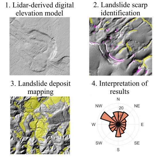
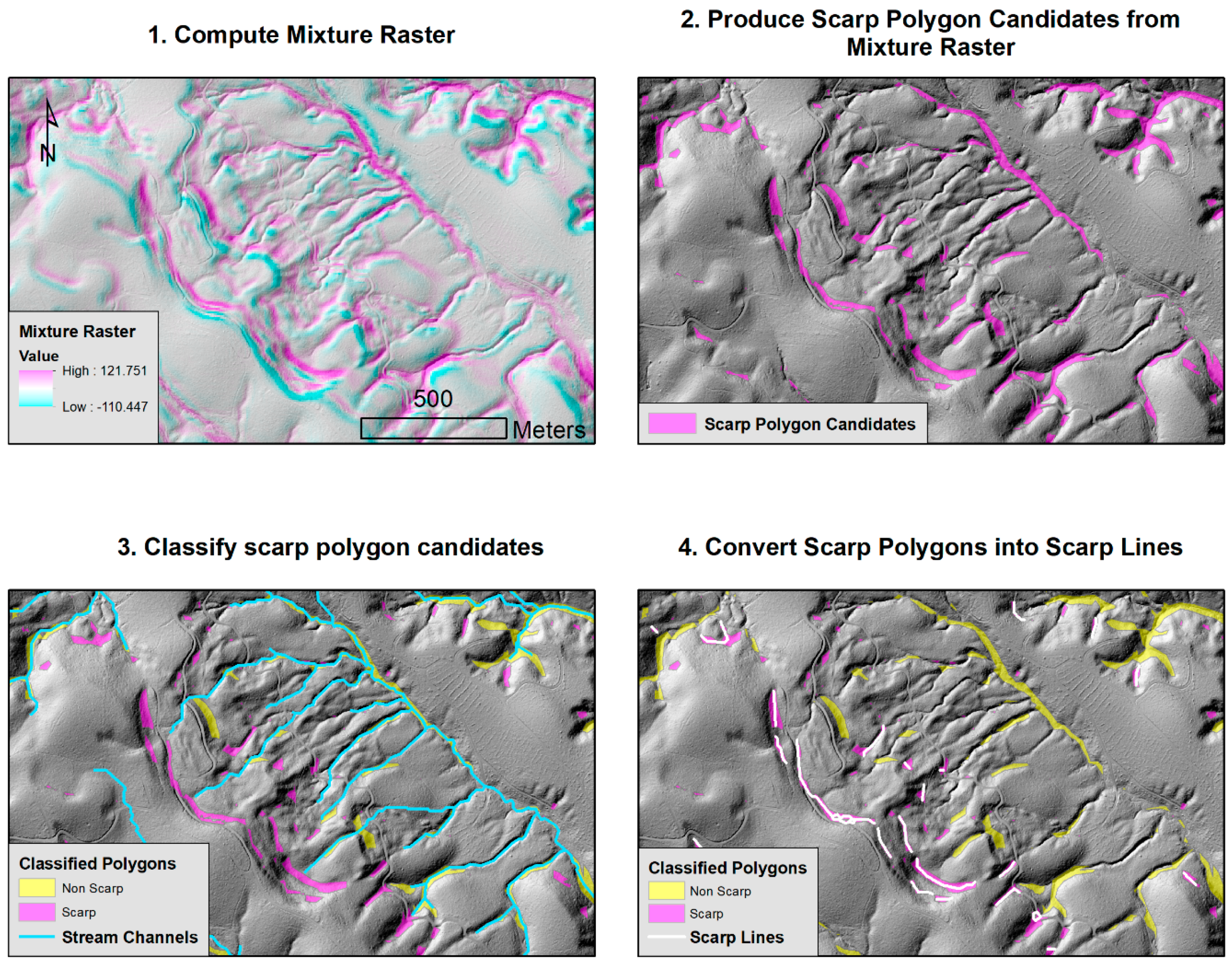
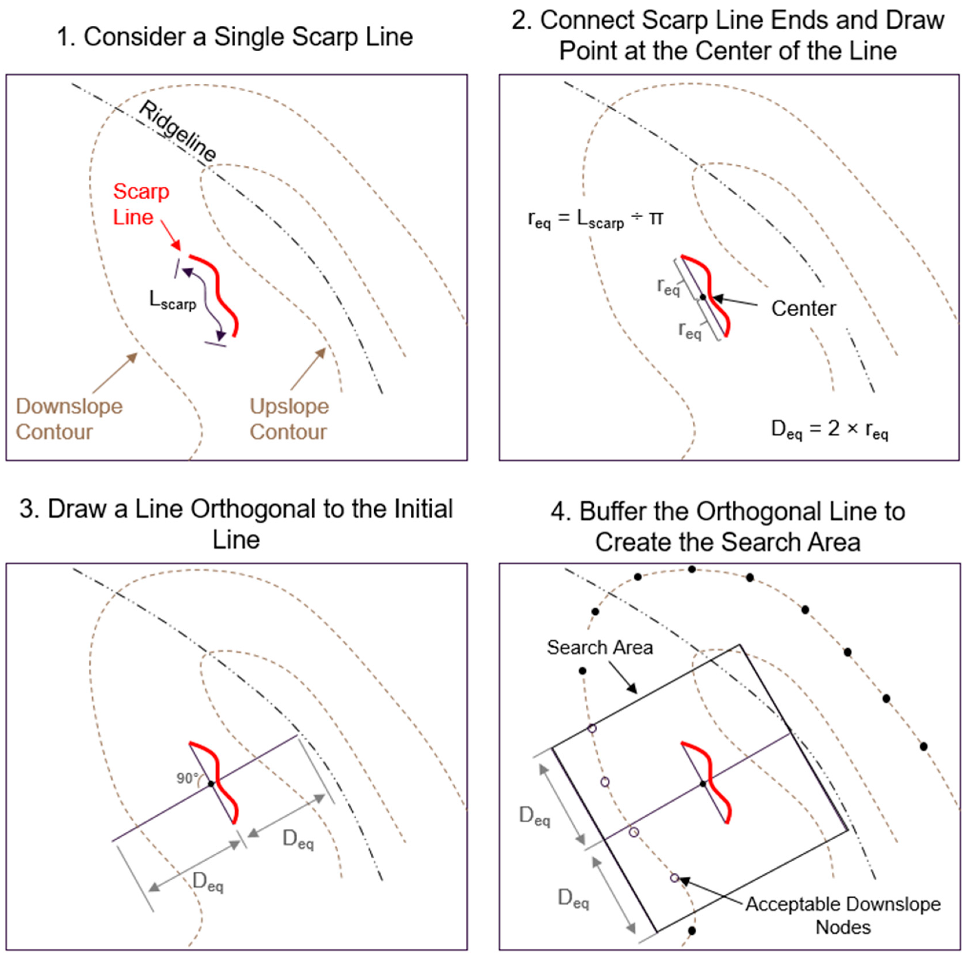
2.1. Scarp Identification and Initial Processing of DEMs

The scarp identification procedure was designed to semi-automatically produce scarp line features that initiate the later process of deposit mapping. Scarps may occur at the head of a landslide, where they are called the main scarp, or throughout the body of a landslide, where they are called minor scarps [31]. Both are considered in the scarp identification process. Scarp lines are polylines typically drawn at the crest of any landslide scarp [19] that represent the uppermost extent of some discrete landslide movement. SICCM has chosen instead to use polylines drawn at the base of the scarp because it helps to reduce over-prediction. Since SICCM relies on scarp identification to initiate deposit identification, more accurately mapping these scarp lines should improve delineation of landslide deposits. SICCM can automatically produce landslide scarp lines and subsequently map landslide deposits in a simple and efficient process, but may not be universally applicable for all mapping purposes and geologic settings. These limitations may, however, be mitigated through human interpretation and intervention at key stages in the aforementioned scarp delineation process. The sensitivity of these interventions is discussed herein.

The following sections describe the key steps in the scarp identification process of SICCM in detail. Prior to identifying the scarps, preliminary processing of LIDAR-derived DEMs reduces artifacts occurring from interpolation in areas of low point density and failed removal of vegetation in obtaining a bare earth model. Afterwards, scarp features are mapped and filtered using several DEM derivatives such as slope and curvature.

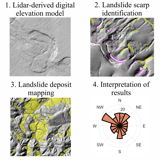
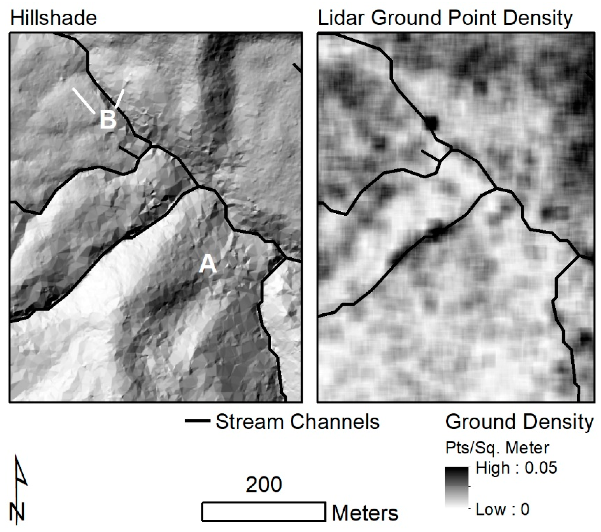
2.1.1. Preliminary Processing of Digital Elevation Models

LIDAR has enhanced mapping of landslide features by providing detailed data that may be processed to remove vegetation to derive accurate ground (bare-earth) surface models and, subsequently, better identify geomorphic features [17]. Thus, SICCM has been designed to map using LIDAR-derived DEMs given LIDAR’s high quality and ability to capture important topographic features. Nonetheless, processing artifacts and data quality should be considered during its application since quality can vary somewhat between different LIDAR DEMs depending on the complexity of the terrain, vegetation, and acquisition procedures. Even within a LIDAR DEM, there remains variability caused by differing LIDAR point density (Figure 1) and amounts of vegetative cover. In the study areas evaluated in this paper located in western Oregon, two common issues were observed with the basic LIDAR datasets: (1) sparse ground points were observed due to the presence of dense forest canopies, and (2) in some cases, there was a failure to completely isolate ground points from vegetation points. These common processing issues both influence the elevation values of resulting DEMs and especially topographic derivatives derived from them. Infrequent ground points meant many DEM cells did not correspond to direct LIDAR measurements and were assigned a value by interpolation, resulting in faceted terrain when linear interpolation was used (Figure 1A). Furthermore, the failure to completely isolate ground points meant that some vegetation points were used when interpolating a surface for the DEM, which produced inaccurate, small lumps on the terrain (Figure 1B).

The aforementioned data limitations during the creation of DEMs can be problematic because they may result in interpolated terrain that does not accurately represent the true ground surface. To overcome this problem, the DEMs were resampled to a larger cell size capable of hiding effects of the facets, lumps, and other potential noise (Figure 2C). The resampling requires that some detail in the initial DEM be sacrificed, but most significant landslide features still exist at a larger scale. Examples of such features include the rough terrain and scarp flanks visible in Figure 2D–F. Previous work has quantitatively documented that landslide features such as hummocky topography and internal scarps tend to have characteristic spatial scales greater than about 10–15 m [24,32], and that non-landslide features such as pit-mound topography caused by tree turnover, or noise in the LIDAR data have shorter characteristic spatial scales [33,34]. As a result, trial-and-error visual assessment in study areas found that resampling the 0.91-m DEMs to 6-m, removed most noise, while also maintaining the appearance of landslide features. This observation is backed up by a quantitative comparison of SICCM results obtained using different cell sizes presented in the discussion section. No manually inventoried landslides, described later, were smaller in area than 60 m², thus this initial processing step was not considered to have significantly influenced the potential for SICCM to sufficiently map landslides in the study area.

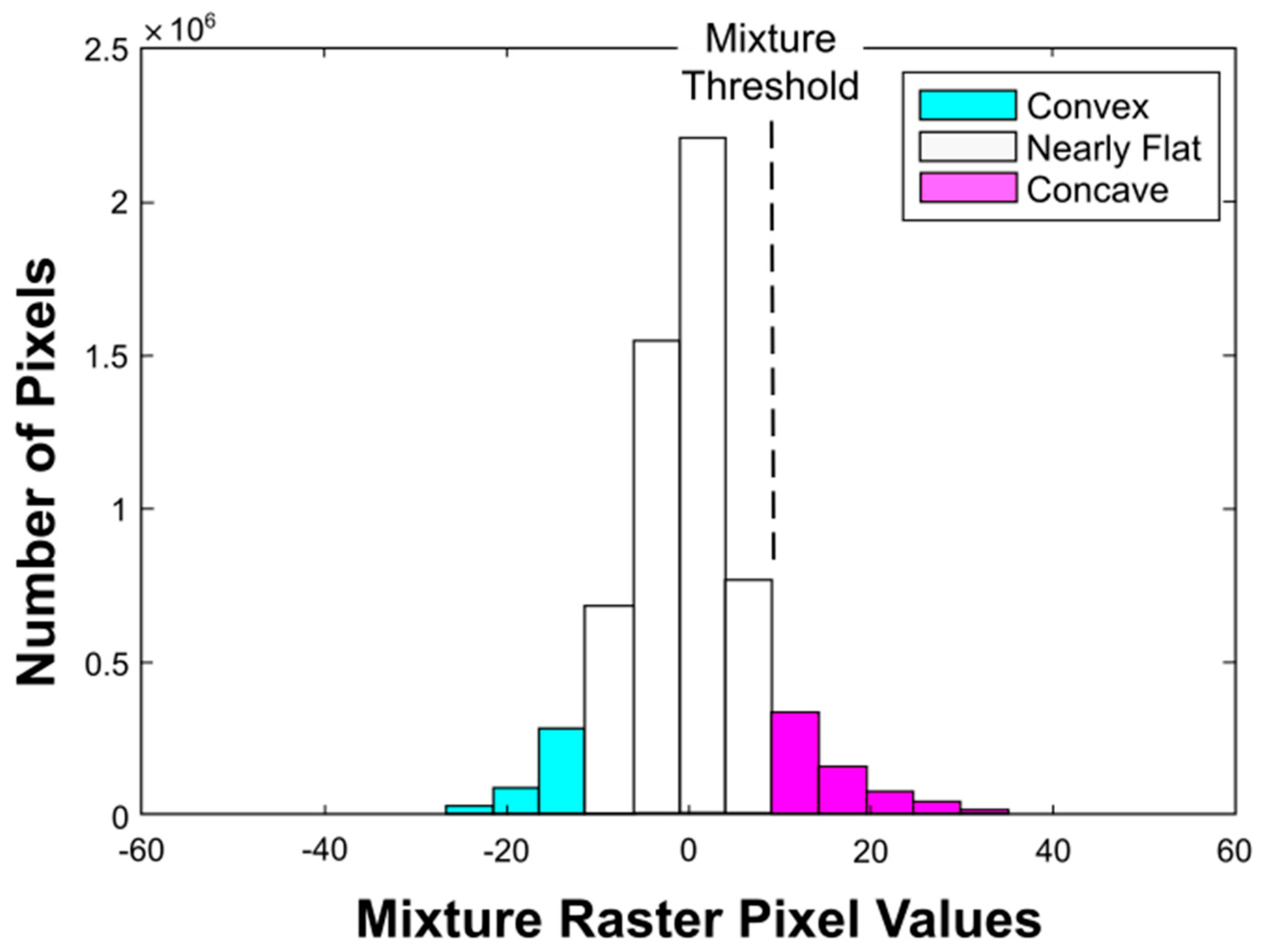
2.1.2. Delineation of Scarp Features

An initial observation of the geomorphic signature of scarp lines manually delineated using the technique presented by [19] was that they correspond with convex profile curvature on relatively steep terrain. At the base of the scarp, slope is also relatively steep, but the terrain has concave profile curvature. To emphasize this signature and enable automated extraction, a DEM derivative computed as the product of slope and profile curvature was produced from the resampled elevation dataset. Slope was computed using the average maximum technique [35] and profile curvature was computed using directional derivatives of slope [36]. This new raster, called the ‘mixture raster’ herein, or the scarp index [37], has large negative values for steep and convex terrain, and large positive values for steep and concave terrain (Figure 3, Step 1). The large positive mixture values, located at the base of scarps and in similar non-scarp terrain, were then extracted to facilitate mapping of scarp terrain. These mixture values were selected because first attempts at extracting pixels with negative mixture values resulted in the extraction of terrain associated with scarps but also of terrain associated with other features, most notably ridgelines. Since ridgelines and main scarps often coincide spatially, separating the two groups objectively proved difficult. The steep and concave terrain included the base of landslide scarps and stream channels. Stream channels could be more easily distinguished from scarps than ridgelines using readily-available stream identification procedures, thus leading to the definition of a new scarp line for SICCM, located at the base of the scarp (Figure 4).

Large positive values of the mixture raster defined an intermediate set of features, called “scarp polygon candidates” (Figure 3, Step 2), which were created to serve as classifiable objects. Direct identification of scarp lines from the mixture raster pixels alone was made difficult by noise, LIDAR artifacts, and false positives associated with stream channels and other gullies. This process mimics the segmentation of object-oriented approaches introduced previously. Scarp polygon candidates comprise terrain surrounding potential scarp lines or other similar topography. These polygons were produced by extracting all mixture pixels with a value greater than a predetermined threshold and then drawing an outline around those pixels. The threshold used to isolate scarp polygon candidates was obtained from the separation between the second and third classes determined by a three-class, Jenks Natural Breaks [38] optimization (Figure 5). This threshold enables adaptation to mixture rasters from different terrain while maintaining reasonable results. However, adjustment of this threshold and interpretation may be performed in order to calibrate delineation of scarp polygon candidates. As illustrated in Figure 5, increasing the threshold results in fewer extracted pixels and smaller scarp polygon candidates. Decreasing the threshold produces the opposite result. For the study areas described later in this study, no alternative threshold appeared to be an improvement over the natural breaks value; nevertheless, other mapping in other terrain may benefit from this manipulation.

Following extraction of scarp polygon candidates, classification was performed based on the spatial correspondence of the polygons with other objects derived from the resampled DEM. The resampled DEM was selected over the initial DEM because it was the same terrain model used to produce the scarp polygon candidates being classified, but it should also be noted that this choice leads to a major reduction in computation time. In this study, intersection with delineated stream channels was deemed an intuitive and effective determination of scarp candidates that were not associated with landslide scarps. Additional geographic information system (GIS) datasets that correspond to possible false positives, such as roads or rock outcroppings could be used to screen those features. Machine learning classifiers would also be suitable for this purpose; however, the simplicity and computational efficiency of isolating non-scarp polygons that spatially correspond to the gullies of stream channels was effective for the proposed study areas. Stream channel polylines were identified following an existing approach [39] with an accumulation threshold of two hectares derived from trial-and-error testing. The selected value gave a balance of polylines of acceptable length. Use of smaller accumulation thresholds provided longer stream channel polylines, which would result in possible removal of scarp polygon candidates that accurately capture main scarp topography. A larger accumulation threshold would yield the opposite, and not all polygons associated with stream channels would be classified. In some settings, expert judgement may aid in the selection of a threshold that is appropriate for the segregation of true and false positives for scarp polygon candidates. When scarp polygon candidates directly intersected stream channel polylines, they were classified as non-scarp polygons (Figure 3, Step 3). The remaining scarp polygon candidates were then classified as scarp polygons and further processed into polyline feature for use in the mapping of landslide deposits.

To provide a set of positively-identified scarp lines compatible with delineation of landslide deposits using CCM, positively identified scarp polygon candidates were isolated and thinned into scarp lines through implementation of the thinning process of Zhan [40], shown in Step 4 of Figure 3. Since the scarp lines needed to correspond with three-dimensional terrain, they were then assigned elevation values along their length at a spacing equal to the cell size of the resampled DEM that they were derived from.

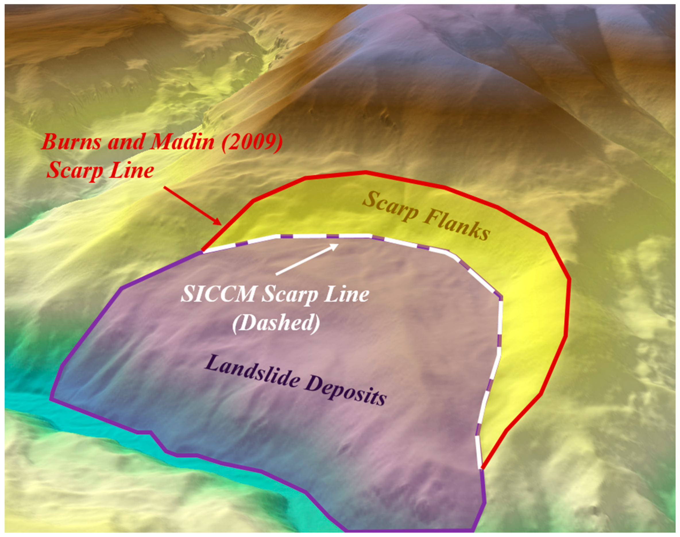
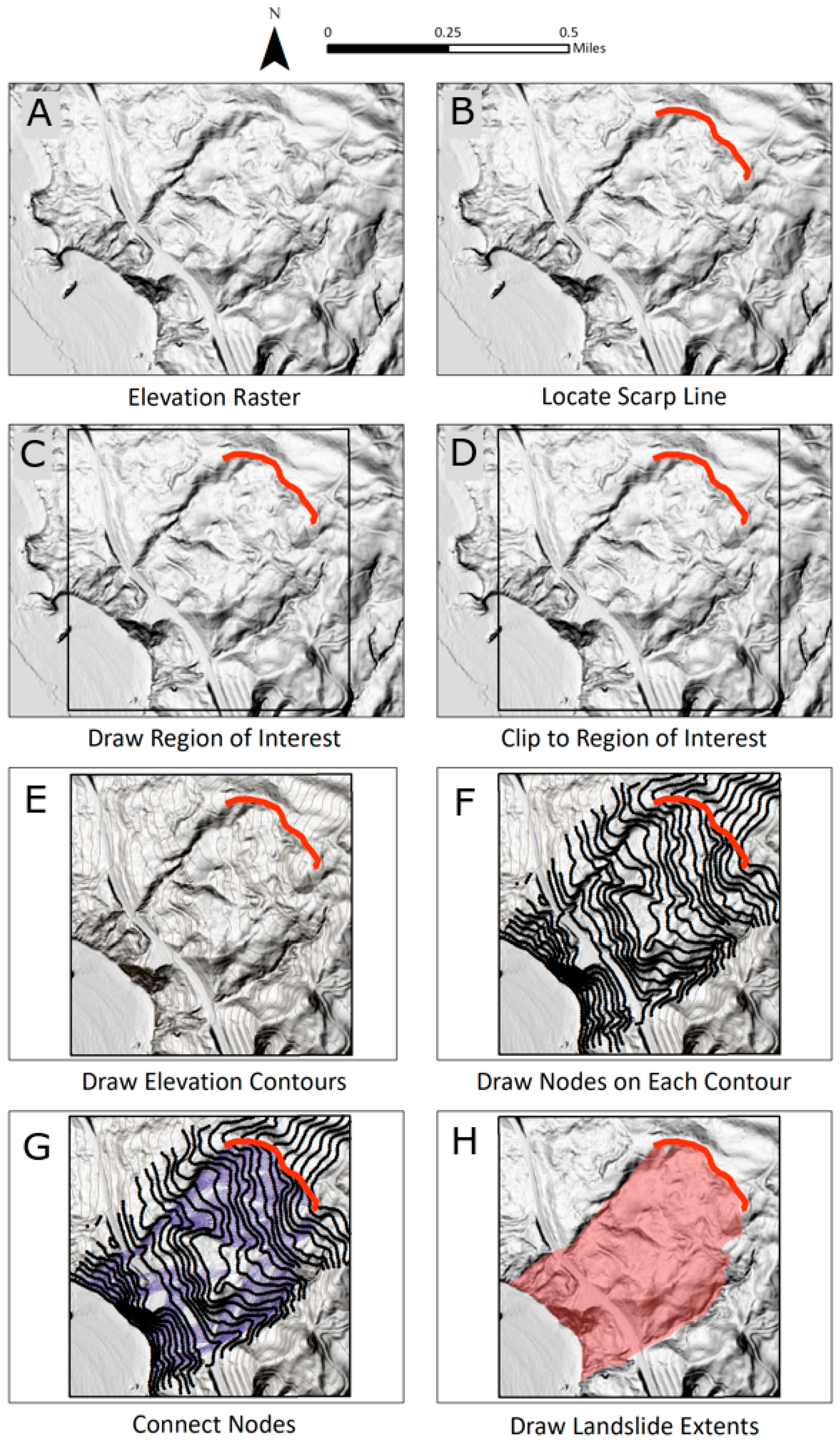
2.2. Deposit Mapping

SICCM uses the scarp polylines to next map deposits below them. The first step in this process is to draw contours on the DEM with the contour interval, ΔE_z., and place nodes along each contour with a node spacing, L_n, as was done by Leshchinsky et al. [30]. In a departure from Leshchinsky et al. [30], the scarp lines are introduced and assigned nodes, also at L_n. Scarp line geometry is then used to define a region of interest around one scarp line at a time, in which the algorithm searches for nodes on the adjacent downslope contour to the scarp line. The search for downslope nodes is limited to within the region of interest to improve computational efficiency. The scarp line nodes are then connected to the downslope nodes within the region of interest, and the slope and number of connections are evaluated. Connections are removed if their slopes fall below the active slope, Δ_active, or if there are more connections than the specified branch parameter, B_n. Once all connections between the scarp line nodes and the nodes on the immediate downslope contour have been evaluated, the region of interest is disregarded, and a similar connection and evaluation process is continued until there are no connections remain to the next downslope contour, a process identical to that of Leshchinsky et al. [30]. The landslide deposits emanating from a given scarp line are then taken as a polygon drawn around the outside of the connection network.

The CCM procedure was restructured to (1) provide increased accuracy in mapping and (2) improved adaptability to new geologic and terrain settings. As previously stated, CCM [30] tended to over map and incorrectly identify landslide deposits as a result of solely using a slope threshold to identify scarps. These inaccuracies are mitigated in SICCM through delineation of scarp lines using the scarp identification process, enabling opportunities for interpretation and semi-automation of landslide mapping consistent with that of the manual mapping procedure. Using the scarp lines derived from the scarp identification procedure as an input, a modified version of CCM was used to map landslide deposits (Figure 6). To make this change, identified scarp lines needed to be consistent with the discretization procedure involving nodes and contours placed by CCM. This fundamental modification in the mapping process was incorporated by placing a series of evenly-spaced nodes were along scarp lines at the pre-specified node spacing, which enabled direct connection to downslope nodes and evaluation of the slope of each connection. Previously, an entire DEM was assigned contours and nodes to discretize possible connection paths of landslide deposits. Using this approach, every possible connection between nodes on neighboring contours was assessed—an inefficient and computationally expensive approach towards mapping. Computational efficiency was enhanced by creating localized DEMs for each landslide feature, done by clipping the resampled DEM (Figure 6A) based on an associated, predetermined scarp line (Figure 6B) to discretize a region of interest (Figure 6C,D). Within this region of interest, elevation contours and nodes were then assigned the localized DEM (Figure 6E,F) for application of the CCM procedure. Finally, using all of the original CCM inputs with the exception of Δ_scarp, connections are made downslope until their slope becomes more gradual than Δ_active, subsequently terminating the lower boundary of the mesh that delineates the landslide deposits (Figure 6G). Thereafter, the extents of landslide deposit may be defined by the polygon outline by the aforementioned mesh (Figure 6H).

Although the separate scarp identification process enables improved accuracy, it also introduced computational challenges associated with connectivity. Specifically, nodes downslope from the scarp line were not always identified correctly. For example, scarps located near ridgelines often identified potential downslope nodes that exist on the opposite face of a ridge. This issue occurs because contours may be a rather coarse representation of the ground surface. This problem was mitigated by defining a search area within the region of interest (Figure 7) to prevent downslope nodes behind the scarp line from being connected to the scarp line’s nodes, thus ensuring the appropriate path for connectivity in the landslide delineation process. The search area dimensions are set by the length of the scarp line, and are based on the assumption that the scarp line has the shape of a semi-circle arc. The diameter and radius, D_eq and r_eq, are back-calculated from the scarp line length, L_scarp, as if it were half the circumference of a circle, and the search area extends a distance 2D_eq in the scarp-normal and scarp-parallel directions. This assumed geometry is not always reflected in the true shape of a scarp line, but was deemed reasonable for simplicity and computational efficiency, facilitating mapping over large areas. Through these fundamental changes, the proposed SICCM procedure presents the opportunity for enhanced accuracy and computational efficiency.

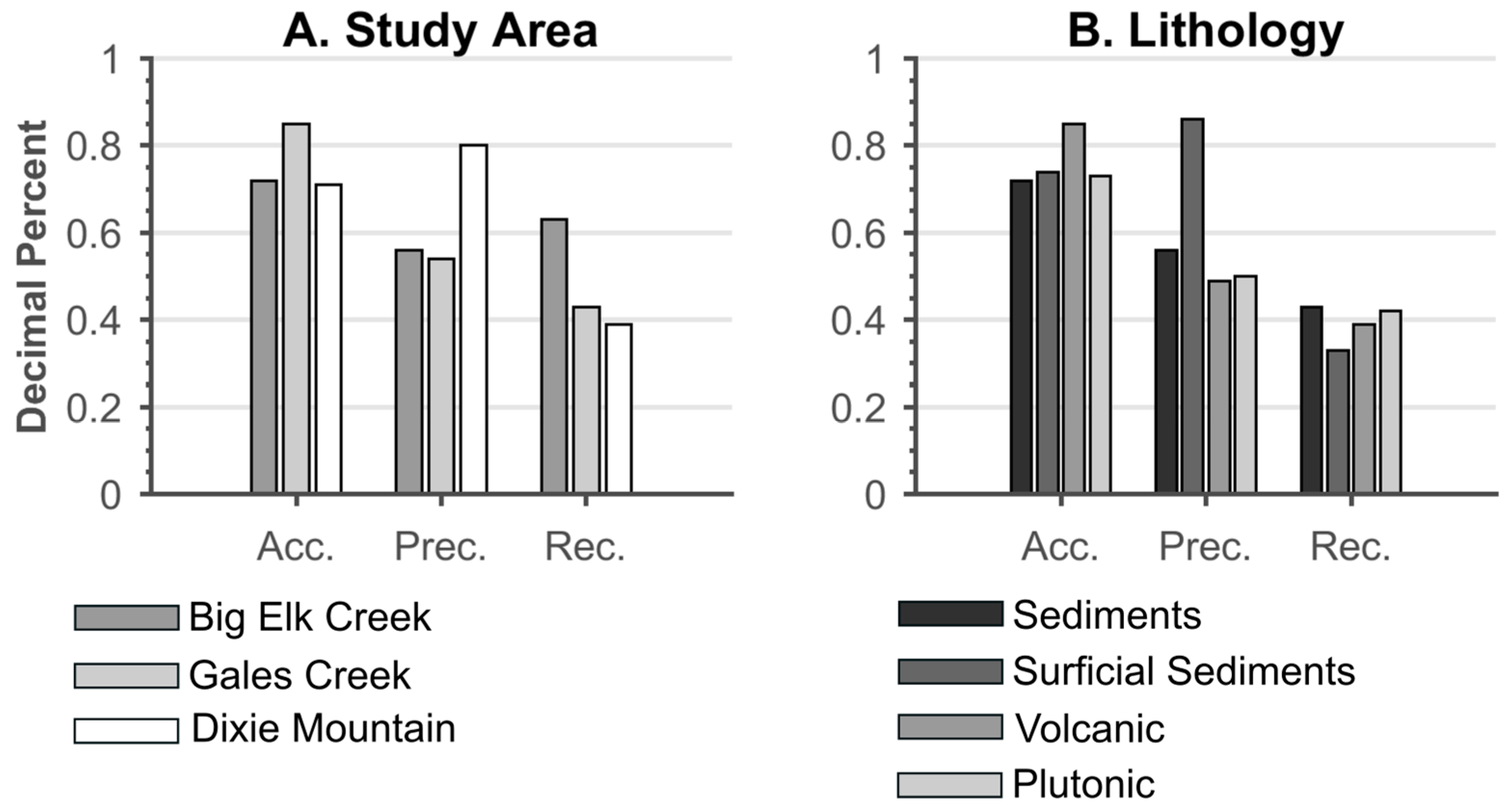
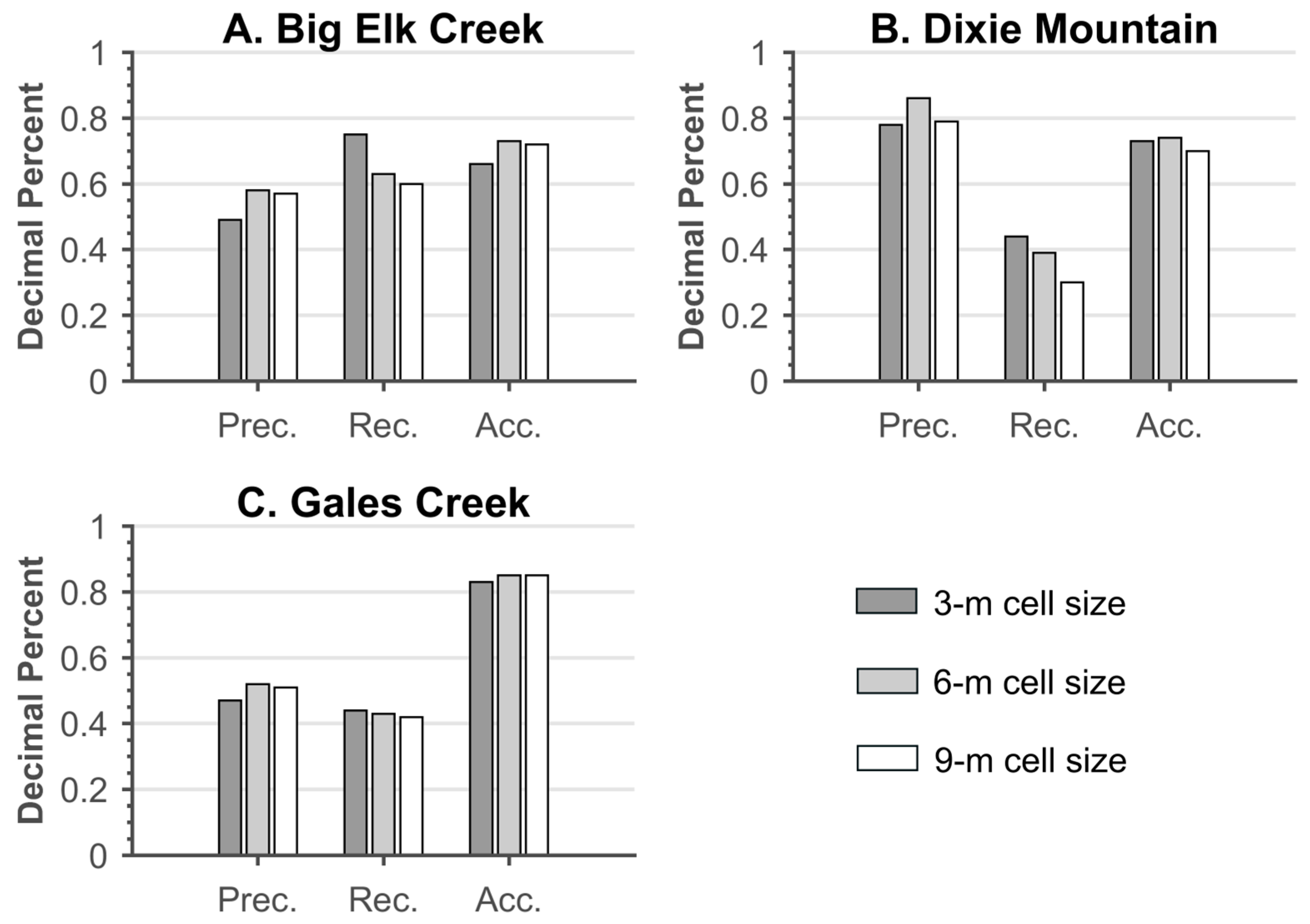
2.3. Assessment of Accuracy

In order to characterize the efficacy of any model, a rigorous assessment of accuracy is required. Assessment of the accuracy of landslide mapping, however, is a challenging endeavor, as the ‘correct’ comparative dataset—a manually mapped landslide inventory—is subjective, created based on the judgment of the individual delineating the landslide deposits [16]. Nonetheless, recent documentation on the landslide mapping process (e.g., [19]) has strived to enhance consistency in the creation of landslide inventories. In this study, the accuracy of SICCM was assessed in comparison to expertly mapped inventories in western Oregon created by the Oregon Department of Geology and Mineral Industries (DOGAMI) that adhere to the standard outlined by Burns and Madin [19]. Each inventory includes scarp lines, scarp flanks, and landslide deposits. Because SICCM maps downslope from the bottom of the scarp flanks, comparisons were only made to the deposits. SICCM and DOGAMI deposits were converted into binary rasters, with a value of 1 for deposits and 0 for everything else, and correspondence was computed pixel by pixel and used to compute a confusion matrix.

There are numerous methods used to assess the predictive performance of a model, although in terms of landslide inventories, they most commonly reduce to measures of over-prediction, under-prediction, and overall accuracy. Three confusion matrix-derived measures that fit into those categories are assessed herein: precision, recall, and accuracy. All three measures range from zero to one, with one representing perfect performance. Precision is defined as

$$\mathrm{Precision}=\frac{\mathrm{SICCM}\mathrm{Deposit}\mathrm{Area}\left(\mathrm{SDA}\right)\cap \mathrm{Expert}\mathrm{Deposit}\mathrm{Area}\left(\mathrm{EDA}\right)}{\mathrm{SICCM}\mathrm{Deposit}\mathrm{Area}\left(\mathrm{SDA}\right)}$$

(1)

where SDA is the SICCM deposit area, EDA is the expert deposit area, and ∩ is the geometric intersection. Precision (Equation (1)) measures how much of retrieved information was pertinent [41]. In this case, pertinence is landslide deposit area correctly identified by SICCM. Areas mapped by SICCM as landslide deposits that do not agree with the expert inventory deposits are considered impertinent. High values of precision would imply low over-prediction but may also mean under-prediction if all SICCM mapped landslides fit within the extents of expert mapped landslides. Recall is defined as

$$\mathrm{Recall}=\frac{\mathrm{SDA}\cap \mathrm{EDA}}{\mathrm{EDA}}$$

(2)

where SDA, EDA, and $\cap$ remain as defined above. Recall (Equation (2)) measures the proportion of all pertinent information that was retrieved. Low values of recall indicate that little relevant information was retrieved, and that under-prediction has occurred. High recall can also result from severe over-prediction. Finally, Accuracy is defined as

$$\mathrm{Accuracy}=\frac{\left(\mathrm{SDA}\cap \mathrm{EDA}\right)\cup \left(\mathrm{SICCM}\mathrm{Non}\mathrm{Deposit}\mathrm{Area}\cap \mathrm{Expert}\mathrm{Non}\mathrm{Deposit}\mathrm{Area}\right)}{\mathrm{Total}\mathrm{Area}\mathrm{Mapped}}$$

(3)

where SDA, EDA, and $\cap$ remain as defined above, and $\cup$ is the geometic union. Unlike precision and recall, accuracy (Equation (3)) considers both pertinent and impertinent information. Perfect (100%) accuracy would indicate that SICCM deposits and expert deposits were mapped in the same locations and nowhere else. While accuracy may appear to be a universal comparison, it can become biased in cases where amounts of pertinent and impertinent information are disproportionate. Consider for example, that 10 percent of the terrain has been mapped as landslide deposits by an expert. If SICCM were to predict none of the terrain as landslide deposits, accuracy would still be 90 percent. Landslide proportions of the study areas presented in this paper range from 16 to 39 percent, meaning that high measures of accuracy would be possible by predicting all terrain as non-landslide.

Using the aforementioned SICCM procedure and the prescribed metrics for model accuracy, recall, and precision, creation of landslide inventories and comparison to expertly-mapped inventories is discussed in the following section.

3. Results

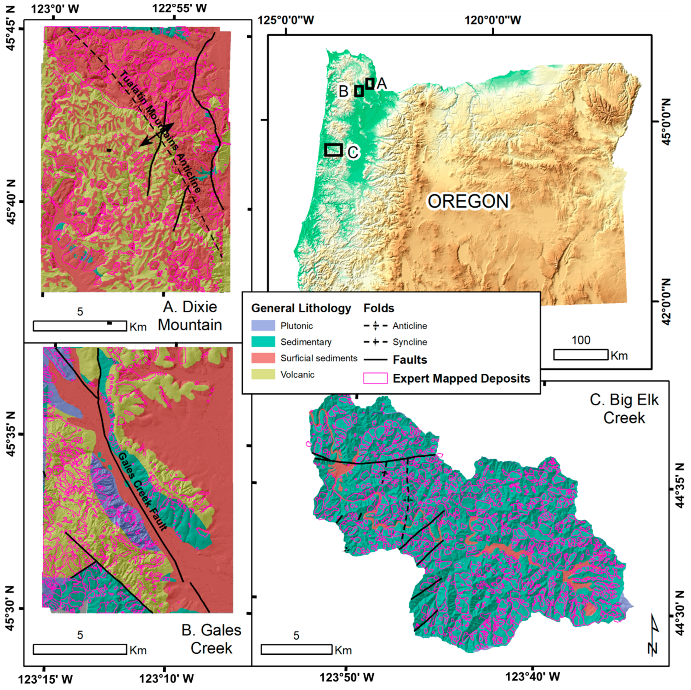
3.1. Study Area Datasets

Three study areas were selected for use in testing the proposed SICCM framework. All of which have existing landslide inventories prepared by expert interpretation of LIDAR-derived imagery that may be used for comparison. The selected regions are all in western Oregon, USA, but they represent diverse geomorphic and geologic conditions, enabling an opportunity to test SICCM’s changes in terrain. The specific study areas include the Dixie Mountain and Gales Creek USGS 7.5 min quadrangles, as well as the Big Elk Creek watershed. Site conditions for each of these areas are summarized in Figure 8 and

Table 1. General characteristics of each study area.

	Dixie Mountain Quadrangle	Gales Creek Quadrangle	Big Elk Creek Watershed
DEM cell size	0.91 m	0.91 m	0.91 m
Size of area mapped	143 km2	144 km2	230 km2
Percent of area mapped as landslide deposits in existing inventory	39%	16%	33%
Number of deposit features mapped	739	698	1189
Mean slope (6.1-m DEM)	15.4°	11.1°	25.1°
Standard deviation of slope (6.1-m DEM)	10.6°	10.5°	12.3°
Elevation range	~0 m to 540 m	50 m to 550 m	~0 m to 1030 m
Date of LIDAR acquisition	3/15/07–5/09/07		9/02/11–11/22/11
Reference for LIDAR data	[42]		[43]
Reference for existing inventory	[44]	[45]	[2]

, and additional detail is provided in the following sections.

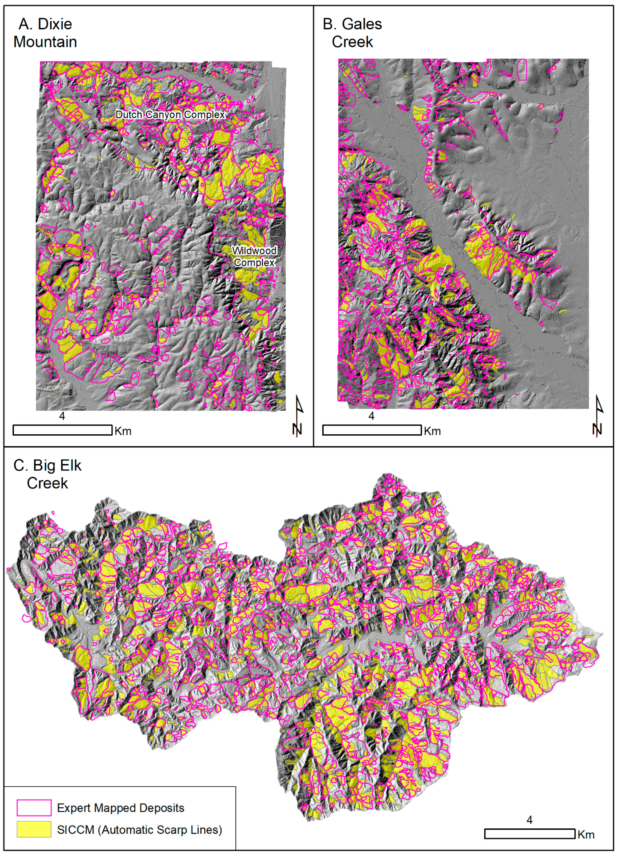
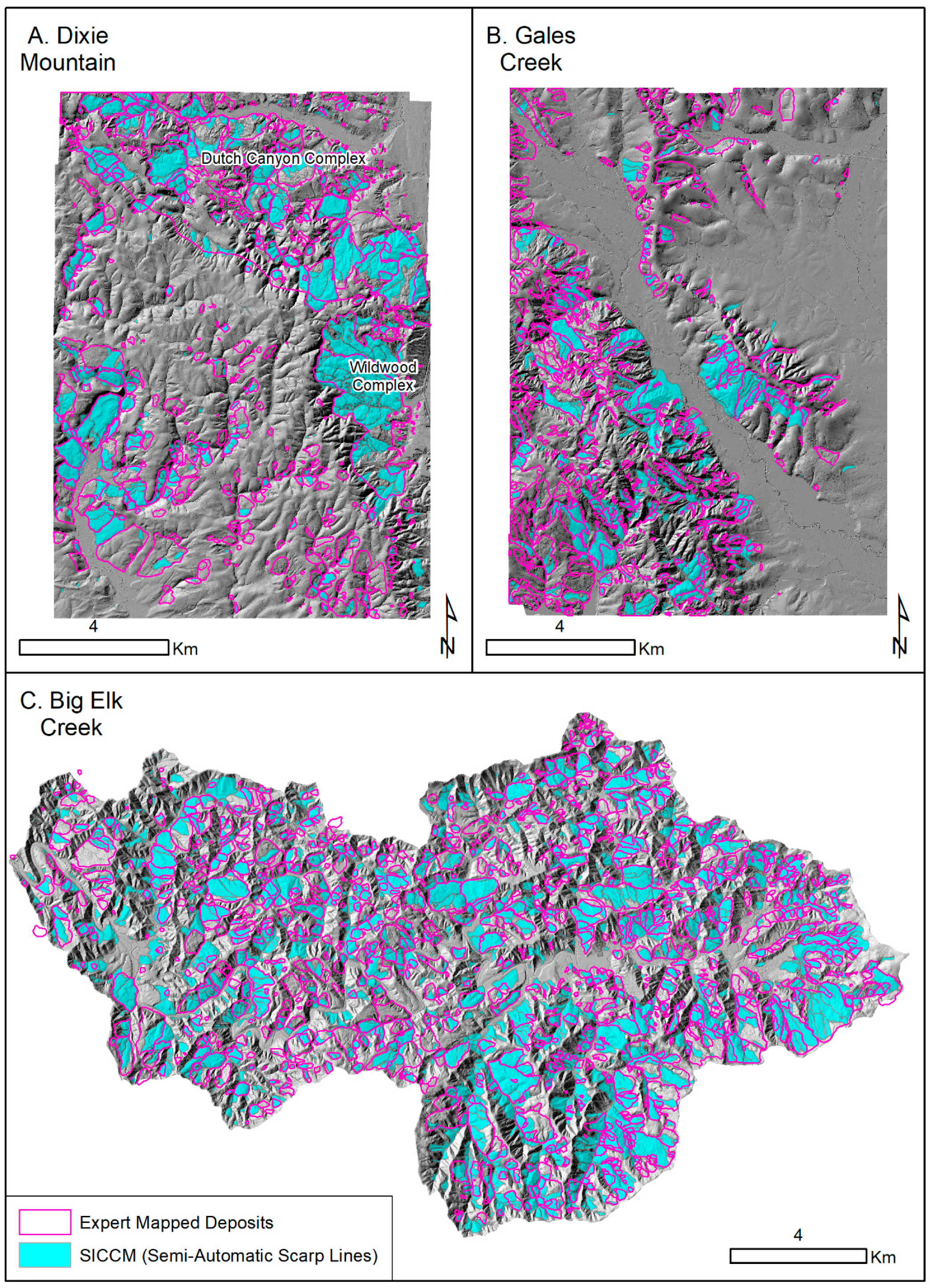
3.1.1. Dixie Mountain Quadrangle

The Dixie Mountain quadrangle is located within the Tualatin Mountains of northwestern Oregon. The geology within the quadrangle is split into southwest and northeast groups by the Tualatin Mountains Anticline [46]. Southwest of the anticline, surficial loess deposits include many small, shallow landslides, and northeast of the anticline, weak marine sandstone sediments of the Scappoose Formation form two major landslide complexes. Additionally, the northeast corner, as well as much of the deposits from the two complexes, are intersected by the Portland Hills Fault Zone. Most of the area, except for several small clear-cuts, is covered by dense vegetation. Overall, 739 landslide features were mapped by geologists using LIDAR (0.91 m resolution) in this region. These landslides were classified into 0% translational landslides, 4% rotational landslides, 27% debris flows and earthflows, and 69% landslide complexes. Deposit sizes range from 74 square meters to 29 million square meters. Notably, over 39% of the region has been mapped as landslide deposits, mainly owing to the broad region in the northeast that includes several landslide complexes.

3.1.2. Gales Creek Quadrangle

The Gales Creek quadrangle is located approximately 20 km southwest of the Dixie Mountain quadrangle in the Northern Oregon Coast Range. Despite its proximity to Dixie Mountain, the Gales Creek quadrangle exhibits very different geology and landslide activity. The most recent geologic map [47] indicates that the quadrangle is split into southwest and northeast portions by the Gales Creek Fault. Southwest of the fault, inventoried landslides are prevalent and appear to occur evenly throughout the terrain. Northeast of the fault, and near the center of the quadrangle, landslides mainly occur on the southwest face of a major ridge. The ridge is comprised of mainly interbedded Pittsburg Bluff Formation sandstone and mudstone sediments, but landslide activity does not tend to occur on its northeast slopes where Columbia River Basalts overlie the sediments. Overall, 698 landslide features were mapped by geologists using LIDAR (0.91 m resolution) in this region. These landslide features were classified into 0% translational landslides, 5% rotational landslides, 13% debris flows and earthflows, and 82% landslide complexes. Over 16% of the region has been mapped as a landslide deposit, consisting of features of varying sizes, ranging from 62 m² to 1.3 million m².

3.1.3. Big Elk Creek Watershed

The Big Elk Creek Watershed is located within in the Central Oregon Coast Range, approximately 10 km east of Newport, Oregon. The site was selected, in part, because its geology differed significantly from the other two sites. The watershed is located within the interbedded sandstone and siltstone Tyee Formation, which is notorious for high landslide activity [2]. Geologic units in the Big Elk Creek Watershed have not been mapped during the last 50 years, but recent geologic mapping has been performed adjacent to the watershed [48]. Landslide activity in the Tyee formation primarily tends to occur along dipping sandstone bedding planes [2,48]. Overall, 1188 landslide features were mapped by geologists using LIDAR (0.91 m resolution) in this region, classified into 15% translational landslides, 13% rotational landslides, 3% debris flows and earthflows, and 69% landslide complexes. 33% of the region has been mapped as landslide deposits, ranging from 91 square meters to 17 million square meters, resulting from the large earthflows concentrated in the southeast portion of this region.

3.2. Application of SICCM

The SICCM procedure was performed for each study area using scarp lines generated automatically (no adjustment of mixture threshold or reassignment of class) and semi-automatically (reassignment of class). Identical CCM deposit mapping parameters were used for each set of scarps lines. These parameters (B_n = 5, Δ_active = 2°, L_n = 6 m, ΔE_z = 6 m), were selected through a sensitivity analysis performed on the Big Elk Creek study area. The sensitivity analysis and the influence of these parameters on results are described in the discussion. While the CCM input parameters may affect the accuracy, precision and recall of the results compared to expertly-mapped inventories, the results were not exceptionally sensitive to inputs, with the exception of branch parameter, B_n. This insensitivity results from the consistent use of predefined scarps from which deposits are mapped. Parameter choices and time spent for each trial are presented in

Table 2. Numerical summary of scarp identification results. Landslide areas apply only to deposits produced from automatic scarp lines.

	Dixie Mountain Quadrangle	Gales Creek Quadrangle	Big Elk Creek Watershed
Mapping cell size	6.1 m	6.1 m	6.1 m
Mixture threshold	4.29 deg-m	4.02 deg-m	6.02 deg-m
Accumulation area used to define stream channels	2 ha	2 ha	2 ha
Time spent on automated processes for scarp lines	6 min	6 min	12 min
Time spent reassigning polygons for semi-automatic scarp lines	6 min	4 min	10 min
Branch parameter, Bn	5	5	5
Active slope, Δactive	2 deg	2 deg	2 deg
Node spacing, Ln	6 m	6 m	6 m
Contour interval, ΔEz	6 m	6 m	6 m
Time spent on automated processes for deposit mapping (semi-automatic)	45 min (47 min)	40 min (45 min)	204 min (223 min)
Number of deposit features (semi-automatic)	1144 (1267)	792 (910)	2644 (2758)
Area mapped as landslide deposits (semi-automatic)	41 km2 (51 km2)	30 km2 (33 km2)	145 km2 (156 km2)
Minimum landslide area	58 m2	68 m2	28 m2
Mean landslide area	36,077 m2	37,589 m2	54,748 m2
Maximum landslide area	1,096,829 m2	1,059,723 m2	1,010,183 m2

. Automated tasks were performed on an Intel Xeon E5620 processor running at 2.40 GHz with 24 GB of RAM.

Table 2 shows two major differences between SICCM deposits mapped with automatic scarp lines and the expert mapped deposits. First, although the reported SICCM deposit areas are comparable to areas reported previously for the expert mapped deposits, the primary difference is that the largest SICCM deposits for Big Elk Creek and Dixie Mountain are an order or magnitude smaller than the largest expert mapped deposits. Second, the number of deposit features mapped by SICCM, from either automatic or semi-automatic scarp lines, is generally much larger than the number of expert mapped deposit features (Table 1). For reference, the number of expert mapped deposits was 739 at Dixie Mountain; 698 at Gales Creek; and 1189 at Big Elk Creek.

Landslide deposit inventories produced using SICCM automatic and semi-automatic scarp lines are mapped in Figure 9 and Figure 10, respectively. The map also displays the expert mapped deposits for the Dixie Mountain [44] and Gales Creek [45] quadrangles, and for the Big Elk Creek Watershed [2] for comparison.

Figure 9 and Figure 10 illustrate the spatial distribution of the SICCM deposits mapped using automatic and semi-automatic scarp lines. Semi-automatic scarp lines failed to produce a visible difference in most of the area mapped, with the only main exception being the Wildwood Complex. Instead, the differences tend to be uniformly distributed across most terrain. To provide an alternative perspective, a quantitative comparison of SICCM deposits with expert mapped deposits is presented in

Table 3. SICCM validation results comparing the effect of semi-automatic and automatic scarp lines. The confusion matrix used to compute accuracy, precision, and recall has been presented in with the fields true positive (TP), false positive (FP), true negative (TN), and false negative (FN). True relates to the landslide inventory and positive refers to the presence of an inventoried landslide.

Study Area	Scarp Lines	TP	FP	TN	FN	Accuracy	Precision	Recall
Dixie Mountain	Automatic	0.15	0.03	0.59	0.24	0.74	0.86	0.39
	Semi-Automatic	0.21	0.05	0.56	0.18	0.77	0.80	0.54
Gales Creek	Automatic	0.07	0.06	0.78	0.09	0.85	0.52	0.43
	Semi-Automatic	0.07	0.06	0.78	0.09	0.85	0.52	0.44
Big Elk Creek	Automatic	0.21	0.15	0.52	0.12	0.73	0.58	0.63
	Semi-Automatic	0.21	0.15	0.52	0.12	0.73	0.59	0.65

. The contents of each confusion matrix used to compute accuracy, precision, and recall have been presented for added transparency of results.

Results presented in Table 3 are characterized by good accuracy, variable precision, and low recall. While accuracy varies only slightly from site to site, precision and recall appear to be inversely related, leaving no clear indication that SICCM mapped one study area better than another. Instead SICCM mapped study areas differently, either under-mapping or over-mapping deposits. The table also reveals that, for the areas studied herein, only marginal gains came from using semi-automatic versus automatic scarp lines.

As mentioned previously, the study areas were selected, in part, because of their diversity in geology. To assess potential trends related to geography and geology, the automatic scarp line accuracy assessment has been divided based on location (Figure 11A) and generalized lithology (Figure 11B). Generalized lithology was chosen from the multitude of available mapped geologic layers because it allowed all three study areas to be compared. Other layers, such as terrane or formation might better relate to landslide activity, but those are not common to all study areas.

Semi-automatic results are left out of Figure 11 because they are only slightly different from the automatic results. The only noticeable improvement to results caused by semi-automatic scarp lines is that of recall at Dixie Mountain. Results displayed by lithology (Figure 11B) only appear to vary for precision and recall in surficial sediments, which were the primary unstable unit at Dixie Mountain. This observation aligns with the values of precision and recall for Dixie Mountain in Figure 11A.

4. Discussion

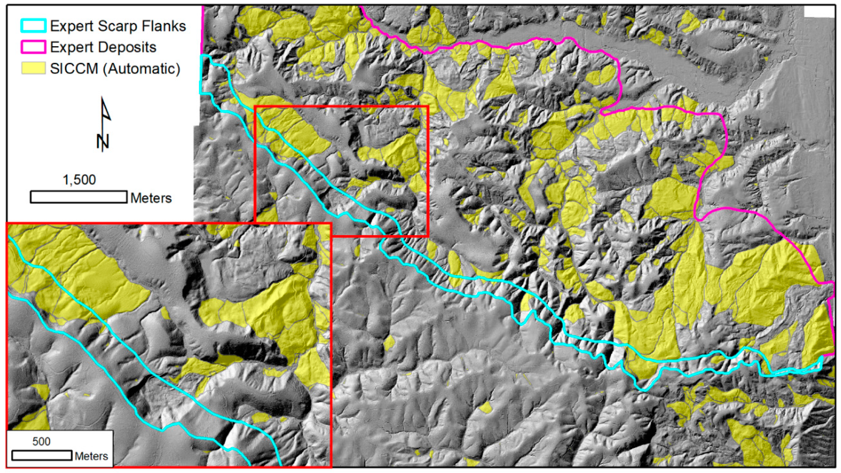
4.1. Quality of SICCM results

The purpose of SICCM’s development was to produce a semi-automated landslide inventory mapping procedure that was capable of rapidly performing basic duties of an expertly mapped inventory. While quantitative measures are important, and will be discussed later in this section, it is important to first qualitatively consider the appearance of SICCM outputs. Figure 12 shows example results produced by SICCM using semi-automatic scarp lines for the Big Elk Creek watershed and the Dixie Mountain quadrangle. As was discussed previously, landslides in the Big Elk Creek area tend to occur on dipping beds of the Tyee Formation. The observation that most landslides occur on northwest slope aspects indicates that the local bedding dips to the northwest (Figure 12A). This observation is inspired by similar interpretation by Burns et al. [2], elsewhere in the Tyee Formation performed using their manually mapped deposits, to illustrate the utility of SICCM outputs. In addition to hinting at geologic structure, the placement of SICCM polygons within the expert mapped deposits also indicates that SICCM is capable of producing natural shapes in reasonable locations. Figure 12B shows the Wildwood Landslide Complex in the Dixie Mountain quadrangle, and illustrates the flexibility in size and shape of landslides that SICCM is capable of mapping. As was the case before, SICCM produced shapes that generally align with those of the expert mapper. A closer look also reveals the numerous smaller polygons within the complex, which originate from the many minor scarps. Comparing this behavior to Figure 12A, with very few small polygons, it is apparent that SICCM has effectively mapped landslides with different levels of activity.

The choice of SICCM results from semi-automatic scarps lines in Figure 12 was made because SICCM mapping of the Wildwood Landslide Complex was significantly improved by the manual reassignment of non-scarp polygons to scarp polygons. Figure 9A shows that much less of the Wildwood Landslide Complex was mapped using automatic scarp lines. The reason behind this change was that scarp polygon candidates had been created in the correct locations but had been classified as non-scarps due to their intersection with stream channel polylines. The landslide complexes at Dixie Mountain were unique among the three study areas because of their large scale and visible signs of weathering. Many of the scarp flanks were gullied, which allowed for stream channels to be mapped across them as well as the scarp polygon candidates. Interventions afforded by SICCM enabled the misclassification to be quickly corrected and explains why the only significant improvement from semi-automatic scarp lines was to recall in Dixie Mountain. Similar scenarios did not exist for the other study areas, as partially expressed by Figure 12A being only mildly different than the corresponding area in Figure 9C. This behavior illustrates that taking the small amount of time to produce semi-automatic scarp lines, despite only showing small improvements in Table 3, is still ordinarily justified to increase landslide mapping quality in some situations.

Elsewhere in the Dixie Mountain quadrangle, there are still discrepancies between SICCM and the expertly mapped deposits, regardless of whether or not semi-automatic scarp lines were produced. The Dutch Canyon Complex, located northwest of the Wildwood Landslide Complex, was only partially mapped by either set of scarp lines. This insufficient mapping is a result of extensive weathering and smoothing of older landslide deposit surfaces by loess deposition, the much larger scale of the landslide complex, and the divergence of expert and SICCM perspectives on mapping. Figure 13 provides a focus on the Dutch Canyon Complex, as expertly mapped, with automatic scarp line SICCM deposits. Note that numerous expertly mapped landslides exist in and around the polygons in the figure, but were omitted for clarity (all expertly mapped deposits may be observed in Figure 9A). Unlike previous figures, expert-mapped scarp flanks are shown. SICCM would have initiated deposits approximately at the bottom of the scarp flanks, had it been able to map scarp lines, but did not because the curvature of this old, large scarp has a much longer wavelength than the 6 m DEM resolution. The inset of Figure 13 displays deposits both mapped and, to the experienced viewer, missed by SICCM, and also the size and number of gullies present on and around the complex’s scarp flanks. More signs of weathering and smooth, potentially stable areas, are shown within the expert deposits in the rest of the figure. All of these features combine to mask the geomorphology needed to map scarp polygon candidates with SICCM. Since SICCM did not map scarp polygon candidates, and ultimately deposits, throughout the complex, recall remains low and true positives are less than false negatives, but this does not indicate that SICCM poorly mapped the area. The numerous small slides mapped by SICCM indicate that the area is very active, and the deposits that were mapped are likely the most recent due to their defined appearance. Additionally, the presence of large expert mapped landslides means that SICCM has more land area for SICCM to map deposits and still be correct, which explains why precision is higher at Dixie Mountain.

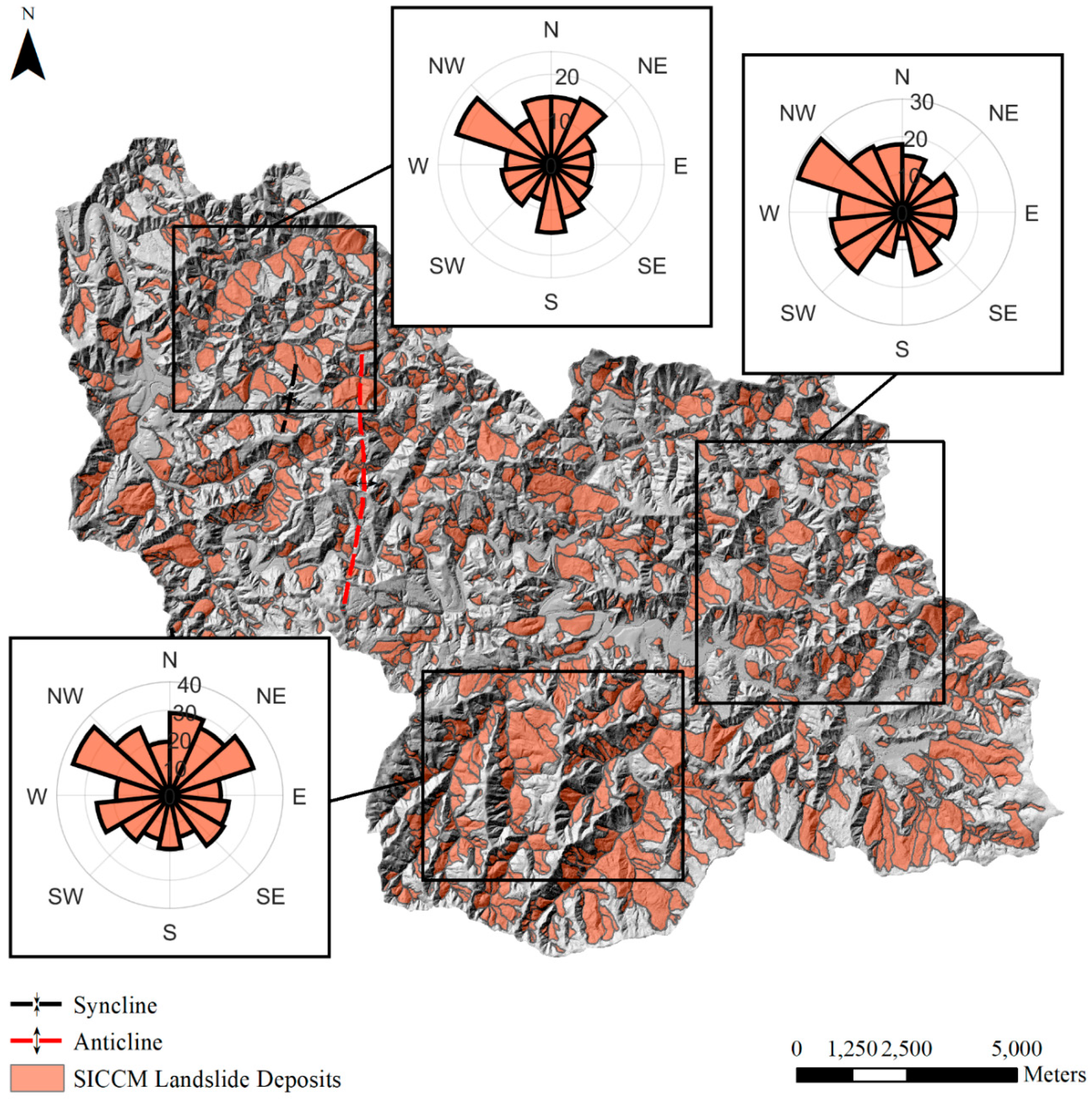
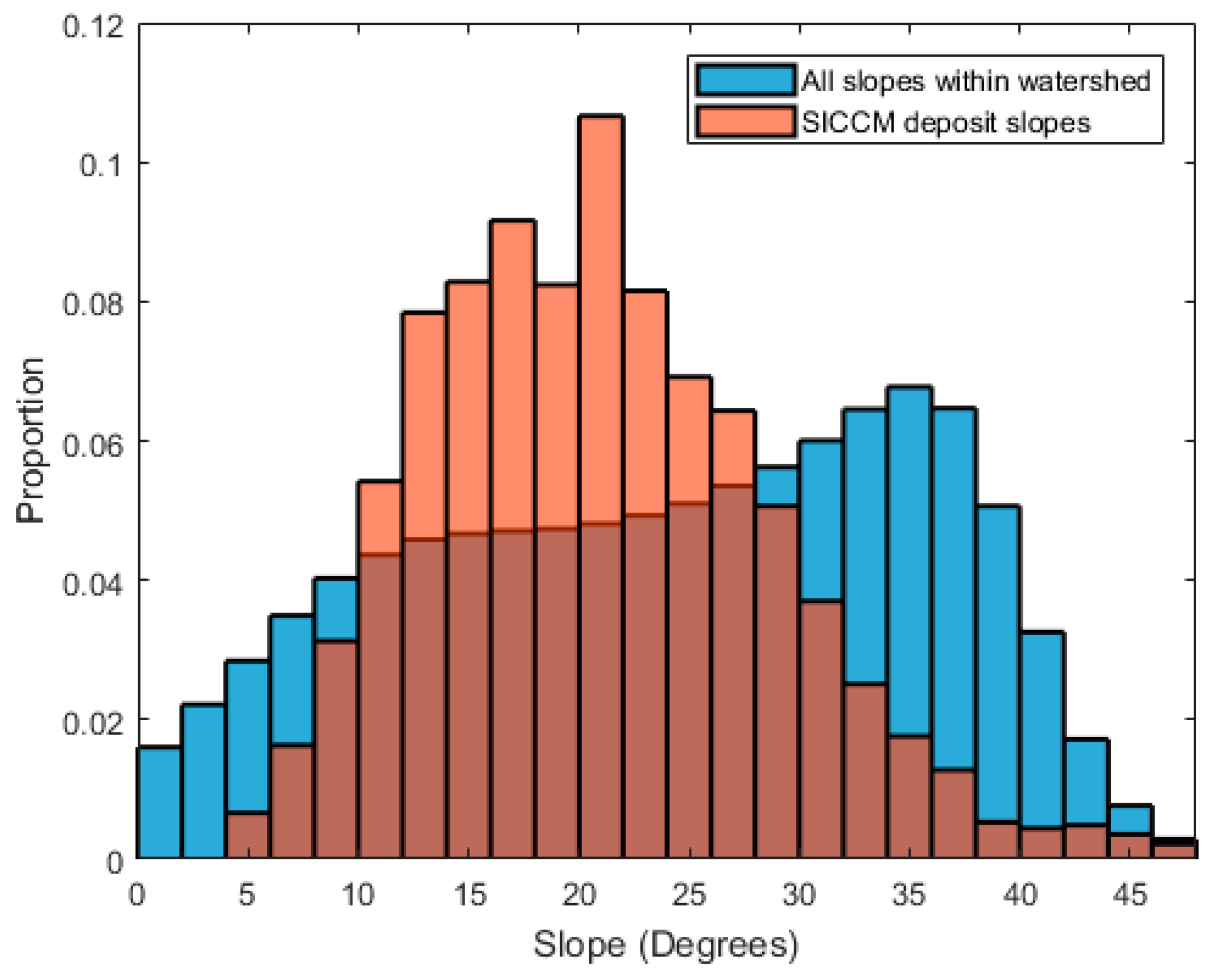
4.2. Quantitative Analyses using SICCM Outputs

The tendency for slope failures to occur in the northwest direction in the Tyee Formation in the Big Elk Creek watershed (Figure 12A) provides a glimpse into the information that may be gained from a detailed landslide inventory produced by SICCM. Analyses of the average surface dip direction of landslide deposits (Figure 14) show that similar trends exist throughout the Big Elk Creek watershed. The plots in Figure 14 were produced using the mean aspect of each SICCM deposit. Plots to the north and east of Figure 14 best illustrate the northwest trend but also show the aspect of deposits facing in other directions. Many of these non-northwest trending deposits have been accurately mapped, but it is also likely than some of them have been erroneously mapped. The south rose plot shows a different trend, with a larger number of deposits also facing the northeast. This change is likely due to a change in direction that bedding dips or in the mechanisms that drive landslides in that area, which may be visible with the presence of large, deep canyons.

In addition to aspect, another useful topographic variable is ground slope. Information regarding landslide susceptibility may be gained by comparing the slopes of landslide deposits to the slopes of adjacent terrain. Figure 15 presents a histogram where the mean deposit slopes are compared to a histogram of all pixels from a 6.1-m slope raster of the watershed. The results show that deposits have a lower gradient than much of the surrounding terrain. Since deposits represent failed terrain, and are not always expected to be steep owing to the dominance of geologic structure, these results are not surprising. However, this figure demonstrates that SICCM-based inventories are valuable as it offers a glimpse at a possible dip angle of the Tyee Formation. This dip trend is reasonable in the context of previous work, which describes dip angles rarely exceeding 15 to 20 degrees in the Tyee Formation, with the likelihood of landslide occurrence increasing significantly with increases in dip.

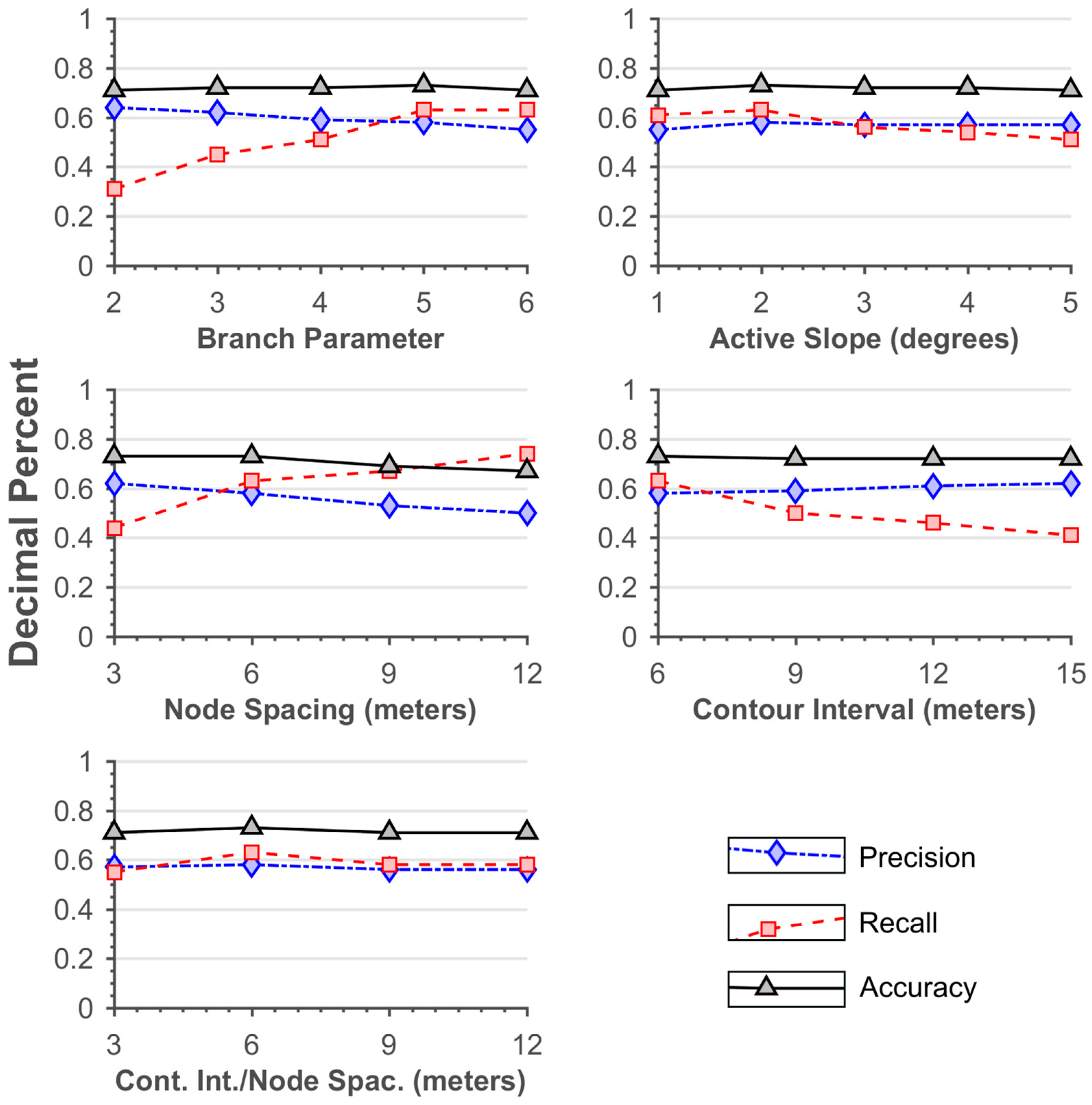
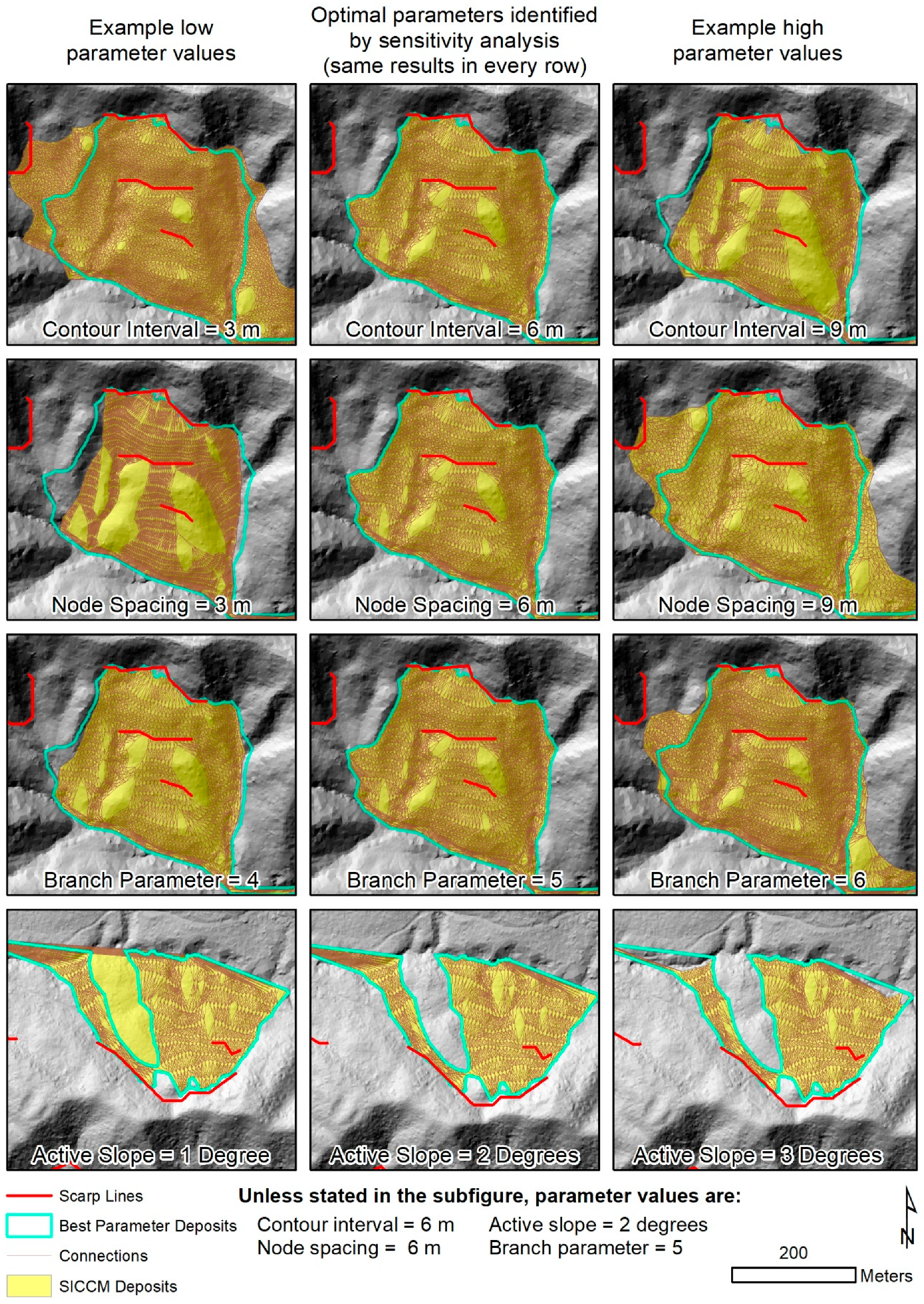
4.3. Sensitivity of Landslide Inventory Maps to SICCM Inputs

During the description of preliminary DEM processing, it was stated that trial-and-error was used to select the cell size for scarp identification. To evaluate the effect of this decision, SICCM results with automatic scarp lines were produced using three-meter and nine-meter cell sizes to supplement the six-meter cell size results. All other settings remained the same, and deposits were mapped from the scarp lines for each resolution. An accuracy assessment produced from these results is presented in Figure 16.

Figure 16 illustrates that the scarp identification cell size does not systematically influence the accuracy assessment measure. On the other hand, behavior of note is the increased recall and decreased precision for the three-meter cell size. The increased recall is desirable in itself, but it is problematic in that is paired with decreased precision that would reduce confidence in analyses like those performed in the previous discussion. Confirmation is given that the six-meter cell size is likely a better option than a three-meter or nine-meter cell size.

An interesting note related to Figure 12, and the different landslide shapes and sizes, is that the input values used to dictate deposit geometry were identical, despite changes in the geologic setting and style of landslide. Values were the same for all three study areas (B_n = 5, Δ_active = 2°, L_n = 6 m, ΔE_z = 6 m), and they were chosen based on the results of a sensitivity analysis (Figure 17). The sensitivity analysis was performed for the Big Elk Creek watershed with a range of parameters observed to be both reasonable and slightly extreme during initial tests. Our goal was to capture the changes in precision, recall, and accuracy for each possible input. Each parameter was varied individually while the other parameters remained stationary, with the exception of L_n (node spacing) and ΔE_z (contour interval), which were also varied together.

Results of the sensitivity analysis indicated that no single set of parameters resulted in the highest precision, recall, and accuracy, and the set that was ultimately selected was chosen qualitatively based on the combination of relatively high values of precision, recall, and accuracy, and the visual appearance of deposit shapes. The appearance of deposit shapes was evaluated by the smoothness of their outline and their correspondence with landslides that were visually apparent in the terrain. A quantitative decision was not possible due to the difficulty in deciding how to best combine precision, recall, and accuracy, when the relative weight of each measure is not known. Aside from helping to select proper inputs, Figure 17 is important because it shows that model performance, in terms of accuracy and precision, is relatively independent of input values. This behavior is generally ideal because it indicates a small cost in the accuracy of landslide mapping, when reasonable SICCM input values are used. SICCM requires few parameters to dictate the geometry of mapped deposits, but reasonable values are easy to select.

Once SICCM has been performed with reasonable values, the values can be further optimized by observing outputs and making minor changes to the inputs. This optimization is possible because the inputs are visually apparent in outputs (Figure 18). Variation in the deposit shape alongside the change in inputs illustrates that, despite the insensitivity of the method to input values, their optimization is useful for producing deposits with smooth, less angular outlines that appear more like an expert inventory.

Figure 18 shows that optimization of SICCM output shapes is a simple process. Decreases to ΔE_z cause the deposit shape to widen, while decreases to L_n and B_n produce the opposite result. Along the way, these first three parameters uniquely alter the density and connectivity of the internal connections. The final parameter, Δ_active, produces a meaningful, but less obvious effect. As the active slope increases, connections of low gradients are removed, and the network loses connectivity. The 2° active slope, Δ_active, image within Figure 18 includes the deposits as two distinct arms rather than a single piece, because the connection that linked the arms at the bottom of the gully was no longer greater than the active slope. The active slope therefore should not be interpreted as a physically-meaningful slope related to landslide deposition, but instead as a tunable parameter that affects the connectivity of the contour connections.

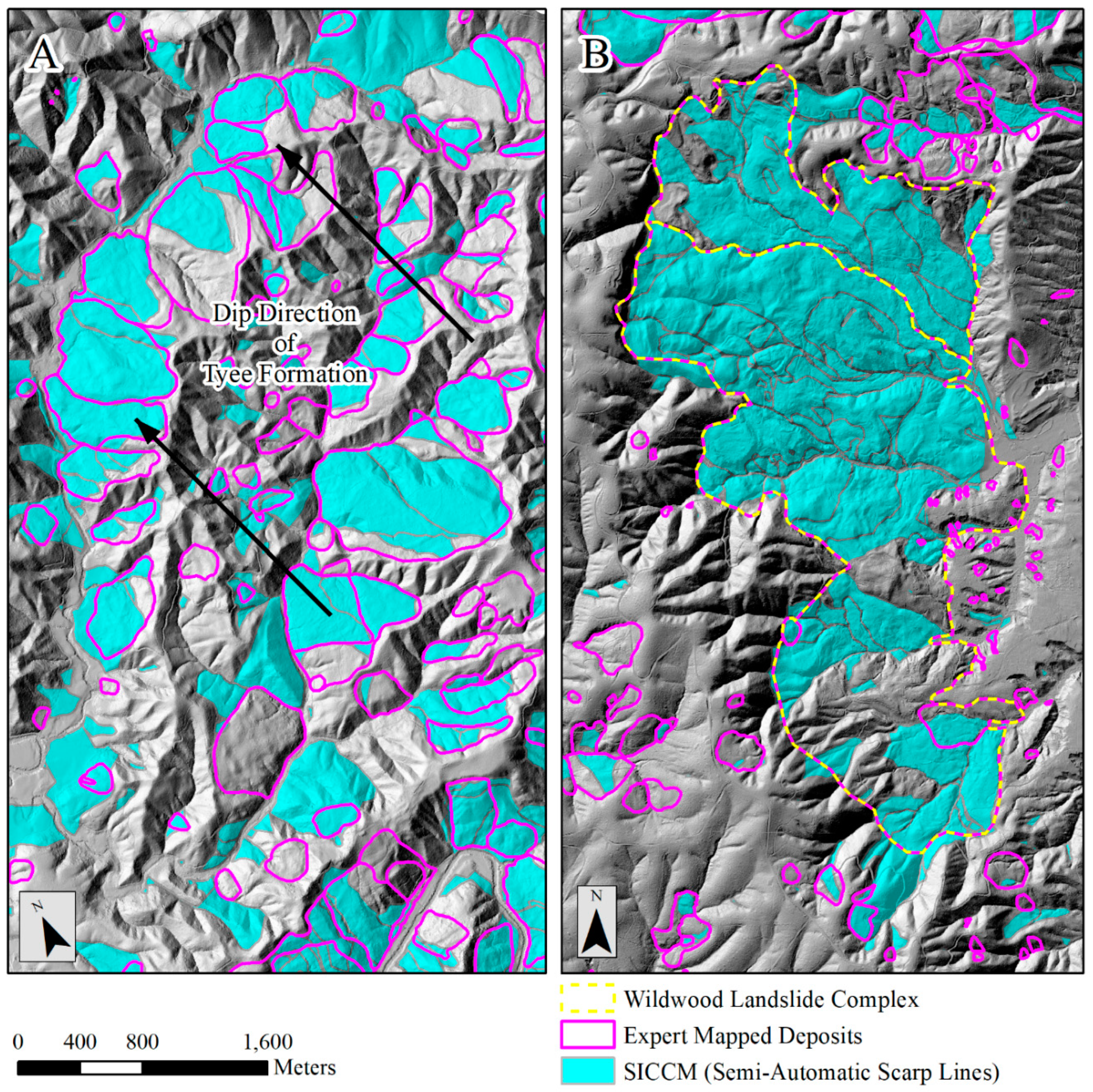
4.4. Influence of Geology on SICCM Performance

As described earlier, several study areas were used to evaluate the influence of geology on SICCM performance. A summary of the results shown in Figure 11B indicates that accuracy assessment measures were similar for most lithologies considered. Only precision and recall for landslides occurring in surficial sediments, which only occur at Dixie Mountain, varied substantially. Surficial sediments are the primary unstable lithology at Dixie Mountain, as they account for 63 percent of the land area but comprise 94 percent of landslide deposits area. This relationship indicates that the Dixie Mountain results in Figure 11A are nearly equivalent to surficial sediment results in Figure 11B, and the difference in recall is likely explained during the earlier discussion of the Dutch Canyon Complex. The enormity of the Dutch Canyon Complex likely also accounts for the change in precision. Of all three study areas, expertly mapped landslide deposits occupy the greatest proportion of land area in Dixie Mountain, which means that if SICCM maps a deposit somewhere, it is statistically more likely to correspond with an expert deposit. This observation would also mean that Big Elk Creek would have better precision than Gales Creek, which is, in fact, the case. Dixie Mountain, however, has significantly higher precision than the other two study areas, despite having a relatively close proportion of landslide deposits as Big Elk Creek (39 to 33 percent). Precision does appear to be a function of what proportion of an area is mapped as landslides, but the Dixie Mountain results are exacerbated by the distinct differences in terrain, where land is either rough (surficial deposits) and mapped as landslides, or it is smooth (volcanics mantled with loess) and not mapped as landslides. These observations about geology illustrate that geology does influence how SICCM maps an area, but this occurs primarily because geology has an effect on the geomorphology of an area. SICCM’s performance does not appear to be dependent on any geology, as illustrated by lithology.

5. Conclusions

This paper presents a new method for semi-automatically producing landslide inventories called the Scarp Identification and Contour Connection Method (SICCM). SICCM is a two-step process that maps landslide scarps and then implements a modified version of the Leshchinsky et al. [30] Contour Connection Method (CCM) to map landslide deposits. The method was evaluated at three locations within western Oregon, the Dixie Mountain, and Gales Creek quadrangles, and the Big Elk Creek watershed, each with a unique geologic setting. Qualitative and quantitative assessments were made from the results, yielding the following conclusions:

• SICCM produces landslide deposit inventories that yield some of the key knowledge made available by detailed, but also very time consuming, expert-produced landslide inventory. Deposits that were mapped in Dixie Mountain and Big Elk Creek were shown to be capable of identifying regional landslide distributions and variations in geologic structure. Quantitative analyses using SICCM results provide insight into trends of landslide activity, such as the slope, orientation, and size of landslides in an area.
• Despite the requirement of several input parameters, SICCM produced consistent results for all three study areas using the same input parameters. When model parameters were changed, results changed in a controlled, predictable fashion.
• All processes, from producing scarp lines to mapping deposits, involve simplifications of more complex alternatives to SICCM that facilitates human expert involvement and understanding of outputs.
• The diverse geology of the three study areas did not appear to affect the performance of SICCM at mapping landslide deposits. Instead, other factors, such as the proportion of area mapped as deposits or mapped as a specific geologic unit, account for most variability with results.

Several important limitations of mapping deposits with SICCM exist. First, like any semi-automated method, SICCM is dependent on the quality of the input topographic data. Performance is reduced for terrain with significant anthropogenic features, which lead to false scarp identification, and for terrain where weathering has diminished the appearance of landslide scarps. Second, the method has only been designed to map landslides with intact scarp and deposit features. These landslide types generally include rotational and translational slides and do not include debris flows or rockfall-related failures.

References

1. Brardinoni, F.; Slaymaker, O.; Hassan, M.A. Landslide inventory in a rugged forested watershed: A comparison between air-photo and field survey data. Geomorphology 2003, 54, 179–196. [Google Scholar] [CrossRef]
2. Burns, W.J.; Duplantis, S.; Jones, C.B.; English, J.T. LIDAR Data and Landslide Inventory Maps of the North Fork Siuslaw River and Big Elk Creek Watersheds, Lane, Lincoln, and Benton Counties, Oregon; Oregon Department of Geology and Mineral Industries: Portland, OR, USA, 2012.
3. Hofmeister, R.J. Slope Failures in Oregon GIS Inventory for three 1996/97 Storm events. Oregon Dep. Geol. Miner. Ind. 2000, 34, 20. [Google Scholar]
4. Guzzetti, F.; Cardinali, M.; Reichenbach, P.; Cipolla, F.; Sebastiani, C.; Galli, M.; Salvati, P. Landslides triggered by the 23 November 2000 rainfall event in the Imperia Province, Western Liguria, Italy. Eng. Geol. 2004, 73, 229–245. [Google Scholar] [CrossRef]
5. Harp, E.L.; Jibson, R.W. Inventory of Landslides Triggered by the 1994 Northridge, California Earthquake. Bull. Seismol. Soc. Am. 1996, 86, S319–S332. [Google Scholar]
6. Xu, C.; Xu, X.; Yao, X.; Dai, F. Three (nearly) complete inventories of landslides triggered by the May 12, 2008 Wenchuan Mw 7.9 earthquake of China and their spatial distribution statistical analysis. Landslides 2014, 11, 441–461. [Google Scholar] [CrossRef]
7. Tang, C.; Zhu, J.; Qi, X.; Ding, J. Landslides induced by the Wenchuan earthquake and the subsequent strong rainfall event: A case study in the Beichuan area of China. Eng. Geol. 2011, 122, 22–33. [Google Scholar] [CrossRef]
8. Malamud, B.D.; Turcotte, D.L.; Guzzetti, F.; Reichenbach, P. Landslide inventories and their statistical properties. Earth Surf. Process. Landf. 2004, 29, 687–711. [Google Scholar] [CrossRef]
9. Burns, W.J.; Mickelson, K.A. DOGAMI Special Paper 48, Protocol for Deep Landslide Susceptibility Mapping; Oregon Department of Geology and Mineral Industries: Portland, OR, USA, 2016.
10. Hess, D.M.; Leshchinsky, B.A.; Bunn, M.; Benjamin Mason, H.; Olsen, M.J. A simplified three-dimensional shallow landslide susceptibility framework considering topography and seismicity. Landslides 2017, 14, 1677–1697. [Google Scholar] [CrossRef]
11. Mahalingam, R.; Olsen, M.J.; O’Banion, M.S. Evaluation of landslide susceptibility mapping techniques using LIDAR-derived conditioning factors (Oregon case study). Geomat. Nat. Hazards Risk 2016, 7, 1884–1907. [Google Scholar] [CrossRef]
12. Wieczorek, G.F. Preparing a Detailed Landslide-Inventory Map for Hazard Evaluation and Reduction. Environ. Eng. Geosci. 1984, xxi, 337–342. [Google Scholar] [CrossRef]
13. Cruden, D.M.; Varnes, D.J. Landslide types and processes. In Turn. AK, Schuster, RL Landslides Investig. Mitigation, Spec. Rep. 247; Tansportation Research Board: Washington, DC, USA, 1996; pp. 36–75. [Google Scholar]
14. Wills, C.J.; McCrink, T.P. Comparing landslide inventories: The map depends on the method. Environ. Eng. Geosci. 2002, 8, 279–293. [Google Scholar] [CrossRef]
15. Van Den Eeckhaut, M.; Poesen, J.; Verstraeten, G.; Vanacker, V.; Moeyersons, J.; Nyssen, J.; van Beek, L.P.H. The effectiveness of hillshade maps and expert knowledge in mapping old deep-seated landslides. Geomorphology 2005, 67, 351–363. [Google Scholar] [CrossRef]
16. Van Den Eeckhaut, M.; Poesen, J.; Verstraeten, G.; Vanacker, V.; Nyssen, J.; Moeyersons, J.; van Beek, L.P.H.; Vandekerckhove, L. Use of LIDAR-derived images for mapping old landslides under forest. Earth Surf. Process. Landf. 2007, 32, 754–769. [Google Scholar] [CrossRef]
17. Schulz, W.H. Landslides Mapped Using LIDAR Imagery; United States Geological Survey: Seattle, WA, USA, 2004; Volume 4.
18. Ortuño, M.; Guinau, M.; Calvet, J.; Furdada, G.; Bordonau, J.; Ruiz, A.; Camafort, M. Potential of airborne LIDAR data analysis to detect subtle landforms of slope failure: Portainé, Central Pyrenees. Geomorphology 2017, 295, 364–382. [Google Scholar] [CrossRef]
19. Burns, W.J.; Madin, I.P. Protocol for Inventory Mapping of Landslide Deposits from Light Detection and Ranging (LIDAR) Imagery; Oregon Department of Geology and Mineral Industries: Portland, OR, USA, 2009.
20. McKean, J.; Roering, J. Objective landslide detection and surface morphology mapping using high-resolution airborne laser altimetry. Geomorphology 2004, 57, 331–351. [Google Scholar] [CrossRef]
21. Berti, M.; Corsini, A.; Daehne, A. Comparative analysis of surface roughness algorithms for the identification of active landslides. Geomorphology 2013, 182, 1–18. [Google Scholar] [CrossRef]
22. Korzeniowska, K.; Pfeifer, N.; Landtwing, S. Mapping gullies, dunes, lava fields, and landslides via surface roughness. Geomorphology 2018, 301, 53–67. [Google Scholar] [CrossRef]
23. Shi, W.; Deng, S.; Xu, W. Extraction of multi-scale landslide morphological features based on local Gi* using airborne LIDAR-derived DEM. Geomorphology 2018, 303, 229–242. [Google Scholar] [CrossRef]
24. Booth, A.M.; Roering, J.J.; Perron, J.T. Automated landslide mapping using spectral analysis and high-resolution topographic data: Puget Sound lowlands, Washington, and Portland Hills, Oregon. Geomorphology 2009, 109, 132–147. [Google Scholar] [CrossRef]
25. Glenn, N.F.; Streutker, D.R.; Chadwick, D.J.; Thackray, G.D.; Dorsch, S.J. Analysis of LIDAR-derived topographic information for characterizing and differentiating landslide morphology and activity. Geomorphology 2006, 73, 131–148. [Google Scholar] [CrossRef]
26. Van Den Eeckhaut, M.; Kerle, N.; Poesen, J.; Hervás, J. Object-oriented identification of forested landslides with derivatives of single pulse LIDAR data. Geomorphology 2012, 173–174, 30–42. [Google Scholar] [CrossRef]
27. Chen, W.; Li, X.; Wang, Y.; Chen, G.; Liu, S. Forested landslide detection using LIDAR data and the random forest algorithm: A case study of the Three Gorges, China. Remote Sens. Environ. 2014, 152, 291–301. [Google Scholar] [CrossRef]
28. Li, X.; Cheng, X.; Chen, W.; Chen, G.; Liu, S. Identification of forested landslides using LIDAR data, object-based image analysis, and machine learning algorithms. Remote Sens. 2015, 7, 9705–9726. [Google Scholar] [CrossRef]
29. Pawłuszek, K.; Borkowski, A. Landslides Identification Using Airborne Laser Scanning Data Derived Topographic Terrain Attributes and Support Vector Machine Classification. ISPRS Int. Arch. Photogramm. Remote Sens. Spat. Inf. Sci. 2016, XLI-B8, 145–149. [Google Scholar] [CrossRef]
30. Leshchinsky, B.A.; Olsen, M.J.; Tanyu, B.F. Contour Connection Method for automated identification and classification of landslide deposits. Comput. Geosci. 2015, 74, 27–38. [Google Scholar] [CrossRef]
31. Highland, L.M.; Bobrowsky, P. The Landslide Handbook—A Guide to Understanding Landslides. Available online: https://pubs.usgs.gov/circ/1325/ (accessed on 9 October 2018).
32. Booth, A.M.; LaHusen, S.R.; Duvall, A.R.; Montgomery, D.R. Holocene history of deep-seated landsliding in the North Fork Stillaguamish River valley from surface roughness analysis, radiocarbon dating, and numerical landscape evolution modeling. JGR Earth Surf. 2017, 122, 456–472. [Google Scholar] [CrossRef]
33. Lashermes, B.; Foufoula-Georgiou, E.; Dietrich, W.E. Channel network extraction from high resolution topography using wavelets. Geophys. Res. Lett. 2007, 34. [Google Scholar] [CrossRef] [Green Version]
34. Roering, J.J.; Marshall, J.; Booth, A.M.; Mort, M.; Jin, Q. Evidence for biotic controls on topography and soil production. Earth Planet. Sci. Lett. 2010, 298, 183–190. [Google Scholar] [CrossRef]
35. Burrough, P.; McDonnell, R.A. Principles of Geographical Information Systems; Oxford University Press: London, UK, 1998; Volume 330. [Google Scholar] [CrossRef]
36. Zevenbergen, L.W.; Thorne, C.R. Quantitative Analysis of Land Surface Topography. Earth Surf. Process. Landf. 1987, 12, 47–56. [Google Scholar] [CrossRef]
37. Gaidzik, K.; Ramírez-Herrera, M.T.; Bunn, M.; Leshchinsky, B.A.; Olsen, M.; Regmi, N.R. Landslide manual and automated inventories, and susceptibility mapping using LIDAR in the forested mountains of Guerrero, Mexico. Geomat. Nat. Hazards Risk 2017, 8. [Google Scholar] [CrossRef]
38. De Smith, M.J.; Goodchild, M.F.; Longley, P.A.; De Smith, M.J. Geospatial Analysis; Matador: Leicester, UK, 2015; ISBN 1905886608. [Google Scholar]
39. O’Callaghan, J.F.; Mark, D.M. The extraction of drainage networks from digital elevation data. Comput. Vis. Graph. Image Process. 1984, 27, 247. [Google Scholar] [CrossRef]
40. Zhan, C. A Hybrid Line Thinning Approach. In Auto-Carto 11; American Society for Photogrammetry and Remote Sensing: Minneapolis, MN, USA, 1993; pp. 396–405. [Google Scholar]
41. Perry, J.W.; Kent, A.; Berry, M.M. Machine literature searching X. Machine language; factors underlying its design and development. Am. Doc. 1955, 6, 242–254. [Google Scholar] [CrossRef]
42. LIDAR Remote Sensing Data Collection: Department of Geology & Mineral Industries, Oregon Department of Forestry, Puget Sound LIDAR Consortium; Oregon Department of Geology and Mineral Industries: Portland, OR, USA, 2007.
43. LIDAR Remote Sensing Data Collection: Department of Geology and Mineral Industries Central Coast Study Area; Oregon Department of Geology and Mineral Industries: Portland, OR, USA, 2012.
44. Burns, W.J.; Mickelson, K.A.; Duplantis, S.; Madin, I.P. IMS-44, Landslide Inventory Maps of the Dixie Mountain Quadrangle, Washington, Multnomah, and Columbia Counties, Oregon; Nature of the Northwest Information Center: Portland, OR, USA, 2012.
45. Burns, W.J.; Duplantis, S.; Mickelson, K.A. IMS-46, Landslide Inventory Maps of the Gales Creek Quadrangle, Washington County, Oregon; Nature of the Northwest Information Center: Portland, OR, USA, 2012. [Google Scholar]
46. Madin, I.P.; Niewendorp, C.A. Preliminary Geologic Map of the Dixie Mountain 7.5’ Quadrangle, Columbia, Multnomah, and Washington Counties, Oregon; Oregon Department of Geology and Mineral Industries: Portland, OR, USA, 2008.
47. Yeats, R.S.; Graven, E.P.; Werner, K.S.; Goldfinger, C.; Popowski, T.A. Tectonics of the Willamette Valley, Oregon. In Assessing Earthquake Hazards and Reducing Risk in the Pacific Northwest; Volume I; Rogers, A.M., Walsh, T.J., Kockleman, W.J., Priest, G.R., Eds.; United States Geological Survey: Reston, VA, USA, 1996; pp. 183–222. [Google Scholar]
48. McClaughry, J.D.; Wiley, T.J.; Ferns, M.L.; Madin, I.P. Digital Geologic Map of the Southern Willamette Valley, Benton, Lane, Linn, Marion, and Polk Counties, Oregon; Oregon Department of Geology and Mineral Industries: Portland, OR, USA, 2010.
49. Smith, R.L.; Roe, W.P. Oregon Geologic Data Compilation (OGDC), Release 6; Oregon Department of Geology and Mineral Industries: Portland, OR, USA, 2015.
Figure 1. Appearance of (A) faceted terrain and (B) topographic lumps, and their relationship with LIDAR ground point density. The point density raster has been resampled from its initial 1-m cell size to a 5-m cell size to emphasize areas with high or low point density.
Remotesensing 11 00303 g001
Figure 2. Change in digital elevation model (DEM) appearance associated with resampling to a higher cell size. Images include hillshade and contour maps derived from the original DEM (A,B,D,E), and contour maps produced from the resampled DEM (C,F). The top row (AC) focuses on unwanted features, while the bottom row (DF) focuses on landslide features.
Remotesensing 11 00303 g002
Figure 3. Illustration of the four primary steps used to identify scarp lines from a DEM: (1) compute mixture raster, (2) produce scarp polygon candidates from mixture raster, (3) classify scarp polygon candidates, and (4) convert scarp polygons into scarp lines.
Remotesensing 11 00303 g003
Figure 4. Comparison of Burns and Madin (2009) and SICCM definitions of a scarp line.
Remotesensing 11 00303 g004
Figure 5. Distribution of mixture raster values for the Big Elk Creek watershed, showing the location of the mixture threshold.
Remotesensing 11 00303 g005
Figure 6. The steps involved with SICCM: (A) start with elevation raster, (B) locate scarp line, (C) draw region of interest around scarp line, (D) focus analysis on the region of interest, (E) draw elevation contours at interval ΔEz, (F) draw nodes equally spaced by Ln on contours, (G) connect nodes on adjacent contours and evaluate Δactive and Bn, (H) draw landslide deposit extents around successful connections.
Remotesensing 11 00303 g006
Figure 7. Process used to define search area for landslide deposit mapping from scarp lines.
Remotesensing 11 00303 g007
Figure 8. Geologic overview of the three study areas, and their location within the state of Oregon. Expert mapped landslides are shown to illustrate their distribution in each study area.
Remotesensing 11 00303 g008
Figure 9. Study area inventories produced by SICCM using automatic scarp lines. Expert mapped deposits for the (A) Dixie Mountain quadrangle [44], (B) Gales Creek quadrangle [45], and (C) Big Elk Creek watershed [2] are included for comparison.
Remotesensing 11 00303 g009
Figure 10. Study area inventories produced by SICCM using semi-automatic scarp lines. Expert mapped deposits for the (A) Dixie Mountain quadrangle [44], (B) Gales Creek quadrangle [45], and (C) Big Elk Creek watershed [2] are included for comparison.
Remotesensing 11 00303 g010
Figure 11. SICCM accuracy assessment divided by (A) study area location and (B) generalized lithological unit.
Remotesensing 11 00303 g011
Figure 12. Comparison of SICCM and expert mapped deposits for (A) the Tyee Formation in Big Elk Creek, and (B) the Wildwood Landslide Complex in the Dixie Mountain Quadrangle.
Remotesensing 11 00303 g012
Figure 13. Focused view on the Dutch Canyon Complex, Dixie Mountain. A large and highly eroded main scarp explains why SICCM significantly under-mapped the complex.
Remotesensing 11 00303 g013
Figure 14. Automatic SICCM inventory for the Big Elk Creek watershed showing the distribution of landslides variation in landslide slope aspect. Geologic folds are taken from Smith and Roe [49].
Remotesensing 11 00303 g014
Figure 15. Comparison of slopes within SICCM deposits to all slopes within the Big Elk Creek watershed.
Remotesensing 11 00303 g015
Figure 16. Sensitivity of SICCM results to the cell size used in scarp line identification. The plots display accuracy assessment results obtained after performing automatic scarp line identification at three different cell sizes for the (A) Big Elk Creek watershed, (B) Dixie Mountain quadrangle, and (C) Gales Creek quadrangle.
Remotesensing 11 00303 g016
Figure 17. Sensitivity of validation measures to variations in deposit mapping parameter values. Results of each plot were produced using Bn = 5, Δactive = 2°, Ln = 6 m, ΔEz = 6 m, with only the stated parameter being varied.
Remotesensing 11 00303 g017
Figure 18. Sensitivity of deposit shapes to input parameters. Parameters are symbolized in the text as contour interval, ΔEz; node spacing, Ln; branch parameter, Bn; and active slope, Δactive. Changes in active slope did not change the appearance of the landslide in the first three rows and a new landslide was selected for the final row.
Remotesensing 11 00303 g018