Monitoring Landscape Dynamics in Central U.S. Grasslands with Harmonized Landsat-8 and Sentinel-2 Time Series Data

 , , , , , and
Abstract
:1. Introduction
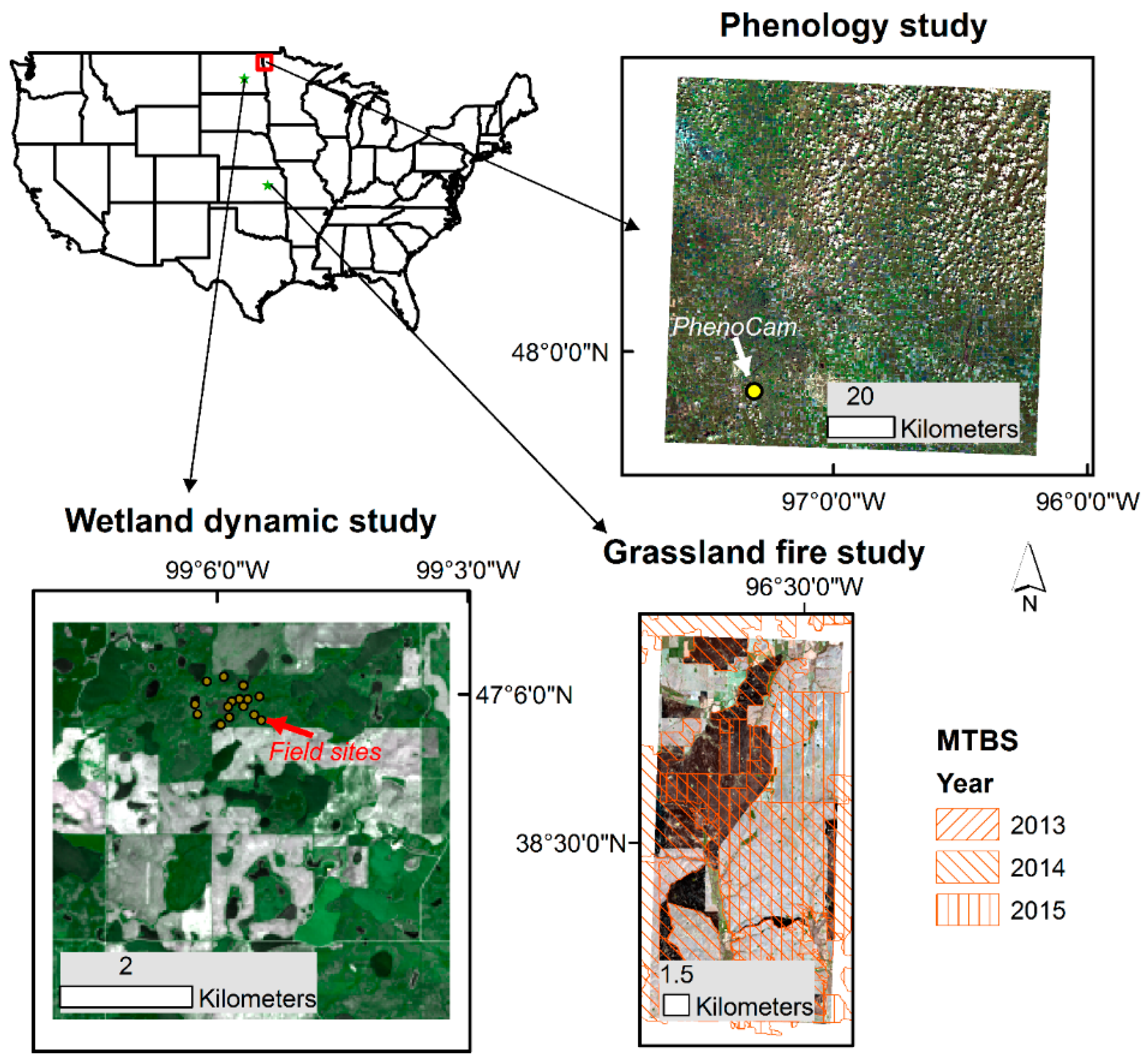
2. Study Area
2.1. Vegetation Phenology
2.2. Grassland Fire
2.3. Wetland Dynamics
3. Source Data
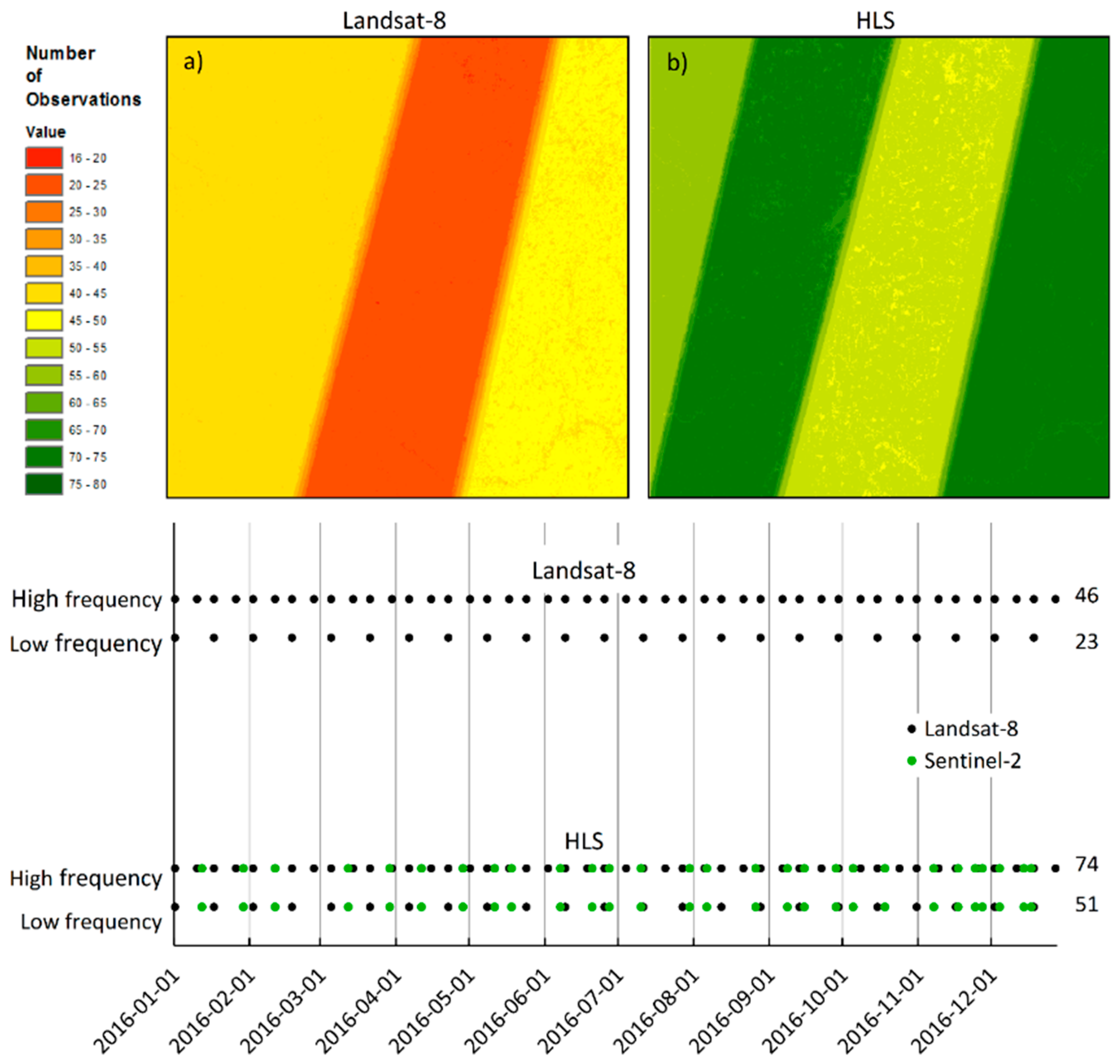
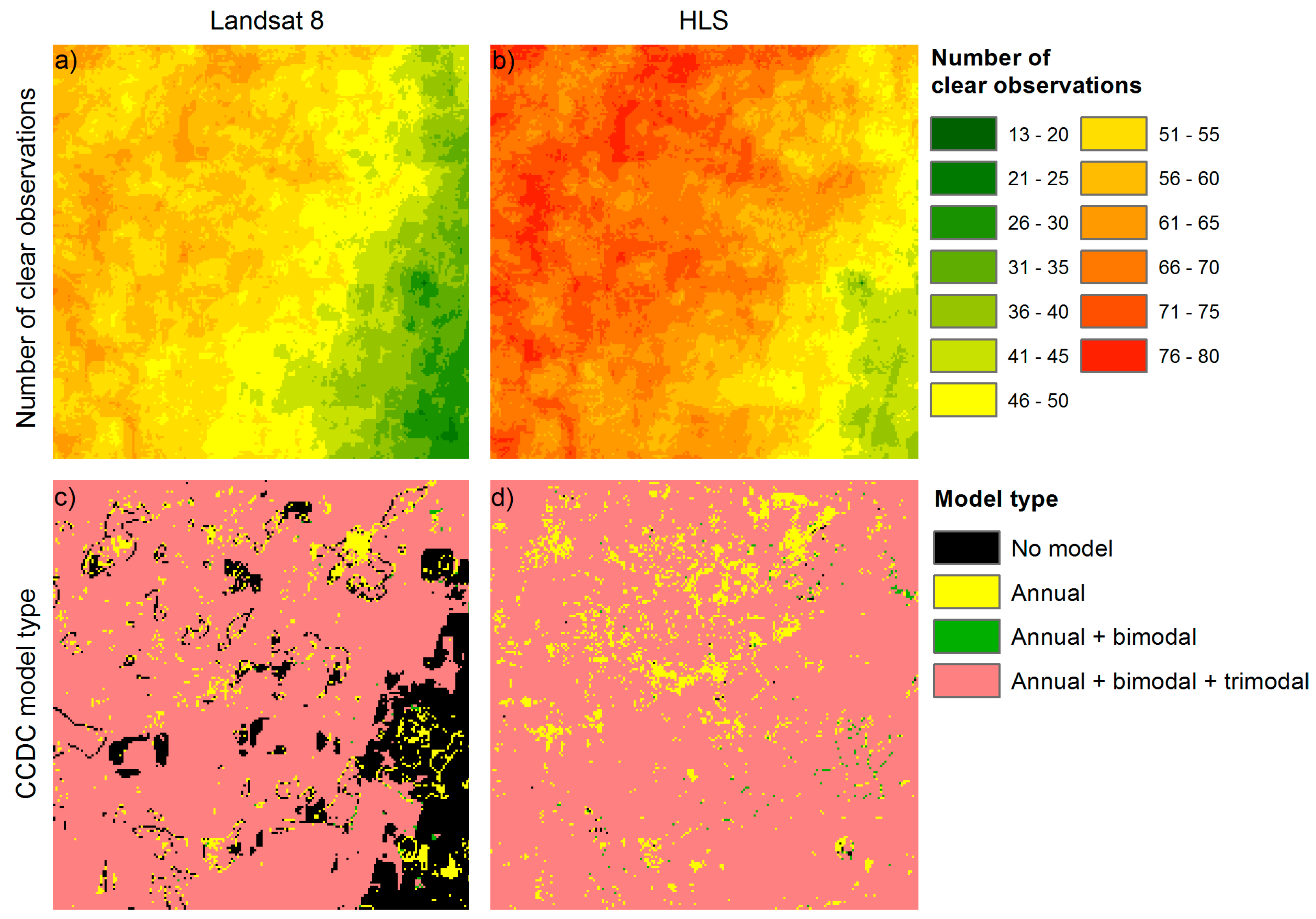
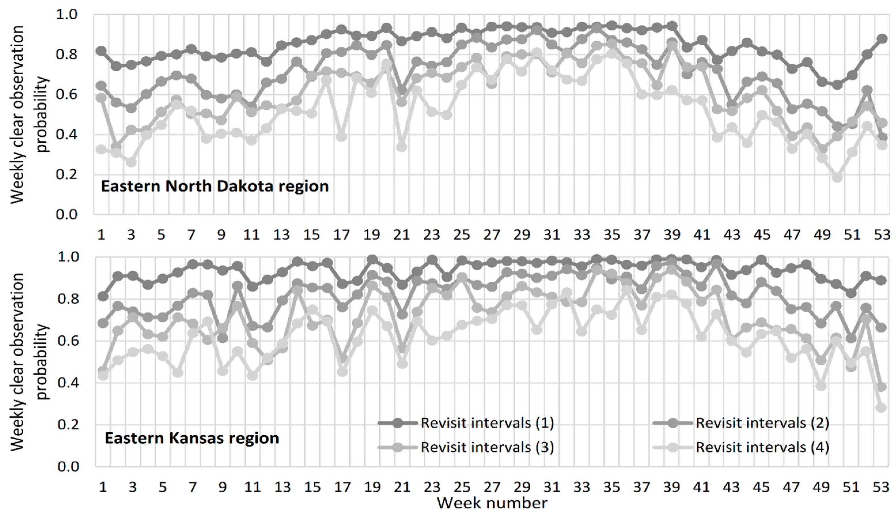
3.1. Harmonized Landsat-8 and Sentinel-2 (HLS)
3.2. Reference Data for the Vegetation Phenology Analyses
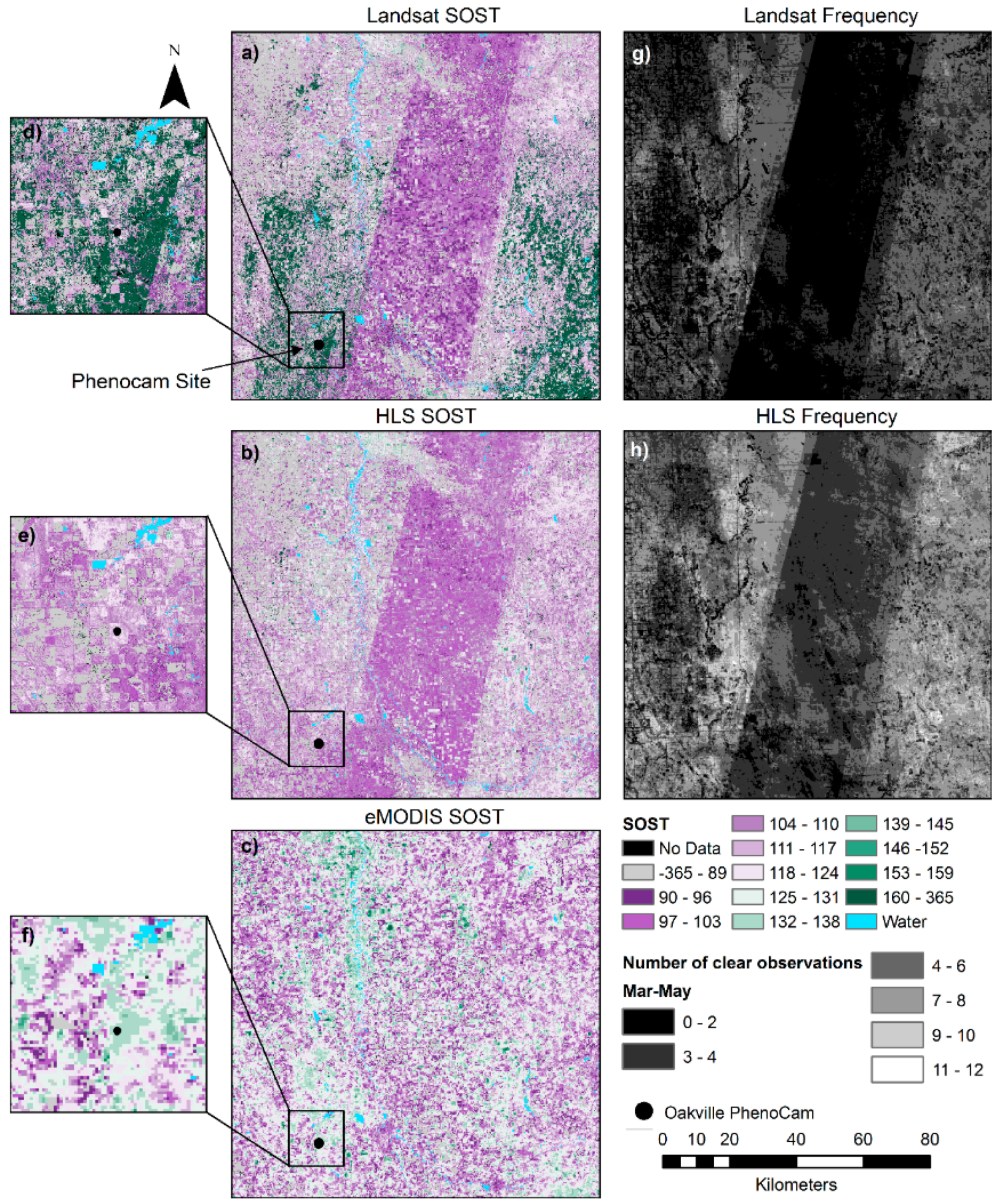
3.2.1. Oakville PhenoCam
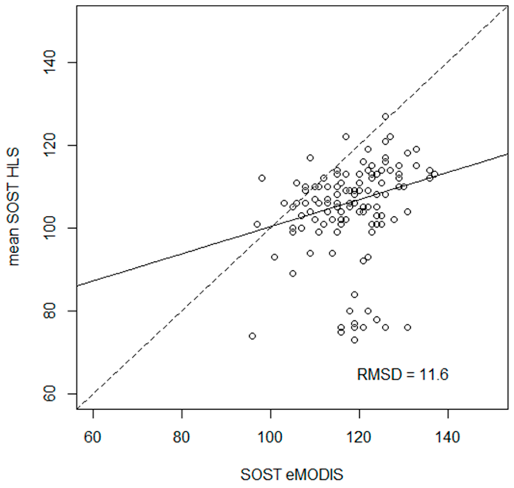
3.2.2. eMODIS NDVI and Phenology Metrics
3.2.3. CDL and NLCD
3.3. Reference Data for the Grassland Fire Analyses
3.3.1. Monitoring Trends in Burn Severity (MTBS)
3.3.2. Burned Area Essential Climate Variable (BAECV)
3.4. Reference Data for the Wetland Dynamics Analyses
3.4.1. Climate Data
3.4.2. Water Surface Elevation Data
4. Methods
4.1. Phenology
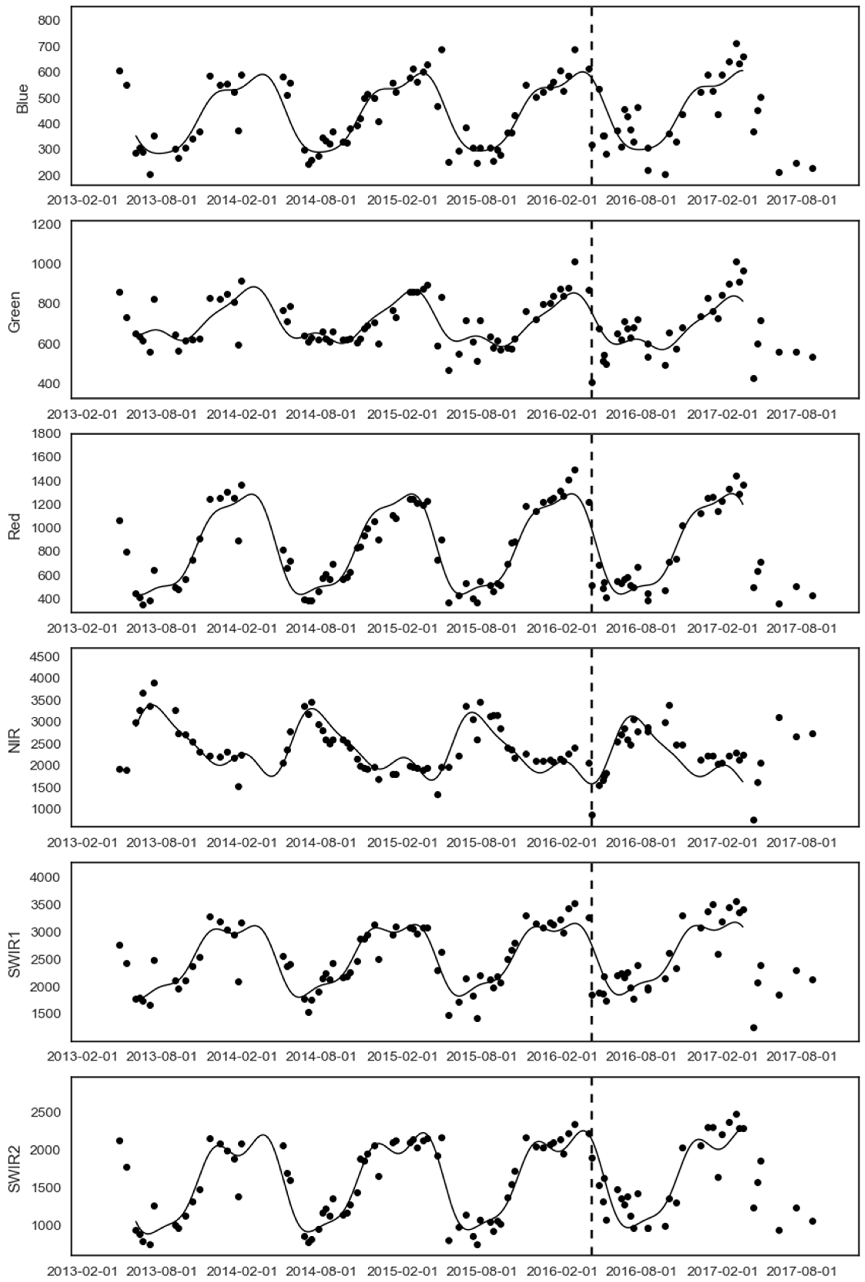
4.2. Detecting Burn Scars from Grassland Fires
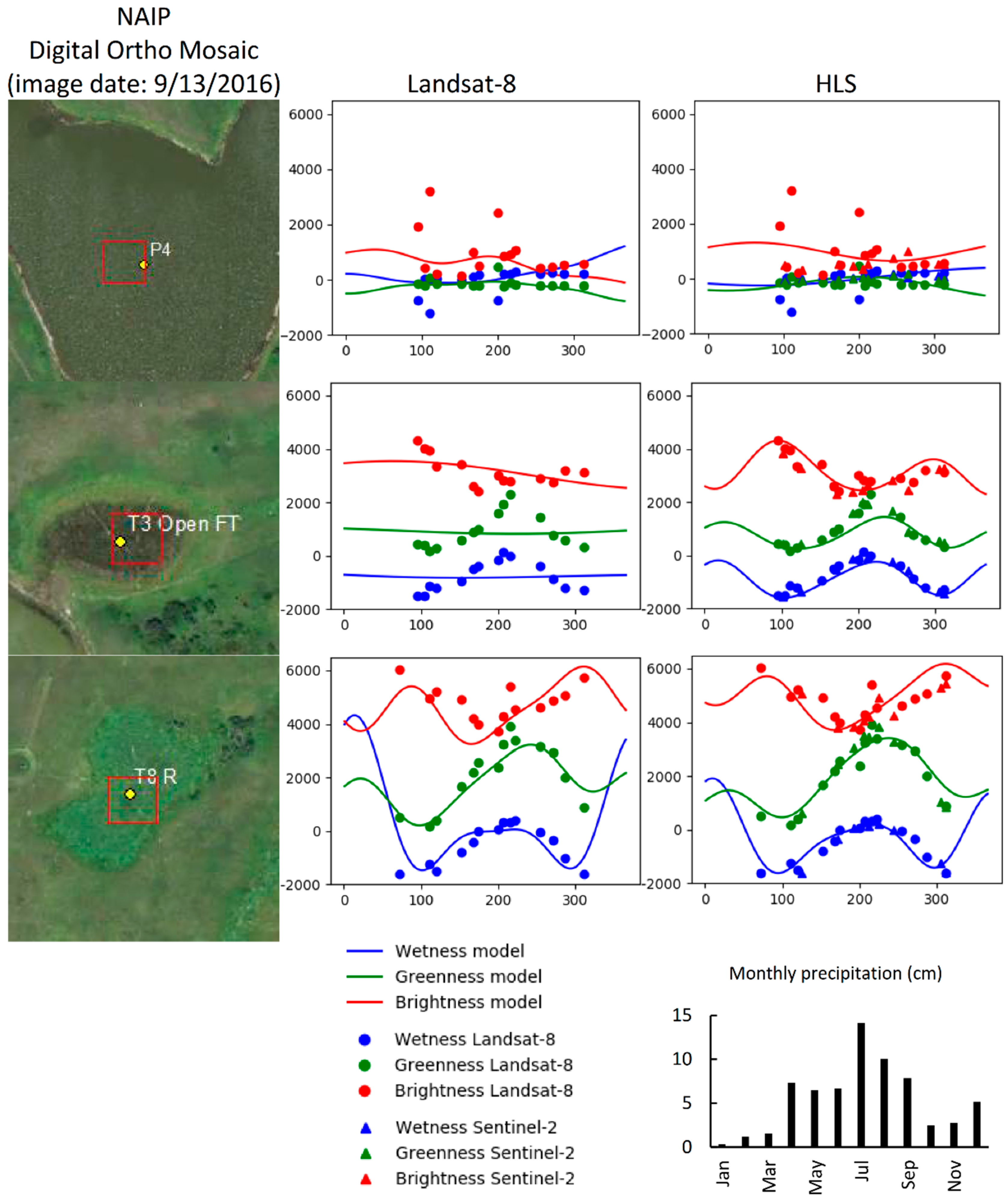
4.3. Characterizing Seasonal Wetland Dynamics
5. Results
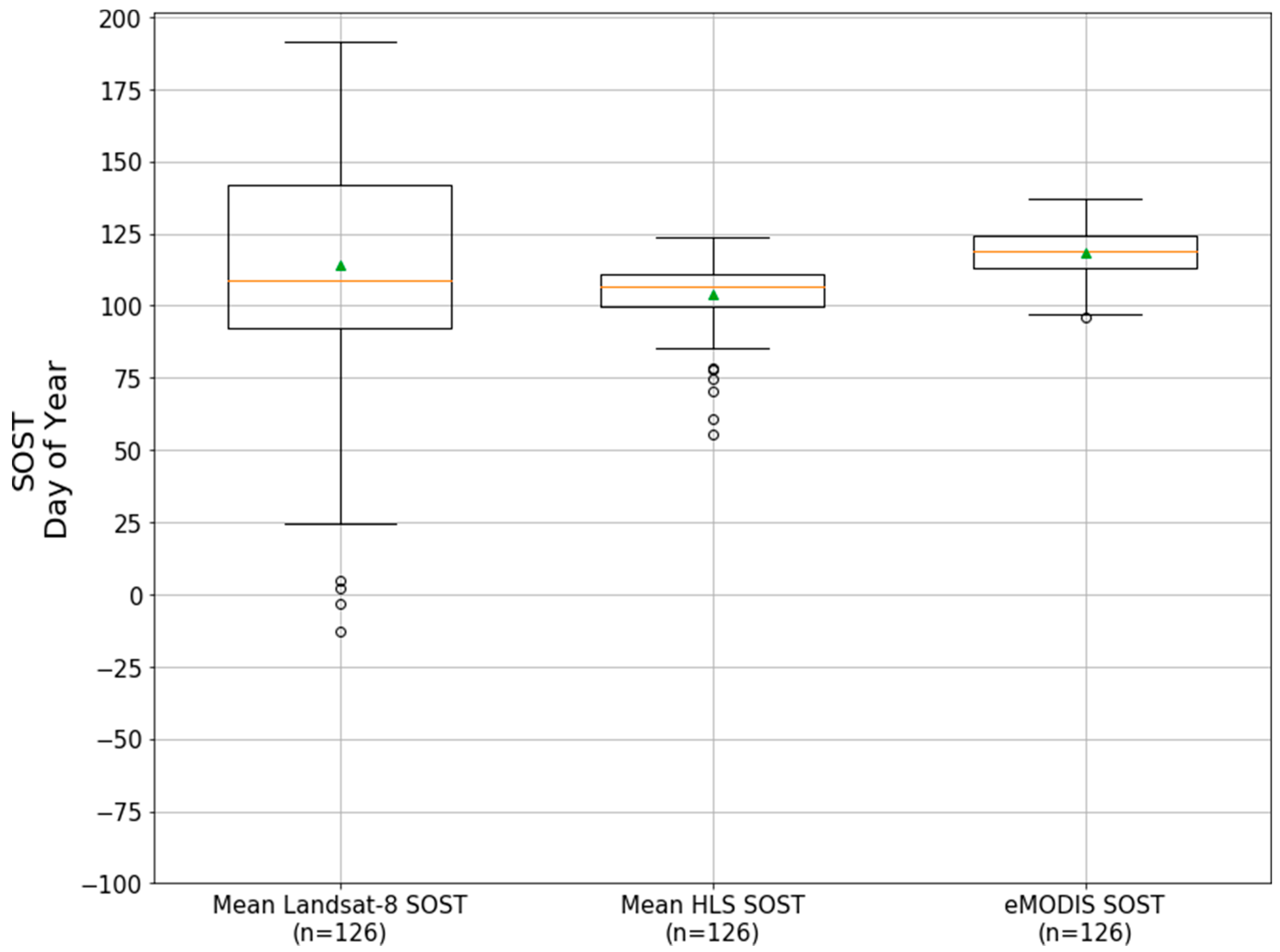
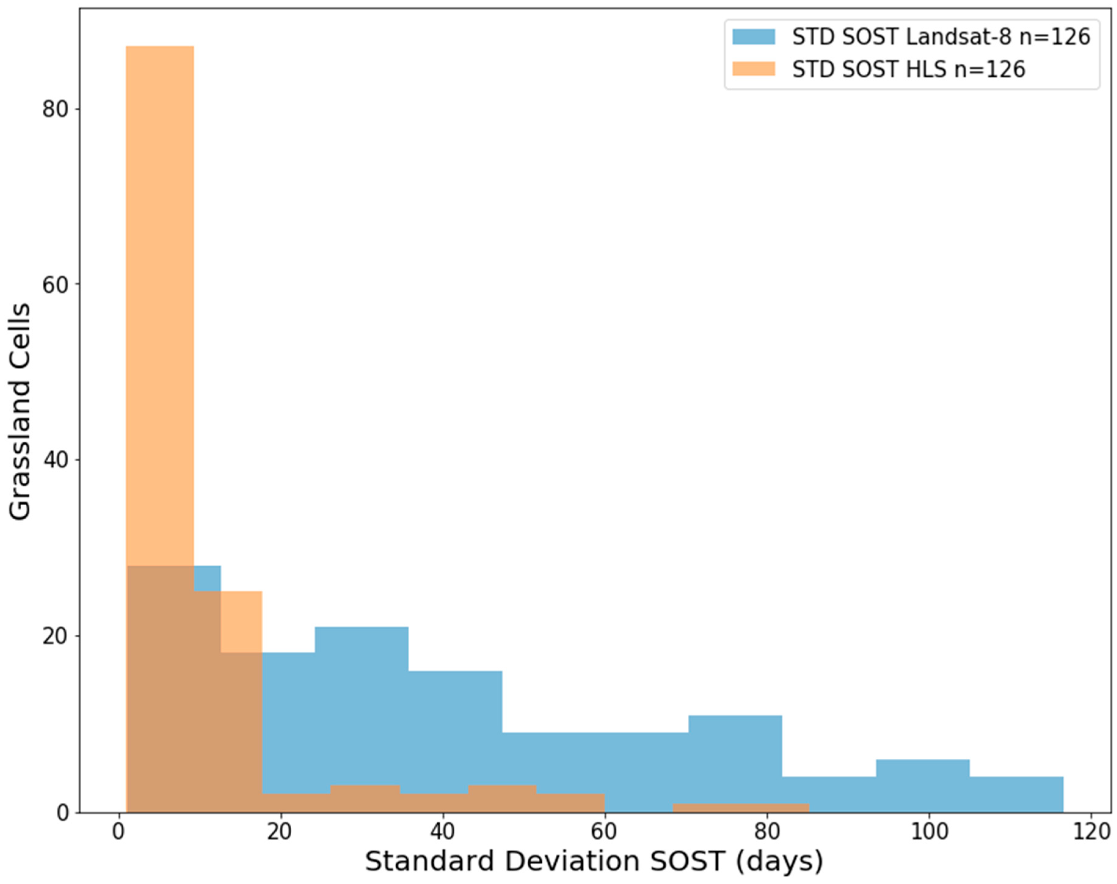
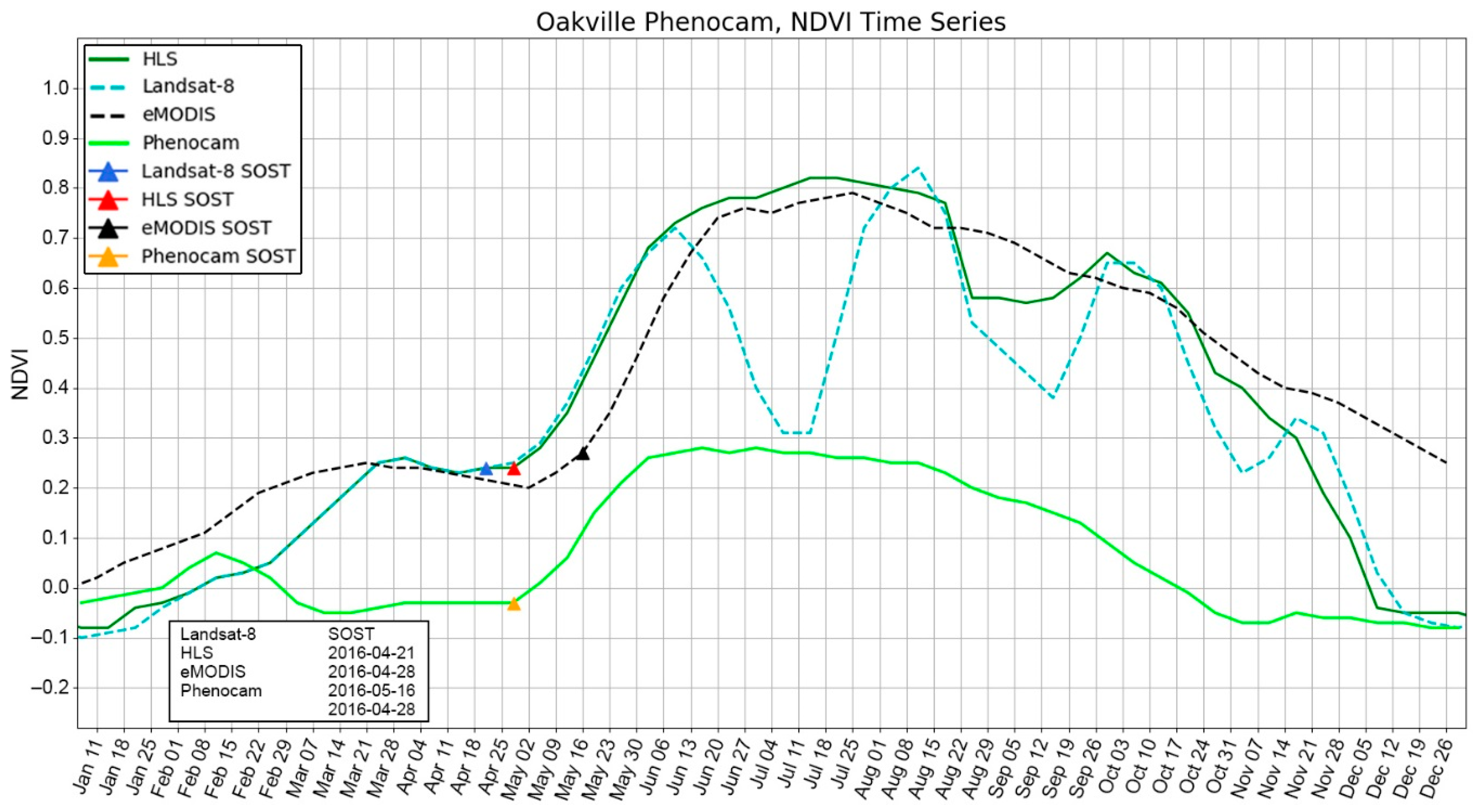
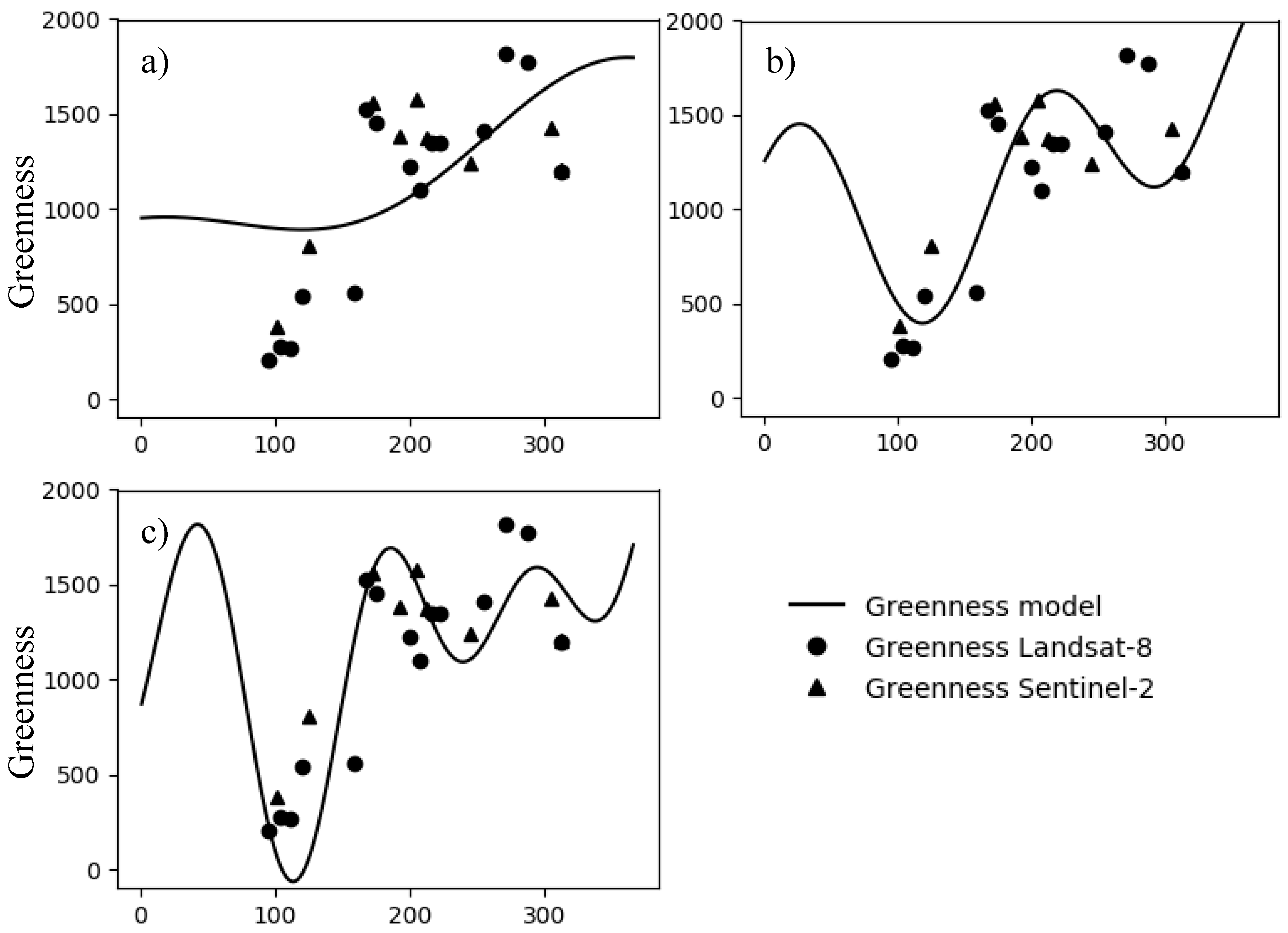
5.1. Phenology
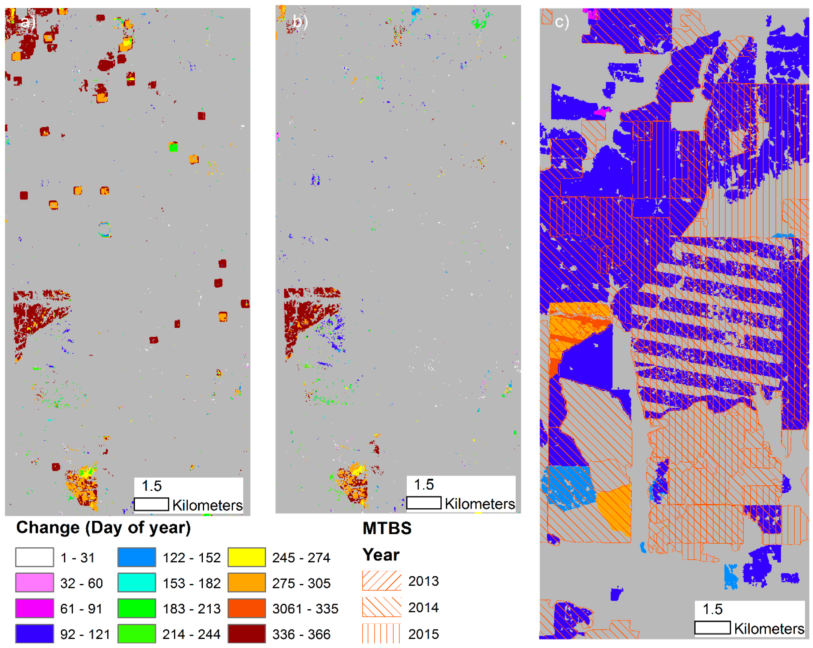
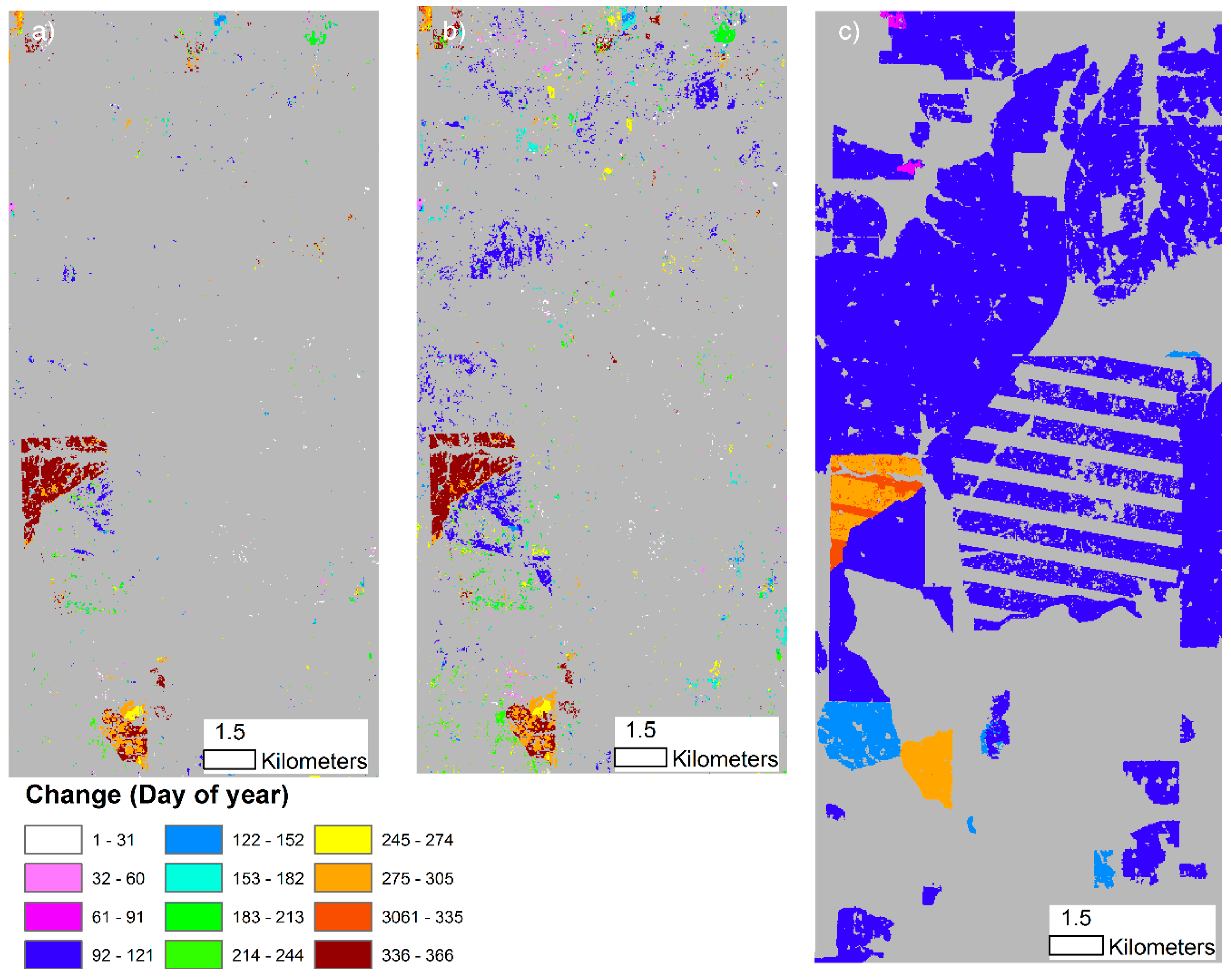
5.2. Grassland Fires
5.3. Wetland Dynamics
6. Discussion
7. Conclusions
Author Contributions
Funding
Acknowledgments
Conflicts of Interest
Appendix A


References
- Drummond, M.A.; Auch, R.F.; Karstensen, K.A.; Sayler, K.L.; Taylor, J.L.; Loveland, T.R. Land change variability and human–environment dynamics in the United States Great Plains. Land Use Policy 2012, 29, 710–723. [Google Scholar] [CrossRef]
- Euliss, N.H., Jr.; Gleason, R.; Olness, A.; McDougal, R.; Murkin, H.; Robarts, R.; Bourbonniere, R.; Warner, B. North American prairie wetlands are important nonforested land-based carbon storage sites. Sci. Total Environ. 2006, 361, 179–188. [Google Scholar] [CrossRef] [PubMed] [Green Version]
- Euliss, N.H., Jr.; Wrubleski, D.A.; Mushet, D.M. Wetlands of the Prairie Pothole Region: Invertebrate Species Composition, Ecology, and Management; John Wiley and Sons: Hoboken, NJ, USA, 1999. [Google Scholar]
- Lupo, C.D.; Clay, D.E.; Benning, J.L.; Stone, J.J. Life-cycle assessment of the beef cattle production system for the Northern Great Plains, USA. J. Environ. Qual. 2013, 42, 1386–1394. [Google Scholar] [CrossRef] [PubMed]
- Zhu, Z.; Bouchard, M.; Butman, D.; Hawbaker, T.; Li, Z.; Liu, J.; Liu, S.; McDonald, C.; Reker, R.; Sayler, K. Baseline and Projected Future Carbon Storage and Greenhouse-Gas Fluxes in the Great Plains Region of the United States; U.S. Geological Survey: Reston, VA, USA, 2011.
- Higgins, K.F. Interpretation and Compendium of Historical Fire Accounts in the Northern Great Plains; US Fish and Wildlife Service: Washington, DC, USA, 1986. [Google Scholar]
- Johnson, W.C.; Millett, B.V.; Gilmanov, T.; Voldseth, R.A.; Guntenspergen, G.R.; Naugle, D.E. Vulnerability of northern prairie wetlands to climate change. Aibs Bull. 2005, 55, 863–872. [Google Scholar] [CrossRef]
- Twidwell, D.; Rogers, W.E.; Fuhlendorf, S.D.; Wonkka, C.L.; Engle, D.M.; Weir, J.R.; Kreuter, U.P.; Taylor, C.A., Jr. The rising Great Plains fire campaign: Citizens’ response to woody plant encroachment. Front. Ecol. Environ. 2013, 11, e64–e71. [Google Scholar] [CrossRef]
- Brown, J.F. Start of Season Time Dataset. 2018. Available online: https://bit.ly/2takIm0 (accessed on 7 February 2019).
- Chen, Y.; Huang, C.; Ticehurst, C.; Merrin, L.; Thew, P. An evaluation of MODIS daily and 8-day composite products for floodplain and wetland inundation mapping. Wetlands 2013, 33, 823–835. [Google Scholar] [CrossRef]
- Delbart, N.; Le Toan, T.; Kergoat, L.; Fedotova, V. Remote sensing of spring phenology in boreal regions: A free of snow-effect method using NOAA-AVHRR and SPOT-VGT data (1982–2004). Remote Sens. Environ. 2006, 101, 52–62. [Google Scholar] [CrossRef]
- Moulin, S.; Kergoat, L.; Viovy, N.; Dedieu, G. Global-scale assessment of vegetation phenology using NOAA/AVHRR satellite measurements. J. Clim. 1997, 10, 1154–1170. [Google Scholar] [CrossRef]
- White, M.A.; de Beurs, K.M.; Didan, K.; Inouye, D.W.; Richardson, A.D.; Jensen, O.P.; O’KEEFE, J.; Zhang, G.; Nemani, R.R.; van Leeuwen, W.J. Intercomparison, interpretation, and assessment of spring phenology in North America estimated from remote sensing for 1982–2006. Glob. Chang. Biol. 2009, 15, 2335–2359. [Google Scholar] [CrossRef]
- Fisher, J.I.; Mustard, J.F. Cross-scalar satellite phenology from ground, Landsat, and MODIS data. Remote Sens. Environ. 2007, 109, 261–273. [Google Scholar] [CrossRef]
- Yan, L.; Roy, D.P. Large-Area Gap Filling of Landsat Reflectance Time Series by Spectral-Angle-Mapper Based Spatio-Temporal Similarity (SAMSTS). Remote Sens. 2018, 10, 609. [Google Scholar] [CrossRef]
- Claverie, M.; Ju, J.; Masek, J.G.; Dungan, J.L.; Vermote, E.F.; Roger, J.-C.; Skakun, S.V.; Justice, C. The Harmonized Landsat and Sentinel-2 surface reflectance data set. Remote Sens. Environ. 2018, 219, 145–161. [Google Scholar] [CrossRef]
- Fisher, J.I.; Mustard, J.F.; Vadeboncoeur, M.A. Green leaf phenology at Landsat resolution: Scaling from the field to the satellite. Remote Sens. Environ. 2006, 100, 265–279. [Google Scholar] [CrossRef]
- Melaas, E.K.; Friedl, M.A.; Zhu, Z. Detecting interannual variation in deciduous broadleaf forest phenology using Landsat TM/ETM+ data. Remote Sens. Environ. 2013, 132, 176–185. [Google Scholar] [CrossRef]
- Zhang, X.; Friedl, M.; Schaaf, C. Global vegetation phenology from MODIS: Evaluation of global patterns and comparison with in situ measurements. J. Geophys. Res. 2006, 111, G04017. [Google Scholar] [CrossRef]
- Brown, J.F.; Howard, D.; Wylie, B.; Frieze, A.; Ji, L.; Gacke, C. Application-ready expedited MODIS data for operational land surface monitoring of vegetation condition. Remote Sens. 2015, 7, 16226–16240. [Google Scholar] [CrossRef]
- Swets, D.L. A weighted least-squares approach to temporal smoothing of NDVI. In Proceedings of the 1999 ASPRS Annual Conference, from Image to Information, Portland, OR, USA, 17–21 May 1999; American Society for Photogrammetry and Remote Sensing: Bethesda, MD, USA, 1999. [Google Scholar]
- Zhu, Z.; Woodcock, C.E. Continuous change detection and classification of land cover using all available Landsat data. Remote Sens. Environ. 2014, 144, 152–171. [Google Scholar] [CrossRef]
- NOAA. National Centers for Environmental Information; Climate at a Glance: Divisional Time Series; NOAA: Washington, DC, USA, 2018.
- US Department of Agriculture, National Agricultural Statistics Service. Cropland Data Layer. 2016. Available online: https://www.nass.usda.gov/Research_and_Science/Cropland/SARS1a.php (accessed on 2 February 2019).
- Sonnentag, O.; Hufkens, K.; Teshera-Sterne, C.; Young, A.M.; Friedl, M.; Braswell, B.H.; Milliman, T.; O’Keefe, J.; Richardson, A.D. Digital repeat photography for phenological research in forest ecosystems. Agri. For. Meteorol. 2012, 152, 159–177. [Google Scholar] [CrossRef]
- Wilgers, D.; Horne, E. Effects of different burn regimes on tallgrass prairie herpetofaunal species diversity and community composition in the Flint Hills, Kansas. J. Herpetol. 2006, 40, 73–84. [Google Scholar] [CrossRef]
- Eidenshink, J.; Schwind, B.; Brewer, K.; Zhu, Z.-L.; Quayle, B.; Howard, S. A project for monitoring trends in burn severity. Fire Ecol. 2007, 3, 3–21. [Google Scholar] [CrossRef]
- Hawbaker, T.; Stitt, S.; Beal, Y.; Schmidt, G.; Falgout, J.; Williams, B.; Takacs, J. Provisional Burned Area Essential Climate Variable (BAECV) Algorithm Description; The United States Department of the Interior: Washington, DC, USA, 2015.
- LaBaugh, J.W.; Mushet, D.M.; Rosenberry, D.O.; Euliss, N.H.; Goldhaber, M.B.; Mills, C.T.; Nelson, R.D. Changes in pond water levels and surface extent due to climate variability alter solute sources to closed-basin prairie-pothole wetland ponds, 1979 to 2012. Wetlands 2016, 36, 343–355. [Google Scholar] [CrossRef]
- Mushet, D.M.; Rosenberry, D.O.; Euliss, N.H., Jr.; Solensky, M.J. Cottonwood Lake Study Area-Water Surface Elevations; U.S. Geological Survey: Reston, VA, USA, 2016.
- Meier, G.A.; Brown, J.F.; Evelsizer, R.J.; Vogelmann, J.E. Phenology and climate relationships in aspen (Populus tremuloides Michx.) forest and woodland communities of southwestern Colorado. Ecol. Indic. 2015, 48, 189–197. [Google Scholar] [CrossRef]
- Jenkerson, C.; Maiersperger, T.; Schmidt, G. eMODIS: A User-Friendly Data Source; 2331-1258; U.S. Geological Survey: Reston, VA, USA, 2010.
- Homer, C.; Dewitz, J.; Yang, L.; Jin, S.; Danielson, P.; Xian, G.; Coulston, J.; Herold, N.; Wickham, J.; Megown, K. Completion of the 2011 National Land Cover Database for the conterminous United States–representing a decade of land cover change information. Photogramm. Eng. Remote Sens. 2015, 81, 345–354. [Google Scholar]
- Vanderhoof, M.K.; Fairaux, N.; Beal, Y.-J.G.; Hawbaker, T.J. Validation of the USGS Landsat burned area essential climate variable (BAECV) across the conterminous United States. Remote Sens. Environ. 2017, 198, 393–406. [Google Scholar] [CrossRef]
- Baig, M.H.A.; Zhang, L.; Shuai, T.; Tong, Q. Derivation of a tasselled cap transformation based on Landsat 8 at-satellite reflectance. Remote Sens. Lett. 2014, 5, 423–431. [Google Scholar] [CrossRef]
- Roy, D.; Yan, L. Robust Landsat-based crop time series modelling. Remote Sens. Environ. 2018, in press. [Google Scholar] [CrossRef]
- Vrieling, A.; Meroni, M.; Darvishzadeh, R.; Skidmore, A.K.; Wang, T.; Zurita-Milla, R.; Oosterbeek, K.; O’Connor, B.; Paganini, M. Vegetation phenology from Sentinel-2 and field cameras for a Dutch barrier island. Remote Sens. Environ. 2018, 215, 517–529. [Google Scholar] [CrossRef]
- Liang, L.; Schwartz, M.D.; Fei, S. Validating satellite phenology through intensive ground observation and landscape scaling in a mixed seasonal forest. Remote Sens. Environ. 2011, 115, 143–157. [Google Scholar] [CrossRef]
- Menne, M.J.; Durre, I.; Vose, R.S.; Gleason, B.E.; Houston, T.G. An overview of the global historical climatology network-daily database. J. Atmos. Ocean. Technol. 2012, 29, 897–910. [Google Scholar] [CrossRef]
- Office UFAPF. USDA-FSA-APFO Digital Ortho Mosaic. 2016. Available online: http://www.maris.state.ms.us/pdf/NAIP_2016/NAIP16_meta.pdf (accessed on 2 February 2019).
- Liu, Y.; Hill, M.J.; Zhang, X.; Wang, Z.; Richardson, A.D.; Hufkens, K.; Filippa, G.; Baldocchi, D.D.; Ma, S.; Verfaillie, J. Using data from Landsat, MODIS, VIIRS and PhenoCams to monitor the phenology of California oak/grass savanna and open grassland across spatial scales. Agric. For. Meteorol. 2017, 237, 311–325. [Google Scholar] [CrossRef]
- Pastick, N.J.; Wylie, B.K.; Wu, Z. Spatiotemporal Analysis of Landsat-8 and Sentinel-2 Data to Support Monitoring of Dryland Ecosystems. Remote Sens. 2018, 10, 791. [Google Scholar] [CrossRef]
- Pasquarella, V.J.; Holden, C.E.; Kaufman, L.; Woodcock, C.E. From imagery to ecology: Leveraging time series of all available Landsat observations to map and monitor ecosystem state and dynamics. Remote Sens. Ecol. Conserv. 2016, 2, 152–170. [Google Scholar] [CrossRef]
- Vermote, E.; Wolfe, R. MOD09GA MODIS/Terra Surface Reflectance Daily L2G Global 1 km and 500 m SIN Grid V006. In NASA EOSDIS Land Processes DAAC. Available online: https://lpdaac.usgs.gov/dataset_discovery/modis/modis_products_table/mod09ga_v006 (accessed on 16 October 2016).
- Li, J.; Roy, D.P. A global analysis of sentinel-2A, sentinel-2B and Landsat-8 data revisit intervals and implications for terrestrial monitoring. Remote Sens. 2017, 9, 902. [Google Scholar]
- Thorpe, A.S.; Barnett, D.T.; Elmendorf, S.C.; Hinckley, E.L.S.; Hoekman, D.; Jones, K.D.; LeVan, K.E.; Meier, C.L.; Stanish, L.F.; Thibault, K.M. Introduction to the sampling designs of the National Ecological Observatory Network Terrestrial Observation System. Ecosphere 2016, 7, e01627. [Google Scholar] [CrossRef] [Green Version]


| Temporal Range | Number of Images | Input Bands (µm) | |||
|---|---|---|---|---|---|
| Study Topic | Landsat-8 | Sentinel-2 | Landsat-8 | Sentinel-2 | |
| Phenology | 7 January 2015–25 April 2017 | 4 September 2015–25 July 2017 | 157 | 60 | Red 0.64–0.67 Near-infrared (NIR) 0.85–0.88 |
| Grassland fire | 16 April 2013–27 April 2017 | 6 August 2015–30 August 2017 | 185 | 70 | Blue 0.45–0.51 Green 0.53–0.59 Red 0.64–0.67 NIR 0.85–0.88 Shortwave Infrared-1 1.57–1.65 Shortwave Infrared-2 2.11–2.29 |
| Wetland seasonal dynamics | 12 April 2013–23 April 2017 | 4 October 2015–15 June 2017 | 182 | 55 | same as the grassland fire study |
© 2019 by the authors. Licensee MDPI, Basel, Switzerland. This article is an open access article distributed under the terms and conditions of the Creative Commons Attribution (CC BY) license (http://creativecommons.org/licenses/by/4.0/).
Share and Cite
Zhou, Q.; Rover, J.; Brown, J.; Worstell, B.; Howard, D.; Wu, Z.; Gallant, A.L.; Rundquist, B.; Burke, M. Monitoring Landscape Dynamics in Central U.S. Grasslands with Harmonized Landsat-8 and Sentinel-2 Time Series Data. Remote Sens. 2019, 11, 328. https://0-doi-org.brum.beds.ac.uk/10.3390/rs11030328
Zhou Q, Rover J, Brown J, Worstell B, Howard D, Wu Z, Gallant AL, Rundquist B, Burke M. Monitoring Landscape Dynamics in Central U.S. Grasslands with Harmonized Landsat-8 and Sentinel-2 Time Series Data. Remote Sensing. 2019; 11(3):328. https://0-doi-org.brum.beds.ac.uk/10.3390/rs11030328
Chicago/Turabian StyleZhou, Qiang, Jennifer Rover, Jesslyn Brown, Bruce Worstell, Danny Howard, Zhuoting Wu, Alisa L. Gallant, Bradley Rundquist, and Morgen Burke. 2019. "Monitoring Landscape Dynamics in Central U.S. Grasslands with Harmonized Landsat-8 and Sentinel-2 Time Series Data" Remote Sensing 11, no. 3: 328. https://0-doi-org.brum.beds.ac.uk/10.3390/rs11030328