Theory and Statistical Description of the Enhanced Multi-Temporal InSAR (E-MTInSAR) Noise-Filtering Algorithm


Institute for Electromagnetic Sensing of the Environment (IREA), Italian National Research Council, 328 Diocleziano, 80124 Napoli, Italy
Remote Sens. 2019, 11(3), 363; https://0-doi-org.brum.beds.ac.uk/10.3390/rs11030363
Submission received: 31 December 2018
/
Revised: 3 February 2019
/
Accepted: 8 February 2019
/
Published: 11 February 2019
(This article belongs to the Special Issue Radar Imaging Theory, Techniques, and Applications)
Abstract
:In this work, the statistical fundaments of the recently proposed enhanced, multi-temporal interferometric synthetic aperture radar (InSAR) noise-filtering (E-MTInSAR) technique is addressed. The adopted noise-filtering algorithm is incorporated into the improved extended Minimum Cost Flow (EMCF) Small Baseline Subset (SBAS) differential interferometric SAR (InSAR) processing chain, which has extensively been used for the generation of Earth’s surface displacement time-series in several different contexts. Originally, the input of the InSAR EMCF-SBAS processing toolbox consisted of a sequence of multi-looked, small baseline interferograms, which were unwrapped using the space-time EMCF phase unwrapping algorithm. Subsequently, the unwrapped interferograms were inverted through the SBAS algorithm to retrieve the expected InSAR deformation products. The improved processing chain has complemented the original codes with two additional steps. In particular, a new multi-temporal noise-filtering algorithm for sequences of time-redundant multi-looked DInSAR interferograms, followed by a proper interferogram selection step, has been proposed. This research study is aimed at primarily assessing the performance of the E-MTInSAR noise-filtering algorithm from a theoretical perspective. To this aim, the principles of directional statistics and errors propagation are exploited. Experimental results, carried out by applying the E-MTInSAR algorithm to a sequence of SAR data collected over the Los Angeles bay area, have been used to corroborate the academic outcome of this research.
1. Introduction
Multi-temporal Interferometric synthetic aperture radar (MTInSAR) techniques [1,2,3,4,5,6,7,8,9,10,11] are nowadays well recognized as valuable and essential tools for the detection and monitoring of temporal changes of Earth’s surface. These algorithms rely on the proper combination of sequences of differential synthetic aperture radar (SAR) interferograms generated from multiple SAR acquisitions related to areas on the ground not significantly affected by decorrelation noise artifacts [12,13]. To mitigate the noise effects in the differential SAR interferograms, several noise-filtering techniques have been proposed [14,15,16,17,18,19,20,21,22,23,24,25,26]. The majority of them work on single-channel interferograms by exploiting the knowledge of the statistics of the single-look [16] and multi-look interferograms [17,18]. The most commonly used noise filter is the boxcar filter [16], applied in the complex plane. Another frequently used algorithm is provided by the Goldstein’s frequency-domain algorithm [14]. An adaptive version of the Goldstein’s filter, relying on the use of spatial coherence information for dynamically setting the filter’s weight, was also proposed by Baran [19]. These methods, however, do not take into account the direction of the fringes because they operate using rectangular filtering boxes. To overcome such limitation, a self-adaptive filter based on local gradient slope estimation was also proposed by [15]. Several adaptations and essential improvements of the Lee filter have subsequently been proposed in literature over the recent years [20,21,22]. Non-local noise filters, which take a mean of all pixels in an interferogram, weighted by how similar the pixels are to a given radar target pixel, have also been proposed, see for instance Reference [23]. MTInSAR approaches can be fundamentally classified in the two broad groups of the permanent scatterers (PS) [1,2,3,4] and small baseline (SB) [5,6,7,8,9] methods, although one hybrid solution that incorporates both PS and SB strategies has also been proposed [10]. PS algorithms select all interferometric SAR data pairs about a single common reference SAR scene, i.e., the master image, without imposing any restrictions on the time span and the spatial separation (baseline) among the orbits. In this case, the analyses are carried out directly on single-look data and are focused on extracting information related to the ground displacement corresponding to single dominant scatterers. Conversely, for what attains the SB methods, they are concentrated on detecting and monitoring the ground displacement signals related to distributed targets (DS) on the ground, which are more prone to be corrupted by spatial and temporal decorrelation phenomena [12,13]. To cope with this issue, efficiently, multiple-master InSAR data pairs, characterized by small temporal and perpendicular baselines, are selected. The relevant differential SAR interferograms are, then, computed and properly inverted to obtain information on the evolution of ground deformation over time. In the framework of the methods addressing the DS targets signal characterization and study, the SqueeSAR technique [11] and other alternative multi-temporal approaches have also been proposed in the literature [24,25,26,27]. Among the SB techniques, a very popular algorithm is the Small Baseline Subset (SBAS) approach [5] that allows retrieving line-of-sight (LOS)-projected deformation maps of the ground surface. Furthermore, an improved SBAS processing chain, which helps to considerably increase the deformation time-series retrieval capability of the original SBAS procedure, has recently been proposed in the literature [26]. It complements the extended minimum cost flow (EMCF) space-time phase unwrapping operations [28] with two innovative additional processing steps. The former is the E-MTInSAR noise filtering technique, which exploits the inherent temporal relationships among a sequence of time-redundant, multi-looked InSAR interferograms. The latter is a proper interferogram selection step, which allows one to identify from the set of noise-filtered multi-look interferograms a reduced network of time-redundant interferograms that form a triangulation in the temporal/perpendicular baseline domain. The identified interferograms are generated and exploited by the subsequent phase unwrapping operations that are carried out by applying the efficient multi-temporal EMCF PhU technique [28].
This research article aims to study the statistical fundaments of the E-MTInSAR multi-channel noise-filtering algorithm, which were only partly addressed in [26]. More specifically, E-MTInSAR relies on the solution, on a pixel-by-pixel basis, of a non-linear optimization problem that permits one to compute the (wrapped) phase vector that minimizes the (weighted) circular variance [29] of the difference between the original (unfiltered) and the noise-filtered interferograms. This noise-filtering procedure arises from the fundamental observation that multi-looked InSAR interferograms are not fully time-consistent because they are generated through multilook operations that are independently carried out on every single interferogram. As a consequence, the wrapped discrete curl of the computed multi-looked phases, as they may be seen on a graph (in the time/perpendicular baseline domain) whose nodes and edges identify the SAR acquisitions and the inherent interferograms, respectively, is different from zero.
As experimentally demonstrated in [26], the “reconstructed” (e.g., from the obtained phase vector related to every SAR acquisition) interferograms are significantly less affected by noise than the original ones. Nonetheless, a group of the reconstructed interferograms may exhibit smaller spatial coherence values than the ones relevant to the corresponding original interferograms, thus implying that a partial corruption of the spatial coherence can occur during the minimization procedure. In particular, this happens in correspondence with the interferograms that were initially significantly coherent and, as extensively addressed in this research study, this is because the adopted optimization procedure tends to “inject” coherence from very coherent to incoherent interferograms, by exploiting the time redundancy of the network of InSAR data pairs. This problem was addressed in [26] and circumvented by introducing a subsequent post-processing stage, aimed at jointly preserving the spatial coherence of high-coherent original interferograms and the improved coherence of the reconstructed interferograms. At variance with SqueeSAR [11] and other alternative methods [24,25,26,27], which require performing pixel-by-pixel analyses for the identification of the statistically homogenous pixels (SHPs) and their subsequent averaging operations, the E-MTInSAR noise-filtering method has the distinctive characteristic to use time-redundant sets of conventional multi-look interferograms, also potentially pre-filtered with single-channel noise-filtering methods (e.g., using [14]). Nonetheless, the adaptive multi-looking operations, see also [30], can be complemented within the developed enhanced multi-temporal noise-filtering method to improve the performance of the EMCF-SBAS processing chain, further.
In this work, the multi-channel E-MTInSAR algorithm is thoroughly reviewed in the purview of the fundamentals of directional statistics [29] and discrete Calculus [31,32], with the aim to evaluate its theoretical performance and discuss the statistical fundaments that elucidate the nature of the improved spatial coherence of the reconstructed interferograms. The effectiveness of the proposed noise-filtering technique, which was already experimentally demonstrated in [26], is here addressed from the theoretical point of view. As clarified and further confirmed from a theoretical point of view in this paper, the E-MTInSAR noise-filtering method has better performances when: (i) The time redundancy [32] of the small baseline SB) interferograms into the interferometric network graph is increased, (ii) the SAR satellites orbital tube is narrow and (iii) the average spatial coherence of the used SB interferograms is moderately high. Accordingly, SAR images collected by constellations of satellite platforms operating at C- and L-band sensors and with narrow orbital tubes (e.g., the Sentinels [33] and ALOS-2 [34] constellations) are suitable. Therefore, further extended studies are required to assess the quality of the retrievable Earth’s surface deformation products depending on the SAR image resolution, used polarizations and operational wavelengths.
The paper is organized as follows. Section 2 summarizes the underlying rationale of the E-MTInSAR noise-filtering algorithm, whereas Section 3 provides readers with a statistical investigation on the properties of the designed phase estimator as well as a few insights on the expected accuracy of the reconstructed noise-filtered interferograms. Experimental results carried out by applying the E-MTInSAR algorithm to a sequence of advanced synthetic aperture radar (ASAR) multi-looked InSAR interferograms over the case-study area in Southern California, spanning the time interval between 2003 and 2010, are presented in Section 4. A discussion is provided in Section 5. Conclusions and future perspectives are eventually addressed in Section 6.
2. The Rationale of the Enhanced Multi-Temporal Noise-Filtering Technique
The basic rationale of the E-MTInSAR noise-filtering technique implemented within the EMCF-SBAS processing chain [26] is shortly summarized in this Section.
To introduce the mathematical framework of the algorithm, let us consider a set of SAR images obtained at ordered times , which are preliminarily co-registered with respect to a common SAR image (e.g., the one acquired at time ), and let be the vector of the perpendicular baseline associated to every SAR image, calculated considering the master image as reference. From the available SAR images, a group of interferometric SAR data pairs, characterized by small perpendicular and temporal baselines, is preliminarily identified. Next, the SB interferograms are multi-looked and (potentially) pre-filtered using any of the currently available (e.g., the well-known Goldstein filter [14]) single-channel noise filtering techniques. Let be the vector of the (wrapped) SB interferograms, where are the radar coordinates of a generic pixel of the imaged scene.
I want to remark that should be formally related to the vector of the (unknown) absolute (unwrapped) phases associated with every single SAR acquisition, namely with , by the following mathematical relationship:
where W [·] is the wrapping operator and ∏ is the [M × (N + 1)] discrete gradient operator of discrete Calculus, which represents the incidence matrix related to the identified network of interferograms. Note that, because the presented noise-filtering technique is based on pixel-by-pixel temporal analysis, the dependence on the variables has not been explicitly mentioned in (1), and will not be mentioned hereinafter when considered superfluous. However, both the pre-processing, multi-looking and noise-filtering operations are independently carried out on every single InSAR interferograms. As a consequence, these operations are comprehensively responsible for the presence of an additive (wrapped) phase term, namely . Therefore, the computed interferograms can be correctly expressed (see also Reference [35]), as follows:
where is the (unknown) wrapped vector of time-consistent interferometric phases that we would have been obtained if the independent, pre-processing operations of multi-looking (and spatial noise-filtering) had not been performed. Indeed, the additive phase terms introduced by these operations are generally not time-consistent, thus leading to the presence of some temporal inconsistencies among the computed time-redundant interferograms, i.e., the unknown phase vector . By referring, again, to discrete Calculus theory [31,32], this means that the field of the computed SB interferograms is not time-irrotational, and the wrapped discrete curl of the interferometric phase in the time-domain is different from zero [26,27,28,29,30,31,32,33,34,35]. Thus:
where is the discrete curl operator [31]. Equation (3) represents the generalization of the phase triangularity condition exploited by the SqueeSAR method [11]. The Enhanced Multi-temporal Noise-Filtering (E-MTInSAR) technique utilizes the cyclic time inconsistencies existing among the computed interferograms to generate a new set of time-consistent interferograms, namely , which are less affected by phase noise artifacts [12]. This task is accomplished by searching for the (unknown) vector of the wrapped phases related to SAR acquisitions, namely (where is the corresponding (unknown) vector of the unwrapped phases) which minimizes the weighted circular variance [26] of the random phase vector that represents the difference between the original and the reconstructed (i.e., from the retrieved acquisition phase vector ) interferograms. Mathematically, the following nonlinear optimization problem has to be solved:
where and are the phase residuals. Note also that IMk and ISk are the indices of the relevant master and slave time acquisitions leading to the formation of the k-th differential interferogram. Besides, the vector of weights in (4) gives a figure of our confidence on the quality of the exploited M multi-looked interferograms.
It is worth remarking that the reconstructed phase vector is time-consistent. Indeed, because the phases of the interferograms are reconstructed from the same set of phases related to the available SAR acquisitions, the following relation holds:
where obvious mathematical relationships on the wrapping operator have been taken into account [35]. Section 3 provides readers with a comprehensive analysis of the statistical properties of the residual random phase vector based on the fundamentals of directional statistics theory [29]. As a result of the optimization procedure of Equation (4), a remarkable improvement of the (average) spatial coherence values of the reconstructed multi-look interferograms (with respect to the original ones) was experimentally evidenced in Reference [26]. Theoretical enlightenment of the observed spatial coherence improvement is addressed in the following section. Conversely, a group of very high-coherent interferograms can exhibit a decrease of the spatial coherence, thus implying that a partial corruption of the coherence can also happen during the optimization operation. To face this problem, some additional noise-filtering steps were initially proposed in Reference [26], and implemented within the EMCF-SBAS processing chain. More precisely, to also preserve the spatial coherence of the very coherent interferograms, a simple nonlinear combination between the original and the reconstructed interferograms was carried out, thus further increasing the phase quality of the whole set of reconstructed interferograms. This research is aimed at studying the statistical characteristics of the core E-MTInSAR algorithm and assessing the quality of the reconstructed interferograms. Accordingly, the effect of the subsequent noise-filtering stages implemented within the EMCF-SBAS processing chain will not be addressed in this work. As evident, future, extended analyses, based on the processing of large sequences of independent InSAR interferograms are however required to quantitatively evaluate the performance of the improved EMCF-SBAS InSAR processing toolbox.
3. E-MTInSAR Statistical Analysis
In this Section, the statistical description of the enhanced noise-filtered phase estimator shown in Equation (4) is first inferred. Subsequently, some insights on the calculation of the matrix covariance of the reconstructed interferograms are theoretically derived, thus emphasizing the role of the exploited time-redundant network of InSAR interferograms and the benefit of pre-selecting only small baseline (SB) interferograms during the optimization procedure.
3.1. Directional Statistics
As earlier anticipated in Section 2, the E-MTInSAR noise-filtering technique is based on the solution of a non-linear optimization problem, which is independently computed for every radar pixel of the imaged scene and consists of searching for the phase vector of wrapped phases that minimize the (weighted) circular variance of the random (wrapped) phase vector . The vector of weights in (4) represents our confidence in the quality of the exploited, original M (small baseline) multi-looked interferograms. To this aim, the spatial coherence factor of each relevant interferograms is used. In particular, the latter is computed directly from the phase of the original multi-looked interferograms, see [26], as follows:
where 2NA+1 and 2NR+1 represent the number of azimuth and range pixels within the used boxcar averaging window, which is centered around the generic pixel of radar coordinates (x,r). Because the amplitude and phase of SAR images can be assumed as independent random signals, it can be proven [13] that the coherence estimated via Equation (6) is an unbiased estimator of the actual spatial coherence, which is defined as follows [13]:
where IIMk and IISk are the complex-valued master and slave images involved in the generation of the k-th InSAR differential interferogram, respectively, and the symbol E[·] represents the statistical expectation operator.
The basic principle of the proposed noise-filtering technique consists in the minimization of the (weighted) circular variance [26,29], namely ν, of the random circular data . The circular variance is calculated as follows [29]:
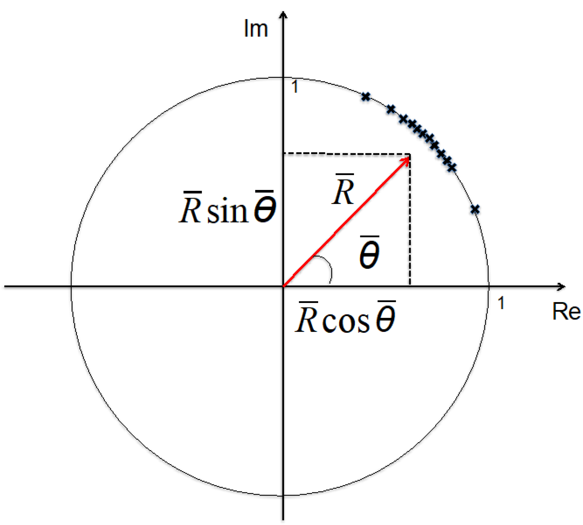
with ρ being the sampled (measured) weighted mean resultant length of the circular data , which represents the amplitude of the following complex term:
where:
Taking into account Equation (10), see also Figure 1, it is straightforward to prove (see Mardia’s book [29] for additional details) that:
Accordingly, Equation (8) can be conveniently re-written as follows:
It is worthwhile to note that the minimization of the circular variance of the random vector Θ leads to the minimal dispersion of the directional data Θ with respect to the (weighted) mean direction has also been proven.
In this research, one of the main goals is to evaluate the statistical characteristics of the directional phase residuals after the non-linear optimization in Equations (4) and (12).
The first issue is the statistical description of the (weighted) resultant length and the (weighted) mean direction . For the sake of simplicity, let us initially assume that the used weights are non-random terms (even though a generalization to the case of random independent variables leads to the same global results), and calculate the statistical average and the standard deviation of and . Let us start by considering the first statistical moments of [29]:
It is realistic to assume that, after the application of the non-linear optimization procedure in (12), the random residual phase terms can be seen as independent and identically distributed (i.i.d) random variables. In the literature, the more important families of distribution for data on a circle (i.e., directional data) are the uniform, cardiod, wrapped normal, wrapped Cauchy and von Mises distributions [29,36,37]. From statistical inference, perhaps the most useful distributions on the circle are the von Mises distributions [38]. Accordingly, in this research paper, I assume the directional data have a von Mises distribution. This assumption might be tested by considering the statistical tests provided in Reference [29]. The von Mises distribution has the following probability density function (pdf) [38]:
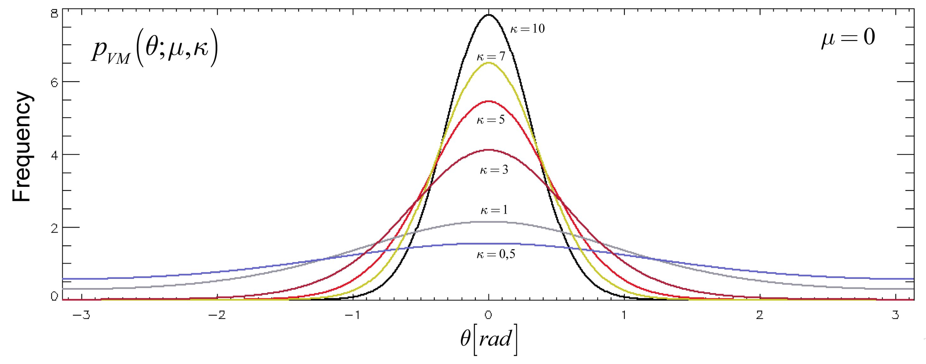
where is the modified Bessel function of the first kind and order zero, see [39]. The parameter is the mean direction and is the concentration parameter. The distribution is unimodal and symmetrical about the direction . For very small values of the concentration parameter , the von Mises distribution approximates a uniform distribution whereas, for larger values of the concentration parameter, it tends to become more concentrated at the point , as shown in Figure 2.
By assuming that is a vector of i.i.d random variables with a von Mises distribution with concentration parameter , the average expectation of the resultant weighted length is as follows:
Noteworthy, the expected (weighted) mean resultant length does not depend on the used weights. This result could seem quite counter-intuitive; however, it proves that, as long as the population is large enough (i.e., in this case, the number of interferograms ), the expected (weighted) circular variance, see also [26], is the same as the conventional circular variance (with no weights). Conversely, as clarified in the following, the statistics of the reconstructed phase components strictly depend on the used weights.
A suitable expansion of the function in (15) is as follows [29]:
As evident, depending on the (measured) value of the resultant mean length , the distribution of the phase is more or less concentrated about its mean direction . In particular, large values of correspond to more concentrated distributions of the phase residuals about their mean (weighted) direction.
Note also that as , a Von Mises distribution approximates a wrapped normal (WN) distribution. More precisely:
Specifically, the wrapped normal distribution is obtained by wrapping the normal distribution , of given mean and standard deviation values and , respectively, onto the circle, where . WN distribution has the following pdf [29]:
The calculation of the standard deviation of the (weighted) resultant length is now in order. It is straightforward to demonstrate that, at variance with the expected value, it rigorously depends on the used weights. In fact:
where and represent the mean and root mean square (RMS) values of the used weights. For von Mises distributions that are symmetrical about zero, namely , which is a reasonable assumption in our specific case, it can also be shown that:
The weights significantly modify the standard deviation of the (weighted) mean resultant length. More importantly, it is worth remarking that the standard deviation of the circular variance, see Equation (8), is the same as the standard deviation of the (weighted) resultant length. Accordingly, Equation (20) shows that the adopted estimator in (4) and (12) is an unbiased and consistent estimator of the resultant mean length of the phase population, e.g., its standard deviation tends to zero as the number of samples . Additionally, by extending the analyses provided in Reference [29] to the (weighted) circular variance estimator in Equation (4) and (12), it can also be proven that the estimator of the (weighted) mean resultant length is also an efficient estimator. Moreover, for a von Mises distribution, the maximum likelihood estimate (MLE) of the concentration parameter κ is also carried out as the solution of the following equation:
Solutions of Equation (21) are listed for different ranges of values of the (measured) mean resultant length ρ of the population. In particular, for ρ ≥ 0.85, the following relation holds:
Thus, leading one to the possibility of having an MLE estimate of the concentration parameter of the distribution from the measured (optimal) value of the circular variance (see Equations (9) and (12) again).
3.2. Statistical Characterization of the E-MTInSAR Phase Estimator
At this stage, the statistical characterization of the (weighted) mean direction estimator is in order. By the central limit theorem [40], it can be shown that the joint distribution of and is asymptotically normal, and the joint distribution of and is asymptotically bivariate.
By extending the work of Reference [29] (and references therein), the following relations are valid for von Mises distributions that are symmetrical about zero (e.g., , as it is expected in our case):
Therefore, the (weighted) mean resultant length and mean direction are asymptotically uncorrelated. By using the MLE value of the concentration parameter , see Reference (22), and after simple mathematical manipulations, it can be demonstrated that the variances of and are expressed as follows:
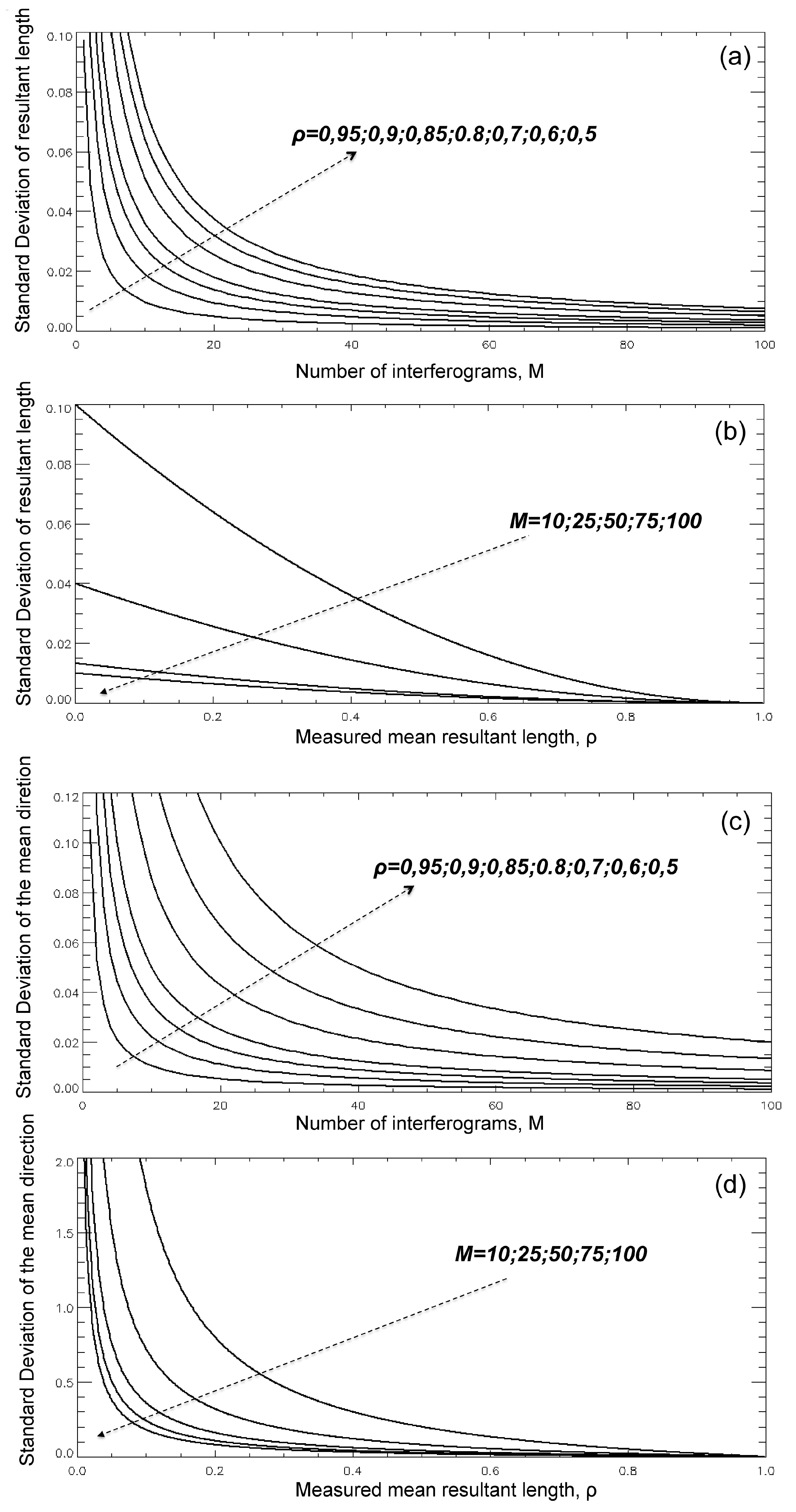
The derivation of Equation (24) is based on the general assumption that the phase is distributed with a von Mises pdf and using Equations (16) and (23) approximated to the first order. Figure 3 plots the variance of the (weighted) mean resultant length and mean direction of the random phase signal for different values of the number of interferograms and the measured value of . Equation (24) shows that the variance of the (weighted) mean resultant length and (weighted) mean direction can be calculated by the knowledge of the measured (weighted) circular variance value . An alternative derivation, which takes into account the actual characteristic of the random vector , representing the phase residuals between the original (unfiltered) and the reconstructed (filtered) interferograms, is also provided.
Starting from Equation (12), and using error source propagation rules [41], the standard deviation of the circular variance estimator of Equation (12) can be calculated as follows:
where and are the standard deviation values of the original interferograms and the optimal acquisition phases, respectively, as well as and are the corresponding phase co-variance terms. The (weighted) circular variance depends on the phases of the original interferograms as well as on the reconstructed (unknown) phases of the acquisition dates. It is worth remarking that the non-linear optimization problem in Equation (12) searches for the minimal value of the circular variance; accordingly, the estimated phase values related to every SAR acquisition correspond to a stationary point onto the N-dimensional space of every possible solution, and, as a consequence, .
Accordingly, Equation (25) simplifies as:
As said, the interferograms are computed after the application of two independent steps: the spatial multi-looking and a (potential) preliminary (single-channel) noise filtering step, performed on every single interferogram (for instance the procedure presented in References [14,19]). Although the originally computed interferograms have a given grade of dependence, since they are obtained by the same sequence of SAR data, here I can assume, for the sake of simplicity, that the interferometric phases are uncorrelated. This simplified assumption is widely adopted in the literature, even though very few InSAR studies have addressed the problem of the correlation among a group of InSAR interferograms that are computed from the same set of SAR data [42]. Accordingly, for statistical inference, I assume that the original interferograms are independent, uncorrelated and with proper standard deviation values. From the literature, it is known that if is the number of independent looks used during the spatial multi-look operation, and under proper hypotheses on the phase distribution, the standard deviation of the original multi-look interferograms is expressed as follows [12,13]:
where the terms synthetically account for the effects of the potentially used, pre-processing spatial noise-filtered approach, and are the spatial coherence values of the original interferograms, calculated in correspondence to the radar pixel under investigation. Besides, represents the number of equivalent looks employed during the multi-looking operation. Moreover, spatial coherence values can be approximated with the estimates provided by Equation (6), used as weights of the solved non-linear optimization problem. Hence, by assuming, in the first instance, that phases are uncorrelated and independent, the co-variance phase terms in Equation (26) vanish, and the following simplified relation holds:
The calculation of the term is now in order. Starting from Equation 12, after little mathematical manipulations, it is straightforward to demonstrate that:
In the stationary phase condition, i.e., by referring to the optimal circular data retrieved after the solution of the non-linear optimization problem in Equation (4), it is reasonable to approximate the sin functions in Equation (29) with their argument; thus, the following relation is obtained:
and by substitution of Equation (30) into Equation (28), the standard deviation of the phase estimator used within the E-MTInSAR algorithm is finally derived:
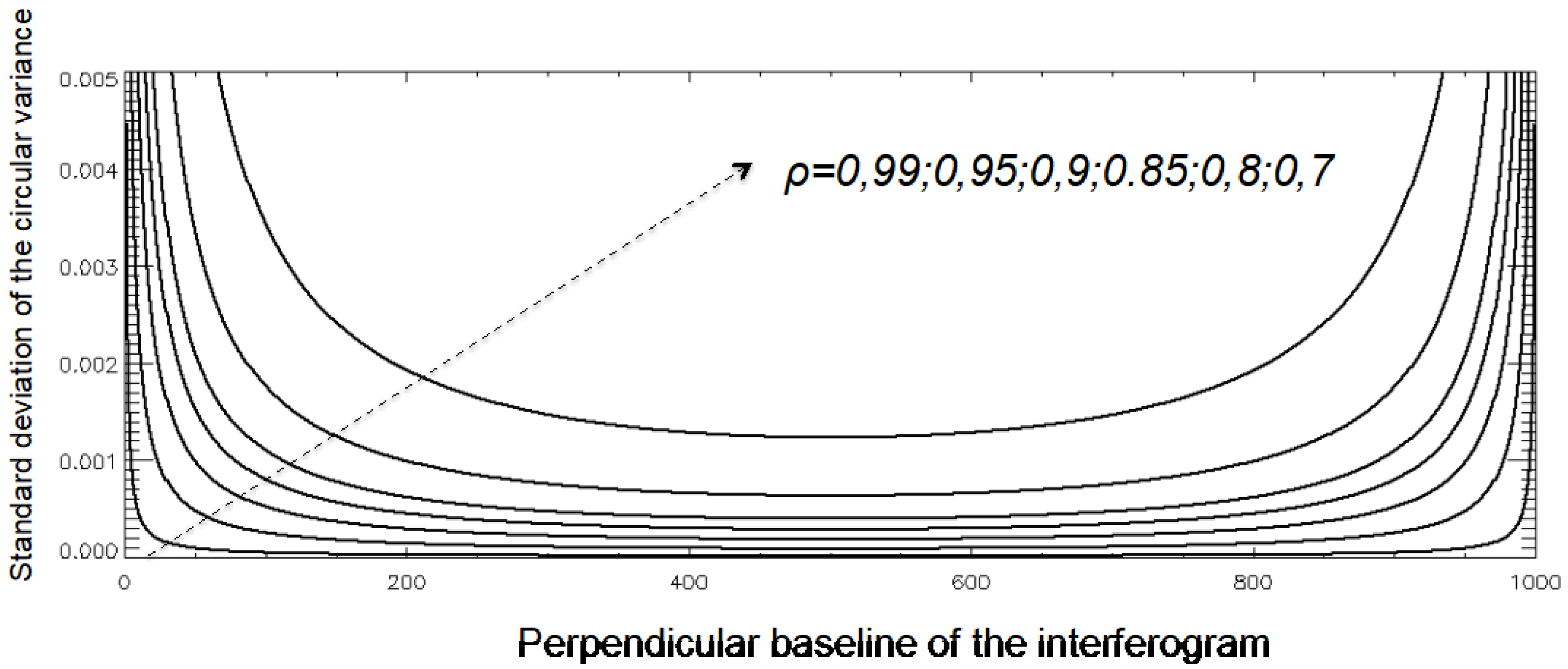
where is the average value of and is the root mean square value of the (estimated) coherence. If the resultant mean length calculated over the optimal phase estimates (i.e., on the circular data resulting from the optimization procedure) is high, we can assume the phase is distributed as a wrapped normal (WN), and we can calculate the standard deviation of the residual phase as, see Equation (18), . However, if we take into account, for the sake of simplicity, only the noise decorrelation artifacts due to the perpendicular baseline of the considered interferograms (i.e., the so-called spatial decorrelation), we also know that spatial coherence decreases as the perpendicular baseline of the interferograms, namely , increases [13]:
where is the critical baseline. Therefore, the standard deviation of the circular variation strictly depends on the perpendicular baseline values of the InSAR interferograms used within the entire non-linear optimization procedure. This result is one of the main outcomes of this research paper. The selection of more coherent interferograms has a role in the robustness of the used phase estimator. To infer the role of the perpendicular baselines, in this research, I have assumed that the perpendicular baselines of the interferograms are distributed with an exponential pdf. The experimental results carried out on real SAR data set (see Section 4) has demonstrated the suitability of this assumption. Under this hypothesis, the InSAR perpendicular baselines have the following pdf [42]:
where is the parameter of the exponential distribution [40]. The average and the root mean square values of the absolute perpendicular baseline of the interferograms are and , respectively. By considering Equation (32), then, it is easy to calculate: and . By substitution in Equation (31):
Figure 4 plots the standard deviation of versus the values of the average perpendicular baseline for different values of . In particular, I have assumed a critical baseline of 1000 m, a number of independent looks equal to L=30 and I considered M=1128 (see Section 4) and .
As evident, as the average perpendicular baseline λ approaches the critical baseline δb⊥c the standard deviation of the used estimator tends to diverge, as expected.
3.3. Theoretic Performance of the E-MTInSAR Noise Filtering Procedure
In this Subsection, I would like to give some introductory insights into the quality of the reconstructed interferograms. The obtained outcomes can be generally extended in other research fields, even very far from the one that is the subject of this research, where circular data (e.g., see [43,44,45]) are used and the estimator of Equation (4) is employed. Of course, additional experiments and further studies are needed to have a closed-form solution for the problem of the statistical characterization of the retrievable noise-filtered interferograms and the relevant DInSAR deformation products: This is a matter for future investigations.
First of all, I would like to remark that the measured optimal mean resultant length, namely , also gives an indirect estimate of the standard deviation of the residual phase, which was suitably assumed as independent and identically distributed. In particular, as earlier demonstrated: var[Θ] ≅ −2lnρ. However, the residual phases take into account both the original and the reconstructed interferograms. Accordingly, as a first approximation, if we initially assume that original and reconstructed interferograms are mutually independent, it can be argued that [42]:
However, the original interferograms are not identically distributed and, as a consequence, the same happens for the reconstructed interferograms. In particular:
Under the hypothesis of independence, it is clear that the interferograms that were formerly with low spatial coherence and large standard deviations correspond to reconstructed interferograms with small standard deviations and higher coherence values, as also experimentally demonstrated in Reference [26], and further corroborated by the experimental results shown in Section 4. Of course, the hypothesis on the independence between the original and the reconstructed interferograms should be relaxed assuming there is a specific correlation between them (see the theory on InSAR noise models addressed in Reference [42], for instance). More precisely, if we assume, for the sake of simplicity, that the original and reconstructed interferograms are jointly Gaussian with the correlation coefficient η, we can then state that:
and the following relation holds:
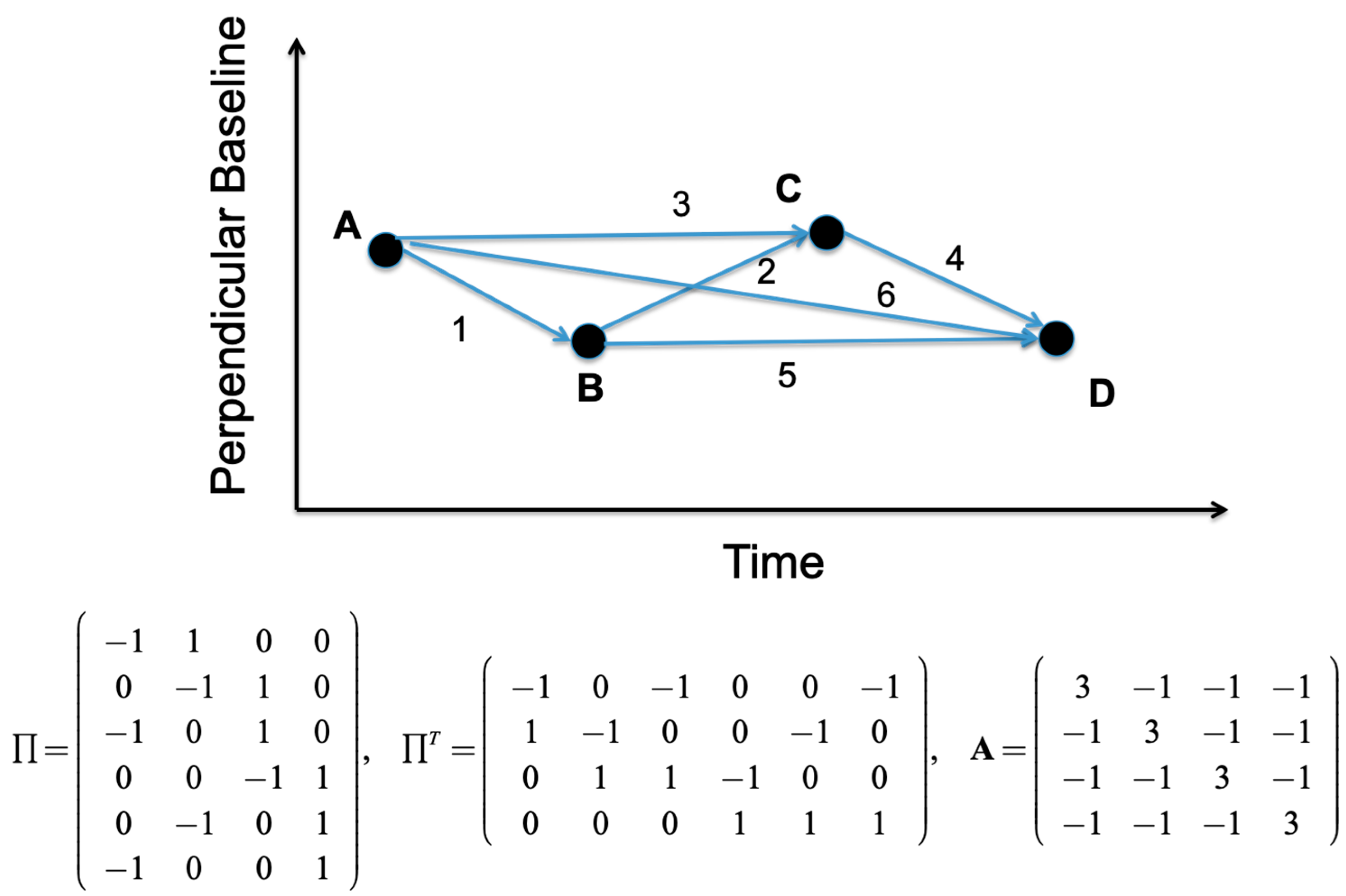
A more reliable estimate of the statistics of the reconstructed interferograms would require the knowledge of the incidence matrix ∏ of the oriented graph G representing the InSAR data distribution, which specifies the edge-node connectivity relations among the network of interferograms into the temporal/perpendicular baseline plane. Therein, the nodes of the graph identify the used SAR data and the edges the selected interferometric SAR data pairs. As an example, see the picture depicted in Figure 5, where a possible distribution of four nodes and six edges is simulated.
To infer the standard deviation of the reconstructed interferograms, the minimization of the circular variance in Equation (12) represents, again, the starting point.
As said, the optimal phase estimates related to the available SAR acquisitions are those that minimize the following mathematical operator:
In correspondence to the stationary phase point, the following relations hold:
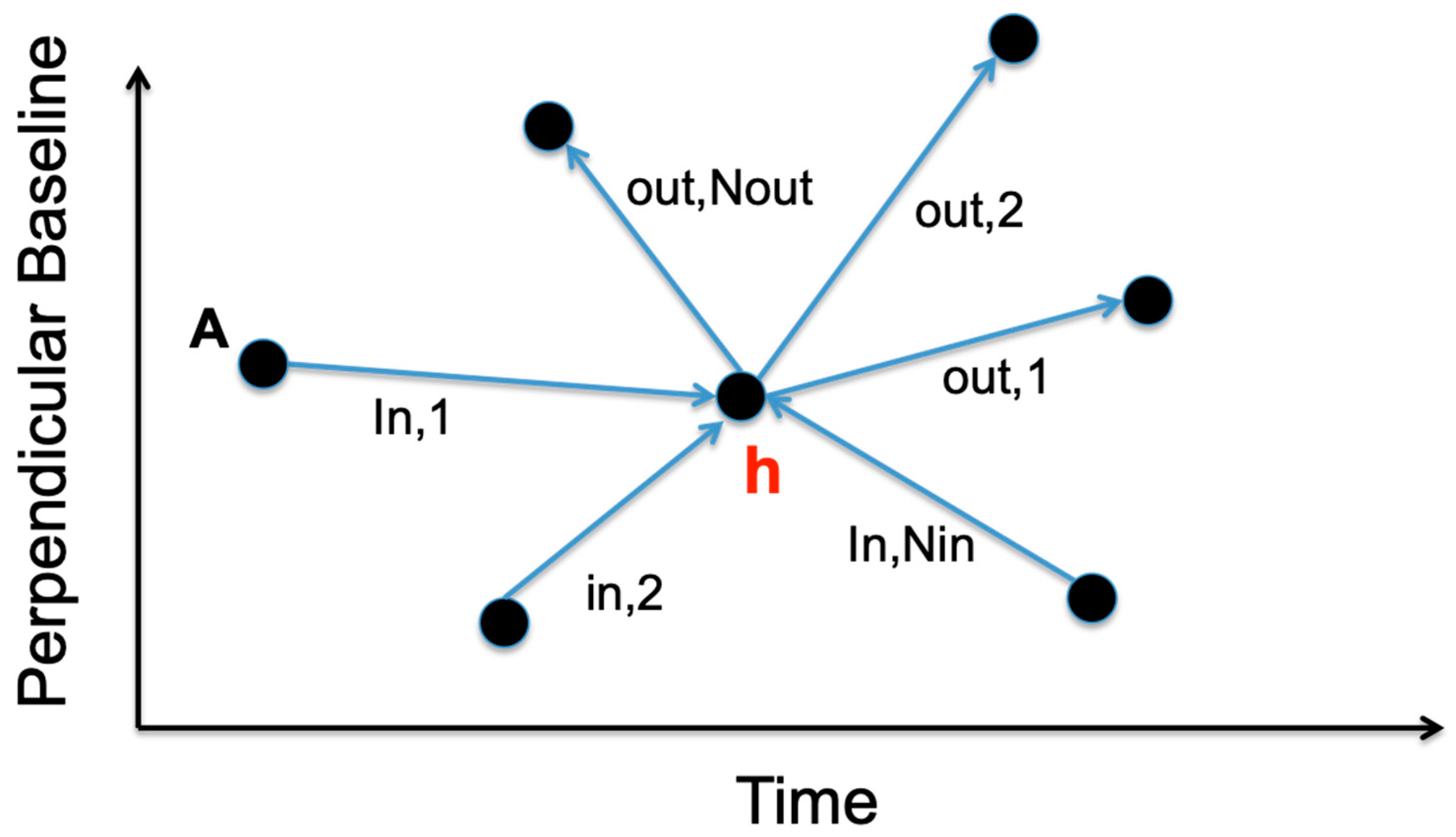
The derivative terms that are present in Equation (40) can assume values –1,0,1 depending on the fact that the h-node of the oriented graph G, see for instance the example shown in Figure 6, is involved in the i-th InSAR data pair (an edge of the graph G). In particular:
If we indicate with the number of edges that exit from the node h and with the number of edges that enter the node h, it is pretty easy to demonstrate that condition (40) is equivalent to:
Equation (42) can also be re-organized as follows:
Using matrix formalism, Equation (43) can simply be written as:
By inspecting Equation (43) and using discrete calculus principles and graph theory [46], it can be easily shown that the matrixes and can be expressed as follows:
where is the vector (Mx1) of the weights used during the optimization procedure, and the symbol∘ stands for the Hadamard product. Figure 6 shows the expression of A and B matrices for the simplified graph depicted in Figure 6. It is worth noting that if the weights are all unitary, the matrix represents the discrete Laplacian matrix [46] of the graph G; thus . The matrix has several interesting properties and is mostly used in the research field of spectral clustering [46,47]. Here, I will only mention the properties that are significant for the present research work.
The graph Laplacian matrix of a graph is defined as:
where and are the degree matrix and the adjacency matrix of the network, respectively, see [46] for details. More importantly, the matrix is: (i) Symmetric and positive semi-definite, (ii) its smallest eigenvalues is zero, and the corresponding eigenvector is the constant one vector; (iii) it has all real-valued eigenvalues. Because at least one of the eigenvalues is equal to zero, the Laplacian matrix is not invertible. However, a generalized inverse is defined using the following matrix decomposition:
where is the matrix containing all eigenvectors as columns and Λ+ is the diagonal matrix with the eigenvalues on its diagonal. Interested readers can find further details on the inverse of the Laplacian graph matrix in [47]. Another example, for a simple triangular oriented grid, is shown in Figure 7. I would also like to point out that, in the simplified case that all the weights are unitary, the following relation holds:
where the properties of the wrapping operator have been used. Indeed, the relation in Equation (44) involves (wrapped) phase terms but matrix multiplication can be only performed on absolute (unwrapped) phase quantities. However, this does not represent a severe drawback, at least when the weights are unitary, because wrapped and unwrapped phases differ by multiple-integer matrixes of . Accordingly, by using Equation (44), the expression (48) is valid.
Analysis of Equation (48) evidences another essential result of this research paper: When the phase noise vector term is not present, i.e., when the original interferograms are fully time-consistent, the reconstructed and the original interferograms are necessarily the same. This outcome is not surprising, and it demonstrates that the condition expressed by Equation (3) is required for the application of the developed noise-filtering method.
Generally speaking, the condition (see Equation (48)):
means that, under the hypothesis that original interferograms are uncorrelated, the (wrapped) discrete divergence of the reconstructed interferograms, namely , equals the (wrapped) divergence of the original interferograms, namely .
Equation (45) and the property (49) of the reconstructed interferograms may be exploited to calculate the covariance matrix of the reconstructed interferograms. In particular, for the sake of simplicity, let us refer to the (unwrapped) quantities. In this case, assuming that all weights are unitary, the covariance matrix of the optimal phase vector related to the SAR acquisition is related to the covariance matrix of the original interferograms as expressed below:
Finally, if we assume that original interferograms were all uncorrelated, independent and identically distributed with standard deviation , the co-variance matrix of the reconstructed phases related to each SAR acquisition, see Equation (50), is as follows:
The outcome expressed by Equations (50) and (51) is significant, even it is not definitive. This research paper represents a step forward to Reference [26]. Additional efforts are required to extend the result of Equation (51) in a broader context, with the aim to identify how to select and use the original interferograms to maximize the performance of the E-MTInSAR noise-filtering technique. In this framework, the role of the weights in Equation (45) has to be taken into account for future analyses.
4. Experimental Results
In this Section, I present the experiments performed on real data to address the theoretical issues discussed in the previous sections.
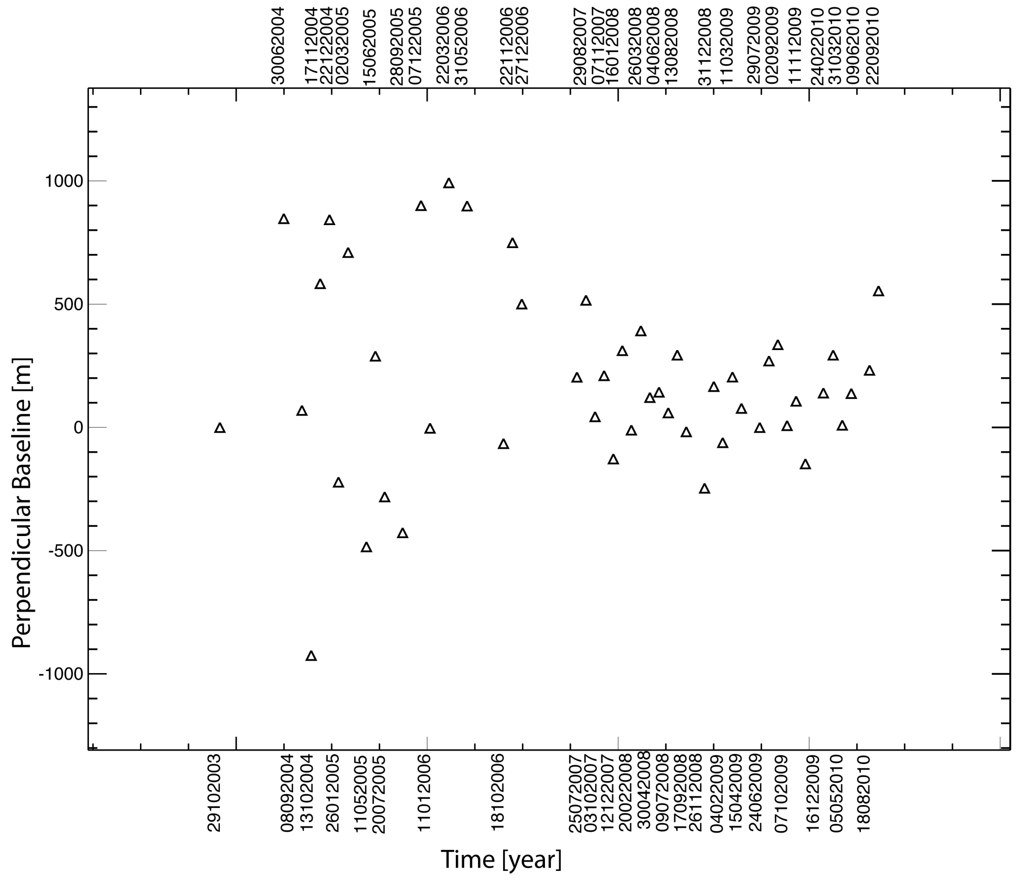
This study benefits from the availability of a sequence of SAR images acquired over a portion of the South California area by the ASAR sensor onboard the ENVISAT satellite of ESA. In particular, the SAR dataset is composed of 48 images (ascending passes, Track 120, VV polarization) collected from October 29, 2003, to September 22, 2010. SAR data were co-registered with respect to the reference SAR image acquired on October 3, 2007, which was taken as reference. The amplitude of a sample image of the case-study area is shown in Figure 8. By considering as reference the selected SAR master image, the perpendicular baseline of every SAR image has also been calculated. The distribution of the available SAR images in the time/perpendicular baseline domain is depicted in Figure 9. The experiments were initially performed by considering the entire set of M = 1128 differential SAR interferograms, without imposing any constraints on the temporal and perpendicular baseline of the used DInSAR data pairs. As discussed in Section 3, the distribution of the perpendicular baselines of the identified group of interferograms is inferred to be distributed with an exponential probability density function.
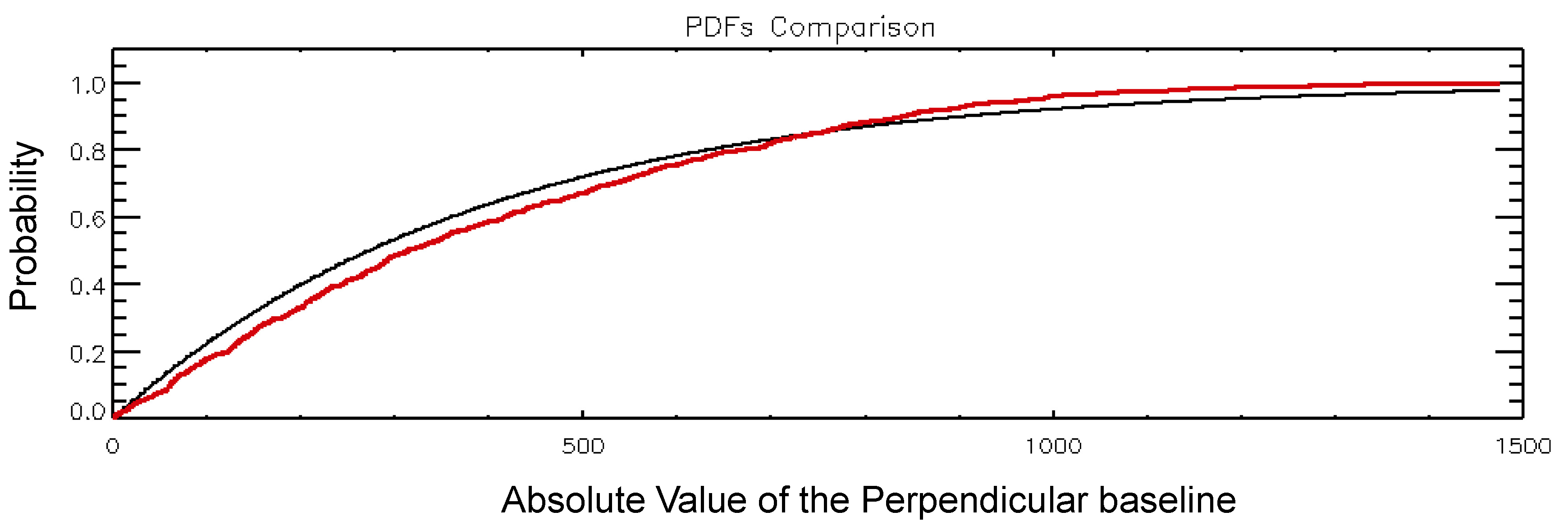
Even though a robust analysis of the statistical distribution of the InSAR baseline SAR data pair would require the availability of several SAR datasets collected by the same (or different) SAR systems, I initially focused on the available SAR distribution, and I tested the absolute value of the InSAR perpendicular baselines has an exponential pdf, see Equation (33). To this aim, the average value of the distribution was first calculated, namely a value of about 393.241 m was found. Accordingly, the cumulative distributive function of the reference exponential distribution was derived and compared to the empirical distribution function, see Figure 10. Then, the Kolmogorov Smirnov (K–S) test [43] was applied. The objective was to test the hypothesis H0 against the hypothesis. K–S is a non-parametric test that relies on the estimate of the distance between the empirical and the cumulative theory distributions of a known distribution. In particular, the following quantity is calculated:
The test accepts the hypothesis H0 with a given significance level. In the case of the South California case-study test-site, the K–S test was accepted with a significance level of 0.01.
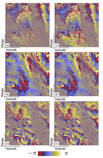
Once identified, the M differential interferograms were generated. To this purpose, precise satellite information and a three-arc digital elevation model (DEM) of the area were used to remove the topographic phase components. Computed interferograms were independently multi-looked (20 azimuth and 4 range looks, respectively) and also pre-filtered using the approach described in [14]. The E-MTInSAR noise-filtering method was initially applied to the whole set of interferograms. As extensively discussed in Reference [26], it was expected that some interferograms were significantly depurated by noise artifacts, as indirectly testified by the increased level of coherence. On the contrary, a few of the very good interferograms were expected to be degraded by the filter. Four interferograms, characterized by different values of the perpendicular baseline, have been selected and shown in Figure 11, before and after the application of the noise-filtering algorithm.
It is evident that the interferograms with moderate-to-low coherence were significantly improved, at the partial expenses of the quality of the original, very high coherent interferograms. As said, a post-processing step is applied in the improved EMCF-SBAS processing chain, but here the focus has exclusively been on showing only the interferograms reconstructed by the core E-MTInSAR noise-filtering procedure.
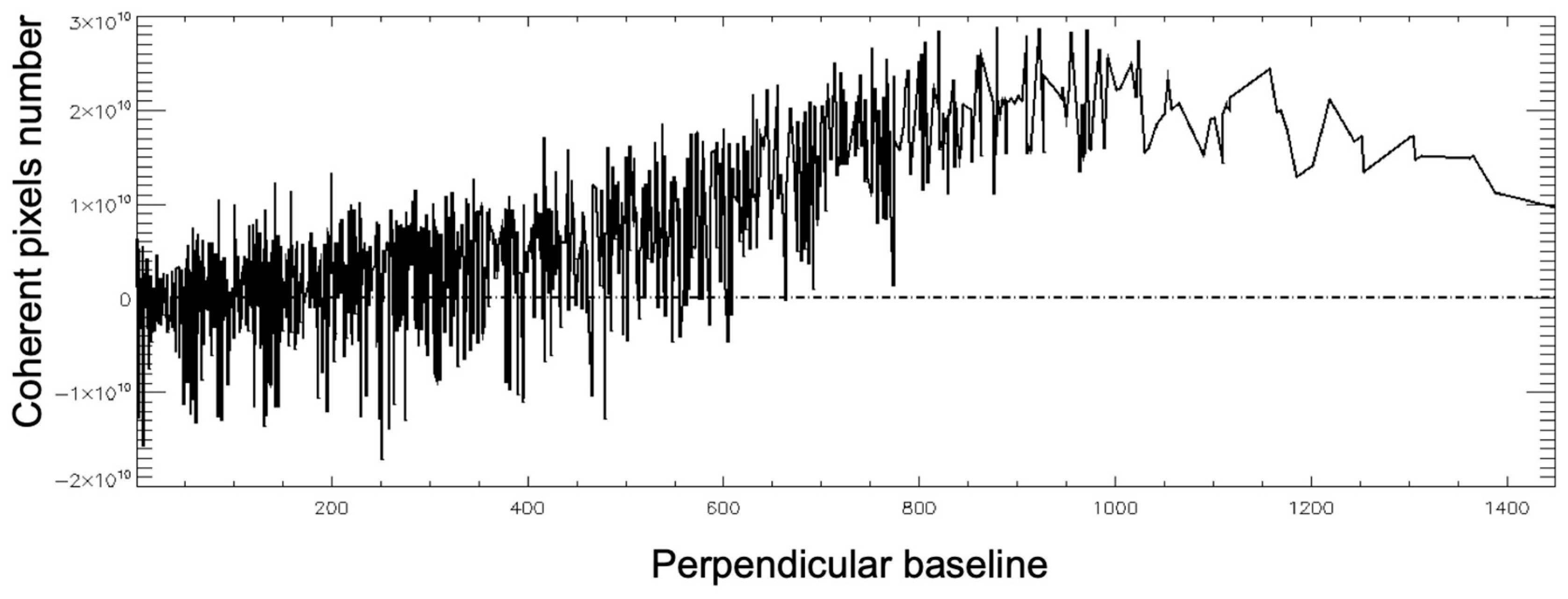
In Figure 12 the number of coherent pixels (a threshold coherence of 0.5 has been applied) as a function of the perpendicular baseline of the considered interferograms is depicted. In this experiment, all the InSAR data pairs were used for the inversion. I would like to remark that experimental results are in general agreement with the theory addressed in Section 4 and with the experiments presented in previous works [26,48]. Similarly, to what was provided initially in Reference [26], I also repeated the same test by progressively discarding from the entire group of SAR interferograms those exhibiting perpendicular baseline values larger than a given threshold. In particular, I selected five groups of SB interferograms by using thresholds on the interferometric perpendicular baseline values of 300 m, 400 m, 500 m, 600 m, and 800 m, respectively. As a reference for the calculation of the general performance of the algorithm, I also assumed the set of SB interferograms selected imposing a maximum perpendicular baseline value of 300 m.
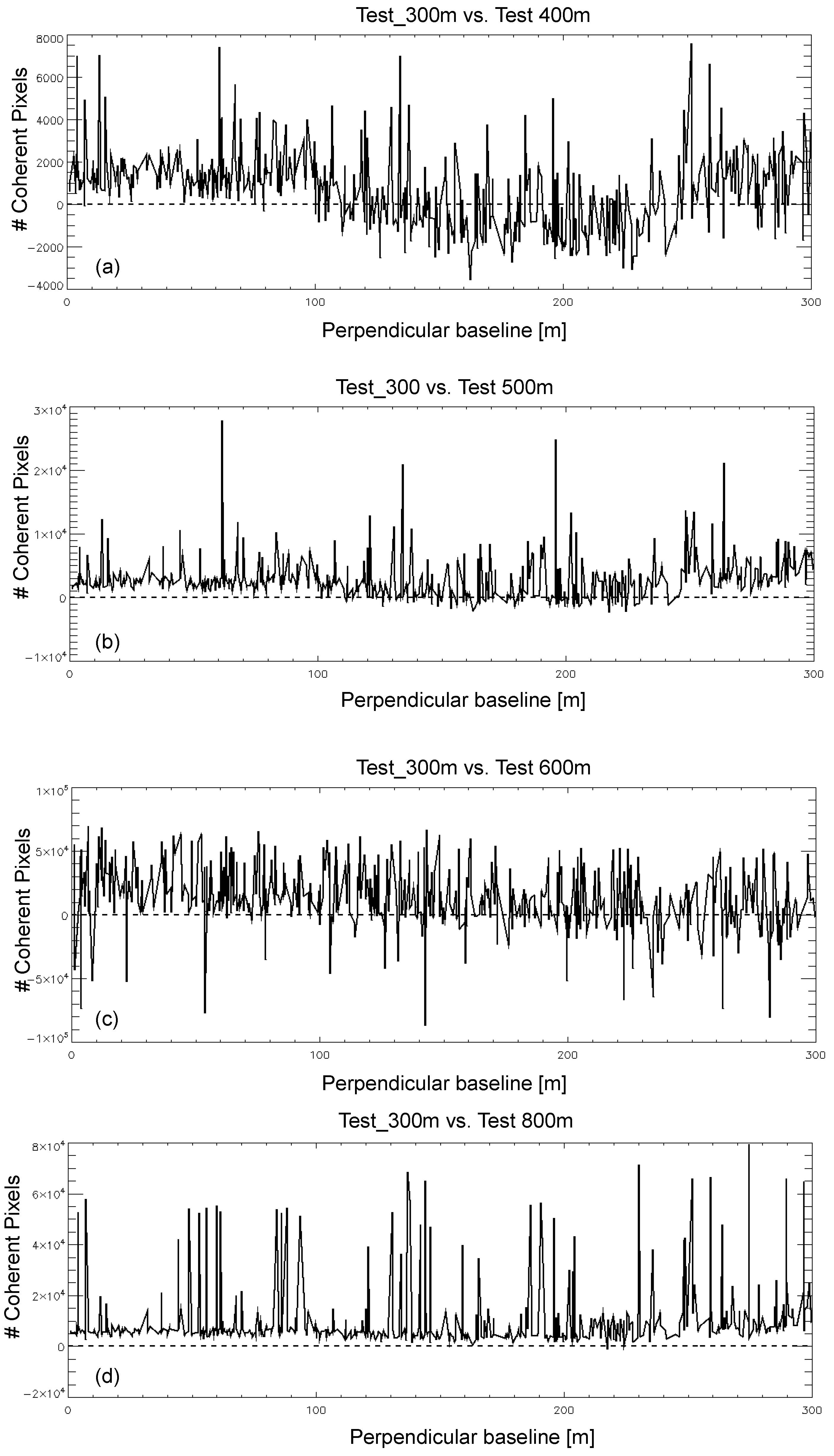
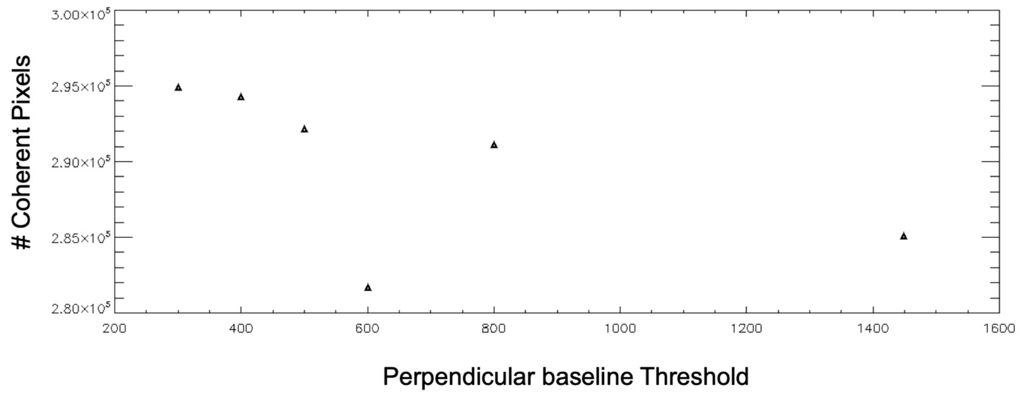
Figure 13 shows the comparison between the numbers of coherent pixels identified in the different tests. In particular, for each run of the algorithm with different InSAR graphs, the difference between the numbers of coherent pixels detected at the given run, and those obtained by considering the entire InSAR network graph composed by 1128 SAR data pairs was computed. As evident, as the baseline threshold decreases and sets of SB interferograms are selected the number of coherent pixels increases. This testifies that the standard deviation of the original interferograms has a role in the optimization procedure, as indicated by the sample covariance matrix relationship expressed by Equations (50) and (51). Finally, Figure 14 plots the number of the whole coherent pixels of the set of SB interferograms corresponding to the test carried out by using a perpendicular baseline threshold of 300 m (which has been used as a reference).
Further extended theory investigations and experimental analyses are, however, required to have direct confirmation of the validity of the theoretical outcomes of this research study. In particular, some new InSAR noise models have to be developed to incorporate these new kinds of multi-temporal noise-filtered interferograms.
As originally provided in Reference [26], I repeated the same experiment by progressively discarding from the entire group of SAR interferograms, those exhibiting perpendicular baseline values larger than a given threshold. In particular, I selected five groups of SB interferograms with a threshold on the perpendicular baseline of 300 m, 400 m, 500 m, 600 m, 800 m and without considering any constraints, respectively.
Figure 15 shows a comparison between the average spatial coherence of the original (unfiltered) and the reconstructed (filtered) sequence of multi-looked interferograms for the selected case-study area. Globally, the average coherence increased about 5%. This paper is, at most, focused on the presentation of the statistics fundaments of the core E-MTInSAR algorithm, instead of the general performance of the improved EMCF-SBAS processing chain. Interested readers can find additional details on the improved EMCF-SBAS InSAR toolbox, as well as an overview of some experimental results in the literature, see for instance [48,49,50].
5. Discussion
This research paper addresses the theoretical basis of the E-MTInSAR noise-filtering algorithm, relying on the use of directional statics [29]. Even though the algorithm is complemented within the improved EMCF-SBAS processing chain, here, the interest is more focused on the performance of the core non-linear optimization procedure of Equation (4) and the retrieval of the reconstructed noise-filtered multi-look interferograms. As already stated in a previous publication [26], the distinctive characteristic of the adopted noise-filtering technique is the use of the temporal relationships among a time-redundant set of “conventional” differential multi-looked interferograms. Previous multi-temporal noise-filtered solutions, such as SqueeSAR [11], CaeSAR [27] and other alternative methods [24,25] have already addressed this problem. They rely on the validity of the distributed scattering hypothesis under which the probability density function (pdf) of the complex-valued SAR image may be regarded as being a zero-mean multivariate circular normal distribution, and appropriate analyses are required to identify DS targets for which these hypotheses are valid. Conversely, the adopted noise-filtered method does not need any specific assumption on the statistical distribution of the multi-looked phases of DS targets, which are challenging to be inferred, especially when additional pre-processing, single-channel noise-filtering steps (e.g., the Goldstein’s filter [14]) are also preliminarily applied to the generated interferograms. Nonetheless, the identification of statistically homogenous pixels (SHPs) and the implementation of a suitable adaptive multi-looking step, as suggested in Reference [30], might be considered as a further evolution of the E-MTInSAR algorithm. This research study has demonstrated from a mathematical and statistical perspective that: (i) The phase estimator in Equation (12) is consistent and the measured (optimal) weighted circular variance value gives a direct figure of the standard deviation of the circular variance estimator in Equation (12); (ii) the standard deviation of the circular variance estimator adopted in Equation (12) critically depends not only on the number of used interferograms, namely M, but also on the absolute value of the perpendicular baseline of these interferograms, in particular, as the average absolute perpendicular baseline approaches the critical baseline the estimator diverges; (iii) the actual standard deviation of the reconstructed, noise-filtered interferograms strictly depends on the phase stability of the original interferograms, the overall graph network of used interferograms, see Equations (50) and (51), and the presence of the time-inconsistencies, namely the signal D, in the original interferograms. Equation (51) opens up the possibility to evaluate the global performance of the algorithm in terms of phase stability of the reconstructed interferograms. Potentially, it can be used to assess, from a theoretical point of view, the performance of the InSAR products, e.g., displacement time-series and mean displacement velocity maps, of the multi-temporal interferometric processing chain, such as the improved EMCF-SBAS, where the E-MTInSAR noise-filtering approach is implemented. This requires, however, further efforts because it is needed to deeply study the statistical dependence of sequences of time-redundant sets of differential SAR interferograms. Only a few studies are available in the literature on this very challenging issue, which would allow determining the error budget of the above-mentioned InSAR products, on a pixel-by-pixel basis, by merely knowing the Laplacian matrix of the InSAR graph representing the network of used interferograms. The outcomes of this research are also suitable to be extended in other research contexts where multi-temporal/multi-dimensional circular data [43,44,45] are used.
6. Conclusions and Future Perspectives
This research provided new insights into the theory at the base of the enhanced multi-temporal noise-filtering method, which was initially proposed as a further improvement of the EMCF-based SBAS processing chain [26]. This research permitted studying the statistical behavior of the adopted estimator for the unknown phases related to every SAR acquisitions. Furthermore, the theoretical relationship between the covariance matrix of the original and the reconstructed noise-filtered interferograms has been derived. The validity of these equations has been proven by referring to the fundamentals of directional statistics [29] and discrete calculus [32]. In the light of the application of the E-MTInSAR technique in a real scenario, several questions are still open and require answers. Of great significance, in particular, is the evaluation, from a theory perspectives, of the optimal perpendicular baseline threshold used for selecting the group of SB interferograms employed for surface deformation maps retrieval. Experimentally, using reduced, time-redundant sets of SB interferograms is more convenient and globally guarantees better performances. The identification of such optimal thresholds requires, as outlined in the previous section, the application of graph theory selection-based strategies. These approaches for the identification of the most suitable graph of InSAR interferograms might also be complemented with the interferogram selection algorithm proposed in [26]. Furthermore, one of the next steps of this research is to evaluate the general performance of the improved EMCF-SBAS processing tool [26] and, in particular, to get an estimate of the precision and accuracy of the DInSAR products, i.e., deformation time-series and ground mean deformation velocity maps.
Author Contributions
A.P. is the principal investigator of this research study.
Funding
This research received no external funding.
Acknowledgments
I acknowledge the I-AMICA project of structural improvement financed under the National Operational Programme (PON) for “Research and Competitiveness 2007–2013”, co-funded with the European Regional Development Fund (ERDF) and National Resources. URBAN-GEO BIG DATA, a Project of National Interest (PRIN) funded by the Italian Ministry of Education, University and Research (MIUR), id. 20159CNLW8, has partly funded this research study. I would also like to express my gratitude to my parents and the students of Signal Theory at the University of Basilicata, Potenza, Italy, for the valuable suggestions and help I received from all of them during the recent few years. Finally, I thank Simone Guarino, Fernando Parisi and Maria Consiglia Rasulo for the technical help and support.
Conflicts of Interest
The author declares no conflict of interest.
References
- Ferretti, A.; Prati, C.; Rocca, F. Permanent scatterers in SAR interferometry. IEEE Trans. Geosci. Remote Sens. 2001, 39, 8–20. [Google Scholar] [CrossRef]
- Kampes, B.M. Radar Interferometry: Persistent Scatterer Technique; Springer: New York, NY, USA, 2006. [Google Scholar]
- Werner, C.; Wegmuller, U.; Strozzi, T.; Wiesmann, A. Interferometric point target analysis for deformation mapping. In Proceedings of the IEEE International Geoscience and Remote Sensing Symposium, Toulouse, France, 21–25 July 2003; Volume 7, pp. 4362–4364. [Google Scholar]
- Hooper, A.; Zebker, H.; Segall, P.; Kampes, B.M. A new method for measuring deformation on volcanoes and other natural terrains using InSAR persistent scatterers. Geophys. Res. Lett. 2004, 31, L23611. [Google Scholar] [CrossRef]
- Berardino, P.; Fornaro, G.; Lanari, R.; Sansosti, E. A new algorithm for surface deformation monitoring based on small baseline differential SAR interferograms. IEEE Trans. Geosci. Remote Sens. 2004, 40, 2375–2383. [Google Scholar] [CrossRef]
- Lanari, R.; Mora, O.; Manunta, M.; Mallorquì, J.J.; Berardino, P.; Sansosti, E. A small baseline approach for investigating deformation on full resolution differential SAR interferograms. IEEE Trans. Geosci Remote Sens. 2004, 42, 1377–1386. [Google Scholar] [CrossRef]
- Mora, O.; Mallorquı, J.J.; Broquetas, A. Linear and nonlinear terrain deformation maps from a reduced set of interferometric SAR images. IEEE Trans. Geosci. Remote Sens. 2003, 41, 2243–2253. [Google Scholar] [CrossRef]
- Crosetto, M.; Crippa, B.; Biescas, E. Early detection and in-depth analysis of deformation phenomena by Radar interferometry. Eng. Geol. 2005, 79, 81–91. [Google Scholar] [CrossRef]
- Hetland, E.A.; Muse, P.; Simons, M.; Lin, Y.N.; Agram, P.S.; DiCaprio, C.J. Multiscale InSAR time series (MInTS) analysis of surface deformation. J. Geophys. Res. Solid Earth 2012, 117, B02404. [Google Scholar] [CrossRef]
- Hooper, A. A multi-temporal InSAR method incorporating both persistent scatterer and small baseline approaches. Geophys. Res. Lett. 2008, 35, L16302. [Google Scholar] [CrossRef]
- Ferretti, A.; Fumagalli, A.; Novali, F.; Prati, C.; Rocca, V.; Rucci, A. A New Algorithm for Processing Interferometric Data-Stacks: SqueeSAR. IEEE Trans. Geosci. Remote Sens. 2011, 49, 3460–3470. [Google Scholar] [CrossRef]
- Zebker, H.A.; Villasenor, J. Decorrelation in interferometric radar echoes. IEEE Trans. Geosci. Remote Sens. 1992, 30, 950–959. [Google Scholar] [CrossRef]
- Bamler, R.; Hartl, P. Synthetic Aperture Radar interferometry. Inverse Probl. 1998, 14, R1–R54. [Google Scholar] [CrossRef]
- Goldstein, R.M.; Werner, C.L. Radar interferogram filtering for geophysical applications. Geophys. Res. Lett. 1998, 25, 4035–4038. [Google Scholar] [CrossRef]
- Lee, J.-S.; Papathanassiou, K.P.; Ainsworth, T.L.; Grunes, M.R.; Reigber, A. A New Technique for Noise Filtering of SAR Interferometric Phase Images. IEEE Trans. Geosci. Remote Sens. 1998, 36, 1456–1465. [Google Scholar]
- Just, D.; Bamler, R. Phase statistics of interferograms with applications to synthetic aperture radar. Appl. Opt. 1994, 33, 4361–4368. [Google Scholar] [CrossRef] [PubMed]
- Lee, J.-S.; Hoppel, K.W.; Mango, S.A.; Miller, A.R. Intensity and Phase Statistics of Multilook Polarimetric and Interferometric SAR Imagery. IEEE Trans. Geosci. Remote Sens. 1994, 32, 1017–1028. [Google Scholar]
- López-Martínez, C.; Pottier, E. On the Extension of Multidimensional Speckle Noise Model from Single-Look to Multilook SAR Imagery. IEEE Trans. Geosci. Remote Sens. 2007, 45, 305–320. [Google Scholar] [CrossRef]
- Baran, I.; Stewart, M.P.; Kampes, B.M.; Perski, Z.; Lilly, P. A Modification to the Goldstein Radar Interferogram Filter. IEEE Geosci. Remote Sens. Lett. 2003, 41, 2114–2118. [Google Scholar] [CrossRef]
- Wang, Q.; Huang, H.; Yu, A.; Dong, Z. An Efficient and Adaptive Approach for Noise Filtering of SAR Interferometric Phase Images. IEEE Geosci. Remote Sens. Lett. 2011, 8, 1140–1144. [Google Scholar] [CrossRef]
- Fu, S.; Long, X.; Yang, X.; Yu, Q. Directionally Adaptive Filter for Synthetic Aperture Radar Interferometric Phase Images. IEEE Geosci. Remote Sens. Lett. 2013, 51, 552–559. [Google Scholar] [CrossRef]
- Lee, J.S.; Pottier, E. Polarimetric Radar Imaging: From Basics to Applications; CRC Press: Boca Raton, FL, USA, 2009. [Google Scholar]
- Deledalle, C.-A.; Denis, L.; Tupin, F. NL-InSAR: Nonlocal Interferogram Estimation. IEEE Trans. Geosci. Remote Sens. 2011, 49, 1441–1452. [Google Scholar] [CrossRef]
- Parizzi, A.; Brcic, R. Adaptive InSAR stack multi-looking exploiting amplitude statistics: A comparison bbetween different techniques and practical results. IEEE Geosci. Remote Sens. Lett. 2011, 8, 441–445. [Google Scholar] [CrossRef]
- Pinel-Puyssegur, B.; Michel, R.; Avouac, J.P. Multi-link InSAR time-series: Enhancement of a wrapped interferometric database. IEEE J. Sel. Top. Appl. Earth Obs. Remote Sens. 2012, 5, 784–794. [Google Scholar] [CrossRef]
- Pepe, A.; Yang, Y.; Manzo, M.; Lanari, R. Improved EMCF-SBAS Processing Chain Based on Advanced Techniques for the Noise-Filtering and Selection of Small Baseline Multi-look DInSAR Interferograms. IEEE Trans. Geosci. Remote Sens. 2015, 53, 4394–4417. [Google Scholar] [CrossRef]
- Fornaro, G.; Verde, S.; Reale, D.; Pauciullo, A. CAESAR: An Approach Based on Covariance Matrix Decomposition to Improve Multibaseline Multitemporal Interferometric SAR Processing. IEEE Trans. Geosc. Remote Sens. 2015, 53, 2050–2065. [Google Scholar] [CrossRef]
- Pepe, A.; Lanari, R. On the Extension of the Minimum Cost Flow Algorithm for Phase Unwrapping of Multitemporal Differential SAR Interferograms. IEEE Trans. Geosci. Remote Sens. 2006, 44, 2374–2383. [Google Scholar] [CrossRef]
- Mardia, K.V.; Jupp, P.E. Directional Statistics; Wiley: New York, NY, USA, 2000. [Google Scholar]
- Pepe, A.; Mastro, P. On the use of directional statistics for the adaptive spatial multi-looking of sequences of differential SAR interferograms. In Proceedings of the 2017 IEEE International Geoscience and Remote Sensing Symposium (IGARSS), Fort Worth, TX, USA, 23–28 July 2017; pp. 3791–3794. [Google Scholar]
- Grady, L.J.; Polimeni, J. Discrete Calculus: Applied Analysis on Graphs for Computational Science; Springer: New York, NY, USA, 2010. [Google Scholar]
- Biggs, N. Algebraic Graph Theory; Cambridge University Press: Cambridge, UK, 1994. [Google Scholar]
- Torres, R.; Snoeij, P.; Geudtner, D.; Bibby, D.; Davidson, M.; Attema, E.; Potin, P.; Rommen, B.; Floury, N.; Brown, M.; et al. GMES Sentinel-1 mission. Remote Sens. Environ. 2012, 120, 9–24. [Google Scholar] [CrossRef]
- Shimada, M.; Watanabe, M.; Motooka, T.; Kankaku, Y.; Suzuki, S. Calibration and validation of the PALSAR-2. In Proceedings of the IGARSS International Geoscience and Remote Sensing Symposium 2015, Milan, Italy, 26–31 July 2015. [Google Scholar]
- Imperatore, P.; Pepe, A.; Lanari, R. Multi-Channel Phase Unwrapping: Problem Topology and Dual-Level Parallel Computational Model. IEEE Trans. Geosci. Remote Sens. 2015, 53, 5774–5793. [Google Scholar] [CrossRef]
- Downs, T.D.; Mardia, K.V. Circular regression. Biometrika 2002, 89, 683–697. [Google Scholar] [CrossRef]
- Shieh, G.S.; Johnson, R.A. Inferences based on a bivariate distribution with von Mises marginal. Ann. I. Stat. Math. 2005, 57, 789–802. [Google Scholar] [CrossRef]
- Von Mises, R. Uber die Ganzzahligkeit der Atomgewichte und verwandte Gragen. Phys. Z. 1918, 19, 490–500. [Google Scholar]
- Olver, F.W.J.; Maximon, L.C. Bessel function. In NIST Handbook of Mathematical Functions; Olver, F.W.J., Lozier, D.M., Boisvert, R.F., Clark, C.W., Eds.; Cambridge University Press: Cambridge, UK, 2010; ISBN 978-0521192255. [Google Scholar]
- Papoulis, A. Probability, Random Variables and Stochastic Processes, 3rd ed.; McGraw-Hill Education: New York, NY, USA, 1965. [Google Scholar]
- Draper, N.R.; Smith, H. Applied Regression Analysis; Wiley: Hoboken, NJ, USA, 1988. [Google Scholar]
- Agram, P.S.; Simons, M. A noise model for InSAR time-series. J. Geophys. Res. Solid Earth. 2015, 120, 2752–2771. [Google Scholar] [CrossRef]
- Watson, G.S. Orientation statistics in the earth sciences. Bull. Geol. Inst. Univ. Uppsala 1970, 2, 73–89. [Google Scholar]
- Batshelet, E. Circular Statistics in Biology; Academic Press: London, UK, 1981. [Google Scholar]
- Chang, T. Spherical regression and the statistics of tectonic plate reconstructions. Internat. Statist. Rev. 1993, 61, 299–316. [Google Scholar] [CrossRef]
- Chung, F.R.K. Spectral Graph Theory; CBMS Regional Conference Series in Mathematics, No. 92; American Mathematical Society: Providence, RI, USA, 1997. [Google Scholar]
- Gutman, I.; Xiao, W. Generalized inverse of the Laplacian matrix and some applications. Bulletin de l’Academie Serbe des Sciences at des Arts 2004, 129, 15–23. [Google Scholar] [CrossRef]
- Yang, Y.; Pepe, A.; Manzo, M.; Bonano, M.; Liang, D.N.; Lanari, R. A simple solution to mitigate noise effects in time-redundant sequences of small baseline multi-look DInSAR interferograms. Remote Sens. Lett. 2013, 4, 609–618. [Google Scholar] [CrossRef]
- Pepe, A.; Calò, F. A Review of Interferometric Synthetic Aperture RADAR (InSAR) Multi-Track Approaches for the Retrieval of Earth’s Surface Displacements. Appl. Sci. 2017, 7. [Google Scholar]
- Pepe, A. Generation of Earth’s Surface Three-Dimensional (3-D) Displacement Time-Series by Multiple-Platform SAR Data. Available online: https://www.intechopen.com/books/time-series-analysis-and-applications/generation-of-earth-s-surface-three-dimensional-3-d-displacement-time-series-by-multiple-platform-sa (accessed on 11 February 2019).
Figure 1.
Pictorial representation of a directional data. Black stars identify the relevant phases, and the red arrow represents the mean resultant vector .
Figure 1.
Pictorial representation of a directional data. Black stars identify the relevant phases, and the red arrow represents the mean resultant vector .

Figure 2.
Von Mises probability density function (pdf) for different values of the concentration parameter .
Figure 2.
Von Mises probability density function (pdf) for different values of the concentration parameter .

Figure 3.
(a,b) Plots of the standard deviation of with respect to the number of interferograms and ρ, respectively. (b,c) Same as (a,b) but for the standard deviation of .
Figure 3.
(a,b) Plots of the standard deviation of with respect to the number of interferograms and ρ, respectively. (b,c) Same as (a,b) but for the standard deviation of .

Figure 4.
Plot of the standard deviation of ν vs. the average value of the perpendicular baseline of the population SAR data distribution.
Figure 4.
Plot of the standard deviation of ν vs. the average value of the perpendicular baseline of the population SAR data distribution.

Figure 5.
A pictorial graph with four nodes and six edges.

Figure 6.
Representation of the graph connections related to the node h.

Figure 7.
A triangular-shaped graph and its corresponding discrete calculus matrices.

Figure 8.
Amplitude SAR image of the investigated area in South California.

Figure 9.
Distribution of the South California SAR data in temporal/perpendicular baseline plane.

Figure 10.
Comparison between the theoretical (black line) and the estimated cumulative distribution function (cdf) (red line) of the perpendicular baseline SAR data distributions of the South California dataset.
Figure 10.
Comparison between the theoretical (black line) and the estimated cumulative distribution function (cdf) (red line) of the perpendicular baseline SAR data distributions of the South California dataset.

Figure 11.
Comparison between the original (left) and the reconstructed interferograms of the South California case-study area. The relevant SAR data pairs are: (a)–(a’) 22 December 2004–9 June 2010 (perpendicular baseline of 696 m); (b)–(b’) 29 August 2007–26 March 2008 (perpendicular baseline of 120 m); (c)–(c’) 29 August 2007–12 December 2007 (perpendicular baseline of 623 m).

Figure 12.
Plot of the numbers of coherent pixels vs. the perpendicular baseline for the reconstructed interferograms obtained using the entire set of 1128 original InSAR interferograms.
Figure 12.
Plot of the numbers of coherent pixels vs. the perpendicular baseline for the reconstructed interferograms obtained using the entire set of 1128 original InSAR interferograms.

Figure 13.
Comparison of the achieved results, in terms of numbers of coherent pixels, obtained by using reduced InSAR network. Plot (a–d) show the difference of the coherent pixels in the study area between the reference test (with a perpendicular baseline threshold of 300 m) and each of the four tests (with perpendicular baseline thresholds of 400 m, 500 m, 600 m, 800 m, respectively).

Figure 14.
Number of coherent pixels vs. the used perpendicular baseline threshold.

Figure 15.
Average spatial coherence of the study area as obtained using (left) original interferograms and (right) reconstructed interferograms. The test is obtained by applying a threshold of 300 m for the maximum absolute value of the perpendicular baseline of the interferometric SAR data pairs. Red boxes identify the area where a significant improvement of the average spatial coherence is obtained.

© 2019 by the author. Licensee MDPI, Basel, Switzerland. This article is an open access article distributed under the terms and conditions of the Creative Commons Attribution (CC BY) license (http://creativecommons.org/licenses/by/4.0/).
Share and Cite
MDPI and ACS Style
Pepe, A. Theory and Statistical Description of the Enhanced Multi-Temporal InSAR (E-MTInSAR) Noise-Filtering Algorithm. Remote Sens. 2019, 11, 363. https://0-doi-org.brum.beds.ac.uk/10.3390/rs11030363
AMA Style
Pepe A. Theory and Statistical Description of the Enhanced Multi-Temporal InSAR (E-MTInSAR) Noise-Filtering Algorithm. Remote Sensing. 2019; 11(3):363. https://0-doi-org.brum.beds.ac.uk/10.3390/rs11030363
Chicago/Turabian StylePepe, Antonio. 2019. "Theory and Statistical Description of the Enhanced Multi-Temporal InSAR (E-MTInSAR) Noise-Filtering Algorithm" Remote Sensing 11, no. 3: 363. https://0-doi-org.brum.beds.ac.uk/10.3390/rs11030363
Note that from the first issue of 2016, this journal uses article numbers instead of page numbers. See further details here.