Monitoring Drought Effects on Vegetation Productivity Using Satellite Solar-Induced Chlorophyll Fluorescence

Abstract

Around the world, the increasing drought, which is exacerbated by climate change, has significant impacts on vegetation carbon assimilation. Identifying how short-term climate anomalies influence vegetation productivity in a timely and accurate manner at the satellite scale is crucial to monitoring drought. Satellite solar-induced chlorophyll fluorescence (SIF) has recently been reported as a direct proxy of actual vegetation photosynthesis and has more advantages than traditional vegetation indices (e.g., the Normalized Difference Vegetation Index, NDVI and the Enhanced Vegetation Index, EVI) in monitoring vegetation vitality. This study aims to evaluate the feasibility of SIF in interpreting drought effects on vegetation productivity in Victoria, Australia, where heat stress and drought are often reported. Drought-induced variations in SIF and absorbed photosynthetically active radiation (APAR) estimations based on NDVI and EVI were investigated and validated against results indicated by gross primary production (GPP). We first compared drought responses of GPP and vegetation proxies (SIF and APAR) during the 2009 drought event, considering potential biome-dependency. Results showed that SIF exhibited more consistent declines with GPP losses induced by drought than did APAR estimations during the 2009 drought period in space and time, where APAR had obvious lagged responses compared with SIF, especially in evergreen broadleaf forest land. We then estimated the sensitivities of the aforementioned variables to meteorology anomalies using the ARx model, where memory effects were considered, and compared the correlations of GPP anomaly with the anomalies of vegetation proxies during a relatively long period (2007–2013). Compared with APAR, GPP and SIF are more sensitive to temperature anomalies for the general Victoria region. For crop land, GPP and vegetation proxies showed similar sensitivities to temperature and water availability. For evergreen broadleaf forest land, SIF anomaly was explained better by meteorology anomalies than APAR anomalies. GPP anomaly showed a stronger linear relationship with SIF anomaly than with APAR anomalies, especially for evergreen broadleaf forest land. We showed that SIF might be a promising tool for effectively evaluating short-term drought impacts on vegetation productivity, especially in drought-vulnerable areas, such as Victoria.

1. Introduction

Droughts have significant adverse impacts on vegetation carbon assimilation by increasing vegetation mortality rate and changing the species composition of local ecosystems [1,2,3]. Australia is particularly vulnerable to drought, as evident by the drought events in the 1980s, droughts in Victoria [4], 1990s Queensland drought [5], as well as the ‘Millennium drought’ between 2001 and 2009 [6]. Particularly, in 2009, southeastern Australia suffered high temperatures, in excess of 40°C, for several days in February [7]. The continuous high temperatures, combined with the drier conditions, further triggered bushfires which burned nearly 450,000 hectares of forest in Victoria [8]. Australia’s high vulnerability to drought threatens regional carbon balance in the terrestrial ecosystem. Moreover, droughts are predicted to become more frequent and more intense, due to ongoing increases in the concentration of greenhouse gases [9,10]. Hence, an accurate assessment of the impacts of drought on vegetation activity is crucial for understanding the response of terrestrial plants to climate anomalies, especially for drought-vulnerable regions, such as Australia.

Among all the techniques, remote sensing plays an irreplaceable role in monitoring drought in a spatiotemporally-continuous manner. Traditional remotely sensed vegetation indices (VIs), including the Normalized Differences Vegetation Index (NDVI) and the Enhanced Vegetation Index (EVI), have been used to monitor and analyze the spatiotemporal variation in drought-related vegetation activities [11,12,13]. For example, NDVI has been used as an indicator of drought-induced damage for terrestrial plants in southwest Australia [14]. NDVI has also been applied to build various extended indices to monitor drought, such as the vegetation condition index (VCI) [15] and the scaled drought condition index (SDCI) [16]. EVI, developed to improve the sensitivity over dense vegetation conditions [17], has been used to assess the drought impacts on Amazon forest canopies [18,19]. VIs have always been used to indicate vegetation greenness and canopy structure [20]. In terms of reflecting impacts of environmental stress on vegetation, however, VIs are often reported to show delayed responses [21,22]. This delay is because plant canopy and leaf greenness respond slowly to ambient stress that decreases the photosynthetic activity, especially in evergreen forest regions [22,23].

During the process of photosynthesis, a part of the absorbed photosynthetically active radiation (APAR) by chlorophyll a pigments at 400–700 nm wavelengths is reemitted at longer wavelengths (660–800 nm) as fluorescence, which is referred to as solar-induced chlorophyll fluorescence (SIF) [24]. Since SIF is directly related to the photosynthesis, SIF is likely to respond rapidly to vegetation functioning changes induced by environmental stresses, such as water or heat stress [25,26,27,28,29]. Light use efficiency (LUE) model helps illustrate the relationship between gross primary production and SIF [30]. GPP is conceptually described by the LUE model as:

$${\mathrm{GPP}=\mathrm{FPAR}\times \mathrm{PAR}\times \mathsf{\epsilon }}_{\mathrm{P}}{=\mathrm{APAR}\times \mathsf{\epsilon }}_{\mathrm{P}}$$

(1)

where FPAR represents the fraction of APAR versus photosynthetically active radiation (PAR), and ${\mathsf{\epsilon }}_{\mathrm{P}}$ is the LUE that APAR is used for carbon assimilation by photosynthesis. In Equation (1), FPAR can be approximated from VIs [31], and ${\mathsf{\epsilon }}_{\mathrm{P}}$ is assumed to be related to plant functional type and environmental stress conditions [32,33]. Because SIF is also originated from APAR, correspondingly, SIF can be expressed as:

$${\mathrm{SIF}=\mathrm{FPAR}\times \mathrm{PAR}\times \mathsf{\epsilon }}_{\mathrm{F}}{\times \mathrm{f}}_{\mathrm{esc}}{=\mathrm{APAR}\times \mathsf{\epsilon }}_{\mathrm{F}}{\times \mathrm{f}}_{\mathrm{esc}}$$

(2)

where ${\mathsf{\epsilon }}_{\mathrm{F}}$ refers to the quantum yield for fluorescence and ${\mathrm{f}}_{\mathrm{esc}}$ accounts for the fraction of SIF photons escaping from the canopy [34,35]. ${\mathrm{f}}_{\mathrm{esc}}$ can be assumed to be relatively constant for a given vegetation type [30]. Therefore, ${\mathsf{\epsilon }}_{\mathrm{F}}$ gives SIF more potential to represent GPP beyond APAR.

The drought has two direct impacts on vegetation photosynthesis process [36]. On one hand, drought affects plant physiological functions, such as reductions in enzyme activity and stomatal conductance, which can in turn slow down ${\mathsf{\epsilon }}_{\mathrm{P}}$ and ${\mathsf{\epsilon }}_{\mathrm{F}}$ [37,38]. On the other hand, severe drought results in changes in vegetation greenness and canopy structure (e.g., loss of chlorophyll and leaf wilting), which can be reflected by changes in VIs [11]. These changes cause a reduction in FPAR and therefore may induce a suppression in APAR. These two drought impacts take effects at different time scales: plant physiological functions respond at the scale of minutes to days, while vegetation greenness and canopy structure respond at the scale of days to weeks [11]. Thus, there may be a lagged response of greenness-related VIs, which can only be used to estimate APAR, to changes in GPP induced by drought stress [22]. For SIF, the consequence of these two drought impacts on carbon assimilation can be reductions in ${\mathsf{\epsilon }}_{\mathrm{F}}$ and the amount of APAR and therefore a decline in SIF. SIF is therefore expected to respond rapidly to drought and indicate drought-induced reductions of vegetation production. For example, Wang et al. [39] found SIF was more sensitive to short-term standard precipitation index (SPI) than was NDVI. Yoshida et al. [26] reported that SIF and GPP reductions, due to droughts in croplands and grasslands resulted from declines in FPAR, ${\mathsf{\epsilon }}_{\mathrm{F}}$ and ${\mathsf{\epsilon }}_{\mathrm{P}}$. However, compared with APAR, the superiority of SIF to monitor drought-induced variations in GPP is still uncertain, because the relationship between ${\mathsf{\epsilon }}_{\mathrm{F}}$ and ${\mathsf{\epsilon }}_{\mathrm{P}}$ remains unclear [40,41]. Besides, the spatiotemporal patterns of drought monitored by SIF and APAR estimations based on VIs have not been fully investigated and discussed among different vegetation types. In addition, the comprehensive quantification of the susceptibility of SIF to meteorology anomalies is unclear in drought vulnerable area. Last but not least, spatiotemporal aggregation is often needed for satellite SIF retrievals prior to analyses, due to retrieval noise [27,42]. Whether there is an earlier manifestation of SIF losses, due to drought compared to APAR at a relatively coarse temporal resolution still remains a question.

In this study, we evaluate the feasibility of SIF to monitor drought effects on vegetation productivity and compare the results with APAR estimations based on VIs for the main vegetation types (crop and evergreen broadleaf forest) in Victoria. The major objectives of this study are to (1) explore whether SIF possesses obvious superiority to monitor drought-induced variations in GPP compared with APAR, (2) better understand the potential advantage of SIF over APAR for monitoring drought-related GPP dynamics regarding different vegetation types, and (3) investigate the sensitivities of GPP and vegetation proxies (SIF and APAR) to different meteorology anomalies.

2. Data Used in this Study

2.1. Raster Data

2.1.1. Vegetation Proxies

Satellite SIF data used in this study were based on SIF retrievals from Global Ozone Monitoring Experiment-2 (GOME-2) satellite measurements using a linear statistical approach [42,43] (website: ftp://ftp.gfz-potsdam.de/home/mefe/GlobFluo/GOME-2/gridded/). Single SIF retrievals were gridded to monthly means at a spatial resolution of 0.5°. In this study, GOME-2 SIF data covering Victoria from 2007 to 2013 were used.

The NDVI and EVI data were derived from the moderate-resolution imaging spectroradiometer (MODIS) vegetation index product (MOD13C2, monthly 0.05°) (website: https://lpdaac.usgs.gov/). The NDVI and EVI data were quality filtered by good quality flags according to the quality control (QC) layer. Original 0.05° data were aggregated to 0.5° by regional (10 × 10 window) averaging.

According to Equations (1) and (2), GPP anomaly could be partly driven by PAR changes, which is the same case for SIF. As VIs carry no information on radiation, in order to make VIs and SIF comparable, we used APAR calculations based on VIs. This conversion was accomplished by assuming a linear relationship between VIs and FPAR [31]. NDVI and EVI data multiplied by PAR are denoted as APAR_NDVI and APAR_EVI, respectively.

2.1.2. FLUXCOM GPP

In this study, we used the FLUXCOM GPP product (website: https://www.bgc-jena.mpg.de/geodb/projects/DataDnld.php) to derive vegetation productivity variation information during drought conditions. FLUXCOM GPP, which is spatially-upscaled from GPP estimations by eddy-covariance flux tower measurements using three machine learning (ML) methods [44,45], is one of the state-of-the-art GPP products at regional to global scales [45,46]. Spatially-continuous GPP is estimated using established relationships between flux tower GPP and a variety of variables, including remotely sensed VIs and climate and meteorological variables. GPP estimations based on the three ML approaches were averaged prior to analyses. In this study, FLUXCOM GPP data covering Victoria from 1982 to 2013 were used. The spatiotemporal resolution of the mean GPP data is identical to that of the SIF data.

2.1.3. Meteorological Data

We used temperature and solar radiation data derived from the European Centre for Medium Range Weather Forecasts (ECMWF). PAR was calculated from the ECMWF shortwave solar radiation by multiplying by a coefficient of 0.48 [47]. Original ECMWF data with 0.25° and 10-day spatiotemporal resolution were aggregated to 0.5° monthly data by nearest-neighbor sampling and temporal averaging assuming each month consists 30 days.

The ratio of actual evapotranspiration to potential evapotranspiration (ET/PET) was used as an indicator of water availability [48]. ET and PET were derived from the MOD16A2 product (8-day interval, 500 m), which estimates ET and PET by the Penman–Monteith equation [49]. The MODIS ET/PET data were quality filtered by good quality flags using a QC layer. Maximum ET/PET value of the 8-day interval estimates within the month of interest was used to indicate water availability during the period and 500 m pixels within the 0.5° grid were averaged to match the coarse resolution datasets.

2.1.4. Land Cover Data

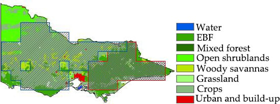
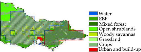
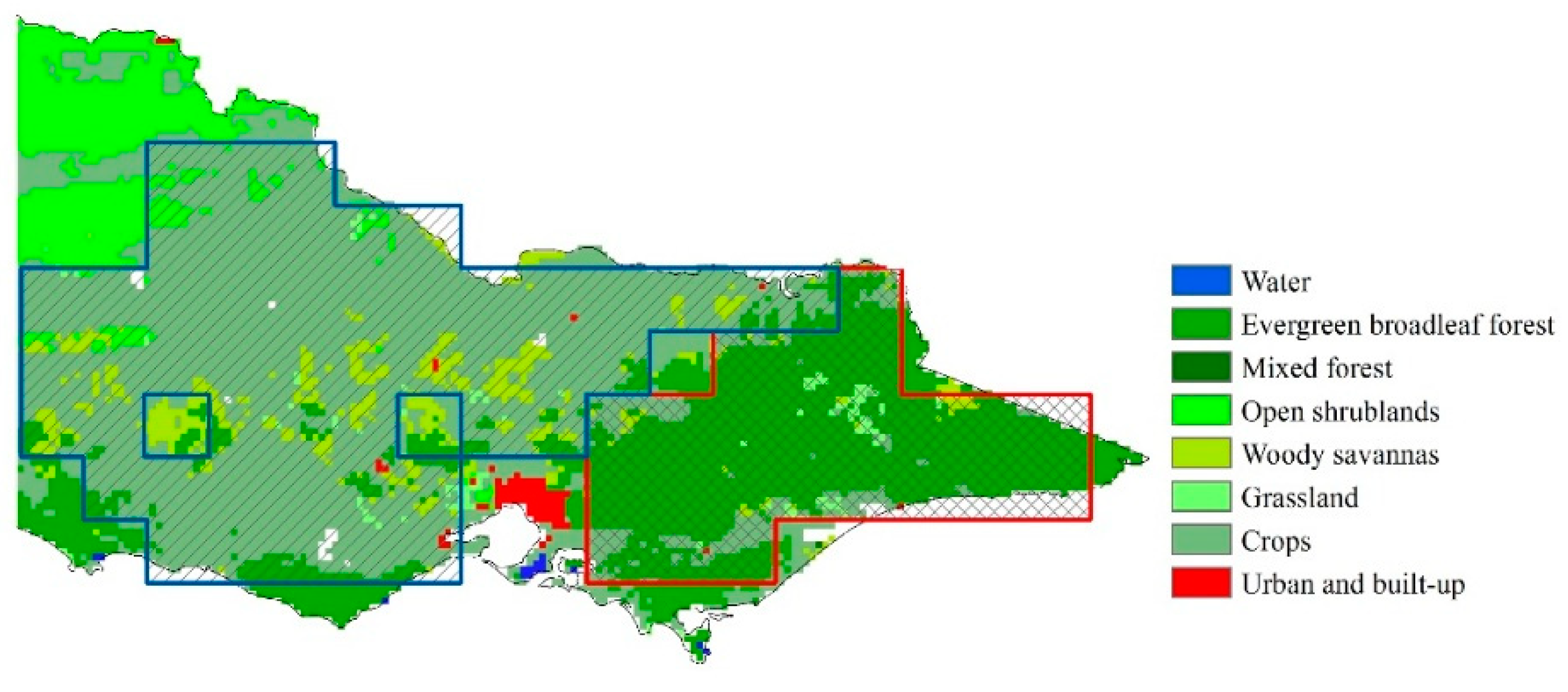
To analyze the potential biome-dependency of vegetation response to drought, we used land cover information derived from MODIS land cover product (MCD12C1, 2011, 0.05°). The land cover map in Victoria is shown in Figure 1. Crop and evergreen broadleaf forest consist of main land cover types in Victoria. 0.5° pixels were determined as crop land or evergreen broadleaf forest land if over 50% of the 0.05° pixels (i.e., more than 50 pixels) within the grid were identified as crop land or evergreen broadleaf forest land.

2.2. Meteorological Station Data

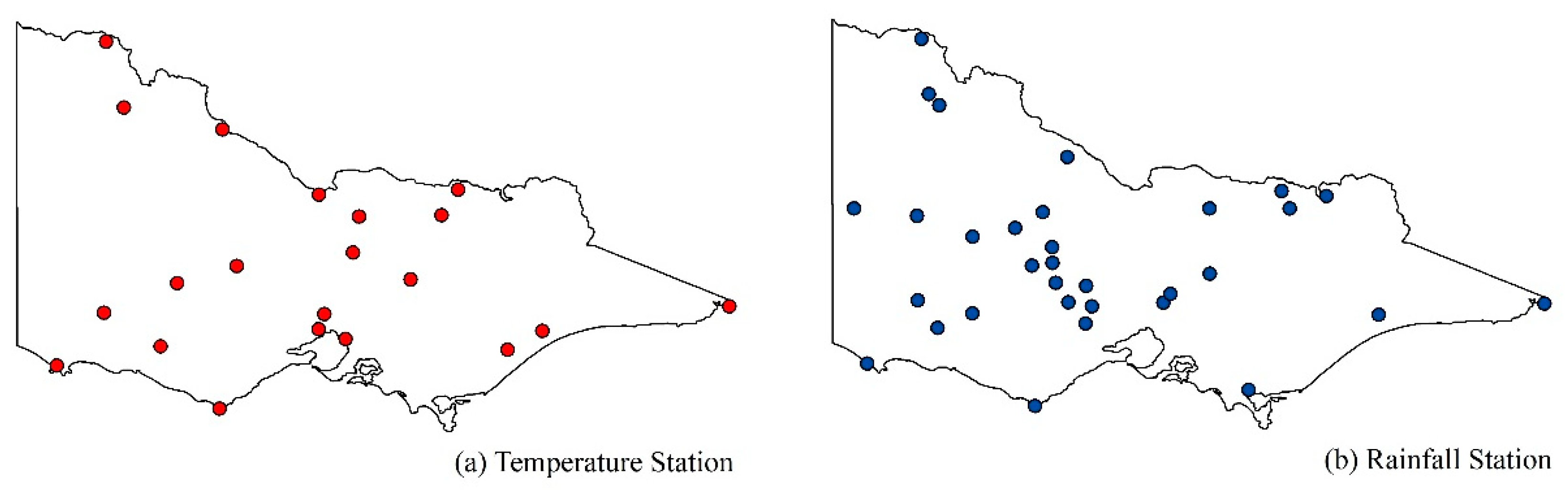
We used monthly mean maximum temperature (from 1982–2013) and monthly precipitation data (from 2007 to 2013), which were provided by the Australian Bureau of Meteorology, to represent drought-related environmental stress. Monthly mean maximum temperature was calculated as the average of all available daily maxima for the month. The highest observed temperature for the 24 hours before 09:00 local time was recorded as the daily maximum air temperature for the previous day. Monthly precipitation was calculated by summing all available daily rainfall records within the month, which include all forms of precipitation that reach the ground, such as rain, drizzle, hail, and snow. To represent the overall status of the meteorology in Victoria, we used data from 21 temperature stations and 32 precipitation stations. Detailed information of these stations is illustrated in Figure 2 and

Table A1. Temperature Stations.

Number	Site Name	Site Number	Latitude	Longitude
1	Mildura Airport	76031	142.0867	−34.2358
2	Ouyen (Post Office)	76047	142.3125	−35.0682
3	Swan Hill Post Office	77042	143.5533	−35.3406
4	Echuca Aerodrome	80015	144.7642	−36.1647
5	Tatura Institute of Sustainable Agriculture	81049	145.2672	−36.4378
6	Rutherglen Research	82039	146.5100	−36.1000
7	Wangaratta Aero	82138	146.3056	−36.4206
8	Gabo Island Lighthouse	84016	149.9200	−37.5700
9	East Sale Airport	85072	147.1322	−38.1156
10	Bairnsdale Airport	85279	147.5700	−37.8800
11	Moorabbin Airport	86077	145.0962	−37.9800
12	Melbourne Airport	86282	144.8321	−37.6655
13	Laverton Raaf	87031	144.7566	−37.8565
14	Lake Eildon	88023	145.9124	−37.2313
15	Maryborough	88043	143.7300	−37.0600
16	Mangalore Airport	88109	145.1900	−36.8900
17	Ararat Prison	89085	142.9786	−37.2769
18	Cape Otway Lighthouse	90015	143.5128	−38.8556
19	Portland (Cashmore Airport)	90171	141.4705	−38.3148
20	Hamilton Airport	90173	142.0600	−37.6500
21	Mortlake Racecourse	90176	142.7744	−38.0737

and

Table A2. Precipitation Stations.

Number	Site Name	Site Number	Latitude	Longitude
1	Kaniva	78078	141.2427	−36.3725
2	Mildura Airport	76031	142.0867	−34.2358
3	Nulkwyne Kiamal	76043	142.1800	−34.9300
4	Ouyen (Post Office)	76047	142.3100	−35.0700
5	Dimboola	78010	142.0327	−36.4644
6	Warranooke (Glenorchy)	79016	142.7303	−36.7281
7	St. Arnaud	79040	143.2644	−36.6175
8	Kerang	80023	143.9197	−35.7236
9	Wedderburn (Post Office)	80061	143.6123	−36.4183
10	Avoca (Post Office)	81000	143.4747	−37.0887
11	Dookie Agricultural College	81013	145.7048	−36.3717
12	Dunolly	81085	143.7295	−36.8593
13	Beechworth Composite	82001	146.7132	−36.3702
14	Chiltern (Post Office)	82010	146.6106	−36.1491
15	Tallangatta Dcnr	82045	147.1764	−36.2161
16	Bruthen (Post Office)	84003	147.8314	−37.7073
17	Gabo Island Lighthouse	84016	149.9158	−37.5679
18	Foster (Post Office)	85029	146.1997	−38.6520
19	Yan Yean	86131	145.1259	−37.5552
20	Ballan	87006	144.2295	−37.6018
21	Bungaree (Kirks Reservoir)	87014	143.9322	−37.5512
22	Meredith (Darra)	87043	144.1492	−37.8197
23	Alexandra (Post Office)	88001	145.7116	−37.1916
24	Clunes	88015	143.7776	−37.3049
25	Daylesford	88020	144.1575	−37.3432
26	Maryborough	88043	143.7320	−37.0560
27	Kinglake West (Wallaby Creek)	88060	145.2143	−37.4475
28	Cavendish (Post Office)	89009	142.0414	−37.5267
29	Wickliffe	89033	142.7253	−37.6901
30	Cape Bridgewater	90013	141.4060	−38.3215
31	Cape Otway Lighthouse	90015	143.5128	−38.8556
32	Penshurst (Post Office)	90063	142.2895	−37.8750

in Appendix A. The measured data were quality controlled using quality flags and were relatively uninterrupted.

3. Methods

We first analyzed the temporal and spatial dynamics of GPP, SIF, APAR_NDVI and APAR_EVI for the 2009 drought event and compared the drought responses of vegetation proxies for the main vegetation types in Victoria. We applied monthly relative anomalies and the normalized anomaly of all the aforementioned variables to assess drought stress-related signals. The relative anomaly ($\Delta$) and normalized anomaly ($\mathsf{\delta }$) can be calculated as below:

$$\Delta (i,k)=(\mathrm{P}\left(i,k\right)-{\mathrm{P}\left(i\right)}_{\mathrm{mean}}{)/\mathrm{P}(i)}_{\mathit{mean}}$$

(3)

$$\mathsf{\delta }(i,k)=(\mathrm{P}\left(i,k\right)-{\mathrm{P}\left(i\right)}_{\mathrm{mean}}{)/\mathrm{P}(i)}_{\mathit{std}}$$

(4)

where $\mathrm{P}\left(i,k\right)$ stands for different variables (e.g., GPP, SIF, APAR and other meteorological variables) for month i of year k, and the multiyear mean ${\mathrm{P}\left(i\right)}_{\mathit{mean}}$ and standard deviation ${\mathrm{P}\left(i\right)}_{\mathit{std}}$ are established from 2007 to 2013 for all data sets.

To further explore the feasibility of SIF in interpreting drought effects on vegetation productivity in Victoria, we estimated the response of vegetation to drought-related meteorology anomalies in a relatively long period (2007–2013). Because the sensitivity of vegetation productivity to high temperature is variable in different seasons [50], we first analyzed the relationship between the temperature from stations and GPP over 1982-2013 and obtained the annual-temperature-sensitive period when GPP decreased with increasing temperature. Based on the determined annual-temperature-sensitive period, we applied the autoregressive with exogenous terms (ARx) model [48,51] to estimate the sensitivities of GPP and vegetation proxies to meteorology anomalies and examined the correlations of the GPP anomaly with the anomalies of vegetation proxies. The ARx model is an auto-regressive model with exogenous inputs [51]. We used the GPP as an example to illustrate the ARx model:

$${\mathsf{\delta }\mathrm{GPP}}_{\mathrm{t}}={\mathrm{a}}^{\mathrm{T}}\times \mathsf{\delta }{\mathrm{T}}_{\mathrm{t}}+{\mathrm{a}}^{\mathrm{W}}\times \mathsf{\delta }{\mathrm{W}}_{\mathrm{t}}+{\mathrm{a}}^{\mathrm{P}}\times \mathsf{\delta }{\mathrm{P}}_{\mathrm{t}}+{\mathrm{a}}^{\mathrm{M}}\times \mathsf{\delta }{\mathrm{GPP}}_{\mathrm{t}-1}+\mathsf{\epsilon }$$

(5)

where ${\mathsf{\delta }\mathrm{GPP}}_{\mathrm{t}}$, ${\mathsf{\delta }\mathrm{T}}_{\mathrm{t}}$, ${\mathsf{\delta }\mathrm{W}}_{\mathrm{t}}$ and ${\mathsf{\delta }\mathrm{P}}_{\mathrm{t}}$ represent the normalized anomalies of GPP, ECMWF temperature, water availability and PAR, respectively, at month t; ${\mathsf{\delta }\mathrm{GPP}}_{\mathrm{t}-1}$ is the normalized GPP anomaly at month t-1. The one-month-lagged normalized GPP anomaly was used to investigate potential memory effects. Time series were normalized to assure comparability of the coefficients. ${\mathrm{a}}^{\mathrm{T}}$, ${\mathrm{a}}^{\mathrm{W}}$ and ${\mathrm{a}}^{\mathrm{P}}$ represent the estimated sensitivity of GPP changes to the respective meteorology-forcing factors while ${\mathrm{a}}^{\mathrm{M}}$ is related to memory effects and $\mathsf{\epsilon }$ is the residual error term. The coefficient of determination (R²) value of model result and the significance of the model’s coefficients were used to assess the quality of the fitting. We used the partial least squares method (PLS) to solve the parameters in Equation (5) to avoid multicollinearity of the forcing factors.

Note that all the analyses were made for general Victoria region, crop land and evergreen broadleaf forest land to consider potential different behaviors of different vegetation types during drought conditions.

4. Results

4.1. Monitoring and Assessing the 2009 Drought in Victoria

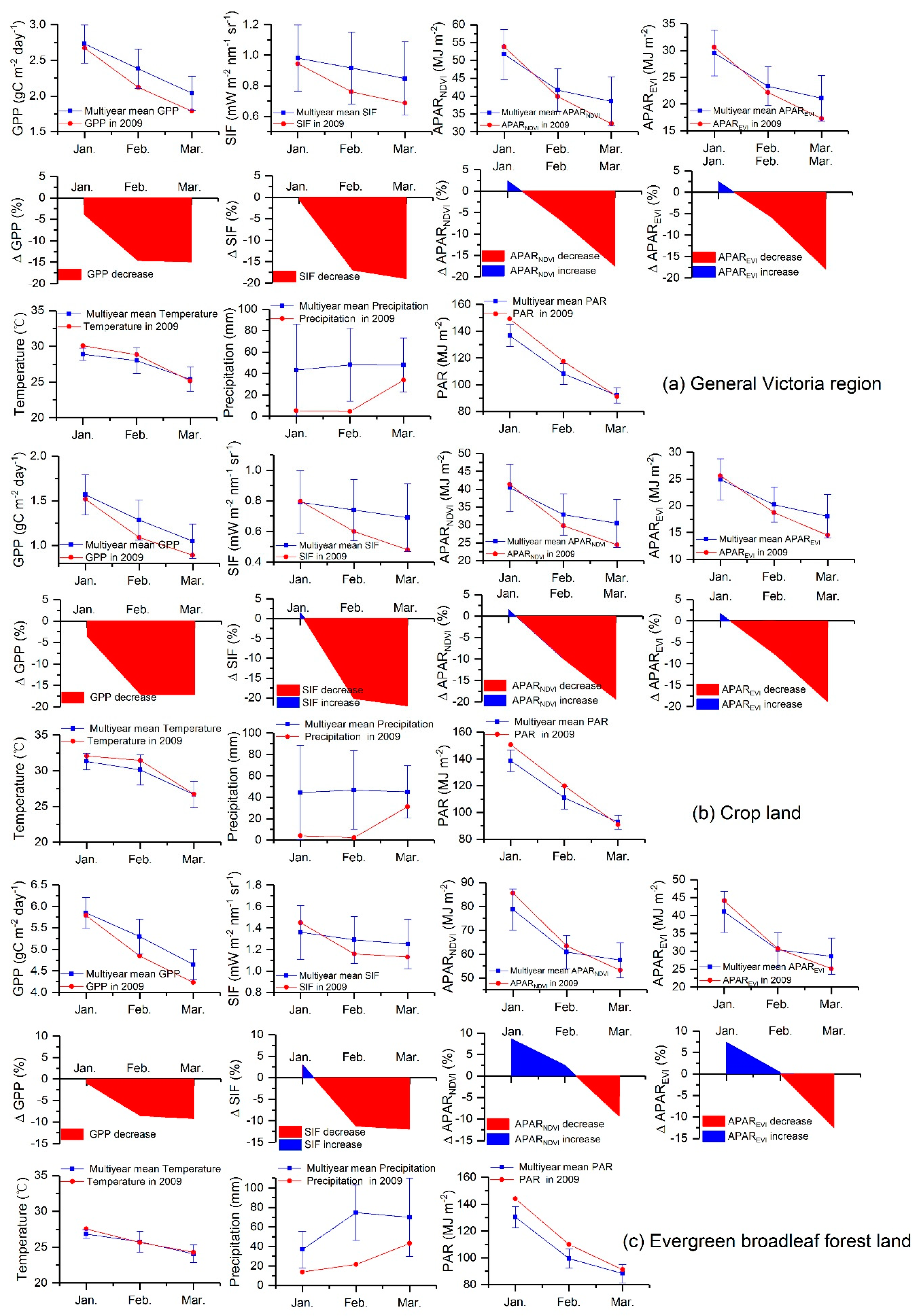
Figure 3 shows the temporal dynamics of all the studied variables during the 2009 drought period (from January to March) for general Victoria region (Figure 3a), crop land (Figure 3b) and evergreen broadleaf forest land (Figure 3c). According to Figure 3a, Victoria experienced a fairly higher temperature and a lower rainfall than the historical mean values in January 2009. The inter-annual precipitation variation is strong (large standard deviations), which indicates the extent of rainfall variation changes dramatically in Victoria. High temperatures and drops in precipitation rapidly depleted soil moisture through evapotranspiration, causing a severe reduction in vegetation productivity [27]. GPP, SIF, APAR_NDVI and APAR_EVI showed a decreasing tendency from January 2009 to March 2009. GPP and SIF from January to March for 2009 were lower than their historical averages for 2007–2013. On the contrary, both APAR_NDVI and APAR_EVI were slightly higher in January 2009 relative to their multiyear means. SIF decreased by approximately 17.2% in February 2009, which was much higher than the declines in APAR_NDVI (6.9%) and APAR_EVI (5.9%). The relative SIF and GPP anomalies decreased more sharply from January 2009 to February 2009 than did the relative APAR_NDVI and APAR_EVI anomalies from January to February for general Victoria region. For crop land (Figure 3b), SIF, APAR_NDVI and APAR_EVI showed similar relative anomalies in January 2009. Yet SIF decreased by approximately 20.1% in February 2009, which was higher than the observed decreases for APAR_NDVI (9.7%) and APAR_EVI (7.5%). Regarding evergreen broadleaf forest land (Figure 3c), APAR_NDVI and APAR_EVI exhibited positive relative anomalies in February 2009, while SIF decreased by approximately 11.3% and GPP decreased by approximately 8.5%. These results indicate that the relative GPP anomaly had a more consistent change with the relative SIF anomaly than with the relative APAR_NDVI and APAR_EVI anomalies, especially for evergreen broadleaf forest land.

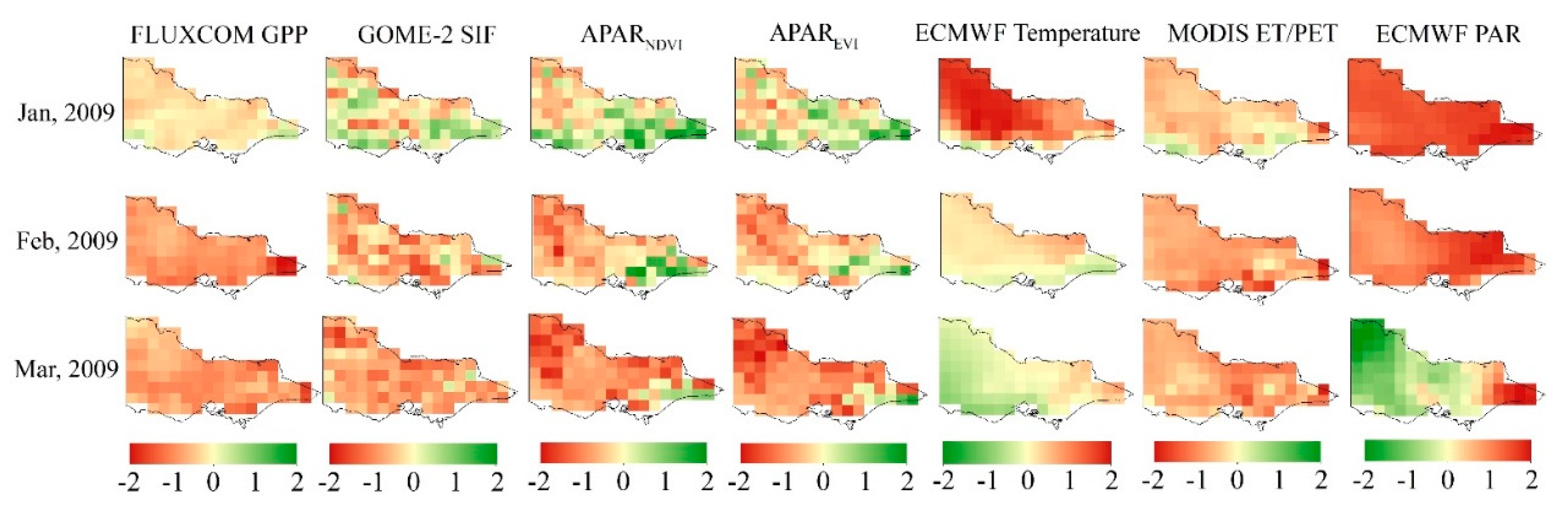
The spatial and temporal variations of the normalized anomalies of all the considered variables in Victoria from January to March 2009 are shown in Figure 4. It is seen that Victoria was struck by extremely high temperature in January 2009, and part of the Victoria area showed drought stress which was indicated by the normalized anomalies of vegetation proxies. In February 2009, the temperature was lower than the multiyear mean temperature while the water availability was still deficient, which indicates the persistence of drought stress in Victoria. Both GPP and SIF showed drought-induced anomalies in most areas of Victoria. In southeastern Victoria, where evergreen broadleaf forest consists of the main vegetation type (Figure 1), the normalized APAR_NDVI and APAR_EVI anomalies exhibited more positive anomalies than did SIF anomaly in February 2009. These results indicate that during the studied 2009 drought event, APAR_NDVI and APAR_EVI are less sensitive to meteorological drought stress compared with SIF in evergreen broadleaf forest land. In March 2009, drought stress was not completely alleviated. The normalized APAR_NDVI and APAR_EVI anomalies indicated that drought still persisted in Victoria except for most evergreen broadleaf forest areas.

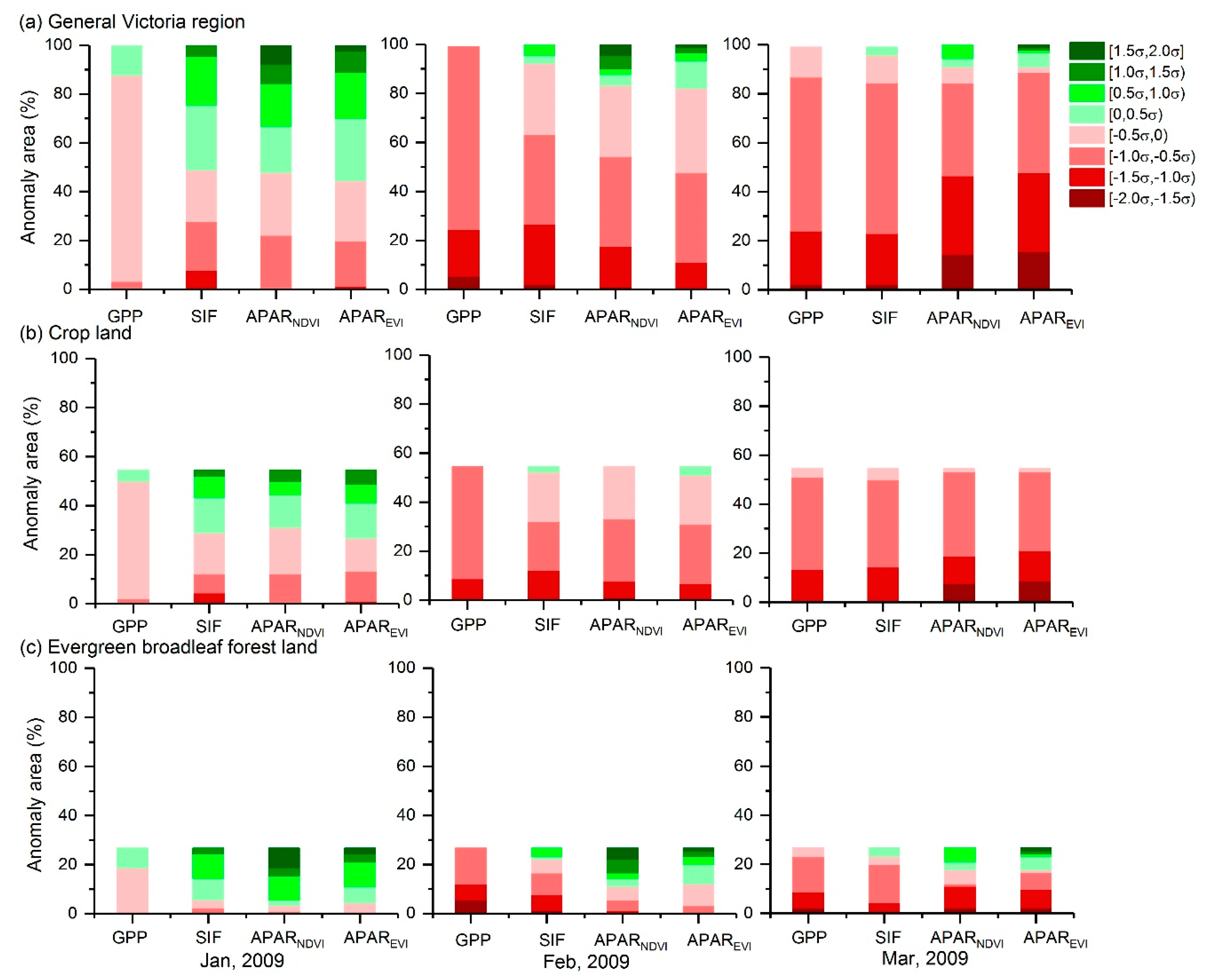
Figure 5 shows the statistics of anomalous areas calculated by the normalized GPP, SIF, APAR_NDVI and APAR_EVI anomalies based on the results, shown in Figure 4. Figure 5a shows the percentages of negative and positive anomaly areas calculated by all pixels located in the general region of Victoria. For moderate drought stress (< -0.5σ), the area percentage indicated by SIF (28.1%) was similar to those indicated by APAR_NDVI (22.5%) and APAR_EVI (20.2%) in January 2009. For severe positive anomaly (>1σ), however, the area percentage shown by APAR_NDVI was 15.6% and the value for APAR_EVI was 11.2%, while the values shown by SIF and GPP were 0%. For severe drought stress (<−1σ) in February 2009, the area percentage indicated by GPP was 24.7%, and the value for SIF was 27%. On the other hand, the values for APAR_NDVI (18.0%) and APAR_EVI (11.2%) were much smaller than those revealed by SIF and GPP. SIF showed more similarity to APAR_NDVI and APAR_EVI than to GPP for the drought stress of [-1σ, 0) in February. The area percentages for severe drought stress shown by APAR_NDVI and APAR_EVI were lower than those shown by SIF and GPP in February. In March, the area percentages of extreme drought stress (<−1.5σ) shown by APAR_NDVI (7.8%) and APAR_EVI (8.9%) were much higher than those shown by GPP and SIF.

Figure 5b,c show the percentages of negative and positive anomaly areas calculated by the pixels located in crop land and evergreen broadleaf forest land, respectively. For crop land, results for SIF, APAR_NDVI and APAR_EVI were overall consistent. In February, the area percentage of severe drought stress (<−1σ) shown by SIF was higher than those shown by APAR_NDVI and APAR_EVI. In March, the area percentages of extreme drought stress (<−1.5σ) shown by APAR_NDVI and APAR_EVI were 7.8% and 8.9%, respectively, while no extreme drought-stressed area was indicated by GPP or SIF. Regarding evergreen broadleaf forest land, APAR_NDVI and APAR_EVI showed positive anomalies and SIF exhibited a high area percentage for the weak positive anomaly of [0, 1σ) in January. In February, the area percentage of the drought stress (<0) shown by SIF was higher than those shown by APAR_NDVI and APAR_EVI. In March, APAR_NDVI and APAR_EVI showed more severe drought losses (<−1σ) than did SIF and GPP.

4.2. General Analyses of the Responses of FLUXCOM GPP, SIF, APAR_NDVI and APAR_EVI to Drought

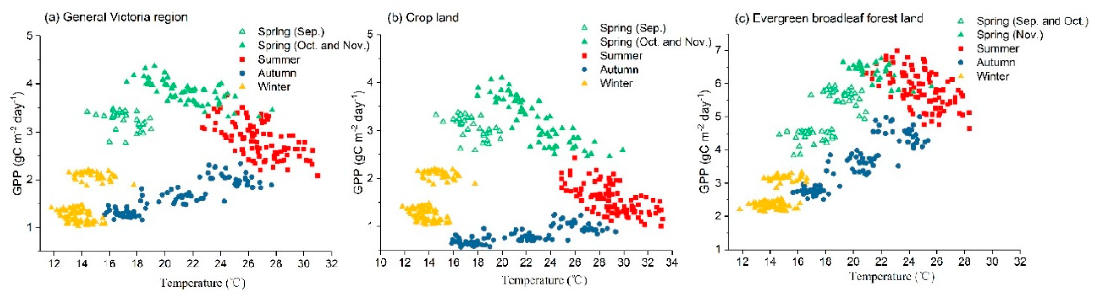
In this section, we explored the sensitivities of GPP and vegetation proxies to drought-related meteorology anomalies using the ARx model. Since the sensitivity of vegetation productivity to high temperature is variable in different seasons [50], we first analyzed the relationships between GPP and temperature based on data from 1982 to 2013 to obtain the annual-temperature-sensitive period. Figure 6 shows distinct seasonal features between the temperature and GPP for the general region of Victoria (Figure 6a), crop land (Figure 6b) and evergreen broadleaf forest land (Figure 6c). It is shown that the distribution of data points in GPP-temperature space is similar to a triangle, and GPP showed contrasting responses to temperature in different seasons. For the general area of Victoria, GPP decreases with increasing temperature in late spring (i.e., October and November) and summer. The vegetation productivity is slightly enhanced in autumn and barely changes in winter by increased temperature. The period with the highest GPP-temperature sensitivity is from October to February. The feature of crop land is similar to the result generated for the general region of Victoria. For evergreen broadleaf forest land, the annual-temperature-sensitive period when GPP decreased by increased temperature is from November to February.

Based on the annual-temperature-sensitive period, we explored the impacts of temperature, water availability and PAR on vegetation activity indicated by GPP and vegetation proxies using the ARx model regarding memory effects. The sensitivities of these vegetation variables (e.g., GPP, SIF, APAR_NDVI and APAR_EVI) anomalies to temperature, water availability, PAR and the one-month-lagged vegetation activity are respectively represented by ${\mathrm{a}}^{\mathrm{T}}$, ${\mathrm{a}}^{\mathrm{W}}$, ${\mathrm{a}}^{\mathrm{P}}$ and ${\mathrm{a}}^{\mathrm{M}}$, respectively. The ARx model output results for general Victoria region, crop land and evergreen broadleaf forest land are shown in

Table 1. Parameters of the ARx models for general Victoria region, crop land and evergreen broadleaf forest land in Victoria. Results are only based on data only for the annual-temperature-sensitive period (i.e., from October to February for the general Victoria region and crop land and from November to February for evergreen broadleaf forest land) from 2007 to 2013. “*”, “**” and “***” represent 0.1, 0.05 and 0.01 significant levels, respectively.

Vegetation variables	Parameters of the ARx Model for General Victoria Region
	aT	aW	aP	aM	R2	RMSE	p Value
GPP	−0.24 ***	0.29 ***	−0.25 ***	0.23 ***	0.75	0.51	0.00
SIF	−0.22 **	0.28 ***	−0.25 *	0.24 *	0.72	0.35	0.00
APARNDVI	−0.16	0.26 *	−0.13 *	0.16 **	0.29	0.78	0.01
APAREVI	−0.11	0.24 **	−0.08 *	0.11	0.20	0.83	0.21
Vegetation variables	Parameters of the ARx Model for Crop Land in Victoria
	aT	aW	aP	aM	R2	RMSE	p Value
GPP	−0.19 ***	0.32 ***	−0.26 ***	0.27 ***	0.77	0.48	0.00
SIF	−0.17 ***	0.32 ***	−0.24 ***	0.23 ***	0.61	0.63	0.00
APARNDVI	−0.16 **	0.31 ***	−0.15 *	0.16 *	0.38	0.77	0.01
APAREVI	−0.13 *	0.26 **	−0.08	0.12	0.20	0.79	0.34
Vegetation variables	Parameters of the ARx Model for Evergreen Broadleaf Forest Land in Victoria
	aT	aW	aP	aM	R2	RMSE	p Value
GPP	−0.17 *	0.27 ***	−0.28 ***	0.18 **	0.48	0.71	0.01
SIF	−0.10	0.22 *	−0.23 *	0.22	0.36	0.50	0.01
APARNDVI	0.17	0.70	0.60	0.53	0.19	0.64	0.07
APAREVI	0.24	0.97	0.62	0.44	0.33	0.45	0.46

. The aforementioned variables anomalies have been standardized using z-score standardization to assure comparability between the coefficients in the ARx model.

Both GPP and SIF exhibit high levels of confidence, and the low root mean square error (RMSE) for general Victoria region. SIF gains the highest model precision (R² = 0.72) compared with APAR_NDVI (R² = 0.29) and APAR_EVI (R² = 0.20). It is interpreted that both GPP and SIF anomalies can be explained by meteorology anomalies and memory effects. ${\mathrm{a}}^{\mathrm{T}}$ estimated by SIF is more significant than those estimated by APAR_NDVI and APAR_EVI. ${\mathrm{a}}^{\mathrm{P}}$ exhibits negative effects on vegetation activity. ${\mathrm{a}}^{\mathrm{W}}$ estimated by all the vegetation variables are similar in the ARx model. ${\mathrm{a}}^{\mathrm{M}}$ indicated by GPP, SIF and APAR_NDVI are significant. It is interpreted that memory effects also have important impacts on vegetation productivity compared with other meteorology factors. The sensitivities of theses vegetation variables anomalies to water availability anomalies are stronger than those to temperature and PAR anomalies. Therefore, water availability is regarded as an important meteorology-forcing factor for plant activity during October-February in the studied area. These results agree well with the previous study that investigated water limitation and vegetation memory effects in Victoria [48].

Regarding crop land, GPP and SIF exhibit similar results (high levels of confidence and low RMSE) to those generated for general Victoria region. It is interpreted that both GPP and SIF variations can be explained by meteorology anomalies in crop land. ${\mathrm{a}}^{\mathrm{T}}$ and ${\mathrm{a}}^{\mathrm{W}}$ indicated by APAR_NDVI and APAR_EVI are significant (p < 0.1) in crop land. In contrast, none of the coefficients for APAR_NDVI and APAR_EVI are significant for evergreen broadleaf forest land. Thus, APAR_NDVI and APAR_EVI anomalies cannot be estimated by meteorology anomalies in evergreen broadleaf forest land. For evergreen broadleaf forest land, the coefficients ${\mathrm{a}}^{\mathrm{T}}$ and ${\mathrm{a}}^{\mathrm{M}}$ indicated by SIF are not significant. ${\mathrm{a}}^{\mathrm{W}}$ and ${\mathrm{a}}^{\mathrm{P}}$ generated by SIF are more significant than those indicated by APAR_NDVI and APAR_EVI. This result indicates that SIF can be explained by water availability and PAR to some degree in evergreen broadleaf forest land.

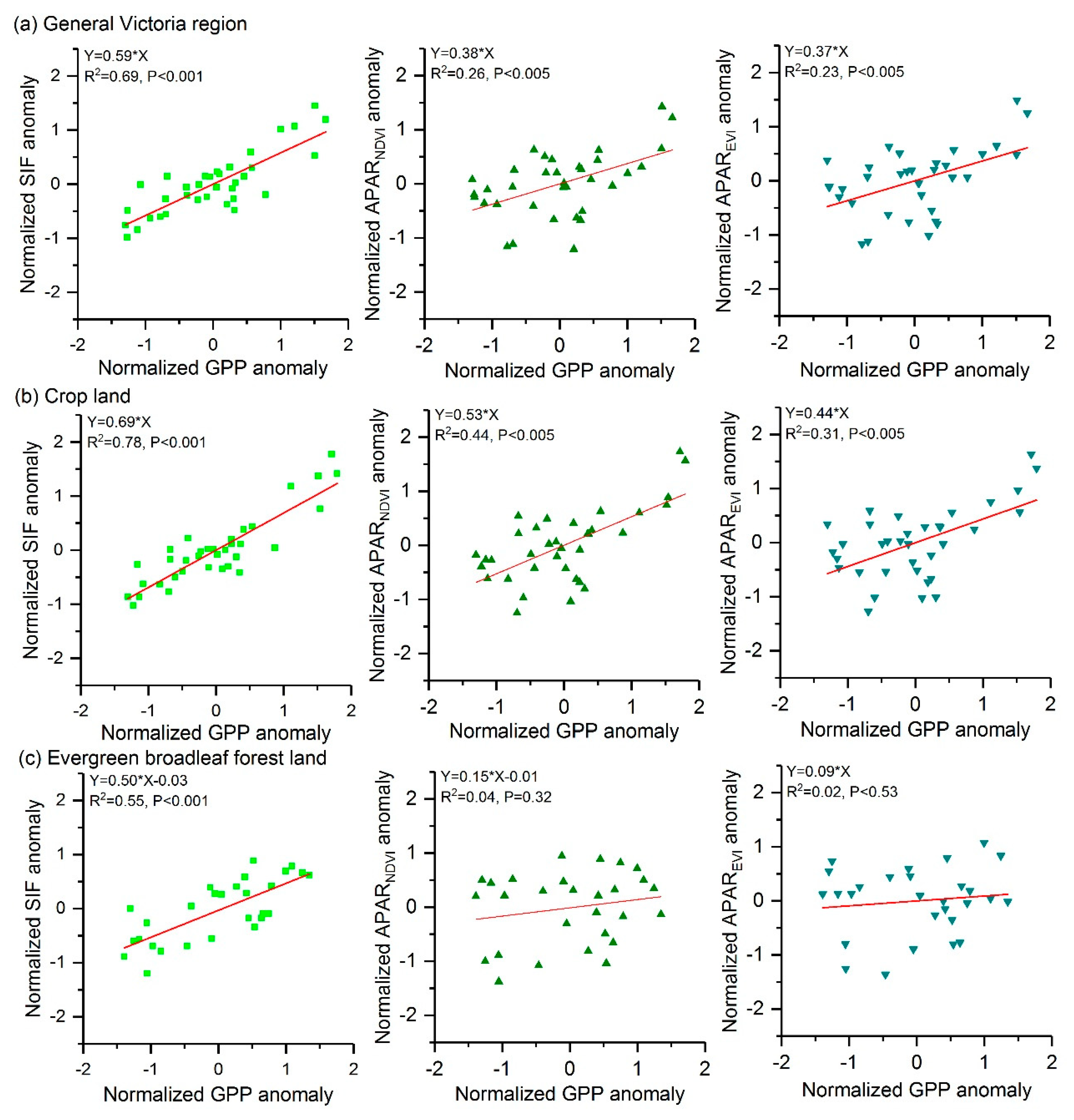
To further explore the consistency of GPP and vegetation proxies under drought conditions, we compared the correlations between the normalized GPP anomaly and the normalized anomalies of vegetation proxies for general Victoria and different land types (Figure 7). It is shown by Figure 7 that strong correlations between the normalized SIF anomaly and the normalized GPP anomaly can be found for general Victoria, crop land area and evergreen broadleaf forest land area. Compared with SIF anomaly, APAR_NDVI and APAR_EVI anomalies not only show worse correlations to GPP anomaly, but also exhibit lower slopes of regressions to GPP anomaly. These results indicate that SIF anomaly is more sensitive to changes in GPP anomaly than are APAR_NDVI and APAR_EVI. In general, anomalies of vegetation proxies exhibit stronger correlation with GPP anomaly in crop land than in evergreen broadleaf forest land.

5. Discussion

SIF showed a much larger decrease, which was consistent with GPP declines, than did APAR_NDVI and APAR_EVI during the 2009 drought event (Figure 3). According to Equation (2), SIF decrease is expected to be induced by both APAR (or FPAR) and ${\mathsf{\epsilon }}_{\mathrm{F}}$ losses [27], while changes in APAR_NDVI and APAR_EVI are induced by PAR and FPAR estimated by VIs. For the 2009 drought event, PAR showed positive anomalies in January and February. It is interpreted that negative precipitation anomalies are often accompanied by positive PAR anomalies during the drought period, due to less cloud [52]. Besides, greenness-related VIs have no direct link to photosynthetic function beyond their sensitivity to canopy structure and pigment concentration [20]. The responses of VIs to drought may be different, because changes in vegetation canopy vary across different biomes under drought conditions [11]. In February 2009 (Figure 4), APAR_NDVI and APAR_EVI anomalies did not reflect the drought-induced vegetation productivity losses in southeastern Victoria, where evergreen broadleaf forest consists of the main land cover type. For evergreen broadleaf forest ecosystems, canopy changes are minor and GPP anomalies mainly come from the ${\mathsf{\epsilon }}_{\mathrm{P}}$ limitations on the photosynthetic activities during drought conditions [11]. However, canopy changes are dominant for non-forest ecosystems under drought stress [11,53]. Previous studies have shown that the leaf area index (LAI) has a good correlation with GPP under drought conditions in non-forest ecosystems [11,53]. Thus, VIs related to the properties of vegetation canopy and leaf greenness can better reflect the vegetation productivity anomalies of crops than those of evergreen broadleaf forest [54]. The ARx model provides an indication of the short-term impacts of meteorology anomalies on vegetation productivity, including memory effects. In Table 1, memory effects to GPP and SIF cannot be ignored compared to meteorology stress. It is interpreted that anomalies in vegetation productivity might result from either past meteorology anomalies or current stress conditions [51]. The values of ${\mathrm{a}}^{\mathrm{M}}$ and ${\mathrm{a}}^{\mathrm{T}}$ induced by APAR_NDVI are similar for general Victoria region and crop land. These results are consistent with the results of GPP and SIF. ${\mathrm{a}}^{\mathrm{W}}$ estimated by GPP and SIF in crop land are higher than in evergreen broadleaf forest land. It indicates that the sensitivity of crops to water availability is stronger than that of evergreen broadleaf forest. This result might be related to the different resistances to water availability between crop and forest ecosystems. Forest ecosystems have deeper roots and a higher capability to utilize soil water compared with crop ecosystems [11]. Therefore, forest ecosystems are more resistant to water stress than are crop ecosystems. In general, SIF anomaly can be explained by the combined stress from temperature, water availability and PAR for general Victoria region and crop land. The sensitivity of SIF to meteorology anomalies provides its potential superiority for monitoring vegetation productivity variations accurately under drought conditions.

SIF anomaly showed a stronger linear relationship with GPP anomaly than did APAR anomalies (Figure 7). This result may be related to the relationship between ${\mathsf{\epsilon }}_{\mathrm{P}}$ and ${\mathsf{\epsilon }}_{\mathrm{F}}$. Verma et al. [41] reported a strong linear relationship between ${\mathsf{\epsilon }}_{\mathrm{F}}$ and ${\mathsf{\epsilon }}_{\mathrm{P}}$. According to Equations (1) and (2), although both SIF and APAR are responsive to FPAR, which is related to chlorophyll content and LAI, SIF, but not APAR, is sensitive to variations in ${\mathsf{\epsilon }}_{\mathrm{F}}$. Therefore, GPP anomaly has a better consistency with SIF anomaly than with APAR anomalies.

SIF was retrieved using a simplified radiative transfer model together with a principal component (PC) analysis to disentangle the spectral signatures of atmospheric absorption, surface reflectance and fluorescence emission. [42,43]. Previous studies have discussed the effect of the fit window, the numbers of PCs, and the reference area for PC determination on the retrieval outcome [42,43,55]. Köhler et al. depicted the standard error of the mean of GOME-2 SIF composites for January 2011, and the results showed that the standard error of the mean was generally low (<0.15 mW/m²/sr/nm) for GOME-2 SIF in Australia [42]. The coarse-spatial- and low-temporal-resolution data source for SIF can constrain its potential. The feasibility of SIF should be further investigated using data with a higher spatio-temporal resolution in the future [56].

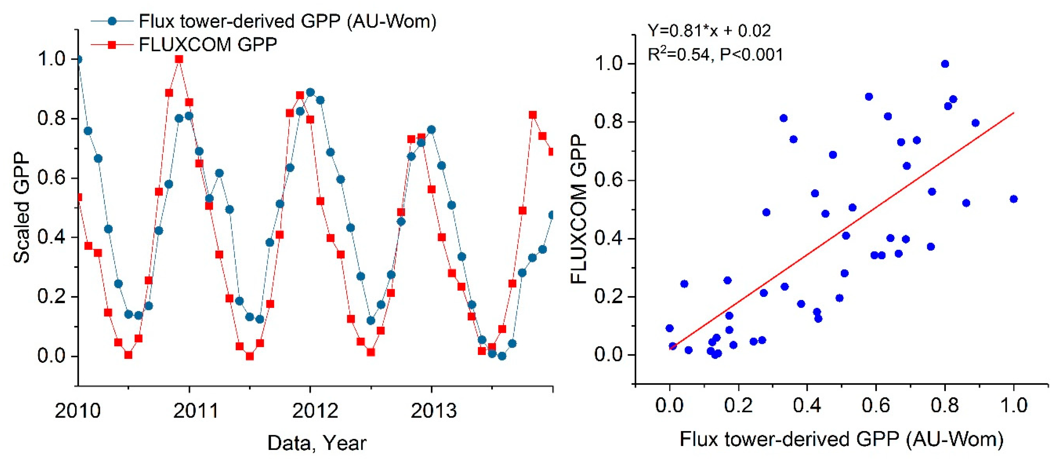
It has been reported that FLUXCOM GPP data contain uncertainty regarding the evergreen broadleaf forest land (especially in the Amazon and Indonesia) [44]. To evaluate the quality of the regional GPP product used in this study, especially for evergreen broadleaf forest land in Victoria, we validated FLUXCOM GPP against eddy-covariance-based GPP estimations (Appendix B Figure A1). The results indicate that the change tendency of FLUXCOM GPP is similar to that of flux tower-derived GPP. Overall, FLUXCOM GPP can be used to investigate the effects of meteorology anomalies on vegetation productivity [45] and capture the considerable drawdown of vegetation activities during the 2009 drought event in Victoria.

6. Conclusions

In this study, we analyzed the responses of GPP, SIF, APAR_NDVI and APAR_EVI to drought during the 2009 drought event in Victoria. For general Victoria region, satellite SIF had a more consistent decline with GPP losses induced by drought stress than did APAR_NDVI and APAR_EVI. We also analyzed and compared the responses of these vegetation variables to drought for the main vegetation types in Victoria. APAR_NDVI and APAR_EVI had obvious lagged responses compared with SIF in evergreen broadleaf forest land. The spatial and temporal pattern results indicate that the sensitivity of SIF to drought is stronger than those of APAR_NDVI and APAR_EVI for this 2009 drought event in Victoria.

To better illustrate the applicability of SIF for monitoring drought effects, we estimated the sensitivities of vegetation variables to meteorology anomalies using the ARx model, and analyzed the consistency of GPP anomaly and vegetation proxies anomalies for the main ecosystem types in Victoria. The ARx model results indicate that GPP and SIF are more sensitive to temperature stress for general Victoria region than are APAR anomalies. Compared with APAR anomalies, SIF anomaly can be explained better by meteorology anomalies for evergreen broadleaf forest land. In addition, GPP anomaly has a more significant relationship with SIF anomaly than with APAR_NDVI and APAR_EVI anomalies, especially in evergreen broadleaf forest land. Thus, SIF can accurately track and evaluate vegetation productivity variations under meteorology stress. SIF provides a powerful tool for accurately monitoring and assessing the response of plant productivity to drought.

References

- Evans, B.J.; Lyons, T. Bioclimatic extremes drive forest mortality in southwest, Western Australia. Climate 2013, 1, 28–52. [Google Scholar] [CrossRef]
- Zhao, M.; Running, S.W. Drought-Induced Reduction in Global Terrestrial Net Primary Production from 2000 Through 2009. Science 2010, 329, 940–943. [Google Scholar] [CrossRef] [PubMed]
- Lewis, S.L.; Brando, P.M.; Phillips, O.L.; van der Heijden, G.M.F.; Nepstad, D. The 2010 Amazon Drought. Science 2011, 331, 554. [Google Scholar] [CrossRef] [PubMed]
- Gibbs, W. The great Australian drought: 1982–1983. Disasters 1984, 8, 89–104. [Google Scholar] [CrossRef] [PubMed]
- Rice, K.J.; Matzner, S.L.; Byer, W.; Brown, J.R. Patterns of tree dieback in Queensland, Australia: The importance of drought stress and the role of resistance to cavitation. Oecologia 2004, 139, 190–198. [Google Scholar] [CrossRef]
- van Dijk, A.I.; Beck, H.E.; Crosbie, R.S.; de Jeu, R.A.; Liu, Y.Y.; Podger, G.M.; Timbal, B.; Viney, N.R. The Millennium Drought in southeast Australia (2001–2009): Natural and human causes and implications for water resources, ecosystems, economy, and society. Water Resour. Res. 2013, 49, 1040–1057. [Google Scholar] [CrossRef]
- Centre, N.C. The exceptional January-February 2009 heatwave in southeastern Australia. Bur. Meteorol. 2009, 17, 2–3. [Google Scholar]
- Department of Climate Change and Energy Efficiency, A.G. Wildfire in forests in Australia. Available online: http://www.climatechange.gov.au/emissions (accessed on 26 April 2017).
- Meehl, G.A.; Tebaldi, C. More intense, more frequent, and longer lasting heat waves in the 21st century. Science 2004, 305, 994–997. [Google Scholar] [CrossRef]
- Pachauri, R.K.; Meyer, L.; Plattner, G.-K.; Stocker, T. IPCC, 2014: Climate Change 2014: Synthesis Report. Contribution of Working Groups I, II and III to the Fifth Assessment Report of the Intergovernmental Panel on Climate Change; IPCC: Geneva, Switzerland, 2015. [Google Scholar]
- Zhang, Y.; Xiao, X.M.; Zhou, S.; Ciais, P.; McCarthy, H.; Luo, Y.Q. Canopy and physiological controls of GPP during drought and heat wave. Geophys. Res. Lett. 2016, 43, 3325–3333. [Google Scholar] [CrossRef]
- Zeng, F.-W.; Collatz, G.; Pinzon, J.; Ivanoff, A. Evaluating and Quantifying the Climate-Driven Interannual Variability in Global Inventory Modeling and Mapping Studies (GIMMS) Normalized Difference Vegetation Index (NDVI3g) at Global Scales. Remote Sens. 2013, 5, 3918–3950. [Google Scholar] [CrossRef] [Green Version]
- Gu, Y.; Brown, J.F.; Verdin, J.P.; Wardlow, B. A five-year analysis of MODIS NDVI and NDWI for grassland drought assessment over the central Great Plains of the United States. Geophys. Res. Lett. 2007, 34. [Google Scholar] [CrossRef] [Green Version]
- Brouwers, N.C.; van Dongen, R.; Matusick, G.; Coops, N.C.; Strelein, G.; Hardy, G. Inferring drought and heat sensitivity across a Mediterranean forest region in southwest Western Australia: A comparison of approaches. Forestry 2015, 88, 454–464. [Google Scholar] [CrossRef]
- Kogan, F.N. Droughts of the late 1980s in the United States as derived from NOAA polar-orbiting satellite data. Bull. Am. Meteorol. Soc. 1995, 76, 655–668. [Google Scholar] [CrossRef]
- Rhee, J.; Im, J.; Carbone, G.J. Monitoring agricultural drought for arid and humid regions using multi-sensor remote sensing data. Remote Sens. Environ. 2010, 114, 2875–2887. [Google Scholar] [CrossRef]
- Huete, A.; Didan, K.; Miura, T.; Rodriguez, E.P.; Gao, X.; Ferreira, L.G. Overview of the radiometric and biophysical performance of the MODIS vegetation indices. Remote Sens. Environ. 2002, 83, 195–213. [Google Scholar] [CrossRef]
- Xu, L.A.; Samanta, A.; Costa, M.H.; Ganguly, S.; Nemani, R.R.; Myneni, R.B. Widespread decline in greenness of Amazonian vegetation due to the 2010 drought. Geophys. Res. Lett. 2011, 38. [Google Scholar] [CrossRef] [Green Version]
- Brede, B.; Verbesselt, J.; Dutrieux, L.P.; Herold, M. Performance of the enhanced vegetation index to detect inner-annual dry season and drought impacts on amazon forest canopies. In Proceedings of the 36th International Symposium on Remote Sensing of Environment, Berlin, Germany, 11–15 May 2015; Schreier, G., Skrovseth, P.E., Staudenrausch, H., Eds.; Volume 47, pp. 337–344. [Google Scholar]
- Soudani, K.; Hmimina, G.; Delpierre, N.; Pontailler, J.-Y.; Aubinet, M.; Bonal, D.; Caquet, B.; De Grandcourt, A.; Burban, B.; Flechard, C. Ground-based Network of NDVI measurements for tracking temporal dynamics of canopy structure and vegetation phenology in different biomes. Remote Sens. Environ. 2012, 123, 234–245. [Google Scholar] [CrossRef]
- Lloret, F.; Lobo, A.; Estevan, H.; Maisongrande, P.; Vayreda, J.; Terradas, J. Woody plant richness and NDVI response to drought events in Catalonian (northeastern Spain) forests. Ecology 2007, 88, 2270–2279. [Google Scholar] [CrossRef]
- Rossini, M.; Nedbal, L.; Guanter, L.; Ač, A.; Alonso, L.; Burkart, A.; Cogliati, S.; Colombo, R.; Damm, A.; Drusch, M.; et al. Red and far red Sun-induced chlorophyll fluorescence as a measure of plant photosynthesis. Geophys. Res. Lett. 2015, 42, 1632–1639. [Google Scholar] [CrossRef] [Green Version]
- Grace, J.; Nichol, C.; Disney, M.; Lewis, P.; Quaife, T.; Bowyer, P. Can we measure terrestrial photosynthesis from space directly, using spectral reflectance and fluorescence? Glob. Chang. Biol. 2007, 13, 1484–1497. [Google Scholar] [CrossRef]
- van der Tol, C.; Berry, J.A.; Campbell, P.K.; Rascher, U. Models of fluorescence and photosynthesis for interpreting measurements of solar-induced chlorophyll fluorescence. J. Geophys. Res. Biogeosci. 2014, 119, 2312–2327. [Google Scholar] [CrossRef] [PubMed] [Green Version]
- Song, L.; Guanter, L.; Guan, K.; You, L.; Huete, A.; Ju, W.; Zhang, Y. Satellite sun-induced chlorophyll fluorescence detects early response of winter wheat to heat stress in the Indian Indo-Gangetic Plains. Glob. Chang. Biol. 2018. [Google Scholar] [CrossRef]
- Yoshida, Y.; Joiner, J.; Tucker, C.; Berry, J.; Lee, J.E.; Walker, G.; Reichle, R.; Koster, R.; Lyapustin, A.; Wang, Y. The 2010 Russian drought impact on satellite measurements of solar-induced chlorophyll fluorescence: Insights from modeling and comparisons with parameters derived from satellite reflectances. Remote Sens. Environ. 2015, 166, 163–177. [Google Scholar] [CrossRef]
- Sun, Y.; Fu, R.; Dickinson, R.; Joiner, J.; Frankenberg, C.; Gu, L.; Xia, Y.; Fernando, N. Drought onset mechanisms revealed by satellite solar-induced chlorophyll fluorescence: Insights from two contrasting extreme events. J. Geophys. Res. Biogeosci. 2015, 120, 2427–2440. [Google Scholar] [CrossRef] [Green Version]
- Lee, J.E.; Frankenberg, C.; van der Tol, C.; Berry, J.A.; Guanter, L.; Boyce, C.K.; Fisher, J.B.; Morrow, E.; Worden, J.R.; Asefi, S.; et al. Forest productivity and water stress in amazonia: Observations from gosat chlorophyll fluorescence. Proc. Biol. Sci. 2013, 280, 20130171. [Google Scholar] [CrossRef] [PubMed]
- Wohlfahrt, G.; Gerdel, K.; Migliavacca, M.; Rotenberg, E.; Tatarinov, F.; Müller, J.; Hammerle, A.; Julitta, T.; Spielmann, F.; Yakir, D. Sun-induced fluorescence and gross primary productivity during a heat wave. Sci. Rep. 2018, 8, 14169. [Google Scholar] [CrossRef]
- Guanter, L.; Zhang, Y.; Jung, M.; Joiner, J.; Voigt, M.; Berry, J.A.; Frankenberg, C.; Huete, A.R.; Zarco-Tejada, P.; Lee, J.E.; et al. Global and time-resolved monitoring of crop photosynthesis with chlorophyll fluorescence. Proc. Natl. Acad. Sci. USA 2014, 111, E1327–E1333. [Google Scholar] [CrossRef] [PubMed] [Green Version]
- Wagle, P.; Xiao, X.; Torn, M.S.; Cook, D.R.; Matamala, R.; Fischer, M.L.; Jin, C.; Dong, J.; Biradar, C. Sensitivity of vegetation indices and gross primary production of tallgrass prairie to severe drought. Remote Sens. Environ. 2014, 152, 1–14. [Google Scholar] [CrossRef]
- Liu, L.; Guan, L.; Liu, X. Directly estimating diurnal changes in GPP for C3 and C4 crops using far-red sun-induced chlorophyll fluorescence. Agric. For. Meteorol. 2017, 232, 1–9. [Google Scholar] [CrossRef]
- Wagle, P.; Zhang, Y.; Jin, C.; Xiao, X. Comparison of solar-induced chlorophyll fluorescence, light-use efficiency, and process-based GPP models in maize. Ecol. Appl. 2016, 26, 1211–1222. [Google Scholar] [CrossRef] [PubMed]
- Yang, X.; Tang, J.; Mustard, J.F.; Lee, J.E.; Rossini, M.; Joiner, J.; Munger, J.W.; Kornfeld, A.; Richardson, A.D. Solar-induced chlorophyll fluorescence that correlates with canopy photosynthesis on diurnal and seasonal scales in a temperate deciduous forest. Geophys. Res. Lett. 2015, 42, 2977–2987. [Google Scholar] [CrossRef] [Green Version]
- Porcar-Castell, A.; Tyystjarvi, E.; Atherton, J.; van der Tol, C.; Flexas, J.; Pfundel, E.E.; Moreno, J.; Frankenberg, C.; Berry, J.A. Linking chlorophyll a fluorescence to photosynthesis for remote sensing applications: Mechanisms and challenges. J. Exp. Bot. 2014, 65, 4065–4095. [Google Scholar] [CrossRef] [PubMed]
- van der Molen, M.K.; Dolman, A.J.; Ciais, P.; Eglin, T.; Gobron, N.; Law, B.E.; Meir, P.; Peters, W.; Phillips, O.L.; Reichstein, M. Drought and ecosystem carbon cycling. Agric. For. Meteorol. 2011, 151, 765–773. [Google Scholar] [CrossRef]
- Flexas, J.; Escalona, J.M.; Evain, S.; Gulías, J.; Moya, I.; Osmond, C.B.; Medrano, H. Steady-state chlorophyll fluorescence (Fs) measurements as a tool to follow variations of net CO2 assimilation and stomatal conductance during water-stress in C3 plants. Physiol. Plant. 2002, 114, 231–240. [Google Scholar] [CrossRef] [PubMed]
- Daumard, F.; Champagne, S.; Fournier, A.; Goulas, Y.; Ounis, A.; Hanocq, J.-F.; Moya, I. A field platform for continuous measurement of canopy fluorescence. IEEE Trans. Geosci. Remote Sens. 2010, 48, 3358–3368. [Google Scholar] [CrossRef]
- Wang, S.; Huang, C.; Zhang, L.; Lin, Y.; Cen, Y.; Wu, T. Monitoring and Assessing the 2012 Drought in the Great Plains: Analyzing Satellite-Retrieved Solar-Induced Chlorophyll Fluorescence, Drought Indices, and Gross Primary Production. Remote Sens. 2016, 8, 61. [Google Scholar] [CrossRef]
- Miao, G.; Guan, K.; Yang, X.; Bernacchi, C.J.; Berry, J.A.; DeLucia, E.H.; Wu, J.; Moore, C.E.; Meacham, K.; Cai, Y. Sun-Induced Chlorophyll Fluorescence, Photosynthesis, and Light Use Efficiency of a Soybean Field from Seasonally Continuous Measurements. J. Geophys. Res. Biogeosci. 2018, 123, 610–623. [Google Scholar] [CrossRef]
- Verma, M.; Schimel, D.; Evans, B.; Frankenberg, C.; Beringer, J.; Drewry, D.T.; Magney, T.; Marang, I.; Hutley, L.; Moore, C. Effect of environmental conditions on the relationship between solar-induced fluorescence and gross primary productivity at an OzFlux grassland site. J. Geophys. Res. Biogeosci. 2017, 122, 716–733. [Google Scholar] [CrossRef] [Green Version]
- Köhler, P.; Guanter, L.; Joiner, J. A linear method for the retrieval of sun-induced chlorophyll fluorescence from GOME-2 and SCIAMACHY data. Atmos. Meas. Tech. 2015, 8, 2589–2608. [Google Scholar] [CrossRef] [Green Version]
- Joiner, J.; Guanter, L.; Lindstrot, R.; Voigt, M.; Vasilkov, A.P.; Middleton, E.M.; Huemmrich, K.F.; Yoshida, Y.; Frankenberg, C. Global monitoring of terrestrial chlorophyll fluorescence from moderate-spectral-resolution near-infrared satellite measurements: Methodology, simulations, and application to GOME-2. Atmos. Meas. Tech. 2013, 6, 2803–2823. [Google Scholar] [CrossRef]
- Tramontana, G.; Jung, M.; Schwalm, C.R.; Ichii, K.; Camps-Valls, G.; Ráduly, B.; Reichstein, M.; Arain, M.A.; Cescatti, A.; Kiely, G.; et al. Predicting carbon dioxide and energy fluxes across global FLUXNET sites with regression algorithms. Biogeosciences 2016, 13, 4291–4313. [Google Scholar] [CrossRef] [Green Version]
- Jung, M.; Reichstein, M.; Schwalm, C.R.; Huntingford, C.; Sitch, S.; Ahlstrom, A.; Arneth, A.; Camps-Valls, G.; Ciais, P.; Friedlingstein, P.; et al. Compensatory water effects link yearly global land CO2 sink changes to temperature. Nature 2017, 541, 516–520. [Google Scholar] [CrossRef] [PubMed] [Green Version]
- Sun, Y.; Frankenberg, C.; Wood, J.D.; Schimel, D.S.; Jung, M.; Guanter, L.; Drewry, D.T.; Verma, M.; Porcar-Castell, A.; Griffis, T.J.; et al. OCO-2 advances photosynthesis observation from space via solar-induced chlorophyll fluorescence. Science 2017, 358, eaam5747. [Google Scholar] [CrossRef] [PubMed] [Green Version]
- ECMWF. European Centre for Medium-Range Weather Forecasts. Available online: http://www.ecmwf.int/ (accessed on 2 December 2017).
- Seddon, A.W.; Macias-Fauria, M.; Long, P.R.; Benz, D.; Willis, K.J. Sensitivity of global terrestrial ecosystems to climate variability. Nature 2016, 531, 229. [Google Scholar] [CrossRef]
- Mu, Q.; Zhao, M.; Running, S.W. Improvements to a MODIS global terrestrial evapotranspiration algorithm. Remote Sens. Environ. 2011, 115, 1781–1800. [Google Scholar] [CrossRef]
- Wolf, S.; Keenan, T.F.; Fisher, J.B.; Baldocchi, D.D.; Desai, A.R.; Richardson, A.D.; Scott, R.L.; Law, B.E.; Litvak, M.E.; Brunsell, N.A. Warm spring reduced carbon cycle impact of the 2012 US summer drought. Proc. Natl. Acad. Sci. USA 2016, 113, 5880–5885. [Google Scholar] [CrossRef] [Green Version]
- De Keersmaecker, W.; Lhermitte, S.; Tits, L.; Honnay, O.; Somers, B.; Coppin, P. A model quantifying global vegetation resistance and resilience to short-term climate anomalies and their relationship with vegetation cover. Glob. Ecol. Biogeogr. 2015, 24, 539–548. [Google Scholar] [CrossRef]
- Greene, H.; Leighton, H.G.; Stewart, R.E. Drought and associated cloud fields over the Canadian Prairie Provinces. Atmos. Ocean 2011, 49, 356–365. [Google Scholar] [CrossRef]
- Aires, L.M.I.; Pio, C.A.; Pereira, J.S. Carbon dioxide exchange above a Mediterranean C3/C4 grassland during two climatologically contrasting years. Glob. Chang. Biol. 2008, 14, 539–555. [Google Scholar] [CrossRef]
- Delalieux, S.; Somers, B.; Hereijgers, S.; Verstraeten, W.; Keulemans, W.; Coppin, P. A near-infrared narrow-waveband ratio to determine Leaf Area Index in orchards. Remote Sens. Environ. 2008, 112, 3762–3772. [Google Scholar] [CrossRef]
- Sanders, A.F.; Verstraeten, W.W.; Kooreman, M.L.; Van Leth, T.C.; Beringer, J.; Joiner, J. Spaceborne sun-induced vegetation fluorescence time series from 2007 to 2015 evaluated with australian flux tower measurements. Remote Sens. 2016, 8, 895. [Google Scholar] [CrossRef]
- Guanter, L.; Aben, I.; Tol, P.; Krijger, J.M.; Hollstein, A.; Köhler, P.; Damm, A.; Joiner, J.; Frankenberg, C.; Landgraf, J. Potential of the TROPOspheric Monitoring Instrument (TROPOMI) onboard the Sentinel-5 Precursor for the monitoring of terrestrial chlorophyll fluorescence. Atmos. Meas. Tech. 2015, 8, 1337–1352. [Google Scholar] [CrossRef] [Green Version]
Figure 1.
Land cover map of the studied area (Victoria, Australia). The slant line area enclosed by the blue box is crop land. The crossed line area enclosed by the red box is evergreen broadleaf forest land.
Figure 2.
Spatial pattern of temperature and rainfall stations in Victoria.
Figure 3.
The dynamics of the averaged GPP, SIF, APARNDVI, APAREVI, temperature, precipitation and PAR during the 2009 drought event (from January to March). The changes of all the aforementioned variables for general Victoria region, crop land and evergreen broadleaf forest land are shown in (a), (b) and (c), respectively. The spatial averages of GPP, SIF, APARNDVI, APAREVI and PAR are taken from all 0.5º pixels for each studied region. The blue lines represent the mean level covering the period of 2007–2013. The error bars are the ±1 standard deviation, which was obtained from the zonal average of the pixel-wise standard deviation. The spatial averages of temperature and precipitation are obtained from these stations located in each studied region, and the ±1 standard deviations of temperature and precipitation were calculated by the spatial averages over 2007–2013 across these stations located in each studied region.
Figure 4.
The spatial and temporal variations of normalized FLUXCOM GPP, SIF, APARNDVI, APAREVI, ECMWF temperature, ET/PET and PAR anomalies in Victoria from January to March 2009.
Figure 5.
Monthly dynamics of the anomaly area percentages of vegetation activity revealed by GPP, SIF, APARNDVI and APAREVI; σ is the standard deviation of monthly GPP, SIF, APARNDVI and APAREVI over 2007–2013. Red and green columns represent negative and positive anomalies, respectively. The results of general Victoria region, crop land and evergreen broadleaf forest land are shown in (a), (b) and (c), respectively.
Figure 6.
Relationships between GPP and temperature according to different seasons based on data from 1982 to 2013 in Victoria. Results for the general Victoria region, crop land and evergreen broadleaf forest land are shown in (a), (b) and (c), respectively. The data point denotes the monthly zonal average of FLUXCOM GPP and temperature from meteorology stations for each studied region.
Figure 7.
Relationships between the normalized GPP anomaly and the normalized anomalies of SIF, APARNDVI, and APAREVI from 2007 to 2013. Only data within the annual-temperature-sensitive period are included here: results for the general Victoria region (a) and crop land (b) are based on multi-year data from October to February and results for evergreen broadleaf forest land (c) are based on multi-year data from November to February. The data point denotes the monthly zonal average of the pixel-wise anomaly for each studied region.