Localization and Extraction of Road Poles in Urban Areas from Mobile Laser Scanning Data

 and
and
Abstract
:
1. Introduction
2. Related Works
2.1. Studies on the Recognition of Pole Structures in Point Clouds
2.2. Studies on Segmentation of Urban Point Cloud into Objects
3. Methods
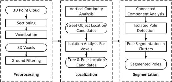
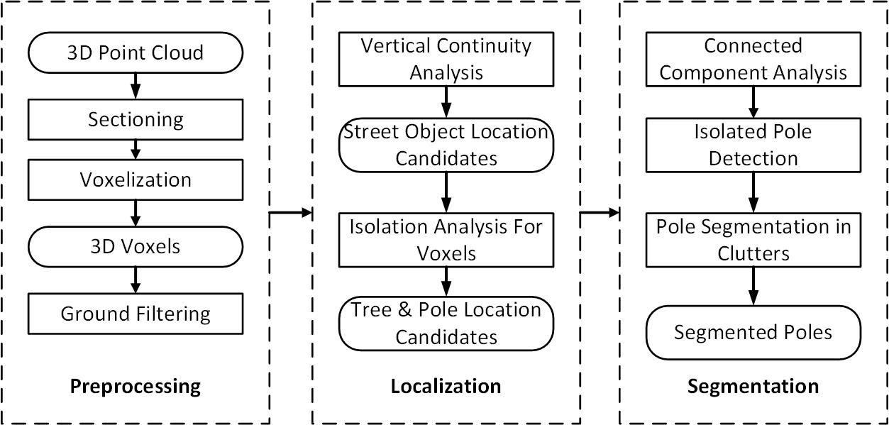
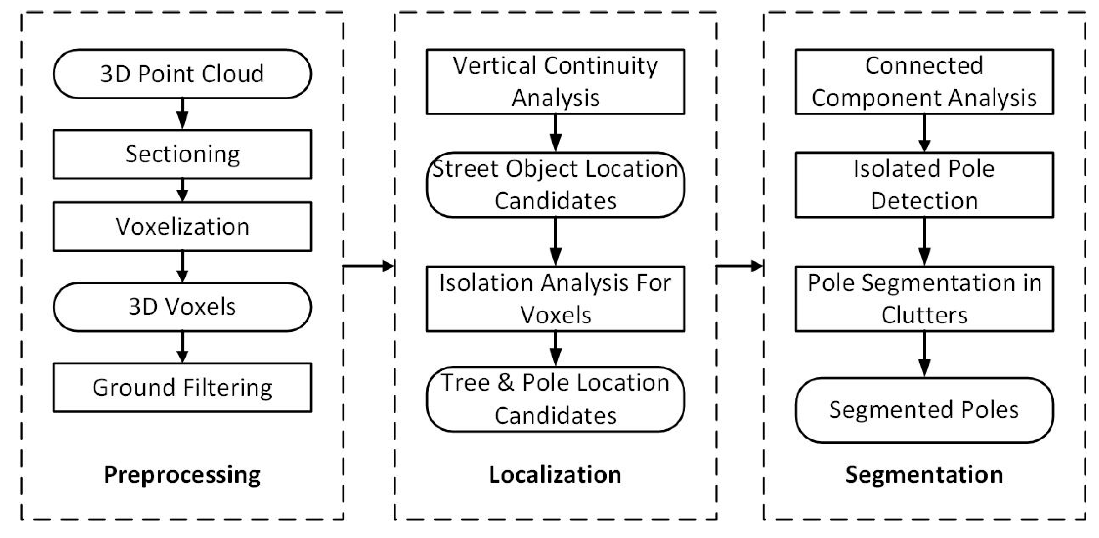
- (1)
- Pre-processing: Original unorganized MLS data are sectioned and reorganized based on voxels; then, the whole scene is classified as ground and non-ground voxels.
- (2)
- Localization: A voxel-based method utilizing isolation analysis to detect the position of poles, including trees.
- (3)
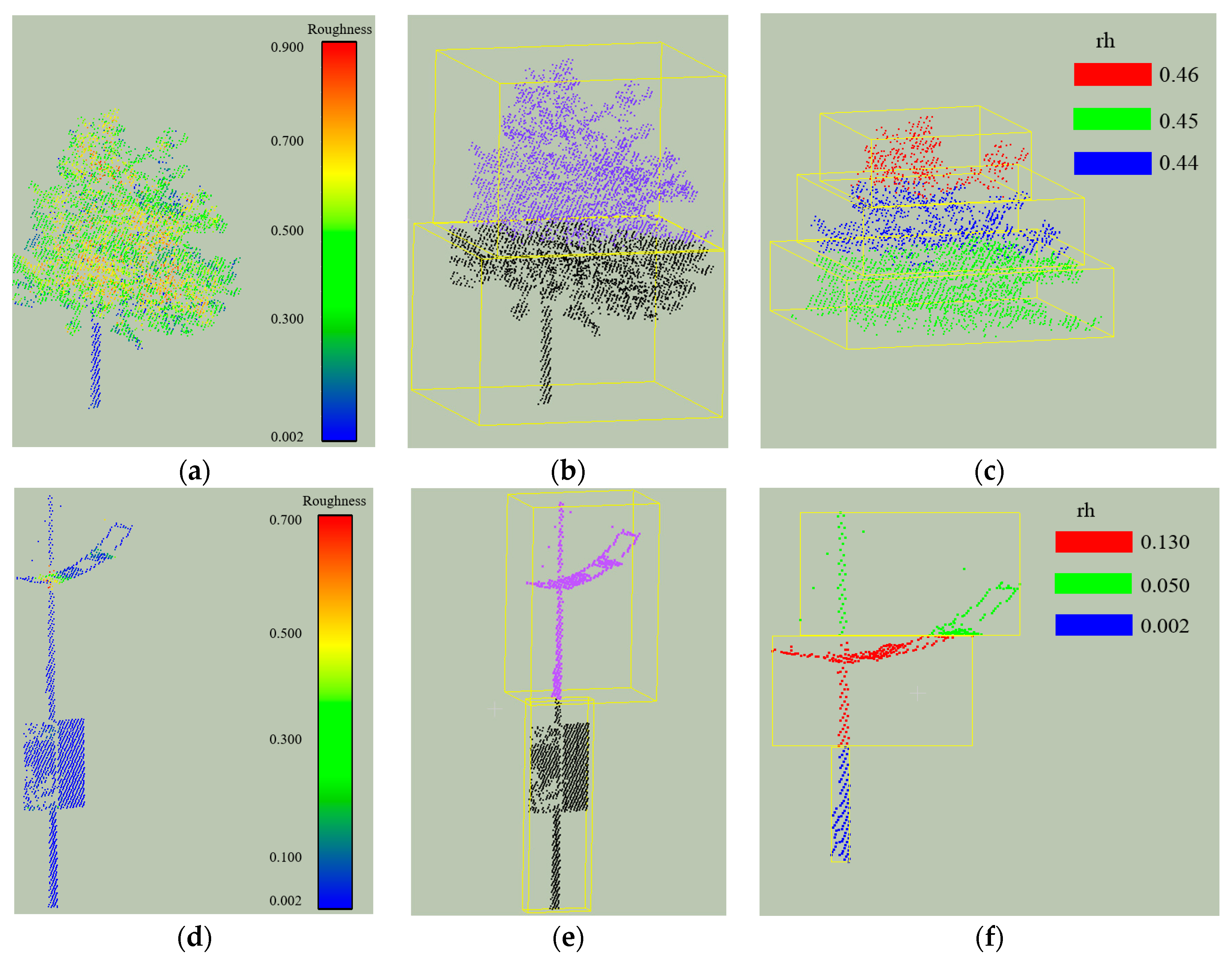
- Segmentation: Differentiate poles from trees using roughness analysis from isolated segments and segment poles from connected furniture segments by detecting man-made structures.
3.1. Pre-Processing of Original MLS Data
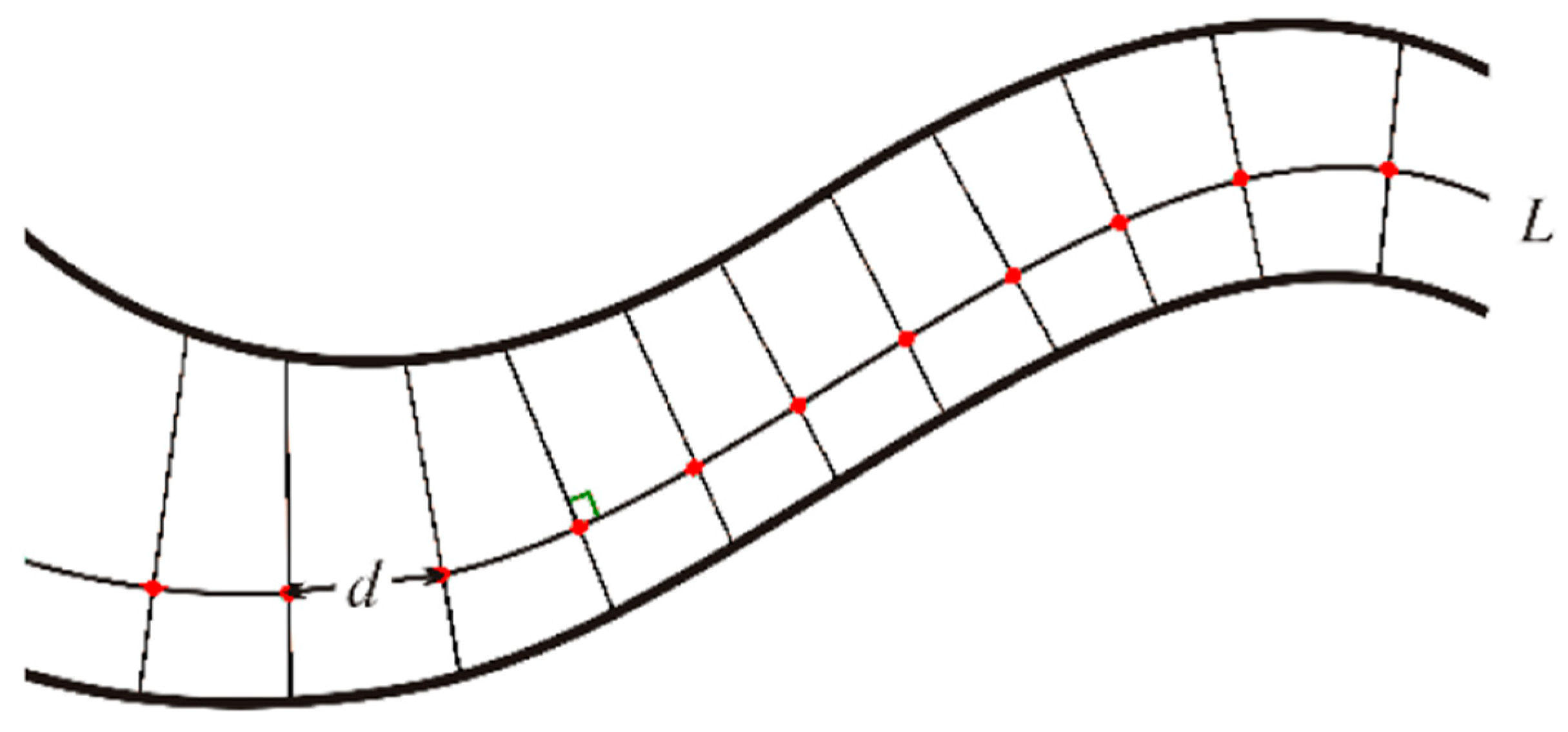
3.1.1. Sectioning of Original Data
3.1.2. Voxelization
3.1.3. Ground Detection
3.2. Localization of Poles and Trees
3.2.1. Localization of Street Objects
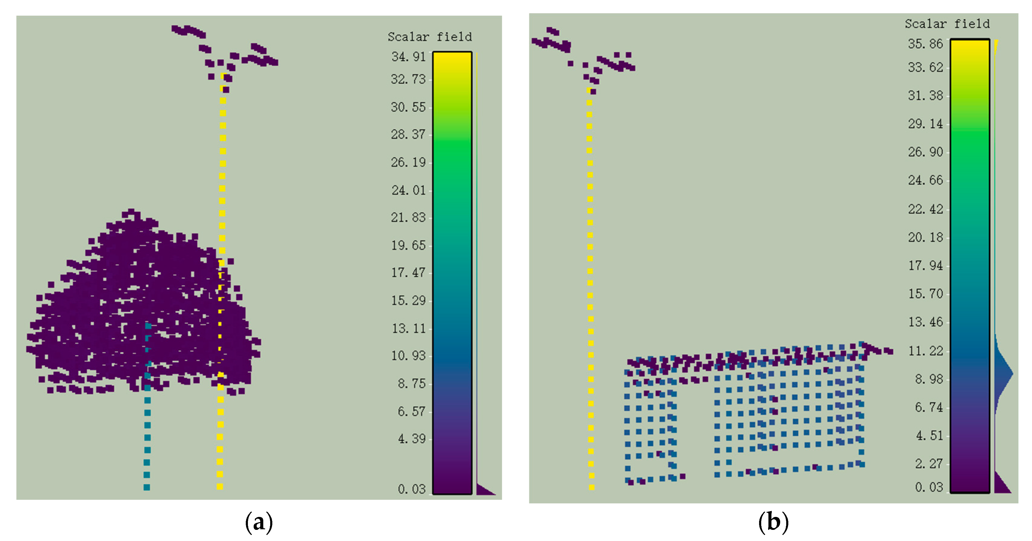
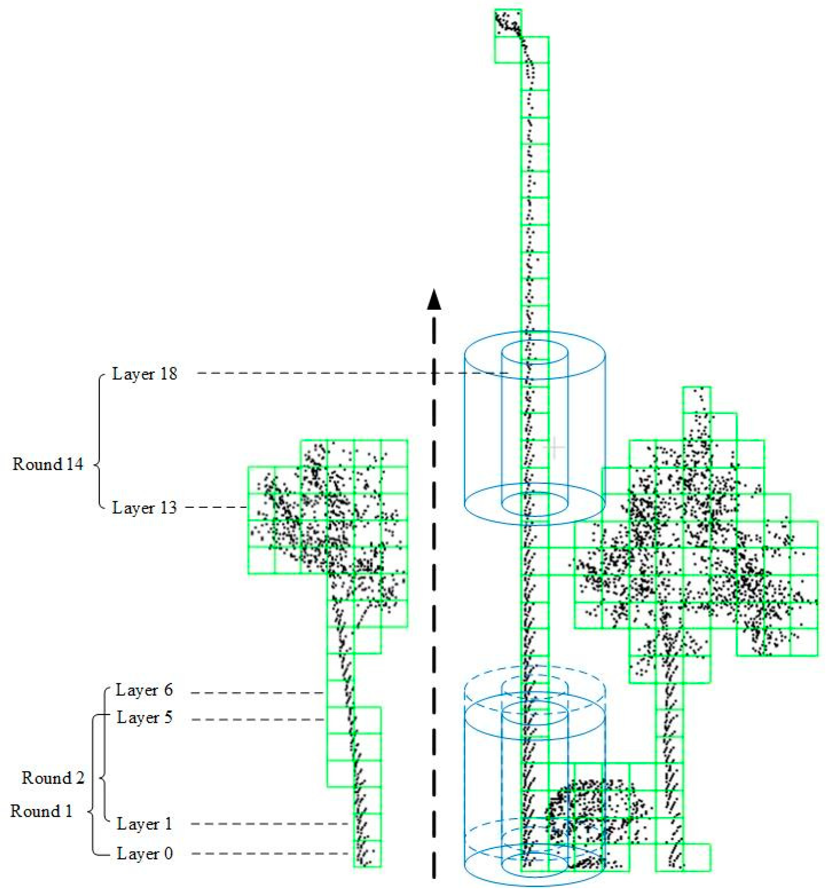
3.2.2. Selecting Candidate Locations of Road Poles and Trees
| Algorithm 1 Isolation analysis for voxels |
| Input: : one candidate object position S: a cluster v in Parameters: L: height of the cylinder N: allowed number of noise points in the ring between cylinders n: layer counter Ir: radius of the inner cylinder Or: radius of the outer cylinder Start: repeat (1) Select voxels V from layer n to layer n + L − 1 from S (2) Build a concentric cylinder with Ir as the inner cylinder radius and Or as the outer cylinder radius, selecting v as the centre, cylinder height starts from n and end at n + L − 1 (3) Count number of points np and number of voxels nv between two cylinders np (4) if np < NP && nv < NV (5) v is recognized as pole or tree position (6) break (7) else (8) n = n + 1 until all layers of S are reached |
3.3. Extraction of Road Poles
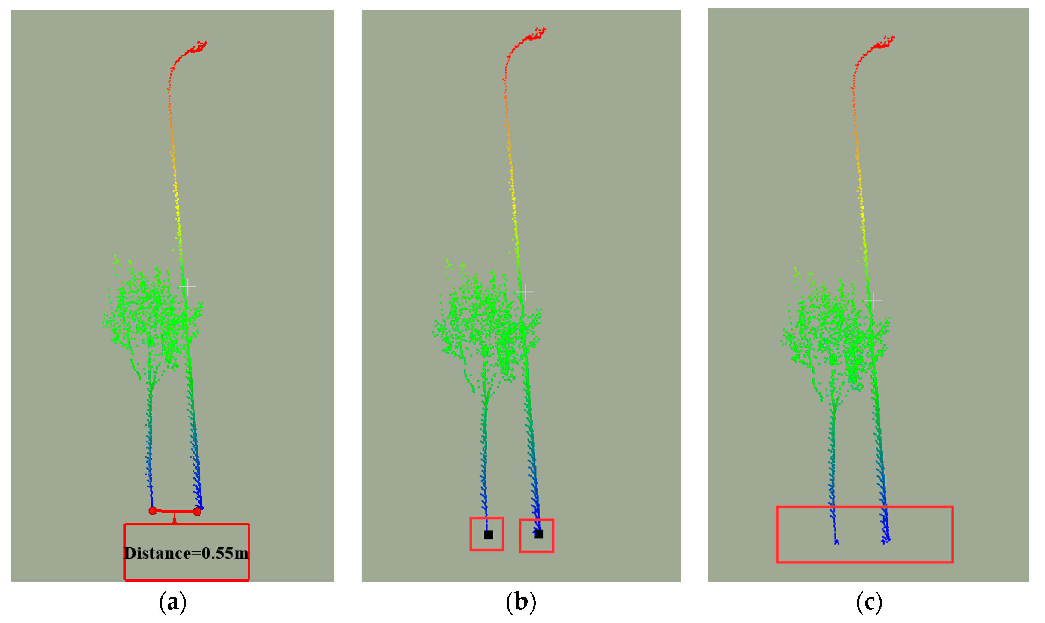
3.3.1. Detection of Isolated Poles
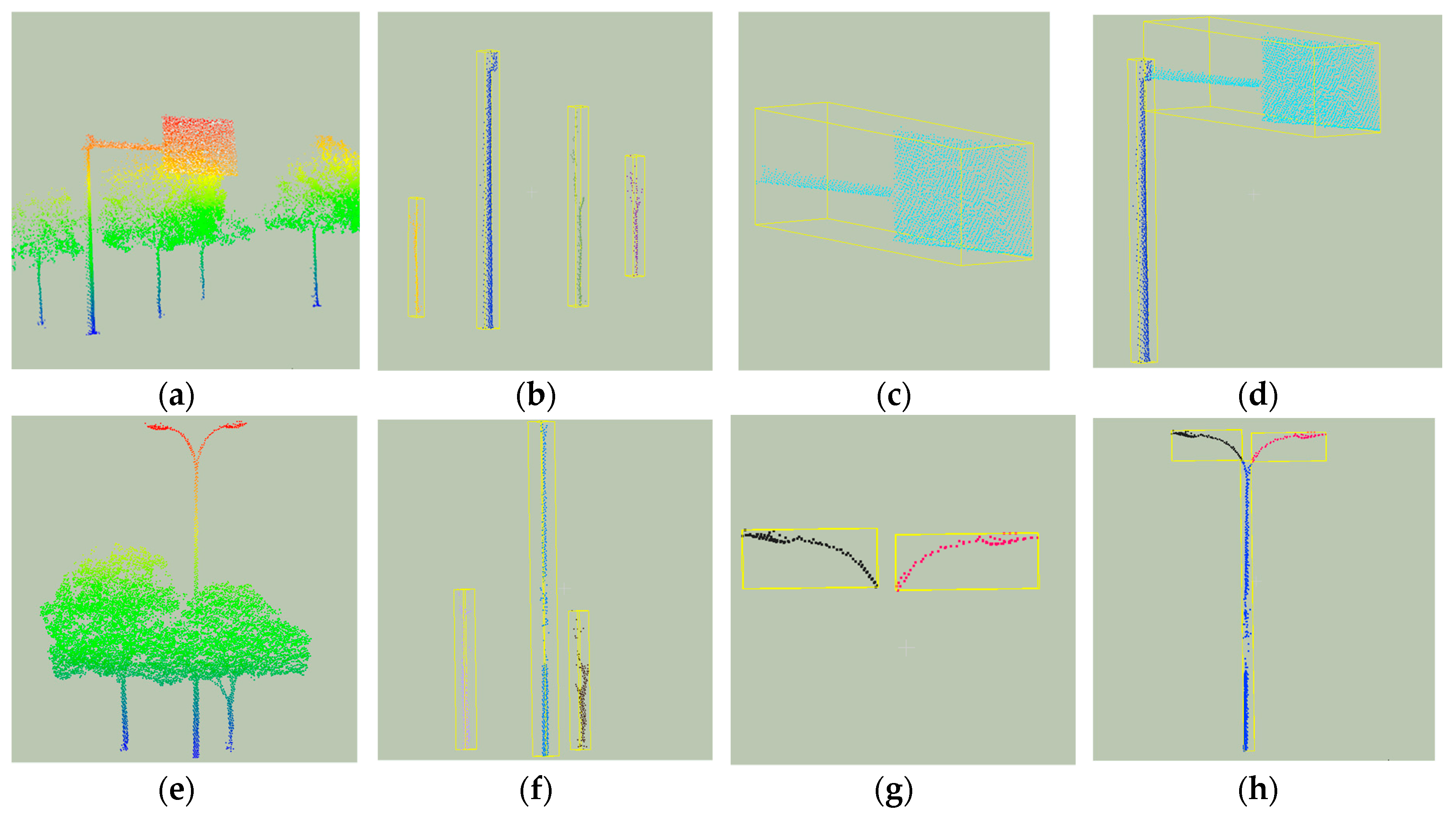
3.3.2. Detection of Poles in Clutters
Extracting Pole Part of a Pole in Clutters
| Algorithm 2 Vertical growing algorithm |
| Input: : one original seed on pole part of a pole S: point cloud cluster s locates on Parameters: r: radius of current MBC s: current seed Start: Initialize s = repeat (1) Find neighbouring points of s from S within radius 3r: N (2) Select points U from N: higher than the seed s & horizontal distance to s is less than 1.2r (3) Project U to the horizontal plane (4) Calculate the MBR of (5) Calculate the radius of MBC r, set the centre of the MBC as s until no points exist in the upper area U Output: P: pole part points |
Segmenting Poles in Clusters
| Algorithm 3 Region growing based on roughness |
| Input: P: point cloud cluster Parameters: : roughness threshold : roughness difference threshold : roughness values : point with minimum roughness value in S Start: Initialize with R = P = {} A = P Repeat (1) Current region =, current seeds = (2) Select point with minimum roughness value from A (3) ={}, {} (4) Delete from A (5) Repeat (6) Select one point in (7) Find neighbours of : (8) Repeat (9) Select one point in : : (10) If A contains and || < (11) Add to (12) Delete in A (13) If < : (14) Add to (15) Until all points in are traversed (16) Until all points in are traversed (17) Add current region to R Until no points exist C Output: R: manmade structure cluster |
4. Experiments
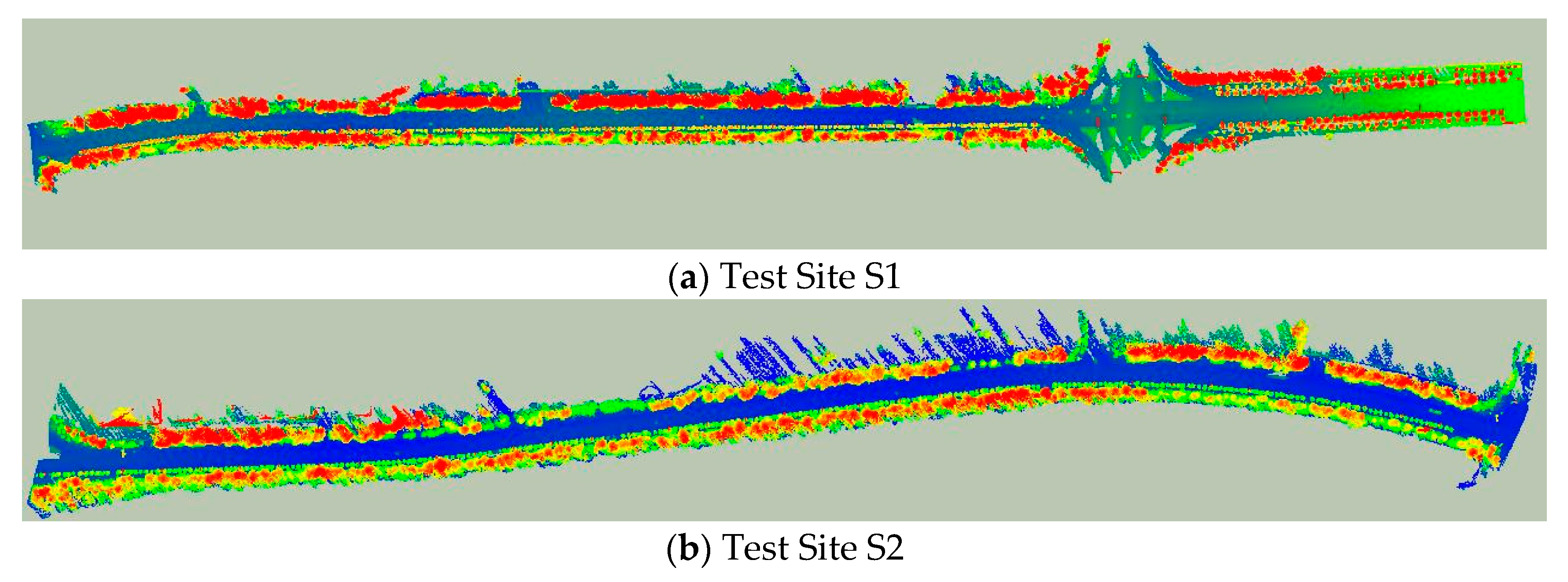
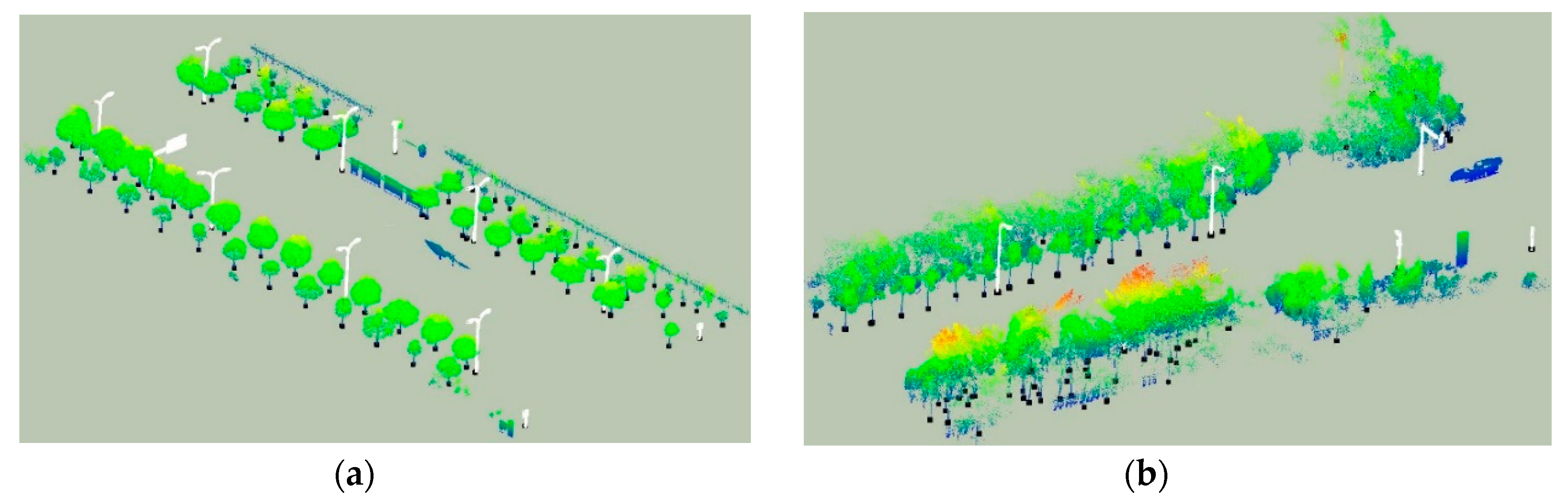
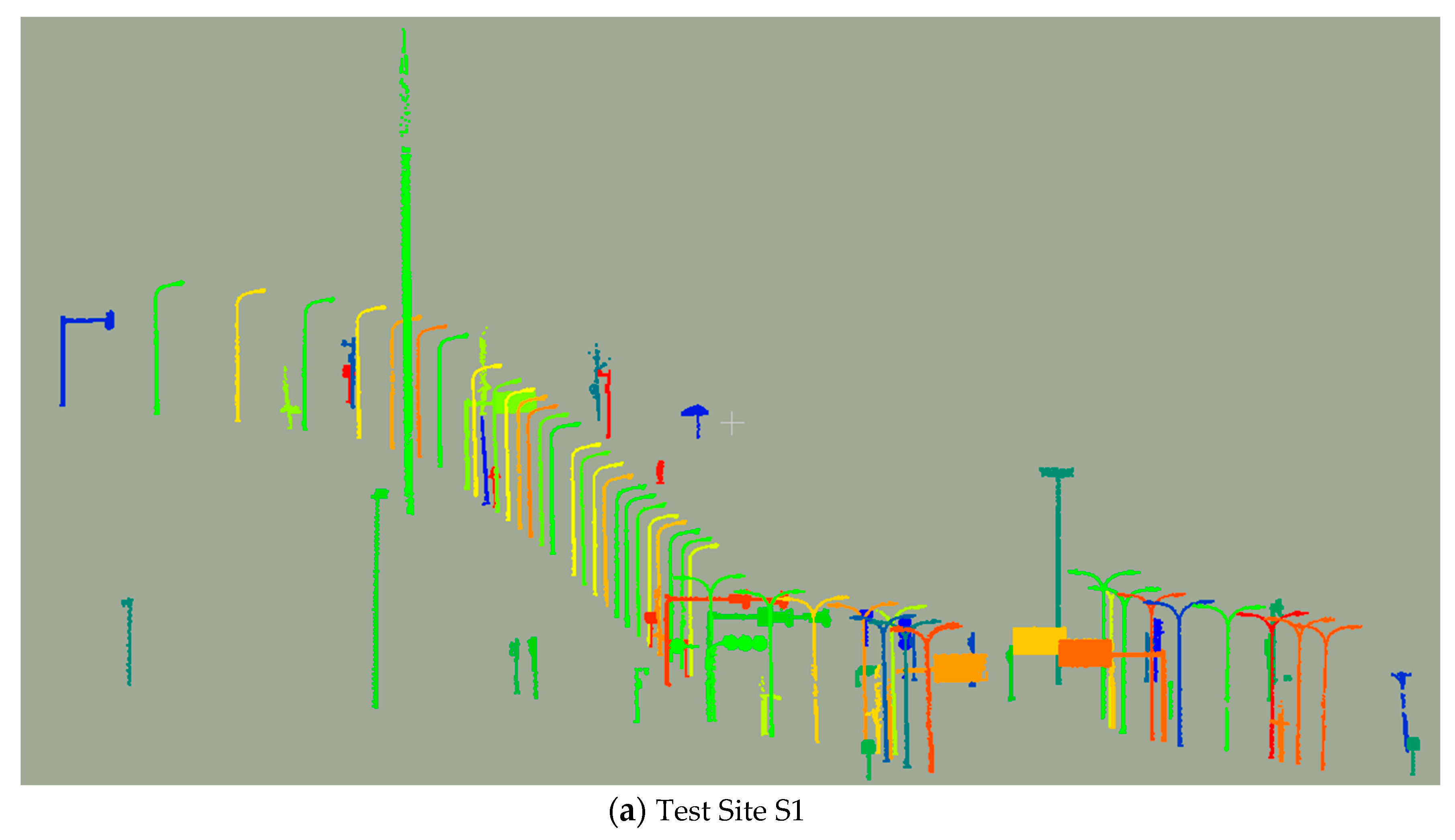
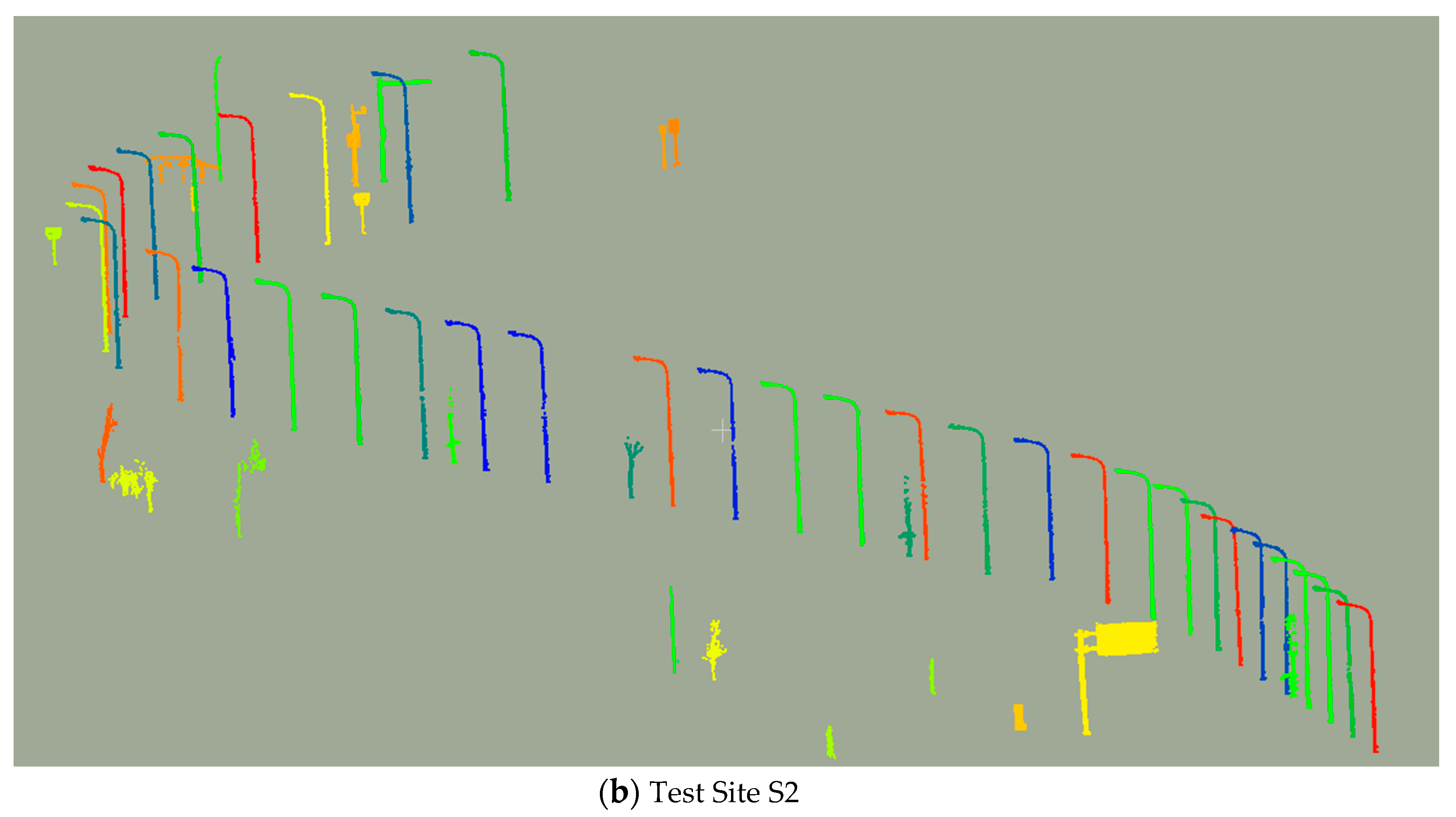
4.1. Test Sites
4.2. Parameter Settings
4.3. Results
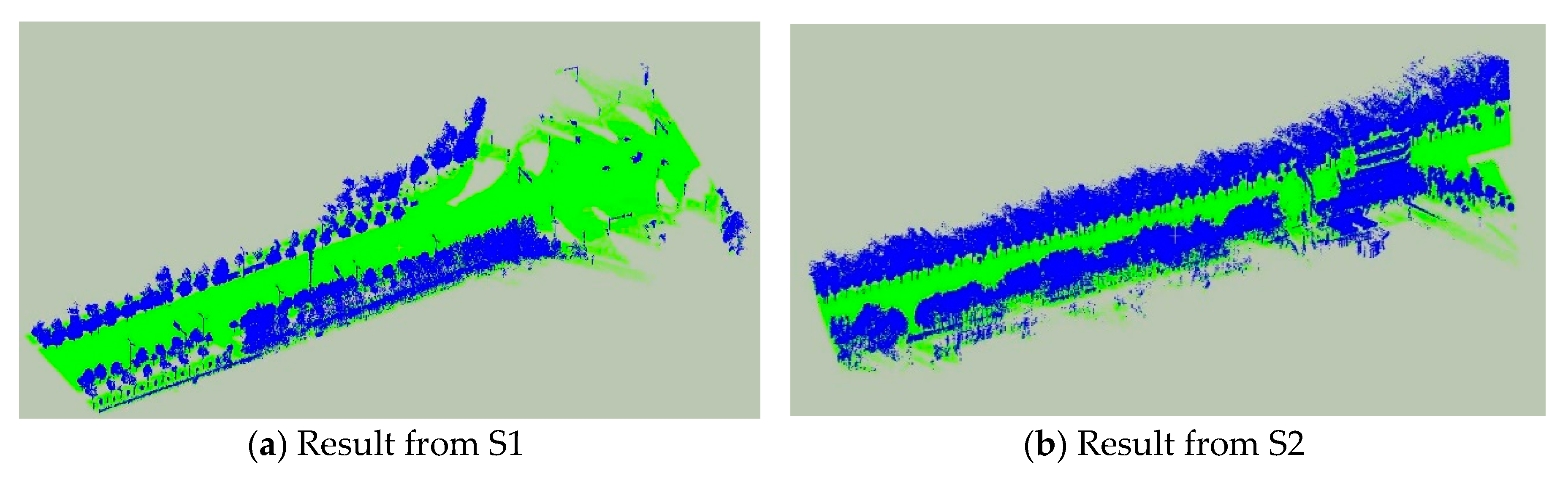
4.3.1. Pre-Processing Results
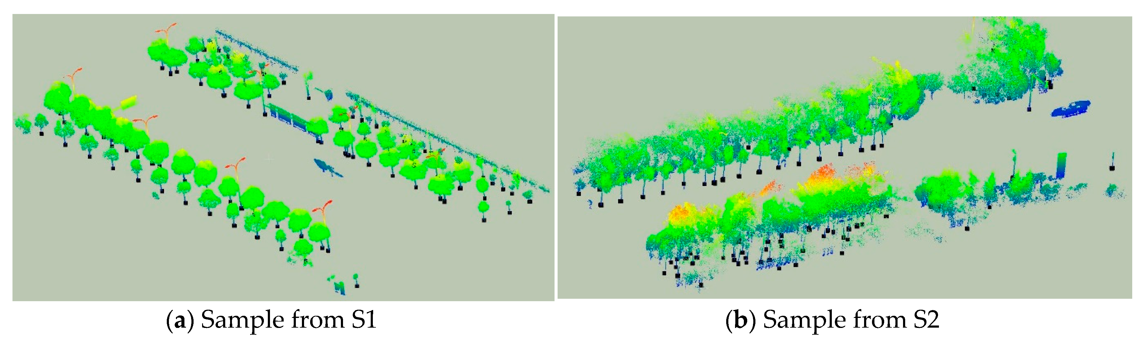
4.3.2. Results of Poles and Trees Localization
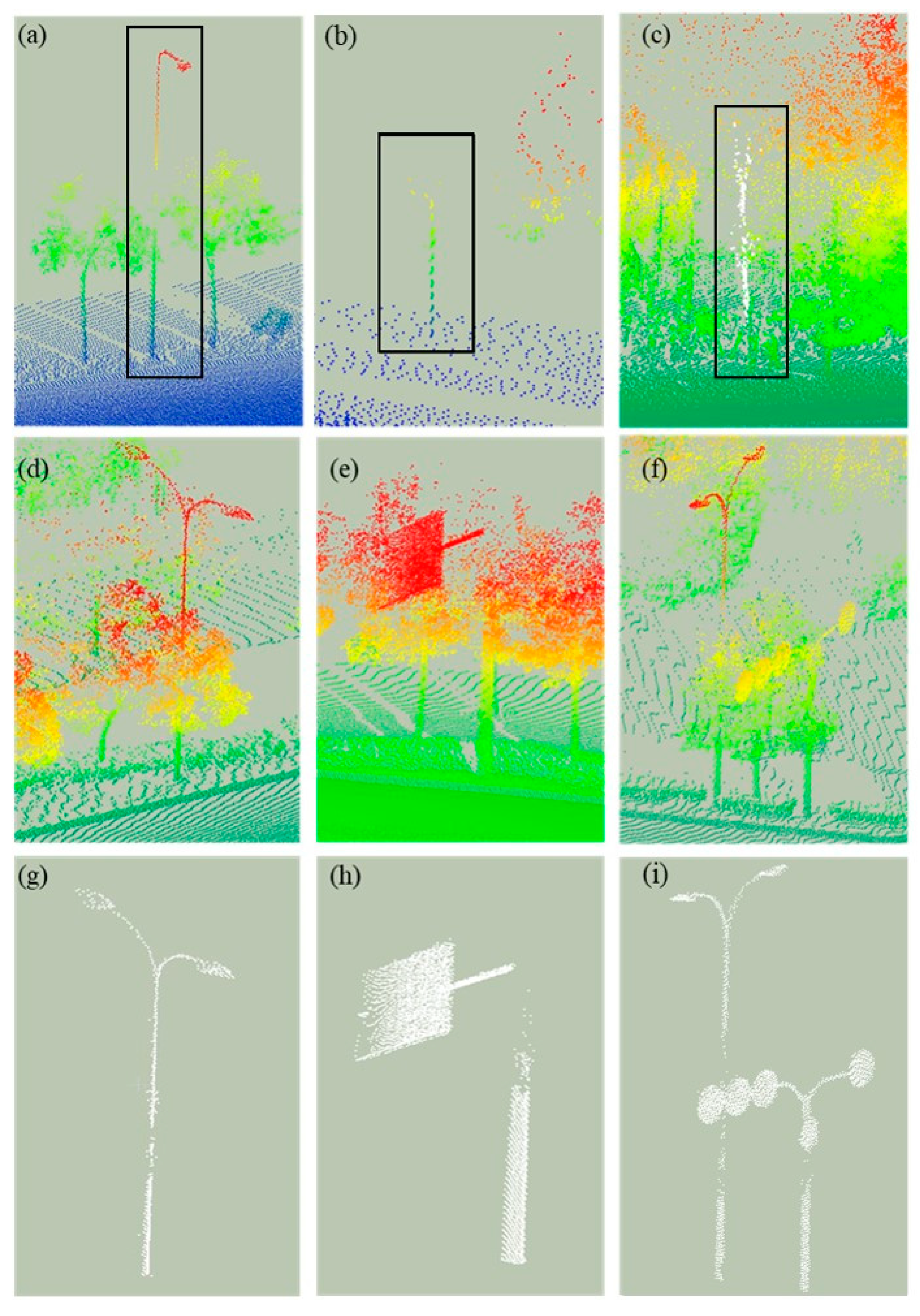
4.3.3. Pole Detection Results
4.4. Performance Analysis of the Algorithm
4.5. Comparison with Previous Methods
5. Conclusions
Author Contributions
Funding
Conflicts of Interest
References
- Pu, S.; Vosselman, G. Automatic extraction of building features from terrestrial laser scanning. Int. Arch. Photogramm. Remote Sens. Spatial Inf. Sci. 2006, 36, 25–27. [Google Scholar]
- Pu, S.; Rutzinger, M.; Vosselman, G.; Oude Elberink, S. Recognizing basic structures from mobile laser scanning data for road inventory studies. ISPRS J. Photogramm. Remote Sens. 2011, 66, S28–S39. [Google Scholar] [CrossRef]
- Li, L.; Li, Y.; Li, D. A method based on an adaptive radius cylinder model for detecting pole-like objects in mobile laser scanning data. Remote Sens. Lett. 2016, 7, 249–258. [Google Scholar] [CrossRef]
- Brenner, C. Extraction of Features from Mobile Laser Scanning Data for Future Driver Assistance Systems. Lect. Notes Geoinf. Cartogr. 2009. [Google Scholar] [CrossRef]
- Brenner, C. Global localization of vehicles using local pole patterns. In Pattern Recognition; Springer: Berlin, Germany, 2009; pp. 61–70. [Google Scholar]
- Lehtomäki, M.; Jaakkola, A.; Hyyppä, J.; Lampinen, J.; Kaartinen, H.; Kukko, A.; Puttonen, E.; Hyyppä, H. Object classification and recognition from mobile laser scanning point clouds in a road environment. IEEE Trans. Geosci. Remote Sens. 2016, 54, 1226–1239. [Google Scholar] [CrossRef]
- Liang, X.; Litkey, P.; Hyyppa, J.; Kaartinen, H.; Vastaranta, M.; Holopainen, M. Automatic Stem Mapping Using Single-Scan Terrestrial Laser Scanning. IEEE Trans. Geosci. Remote Sens. 2012, 50, 661–670. [Google Scholar] [CrossRef]
- Huang, P.; Cheng, M.; Chen, Y.; Luo, H.; Wang, C.; Li, J. Traffic Sign Occlusion Detection Using Mobile Laser Scanning Point Clouds. IEEE Trans. Intell. Transp. Syst. 2017, 1–13. [Google Scholar] [CrossRef]
- Raumonen, P.; Kaasalainen, M.; Åkerblom, M.; Kaasalainen, S.; Kaartinen, H.; Vastaranta, M.; Holopainen, M.; Disney, M.; Lewis, P. Fast Automatic Precision Tree Models from Terrestrial Laser Scanner Data. Remote Sens. 2013, 5, 491–520. [Google Scholar] [CrossRef] [Green Version]
- Elberink, S.O.; Khoshelham, K. Automatic Extraction of Railroad Centerlines from Mobile Laser Scanning Data. Remote Sens. 2015, 7, 5565–5583. [Google Scholar] [CrossRef] [Green Version]
- Jochem, A.; Höfle, B.; Rutzinger, M. Extraction of Vertical Walls from Mobile Laser Scanning Data for Solar Potential Assessment. Remote Sens. 2011, 3, 650–667. [Google Scholar] [CrossRef]
- Kaasalainen, S.; Jaakkola, A.; Kaasalainen, M.; Krooks, A.; Kukko, A. Analysis of incidence angle and distance effects on terrestrial laser scanner intensity: Search for correction methods. Remote Sens. 2011, 3, 2207–2221. [Google Scholar] [CrossRef]
- Lehtomäki, M.; Jaakkola, A.; Hyyppä, J.; Kukko, A.; Kaartinen, H. Detection of Vertical Pole-Like Objects in a Road Environment Using Vehicle-Based Laser Scanning Data. Remote Sens. 2010, 2, 641–664. [Google Scholar] [CrossRef] [Green Version]
- Yokoyama, H.; Date, H.; Kanai, S.; Takeda, H. Detection and Classification of Pole-like Objects from Mobile Laser Scanning Data of Urban Environments. Int. J. CAD/CAM 2013, 13, 31–40. [Google Scholar]
- Yang, B.; Zhen, D. A shape based segmentation method for mobile laser scanning point clouds. ISPRS J. Photogramm. Remote Sens. 2013, 81, 19–30. [Google Scholar] [CrossRef]
- Yang, B.; Dong, Z.; Zhao, G.; Dai, W. Hierarchical extraction of urban objects from mobile laser scanning data. ISPRS J. Photogramm. Remote Sens. 2015, 99, 45–57. [Google Scholar] [CrossRef]
- Wu, B.; Yu, B.; Yue, W.; Shu, S.; Tan, W.; Hu, C.; Huang, Y.; Wu, J.; Liu, H. A Voxel-Based Method for Automated Identification and Morphological Parameters Estimation of Individual Street Trees from Mobile Laser Scanning Data. Remote Sens. 2013, 5, 584–611. [Google Scholar] [CrossRef] [Green Version]
- Rodríguez-Cuenca, B.; García-Cortés, S.; Ordóñez, C.; Alonso, M. Automatic Detection and Classification of Pole-Like Objects in Urban Point Cloud Data Using an Anomaly Detection Algorithm. Remote Sens. 2015, 7, 12680–12703. [Google Scholar] [CrossRef] [Green Version]
- Zhang, C.; Zhou, Y.; Qiu, F. Individual Tree Segmentation from LiDAR Point Clouds for Urban Forest Inventory. Remote Sens. 2015, 7, 7892–7913. [Google Scholar] [CrossRef] [Green Version]
- Li, F.; Elberink, S.O.; Vosselman, G. Pole-Like Street Furniture Decompostion in Mobile Laser Scanning Data. ISPRS Ann. Photogramm. Remote Sens. Spat. Inf. Sci. 2016, 3, 193–200. [Google Scholar] [CrossRef]
- Li, F.; Oude Elberink, S.; Vosselman, G. Pole-Like Road Furniture Detection and Decomposition in Mobile Laser Scanning Data Based on Spatial Relations. Remote Sens. 2018, 10, 531. [Google Scholar] [Green Version]
- Li, F.; Elberink, S.O.; Vosselman, G. Semantic labelling of road furniture in mobile laser scanning data. Int. Arch. Photogramm. Remote Sens. Spat. Inf. Sci. 2017, 42, 247–254. [Google Scholar] [CrossRef]
- Cabo, C.; Ordóñez, C.; García-Cortés, S.; Martínez, J. An algorithm for automatic detection of pole-like street furniture objects from Mobile Laser Scanner point clouds. ISPRS J. Photogramm. Remote Sens. 2014, 87, 47–56. [Google Scholar] [CrossRef]
- El-Halawanya, S.I.; Lichtia, D.D. Detecting road poles from mobile terrestrial laser scanning data. GISci. Remote Sens. 2013, 50, 704–722. [Google Scholar] [CrossRef]
- Golovinskiy, A.; Kim, V.G.; Funkhouser, T. Shape-based Recognition of 3D Point Clouds in Urban Environments. In Proceedings of the International Conference on Computer Vision (ICCV), Kyoto, Japan, 29 September–2 October 2009; pp. 2154–2161. [Google Scholar]
- Lai, K.; Fox, D. Object Recognition in 3D Point Clouds Using Web Data and Domain Adaptation. Int. J. Robot. Res. 2010, 29, 1019–1037. [Google Scholar] [CrossRef] [Green Version]
- Ishikawa, K.; Tonomura, F.; Amano, Y.; Hashizume, T. Recognition of Road Objects from 3D Mobile Mapping Data. Int. J. CAD/CAM 2013, 13, 41–48. [Google Scholar]
- Wang, J.; Lindenbergh, R.; Menenti, M. SigVox—A 3D feature matching algorithm for automatic street object recognition in mobile laser scanning point clouds. ISPRS J. Photogramm. Remote Sens. 2017, 128, 111–129. [Google Scholar] [CrossRef]
- Oude Elberink, S.; Kemboi, B. User-assisted object detection by segment based similarity measures in mobile laser scanner data. ISPRS-Int. Arch. Photogramm. Remote Sens. Spat. Inf. Sci. 2014, 3, 239–246. [Google Scholar] [CrossRef]
- Zhou, Y.; Wang, D.; Xie, X.; Ren, Y.; Li, G.; Deng, Y.; Wang, Z. A Fast and Accurate Segmentation Method for Ordered LiDAR Point Cloud of Large-Scale Scenes. IEEE Geosci. Remote Sens. Lett. 2014, 11, 1981–1985. [Google Scholar] [CrossRef]
- Wu, F.; Wen, C.; Guo, Y.; Wang, J.; Yu, Y.; Wang, C.; Li, J. Rapid Localization and Extraction of Street Light Poles in Mobile LiDAR Point Clouds: A Supervoxel-Based Approach. IEEE Trans. Intell. Transp. Syst. 2017, 18, 292–305. [Google Scholar] [CrossRef]
- Golovinskiy, A.; Funkhouser, T. Min-cut based segmentation of point clouds. In Proceedings of the IEEE 12th International Conference on Computer Vision Workshops (ICCV Workshops), Kyoto, Japan, 27 September–4 October 2009; pp. 39–46. [Google Scholar]
- Yu, Y.; Li, J.; Guan, H.; Wang, C.; Yu, J. Semiautomated Extraction of Street Light Poles from Mobile LiDAR Point-Clouds. IEEE Trans. Geosci. Remote Sens. 2015, 53, 1374–1386. [Google Scholar] [CrossRef]
- Li, Y.; Li, L.; Li, D.; Yang, F.; Liu, Y. A Density-Based Clustering Method for Urban Scene Mobile Laser Scanning Data Segmentation. Remote Sens. 2017, 9, 331. [Google Scholar] [CrossRef]
- Toth, C.; Paska, E.; Brzezinska, D. Using road pavement markings as ground control for lidar data. Int. Arch. Photogramm. Remote Sens. Spat. Inf. Sci. 2008, 37, 189–195. [Google Scholar]
- Yang, B.; Fang, L.; Li, Q.; Li, J. Automated extraction of road markings from mobile lidar point clouds. Photogramm. Eng. Remote Sens. 2012, 78, 331–338. [Google Scholar] [CrossRef]
- Yang, B.; Fang, L.; Li, J. Semi-automated extraction and delineation of 3D roads of street scene from mobile laser scanning point clouds. ISPRS J. Photogramm. Remote Sens. 2013, 79, 80–93. [Google Scholar] [CrossRef]
- Guan, H.; Li, J.; Yu, Y.; Wang, C.; Chapman, M.; Yang, B. Using mobile laser scanning data for automated extraction of road markings. ISPRS J. Photogramm. Remote Sens. 2014, 87, 93–107. [Google Scholar] [CrossRef]
- Kumar, P.; McElhinney, C.P.; Lewis, P.; McCarthy, T. An automated algorithm for extracting road edges from terrestrial mobile LiDAR data. ISPRS J. Photogramm. Remote Sens. 2013, 85, 44–55. [Google Scholar] [CrossRef] [Green Version]
- Chen, D.; He, X. Fast automatic three-dimensional road model reconstruction based on mobile laser scanning system. Opt.-Int. J. Light Electron Opt. 2015, 126, 725–730. [Google Scholar] [CrossRef]
- Riveiro, B.; González-Jorge, H.; Martínez-Sánchez, J.; Díaz-Vilariño, L.; Arias, P. Automatic detection of zebra crossings from mobile LiDAR data. Opt. Laser Technol. 2015, 70, 63–70. [Google Scholar] [CrossRef]
- Rodríguez-Cuenca, B.; García-Cortés, S.; Ordóñez, C.; Alonso, M.C. An approach to detect and delineate street curbs from MLS 3D point cloud data. Autom. Constr. 2015, 51, 103–112. [Google Scholar] [CrossRef]
- Ordóñez, C.; Cabo, C.; Sanz-Ablanedo, E. Automatic Detection and Classification of Pole-Like Objects for Urban Cartography Using Mobile Laser Scanning Data. Sensors 2017, 17, 1465. [Google Scholar] [CrossRef]
- Demantké, J.; Mallet, C.; David, N.; Vallet, B. Dimensionality based scale selection in 3D lidar point clouds. Int. Arch. Photogramm. Remote Sens. Spat. Inf. Sci. 2012, 3812, 97–102. [Google Scholar]
- Li, L.; Li, D.; Zhu, H.; Li, Y. A dual growing method for the automatic extraction of individual trees from mobile laser scanning data. ISPRS J. Photogramm. Remote Sens. 2016, 120, 37–52. [Google Scholar] [CrossRef]
- Li, L.; Zhang, D.; Ying, S.; Li, Y. Recognition and Reconstruction of Zebra Crossings on Roads from Mobile Laser Scanning Data. ISPRS Int. J. Geo-Inf. 2016, 5, 125. [Google Scholar] [CrossRef]


| Test Sites | Length (m) | Width (m) | Points (million) | Average Density (points/m2) |
|---|---|---|---|---|
| S1 | 1400 | 60 | 23.6 | 445 |
| S2 | 1200 | 50 | 20.7 | 345 |
| Name | Values | Description |
|---|---|---|
| VS | 0.3 m | Voxel size |
| Ir | 1.5 (0.45 m) | Inner radius |
| Or | 3 (0.9 m) | Outer radius |
| NP | 4 | Number of points allowed in the ring of the concentric cylinder |
| NV | 1 | Number of voxels allowed in the ring of the concentric cylinder |
| L | 4 (1.2 m) | The height of the cylinder |
| 0.07 | The threshold value of roughness that separate tree crowns from poles |
| Test Sites | Lamp Posts | Traffic Signs | Traffic Lights | Other Poles | Completeness | Correctness |
|---|---|---|---|---|---|---|
| S1 | 45/47 | 15/15 | 12/13 | 12/13 | 82/86 (95.3%) | 82/91 (90.1%) |
| S2 | 36/37 | 6/6 | 1/1 | 2/3 | 45/47 (95.7%) | 45/61 (73.8%) |
| Average | 95.5% | 83.6% | ||||
© 2019 by the authors. Licensee MDPI, Basel, Switzerland. This article is an open access article distributed under the terms and conditions of the Creative Commons Attribution (CC BY) license (http://creativecommons.org/licenses/by/4.0/).
Share and Cite
Li, Y.; Wang, W.; Tang, S.; Li, D.; Wang, Y.; Yuan, Z.; Guo, R.; Li, X.; Xiu, W. Localization and Extraction of Road Poles in Urban Areas from Mobile Laser Scanning Data. Remote Sens. 2019, 11, 401. https://0-doi-org.brum.beds.ac.uk/10.3390/rs11040401
Li Y, Wang W, Tang S, Li D, Wang Y, Yuan Z, Guo R, Li X, Xiu W. Localization and Extraction of Road Poles in Urban Areas from Mobile Laser Scanning Data. Remote Sensing. 2019; 11(4):401. https://0-doi-org.brum.beds.ac.uk/10.3390/rs11040401
Chicago/Turabian StyleLi, You, Weixi Wang, Shengjun Tang, Dalin Li, Yankun Wang, Zhilu Yuan, Renzhong Guo, Xiaoming Li, and Wenqun Xiu. 2019. "Localization and Extraction of Road Poles in Urban Areas from Mobile Laser Scanning Data" Remote Sensing 11, no. 4: 401. https://0-doi-org.brum.beds.ac.uk/10.3390/rs11040401