Article

Co- and post-seismic Deformation Mechanisms of the MW 7.3 Iran Earthquake (2017) Revealed by Sentinel-1 InSAR Observations

1
College of Geology Engineering and Geomatics, Chang’an University, Xi’an 710054, China
2
China Institute of Geo-Environment Monitoring, Beijing 100081, China
*
Authors to whom correspondence should be addressed.
Submission received: 28 December 2018 / Revised: 1 February 2019 / Accepted: 14 February 2019 / Published: 18 February 2019
(This article belongs to the Special Issue Remote Sensing of Tectonic Deformation)

Abstract

:
The extraction of high-accuracy co- and post-seismic deformation fields and inversions of seismic slip distributions is significant in the comprehension of seismogenic mechanisms. On 12 November 2017, a MW 7.3 earthquake occurred on the border between Iran and Iraq. To construct the co-seismic deformation field, Sentinel-1A synthetic aperture radar (SAR) images from three tracks were used. Based on a prior knowledge, least-squares iterative approximation was employed to construct the three-dimensional (3D) co-seismic deformation field. to derive a time series of 2D post-seismic deformation, the multidimensional small baseline subset (MSBAS) technique was use. Co-seismic deformation fields were asymmetric; the maximum relative displacement was nearly 90cm in the radar line-of-sight between two centers of co-seismic deformation. The 3D co-seismic deformation field showed southwestward horizontal motion and continuous subsidence-to-uplift variation from northeast to southwest. The two-dimensional (2D) post-seismic deformation time series showed a gradual decaying trend and good correspondence with the aftershock distribution. The main mechanism of post-seismic deformation was an afterslip of the post-seismic faults. We used the elastic half-space model to invert co-seismic deformation fields and obtain source parameters of the slip model. The maximum and average slips were 2.5 and 0.72 m, respectively. The average slip angle was 126.38° and the moment magnitude was MW 7.34. The results of this study will contribute to research on regional tectonic activities.

Graphical Abstract

1. Introduction

At 18:18 UTC on 12 November 2017, a MW 7.3 earthquake occurred at the border between Sulaymaniyah Province, Iraq and the Kermanshah Province, Iran (Figure 1; hereafter referred to as the Iran earthquake). This event killed more than 400 people and injured over 8000; more than 12,000 buildings were destroyed and there were serious economic losses [1]. Surface deformation is the most direct apparent phenomenon of earthquakes and it provides important information for studying the damage and fault structure. Interferometric synthetic aperture radar (InSAR) is a type of remote sensing geodetic technique that provides many advantages, including high spatial resolution, high precision, and continuous coverage over a wide area [2,3]. InSAR is an important tool for mapping earthquake-induced ground deformation and estimating source parameters [4,5,6].
After the Iran earthquake, many researchers used InSAR technology to study the co-seismic surface displacement and seismological structure. Kobayashi et al. [7] used ALOS-2 data to acquire the co-seismic line-of-sight (LOS) deformation field and inverted the source parameters. Through the use of ALOS-2 and Sentinel-1A data, Wang et al. [8] retrieved the three-dimensional (3D) co-seismic deformation fields. Feng et al. [9] derived the post-seismic surface deformation in the first month after the mainshock from Sentinel-1A data. Different researchers have presented solutions for the focal mechanism, as listed in Table 1 [9,10,11]. Although previous studies have monitored co-seismic deformation and inverted the co-seismic source parameters, they have significant differences in whether there are one or two slip centers in the earthquake.
Post-seismic deformation carries key information in understanding stress increases that are induced by the mainshock and the mechanism of aftershock triggering. However, few studies have focused on the post-seismic deformation and the relationship between the mainshock and aftershocks. In order to understand the focal mechanism of the Iran earthquake and to analyze post-seismic deformation characteristics, we collected Sentinel-1A data in both the ascending and descending modes within 220 days after the mainshock. First, the co-seismic deformation field was constructed using the differential interferometry synthetic aperture radar (D-InSAR) [12,13]. Second, to construct 3D co-seismic deformation fields, we used the least-squares iterative approximation algorithm based on a prior knowledge (hereafter referred to as the indirect solution) [14]. Third, we inverted the source geometries based on a Bayesian inversion and performed a linear inversion to retrieve the slip distribution [15]. Finally, a two-dimensional (2D) time series of the post-seismic deformation was constructed using the multidimensional small baseline subset (MSBAS) [16] technique, and the temporal evolution of the afterslip was compared with the aftershocks to examine the regional tectonic movement.

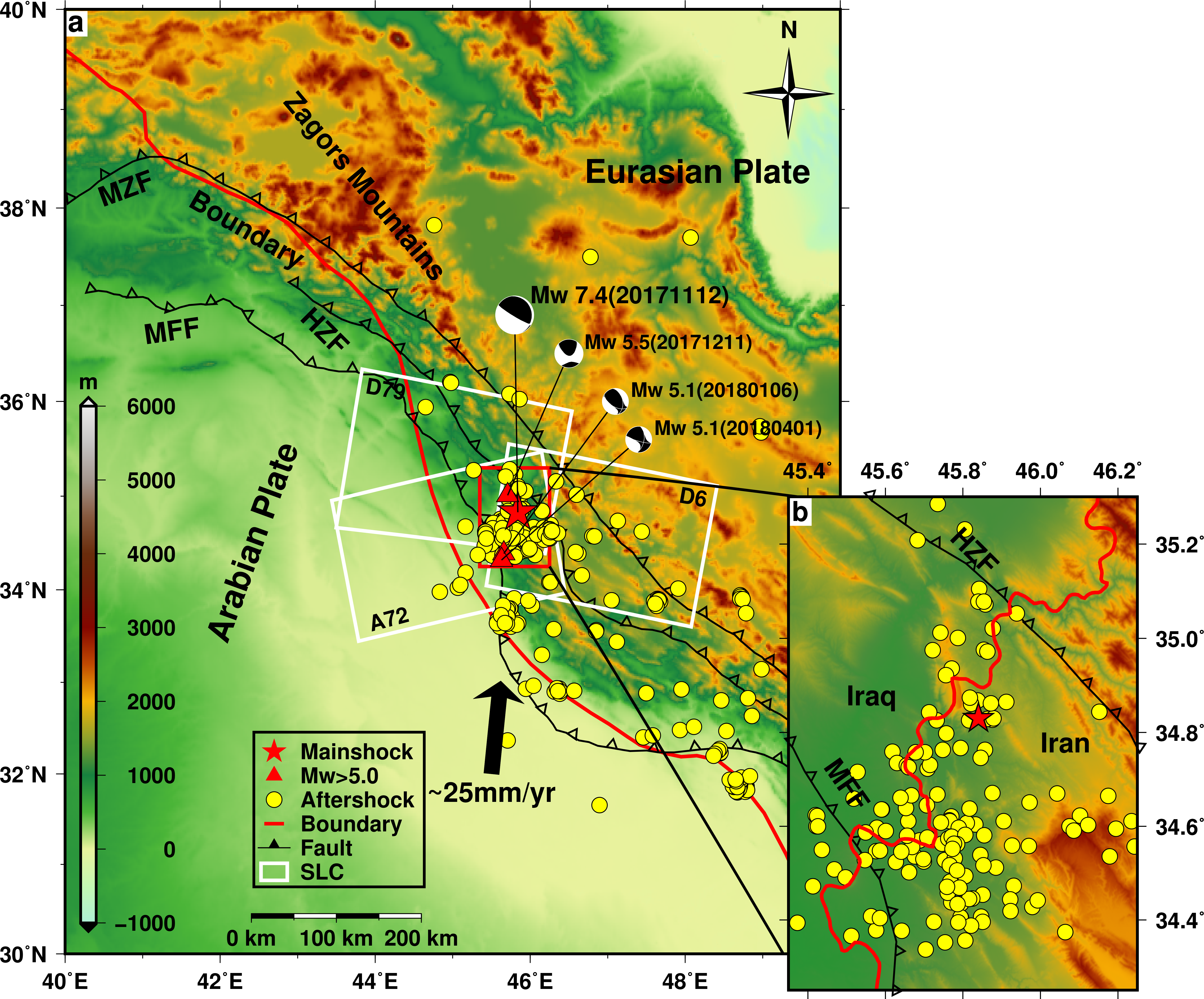
2. Geological Background

The Iran earthquake took place in the northwest Zagros fold-thrust belt, which has a series of fault structures that are dominated by an overthrust structure. As shown in Figure 1, the area has three main faults: the main Zagros Thrust Fault (MZF), the High Zagros Fault (HZF), and the Zagros Mountain Front Fault (MFF). This region of the Zagros Mountains formed due to the collision of the Arabian Plate with the Eurasian Plate; the Arabian Plate is moving towards the Eurasian Plate at an average convergence rate of 20–25 mm/year. It is one of the most seismically active intra-continental fold-and-thrust belts on Earth. Reverse and strike-slip faults partition the compressional structures in this range [17,18,19]. Yang et al. [20] demonstrated the future potential for earthquakes with larger magnitudes. Therefore, an in-depth study on the co- and post-seismic deformation characteristics of the Iran earthquake have great significance for clarifying the geometry and kinematics of structures in this region and assessing future seismic trends.

3. Methodology

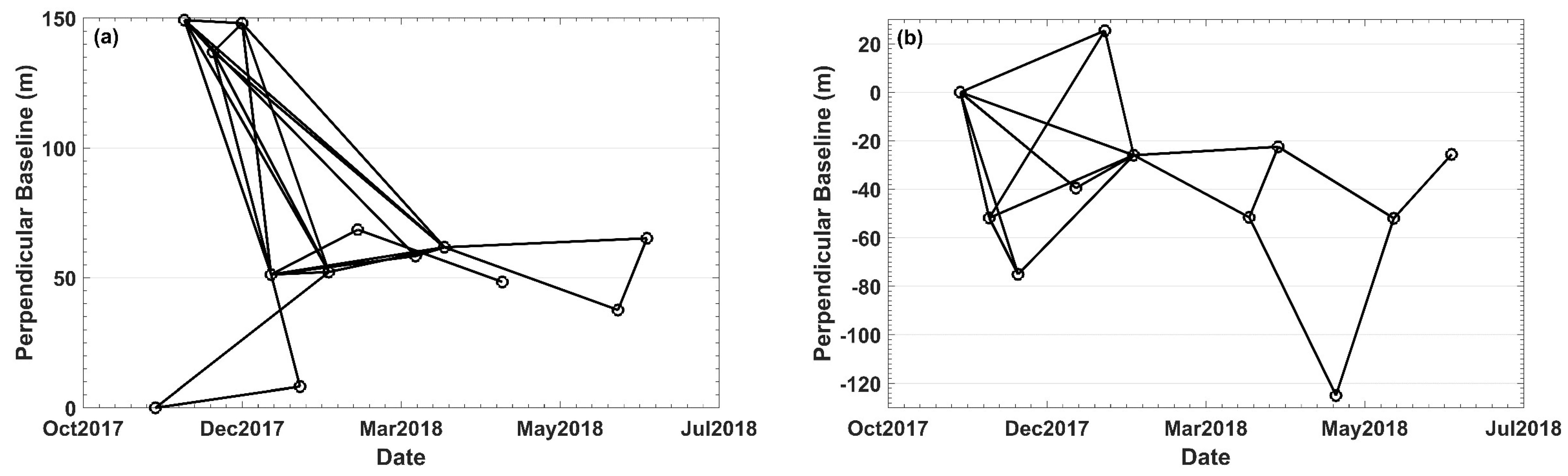
3.1. Data used in this Study

In this study, Sentinel-1A SAR images from ascending and descending tracks covering the study area were collected. European Space Agency (ESA) launched the Sentinel-1A satellite, and SAR images were acquired in the terrain observation with progressive scans (TOPS) mode. The image coverage is outlined as white rectangles in Figure 1. Three interferograms from the ascending Path72 (hereafter referred to as A72), descending Path6 (hereafter referred to as D6), and descending Path79 (hereafter referred to as D79) were used to obtain the co-seismic deformation field; the details are provided in Table 2. For the post-seismic deformation time series, we collected a total of 35 SAR images from A72 and D6, which spanned 23 November 2017–15 June 2018 and 19 November 2017–11 June 2018, respectively. To remove the topographic phase, shuttle radar topography mission (SRTM) digital elevation model (DEM) with 30 m resolution (https://earthexplorer.usgs.gov/) was used. Precise orbits (https://qc.sentinel1.eo.esa.int) were used for orbital corrections.

3.2. Data Processing

Interferometric processing was performed with the GAMMA software. The two-pass InSAR method was utilized to produce co-seismic deformation interferograms [13,21]. To improve the signal-to-noise ratio (SNR), interferograms were multi-looked by a factor of 8 in range and 2 in azimuth to result in a ground resolution of about 29 × 28 m. The interferograms were filtered twice with an adaptive filter function that was based on the weighted power spectrum algorithm [22] with windows of 128 × 128 pixels and then 32 × 32 pixels. Phase unwrapping was performed with the minimum cost flow (MCF) algorithm based on the Delaunay triangulation [23]. A nonlinear least-squares adjustment of the observed phase over presumably stable areas was used to refine the nonlinear residual orbit error [24]. To minimize the topography-dependent effect of the atmospheric signal, the following linear model of the topographic height was applied in order to estimate and correct the tropospheric delay phase [25]:
φ a t m o = b 0 + b 1 * h g t ( x , y )
where φ a t m o is the atmospheric delay phase, b 0 and b 1 are undetermined coefficients, and h g t ( x , y ) is the elevation. Before the delay phase is estimated, the deformation region needs to be masked.
In order to obtain the time series of the post-seismic deformation, we processed the images using the MSBAS technique that was proposed by Samsonov and D’Oreye [16]. This technique is derived from the original small baseline subset (SBAS) and it can compute 2D, east-west (EW), and vertical (UD) time-series deformations from ascending and descending tracks [16,26]. The 2D time-series deformation maps using multi-track InSAR datasets were obtained by inverting the following matrix:
( cos θ sin φ A cos φ A λ L ) ( V E V U ) = ( ^ 0 )
where matrix A consists of time intervals between consecutive SAR acquisitions; θ and φ are the azimuth angle and incidence angle, respectively; L is a zeroth-, first-, or second-order difference operator; λ is a regularization parameter; V U and V E represent the UD and EW components of the ground deformation velocities, respectively; and, ^ represents the observed interferometric displacement.
All of the interferograms were produced from SAR scenes with temporal and perpendicular baselines of less than 120 days and 80 m, respectively. The differential interferograms were filtered and unwrapped using the same method that is described above for co-seismic processing. As shown in Figure 2, a total of 45 highly coherent interferograms were selected, 27 from the ascending track, and 18 from the descending tracks. Subsequently, the selected ascending and descending interferograms were geocoded and then resampled to a common grid. Finally, we used the MSBAS technique to compute the 2D time-series deformation from the temporally and spatially overlapping ascending and descending D-InSAR data (Figure 2).

4. Results and Analysis

4.1. Co-seismic Deformation Field

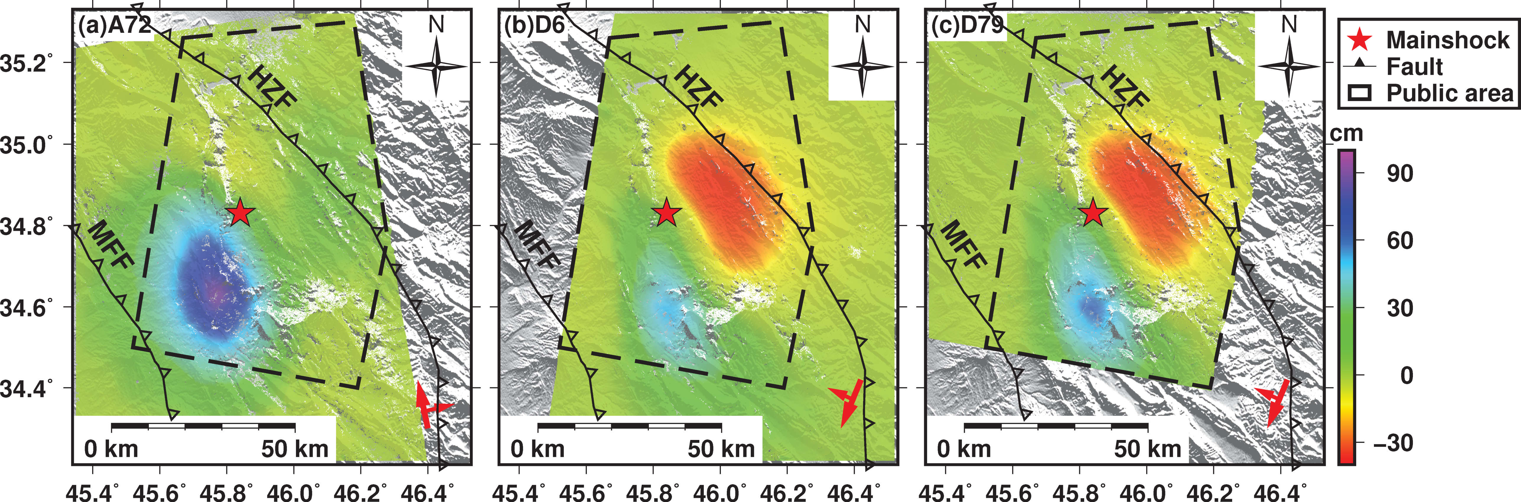
4.1.1. LOS Co-seismic Deformation Field

We processed the three selected interferograms (Table 2), and Figure 3 shows the LOS co-seismic deformation fields. A positive value indicates that the deformation in LOS was approaching the satellite; negative value indicates that deformation in LOS was moving away from the satellite. The three interferograms reveal clearly visible co-seismic deformation along the LOS. A72 showed a nearly circular LOS-direction uplift area with a diameter of about 70 km southwest of the epicenter, with a maximum deformation of about 90 cm. Northeast of the epicenter were fewer fringes with a deformation of 15 cm toward the satellite. D6 had co-seismic signals with a double elliptical pattern of deformation with maximum movements that were 50 and 38 cm toward and away from the satellite, respectively. D79 had a co-seismic deformation field that was consistent with that of D6, but the two patterns of deformation in the former were slightly larger, because the radar imaging geometries were different. The results from both the ascending and descending tracks reveal a clear co-seismic signal in the NNW direction, which is consistent with the direction of the strike angle that is given by the United States Geological Survey (USGS) and it is basically parallel with the MFF. Co-seismic deformation showed a continuous deformation pattern, which implies that the fault did not break the surface.

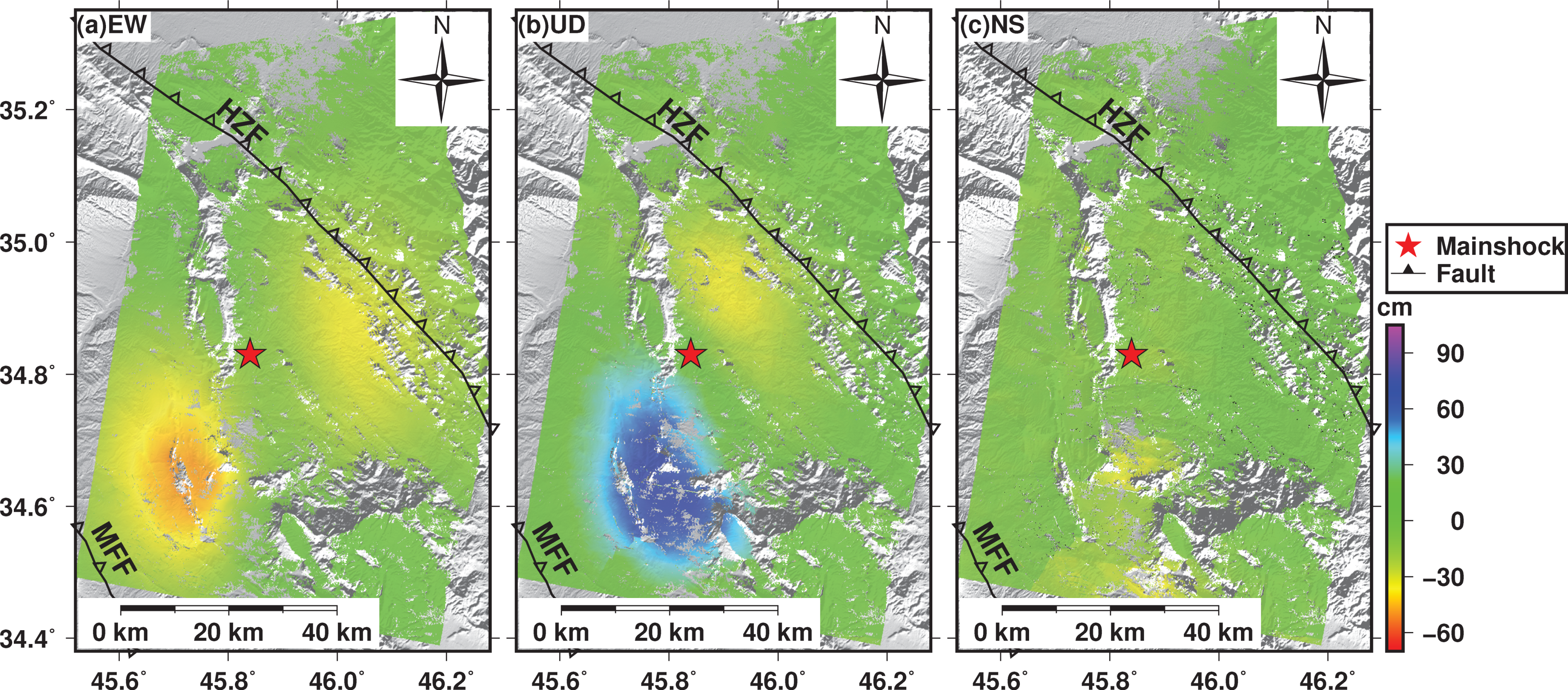
4.1.2. Three-dimensional Co-seismic Deformation Field

One limitation of InSAR is that it can only provide one-dimensional (1D) displacement measurements along the LOS; as such, ground deformation can be misjudged. For example, the Iran co-seismic deformation field along the LOS showed opposite signals northeast of the epicenter in the ascending and descending results. The 1D measurements are the projection of surface 3D deformation in the line of sight direction. According to the imaging geometry of SAR, the relationship between the 3D displacement and LOS displacement measurements can be described as [27]:
d l o s = d N sin θ sin φ d E sin θ cos φ + d U cos θ
where d l o s is the LOS deformation that was obtained by D-InSAR; d N , d E , and d U are the surface deformation components in the NS (north-south), EW, and UD directions, respectively; and, θ and φ are the incidence and azimuth angles, respectively (Table 2).
There are three unknown parameters in Equation (3). In theory, any three independent displacement measurements are sufficient in resolving the 3D displacement. We constructed the following equation:
F n × 3 × D 3 × 1 = d n × 1
where d n × 1 is the observation vector from the LOS observed displacement; D 3 × 1 is composed by the surface deformation components in the NS, EW, and UD directions, respectively; and, F n × 3 is the coefficient matrix formed by the corresponding projection vectors. The direct solution only requires the inverse of Equation (4). Owing to the side-looking geometry of the SAR sensor and its near-polar orbiting satellite platform, InSAR measurements are extremely insensitive to the north-south component; error amplification can be found in the combination of multiple InSAR measurements from different viewing geometries and the most exaggerated errors are noticeable in the north-south component [27].
Fortunately, by using an indirect solution, we acquired three image pairs with different imaging geometries. We reconstructed the 3D deformation fields of the Iran earthquake [28]. Previously, the error amplification phenomenon of the direct solution was shown to be significantly decreased with the indirect solution [14]. Therefore, we were able to derive a more reliable 3D co-seismic deformation field. Meanwhile, the features of the co-seismic surface deformation were better characterized. The 3D component matrix equations were then reconstructed under constraint conditions:
B n × 3 × D 3 × 1 + W n × 1 = 0
where W n × 1 is a constraint condition and B n × 3 is a conditional coefficient matrix. The indirect solution that was used in this study was the least-squares iterative solution to Equation (4) under the constraint of Equation (5). Based on the contribution of the 3D component to the LOS, the component with higher precision is selected as the constraint condition, and the values in the UD, EW, and NS directions are gradually iterated [28].
Figure 4 shows the derived 3D co-seismic deformation fields. Figure 4a shows that the two main displacement zones both had westward motions with maximum values of 52 and 45 cm southwest and northeast, respectively, of the epicenter. As shown in Figure 4b, ground uplift occurred southwest of the epicenter, with a maximum value of nearly 90 cm; ground subsidence occurred northeast of the epicenter with a maximum value of nearly 37 cm. Figure 4c shows an integrated southward motion. Overall, the 3D co-seismic deformation map shows a southwestward horizontal motion and continuous subsidence-to-uplift variation from the northeast to the southwest. The front edge of the subduction zone has a shallow dip angle. When the Iran earthquake occurred, the locked zone suddenly ruptured. The uplift zone was formed in front of the block near MFF, while the subsidence zone formed at the back end because of tension. Contrary to the Wenchuan event in 2008, the Iran earthquake caused both significant uplift and subsidence in the hanging wall.

4.2. Fault Geometry and Slip Distribution

The two-step inversion method was used to estimate the geometric parameters and slip distribution of the fault from three interferograms. First, we assumed that the earthquake was caused by a uniform slip and then performed an exhaustive search for the best-fit fault parameters. Subsequently, we divided the fault into sub-faults and used the linear inversion algorithm to estimate the slip that was distributed to each patch.

4.2.1. Uniform Slip Model

We used the open-source Geodetic Bayesian Inversion Software (GBIS; http://comet.nerc.ac.uk/gbis/) to apply nonlinear inversion to the fault geometry [29]. The inversion was carried out using a kinematic forward model as a rectangular dislocation source [30] with nine source model parameters: the length and width of the rectangular source, depth of the lower edge, dip angle with respect to the horizontal direction, strike angle of the horizontal edge with respect to the north direction, X and Y coordinates of the horizontal edge midpoint, strike-slip in the strike direction, and dip-slip in the dip direction. For the inversion, the optimal parameters and their uncertainties were estimated using the Markov chain Monte Carlo method (MCMC) that incorporated the Metropolis-Hastings algorithm [31,32]. Before the inversion, we subsampled the ascending and descending datasets with the quadtree method, and a total of 1887 data points were retained [33], which greatly reduced the computational complexity and enhanced the inversion accuracy.
Based on the fault geometry of the USGS results, we constrained the fault strike to vary from 180° to 360° and the dip angle to vary from 0° to 90° (https://earthexplorer.usgs.gov/). We set the iterations to 106, and the burn-in period of 3 × 10⁴ iterations was removed [29]. Finally, the best-fit solution was resolved from the uniform slip mode and all of the model parameters were well constrained according to their uncertainties. Table 3 presents the inversion results, which revealed that the co-seismic surface deformation was caused by a fault with a length of 38.08–38.87 km, width of 17.15–18.18 km, dip of 16.39°–18°, and strike of 355.39°–356.71°. For the Iran earthquake, the slip direction was consistent with that of a thrust fault with a right lateral component, with 2.75–2.96 m in the dip direction and −3.61 to −3.3 m in the strike direction. The fault was deeper than it was wide, which implies that it did not break to the surface. If the rigidity modulus of the region is assumed to be 30 GPa, then the computed optimal solution presented a seismic moment that was equal to 9.1 × 10¹⁹ N·m, which corresponds to a moment magnitude of MW 7.27. The results are in agreement with an oblique thrust slip on a shallow NE dipping fault, as suggested by the USGS. Figure 5 and Figure 6 compare the observed displacements, models, and residuals from the best-fitting parameters based on a uniform slip for both the ascending and descending data. The residuals of the uniform slip model were generally less than 5 cm (Figure 5c and Figure 6c), which confirms that the model fit the observed deformation reasonably well. However, relatively large residual signals were identified southwest of the epicenter, which are later discussed in Section 5.1.

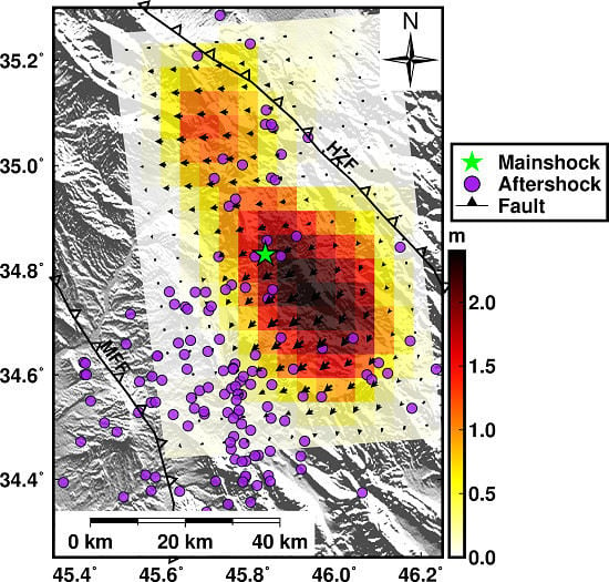
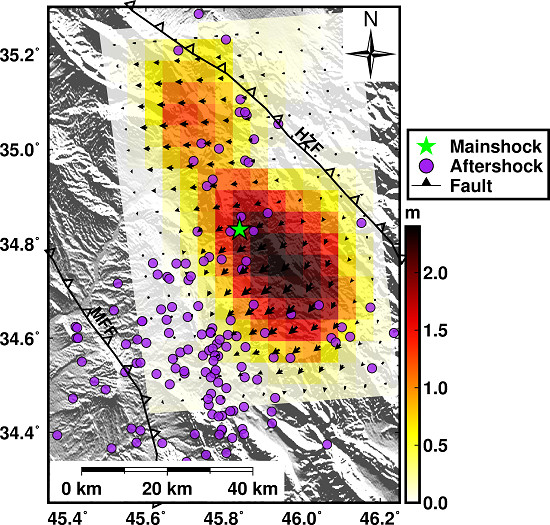
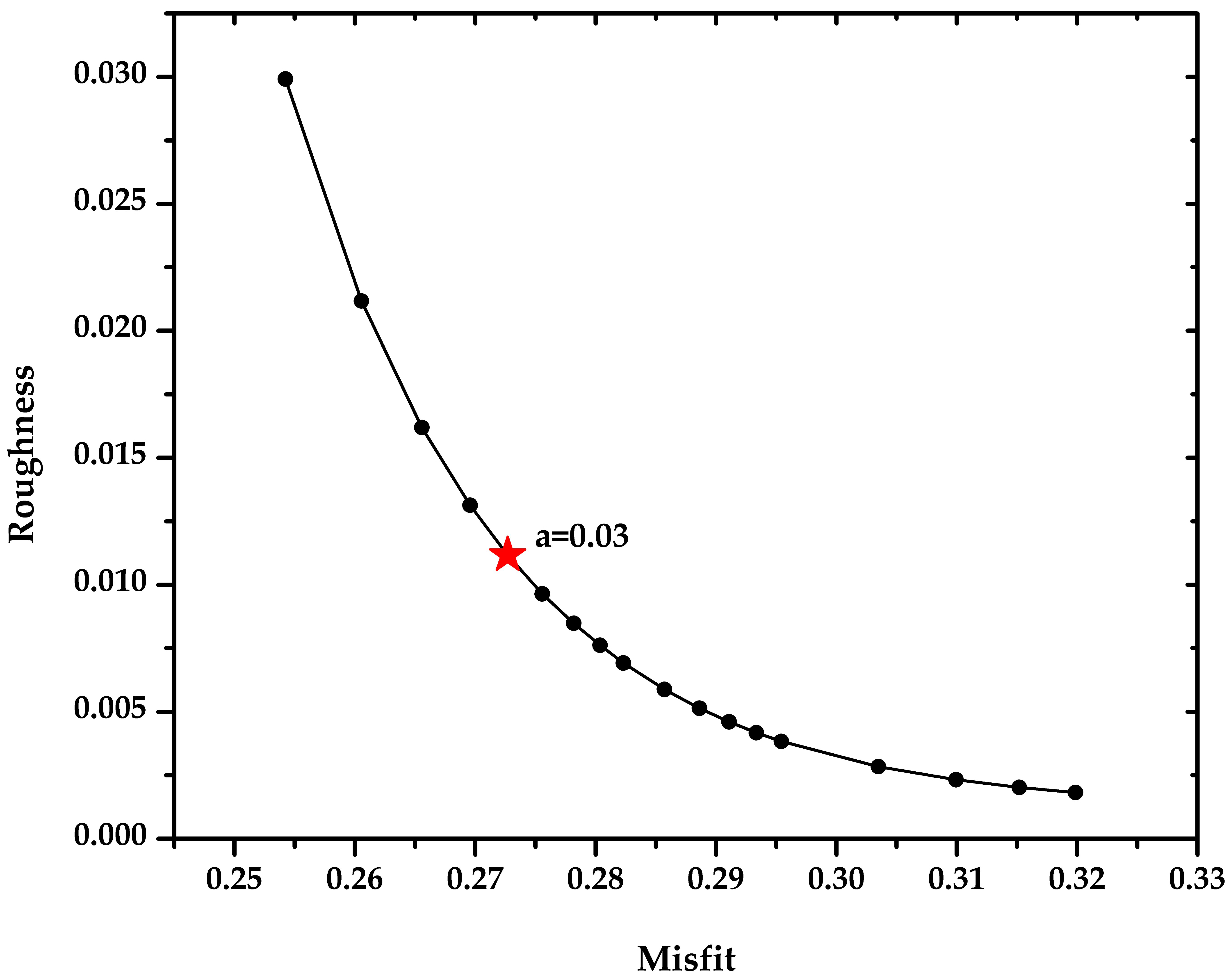
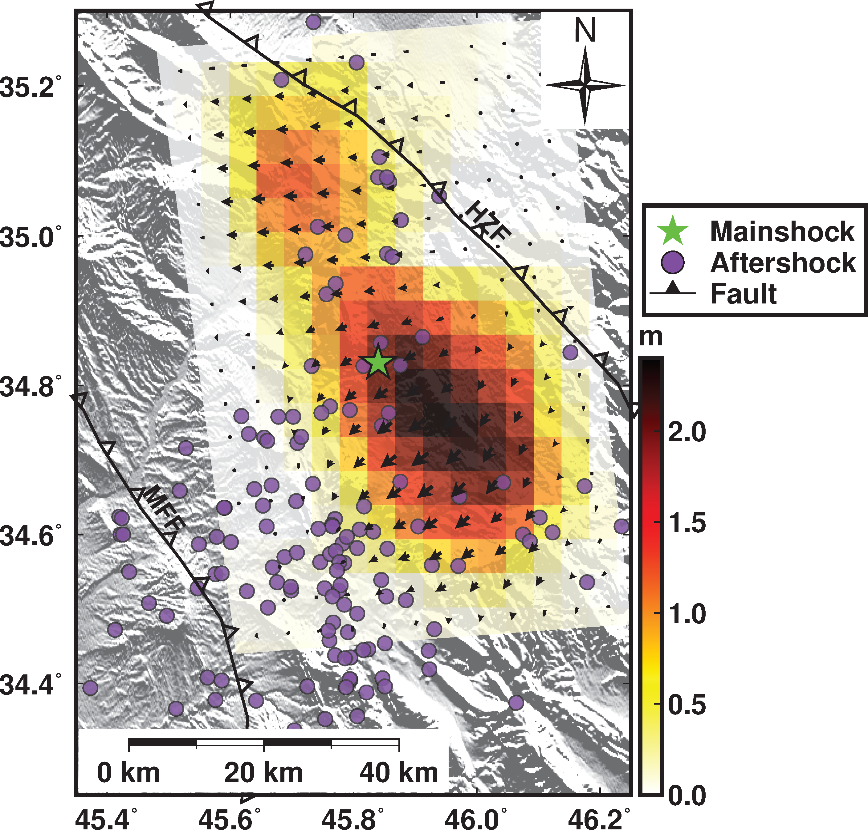
4.2.2. Distributed Slip Model

After the geometry of the seismological fault with uniform slip was determined based on Bayesian inversion, the motion parameters on the fault plane and the surface deformation were transformed into linear problems, and the co-seismic slip distribution was inversed by the steepest descent method (SDM) [34]. For the SDM inversion, parameters, such as the fault location, dip angle, and strike direction, were derived from the uniform slip model. In order to perform an exhaustive search in the potential space, we set a larger range and then expanded the fault along the strike direction and down the dip direction to 90 and 60 km, respectively, and it was divided into 18 along-strike and 12 down-dip patches, with areas of 5 × 5 km. To overcome the problem of the non-uniqueness and the instability of the inversion results, a smoothing constraint was applied to the slip distribution. Finally, we estimated the smoothing factor to be 0.03 by using an L-curve plot, as shown by the red star in Figure 7. We combined the ascending and descending observations and gave them the same weight. The thrust slip and right lateral components were allowed to freely vary on the fault plane. Subsequently, the slip on each patch was estimated with the SDM. The correlation coefficient between the observation and prediction was 98.6%. Figure 8 shows the projection of the distributed slip model on the ground. The heading of the arrow represents the slip vectors of each patch. The fault showed a thrust and slight right lateral slip motion. Along the strike, the rupture reached 80 km. The maximum slip was approximately 2.5 m, the macroscopic epicenter was at 45.97 °E, 34.76 °N, and the average rake angle and slip were 126.38° and 0.72 m, respectively. The geodetic moment that was based on the slip distribution was 1.16 × 10²⁰ N·m, which corresponds to MW 7.34. This is comparable to the seismological estimates, which ranged from MW 7.3 (USGS) to MW 7.4 (GCMT), as given in Table 1. In this study, the results demonstrate that the presence of two asperities in the shallow and deep subsurface; these are compatible with the results of Feng et al. and Ding et al. [9,11]. In addition, some results from the previous publications indicate there is one slip center in Iran earthquake [10,35]. However, it was worth noting that the slip model of the USGS was altered from single centralized, slipping to two asperities (last updated 17 October 2018).

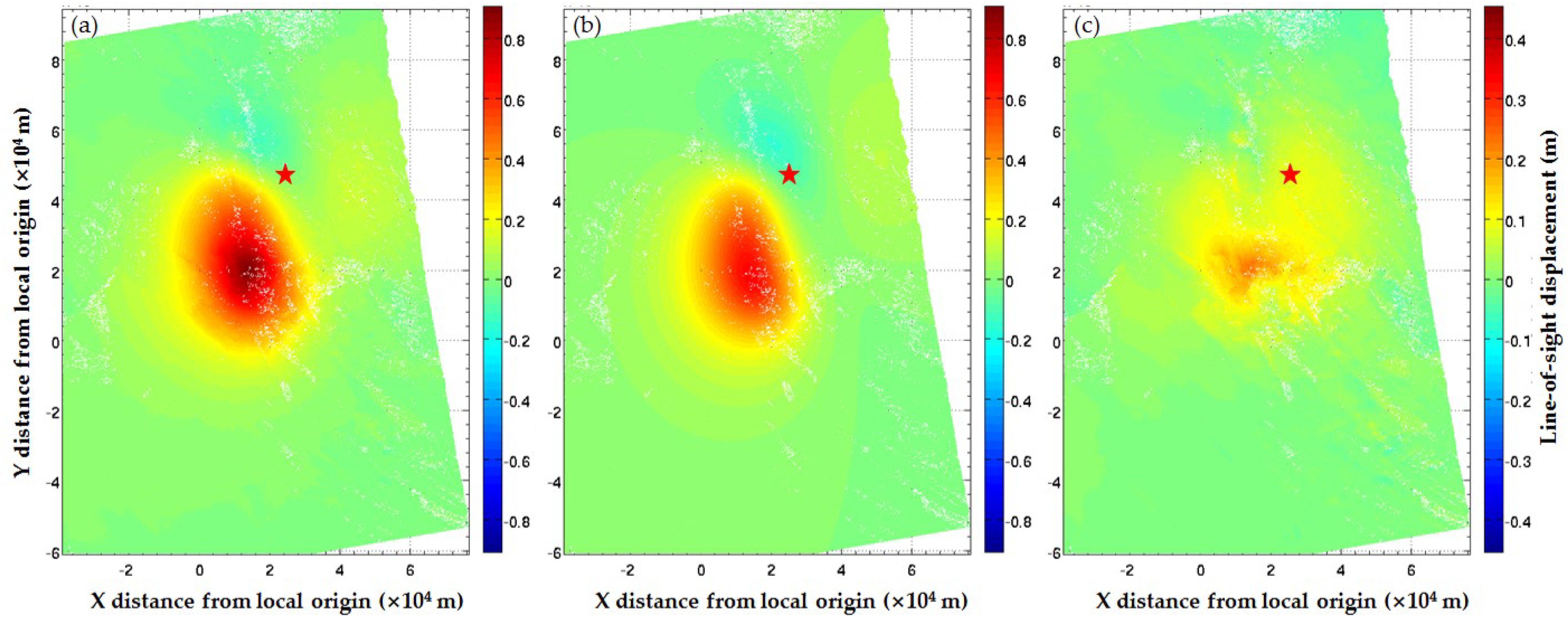
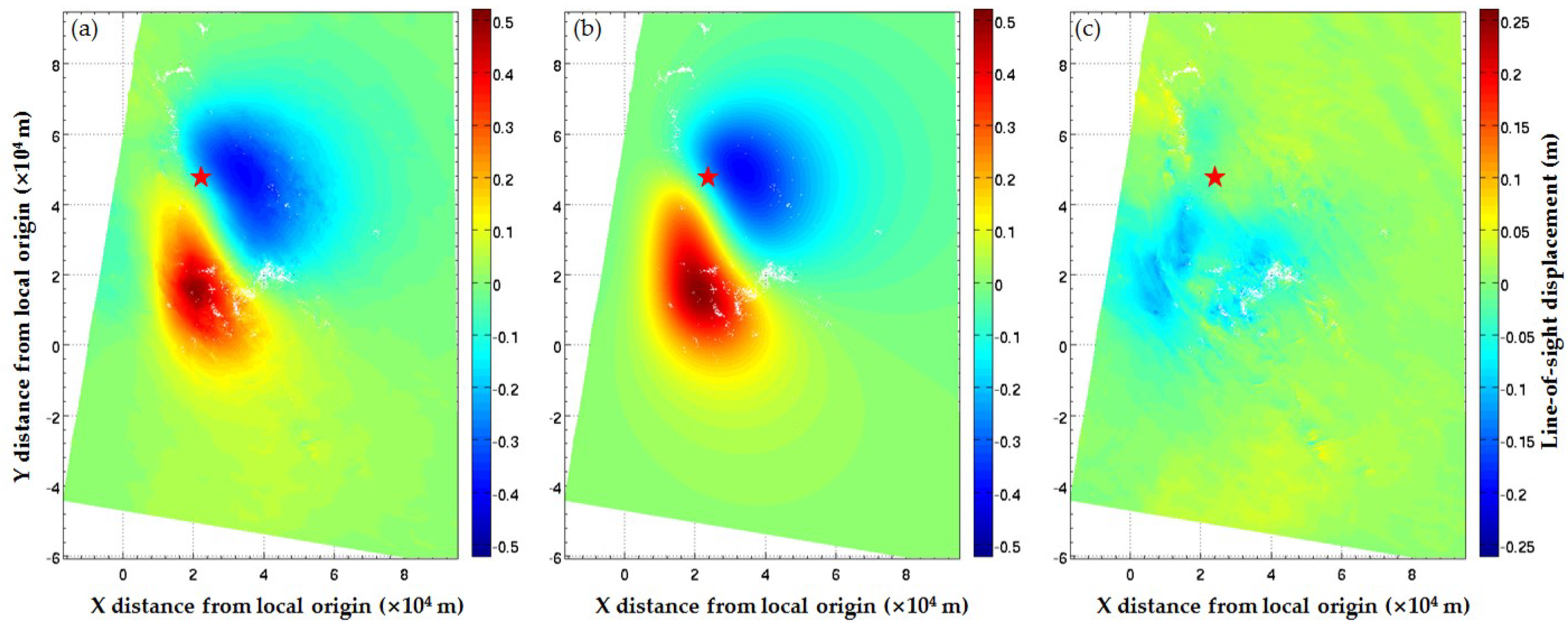
4.3. Two-dimensional Post-seismic Deformation Time Series

Post-seismic deformation following large earthquakes represents the redistribution of co-seismic stress changes in host rocks. Thus, continued study and geodetic observations are necessary in understanding the gestation of earthquakes and the detailed post-seismic deformation behaviors. In this study, we obtained the surface deformation within 220 days of the mainshock and investigated the spatial pattern of aftershocks, which is an important prerequisite for further understanding the nature of the causative fault. Previous studies have shown three possible post-seismic deformations after an earthquake: afterslip, poroelastic rebound, and viscoelastic relaxation [36,37]. All three factors likely play an important role: afterslip and poroelastic rebound in the near field and viscoelastic relaxation in the far field. Viscoelastic relaxation has a minor effect on near-field post-seismic displacement, especially in the short term [38]. Therefore, the effect of viscoelastic relaxation was not considered in this study.
According to the process that is described in Section 3.2, the UD and EW cumulative deformation maps were reconstructed with MSBAS. We selected eight dates of cumulative deformation in the UD and EW directions, as shown in Figure 9 and Figure 10, respectively. Cumulative post-seismic deformation increased with time. The time series of the 2D post-seismic deformation showed the same trend as the 3D co-seismic deformation in the directions of UD and EW (Figure 4a,b, Figure 9 and Figure 10). This similarity of co- and post-seismic interferograms suggests similar subsurface processes during both periods; specifically, it suggested that the dominant post-seismic process over the observation period was afterslip. As the same time, the references of [9] show that the poroelastic rebound had a minor effect for the Iran earthquake. Both co- and post-seismic deformation show two predominant patches. The post-seismic deformation steadily migrated to the southwest. Within 220 days of the mainshock, in the UD direction, the pattern of post-seismic deformation was distributed southwest of the epicenter, which is in contrast with the co-seismic deformation field (Figure 4a,b, Figure 9 and Figure 10). The maximum uplift displacement was 70 mm and the maximum subsidence was 35 mm. The southwestern patch accumulated larger afterslip when compared with the northeastern patch. In the EW direction, the two main displacement zones both had westward motions, with the maximum westward movement reaching approximately 45 mm. The mainshock changed the regional stress field, thus, the aftershocks occurred continuously. In order to reveal the relationship between afterslip and aftershocks, we collected the aftershock dataset (MW > 3.0) up to 220 days after the mainshock (from http://irsc.ut.ac.ir/bulletin.php). Figure 9h and Figure 10h plot the distribution of aftershocks; the aftershocks were concentrated in the MFF and they were consistent with afterslip deformation.
We extracted time-series deformation for three patches in order to analyze the characteristics of the time series for the post-seismic deformation (A, B, and C in Figure 9h and Figure 10h). Within 203 days of the mainshock, Patch A showed the cumulative deformation of −34 cm in the UD direction and −37 cm in the EW direction; Patch B showed cumulative deformation of 44 cm in the UD direction and −45 cm in the EW direction; and, Patch C was in the far-field area and the maximum deformation was 4 mm in the UD direction and −3 mm in the EW direction. Therefore, the uncertainty in the UD and EW directions can be assumed to be ±4 mm, which includes the atmospheric phase, temporal decorrelation, and so on. To understand the tendency of the post-seismic deformation, the data were fitted to the following logarithmic model [35,39]:
y = D + a × log 10 ( 1 + t )
where D is the initial displacement of the mainshock (mm), y is the cumulative deformation (mm), t is the time after the earthquake (day), and a is the amplitude. The co-seismic interferometric pairs covered the post-seismic period (Table 2) and unified the co-seismic deformation values up to seven days after the mainshock. The co-seismic deformation was then set as the initial value of D in Equation (6). Figure 11 shows the fitting results of patches A and B as solid lines. The post-seismic cumulative deformation time series of Patch A contained co-seismic deformation values of 271 and −135 mm in the UD and EW directions, respectively, and that of Patch B contained co-seismic deformation values of 179 and −279 mm in the UD and EW direction, respectively. The frequency of aftershocks (>MW 3.0), which occurred frequently within 20 days (a total of 214 occurrences), but then decreased gradually, is shown in the histogram in Figure 11.
Conjoint analysis of co- and post-seismic displacement (Figure 11; divided by the seven days after the mainshock) showed that post-seismic displacement had the same direction of motion as the co-seismic displacement. The rate of afterslip was highest immediately after the mainshock, and then decreased with time. The cumulative deformation gradually increased. Together, these observations supported the scenario that afterslip on the fault plane was the most likely mechanism that is responsible for the near-field post-seismic deformation, rather than poroelastic rebound. The post-seismic displacement tendency of Patch A in the UD direction was opposite to that of the co-seismic motion (Figure 11a), which is discussed in Section 5.2. The fitted curve in Figure 11 shows that fault activity gradually decayed during the 220 days following the mainshock, but it did not stop. Similarly, the histogram in Figure 11 shows some aftershocks 200 days after the mainshock. The temporal evolution of afterslip and aftershocks of the Iran earthquake are consistent. With the deceleration of afterslip, the number of aftershocks fell, indicating a correlation between afterslip and the number of aftershocks. Our results are consistent with a previous study, which reported that afterslip governs the temporal evolution of aftershocks [40].

5. Discussion

5.1. Co-seismic Deformation

Our analysis of co-seismic deformation from both ascending and descending data (Figure 3) shows that patterns in the southwest are the same, while those for the northeast are diametrically opposite. This indicates that co-seismic deformation contained vertical and horizontal motions that were in line with the characteristics of a thrust slip with right lateral slip. The uniform slip model fits the observed deformation well. Relatively large residual signals were identified southwest of the epicenter (Figure 5c and Figure 6c), because the uniform slip model could not identify deformation that is caused by aftershocks. Generally, large earthquakes are followed by aftershocks in response to co-seismic stress changes. In the larger slip area, the original accumulated stress was fully released during the mainshock, and fewer aftershocks occurred in this area (Figure 8). The accumulated stress was gradually released by the aftershocks in the smaller slip area, as shown in Figure 8. The slip distribution was well constrained in the MFF, and the distribution of aftershocks was also close to the MFF. We have demonstrated that the MFF was responsible for the earthquake. The co-seismic interferograms that were derived from SAR data show a continuous deformation pattern, and the slip distribution was relatively small near the ground surface. These results indicate that the earthquake was a blind rupture event.

5.2. Post-seismic Deformation

We used the MSBAS technique to compute a time series of post-seismic 2D deformation during the 220 days following the mainshock. The co- and post-seismic slip tendencies (Figure 11) indicate that afterslip was the most likely mechanism that is responsible for the post-seismic deformation. Our results show that 3D co-seismic deformation was distributed on two sides of the epicenter in the UD and EW directions (Figure 4), while post-seismic deformation was southwest of the epicenter (Figure 9 and Figure 10). The position of the post-seismic uplift maximum was located southwest of the peak co-seismic slip (Figure 4b and Figure 9). Together, these might indicate that stress was relieved towards the MFF after the mainshock, and that the subduction process pushed up the front of the block near MFF. At the same time, the back block gradually subsided because of tension, and the subsidence area also moved to the front of the Zagros Mountains. Figure 11a shows that the post-seismic slip tendency of Patch A changed during the co- and post-seismic periods. This is expected, because part of the uplift was counteracted by the subsidence induced by the afterslip. Furthermore, we noticed that two earthquakes with MW 6.0 and MW 6.3 occurred around the epicenter on 25 August and 25 November 2018, respectively (Figure 9h and Figure 10h). Whether these two earthquakes were triggered by the mainshock will be the focus of future work. All of the signs indicate that seismic activity is intense near the MFF, and so closer attention should be paid to this region.

6. Conclusions

Based on Sentinel-1A SAR images from the ascending and descending tracks, we used the InSAR technique to study the co- and post-seismic deformations of the MW 7.3 Iran earthquake on 12 November 2017. We came to the following conclusions:
  • We acquired co-seismic deformation fields from three radar imaging geometries. Subsequently, we derived the 3D co-seismic deformation fields. The results show that the displacement field had a significant uplift of up to 90 cm southwest of the epicenter, a moderate subsidence of up to 15 cm northeast of the epicenter, and a southwestward horizontal motion. The data suggest that the Iran earthquake occurred at a shallow dip angle subduction zone that is located on the Eurasian Plate and that the MFF was responsible for the mainshock.
  • Our estimations of the strike, dip, and rake retrieved with a uniform slip and distributed slip agree with the USGS solution that is based on body waveform data. The uniform model reveals that co-seismic surface deformation was caused by a fault with a length of 38.5 km, width of 17.7 km, and strike and dip angles of 356° and 17°, respectively. The slip distribution showed that the maximum slip was approximately 2.5 m. The average rake angle and slip were 126.38° and 0.72m, respectively. If the rigidity modulus of the region is assumed to be 30 GPa, then the seismic moment based on the slip distribution was 1.16 × 10²⁰ N·m, which is equivalent to Mw 7.34. This earthquake was a thrust fault event with a slight right lateral slip component.
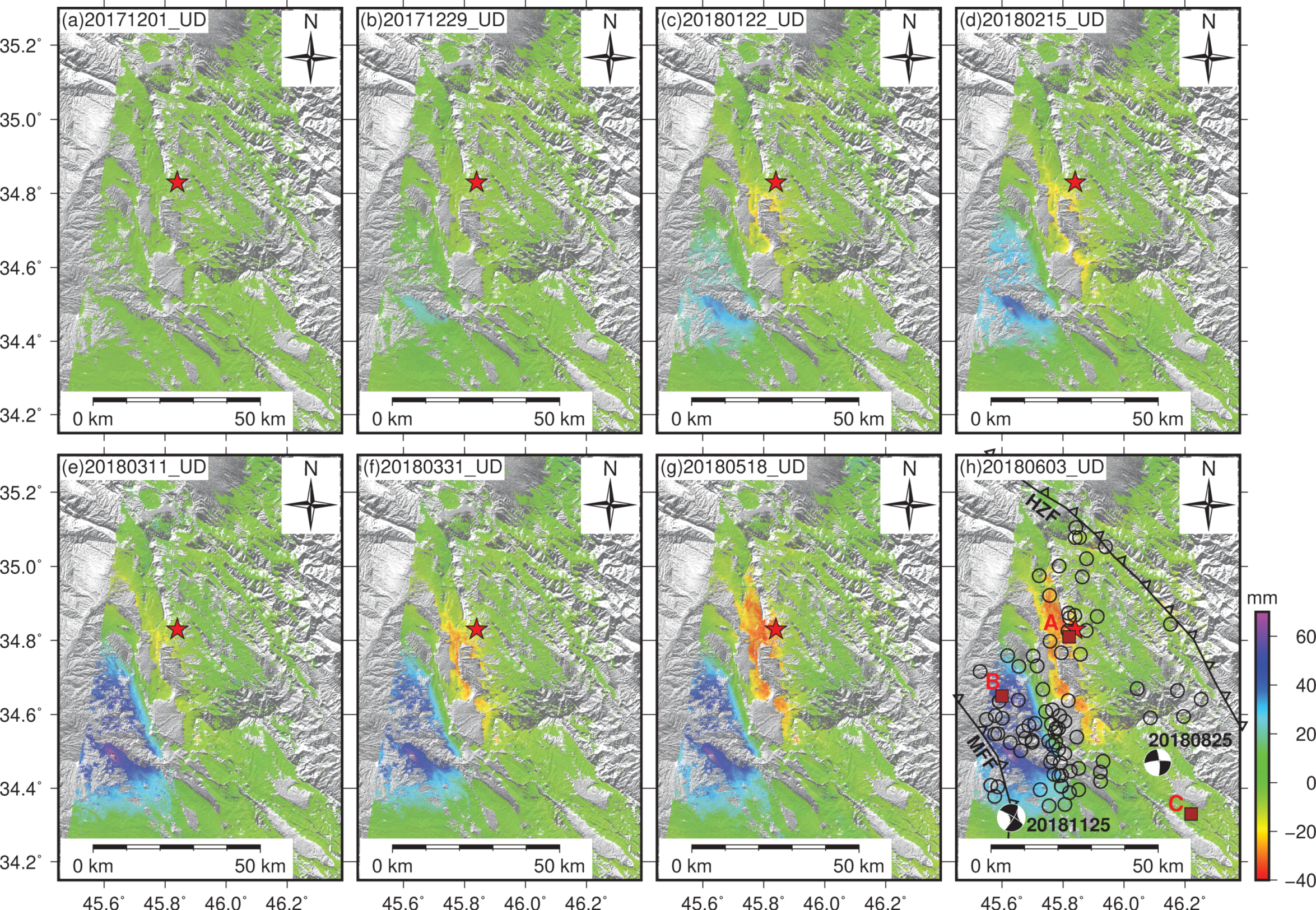
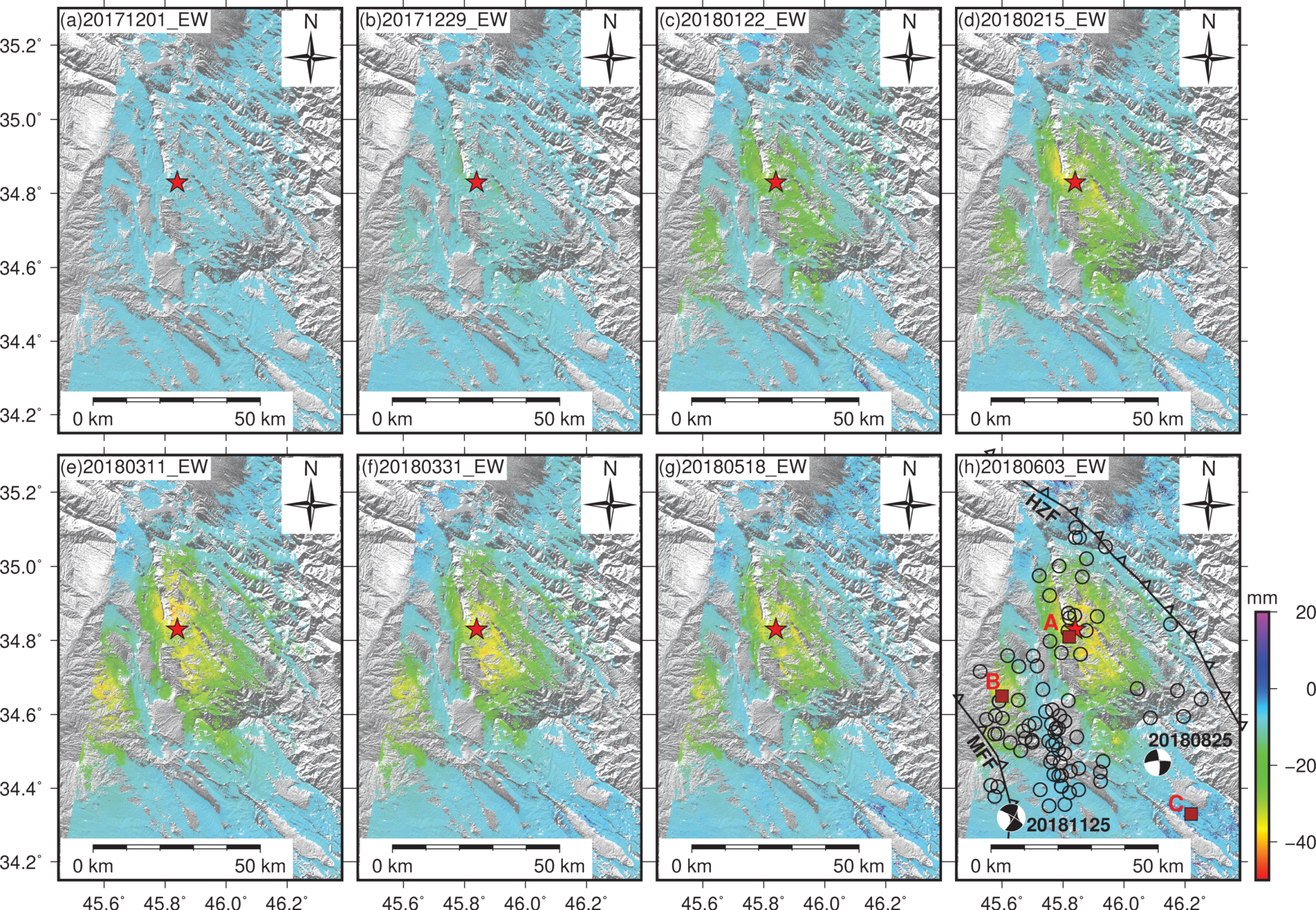
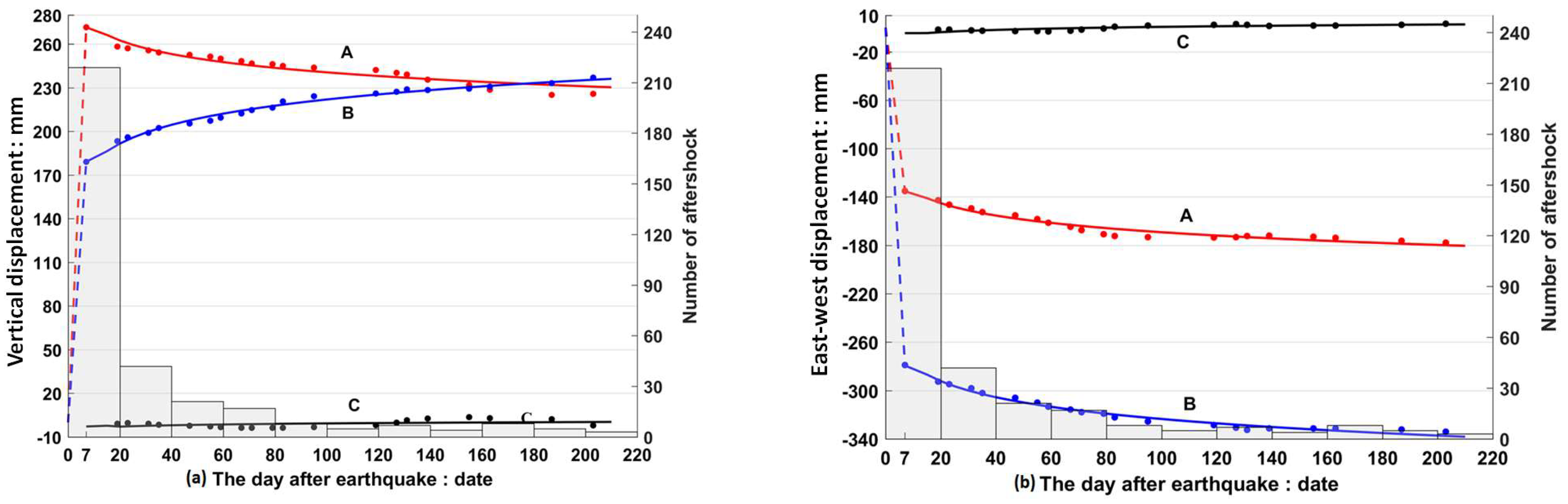
  • The MSBAS technique was used to obtain the time series of the 2D post-seismic deformation. The results show that the post-seismic surface in the UD and EW directions was consistent with that of 3D co-seismic deformation. Uplift occurred in the southwest (around patch B), while subsidence occurred in the northeast (around patch A). The maximum uplift and subsidence were 70 and 35 mm, respectively. In the east-west direction, there was westward motion with a maximum of approximately 45 mm. During the remainder of November, 214 aftershocks of Mw > 3.0 occurred; subsequently, there were a few more seismic events. The fault activity in this area gradually fell during the 220 days after the mainshock. Afterslip was a dominant part of the near-field post-seismic displacement, which also governed the temporal evolution of the aftershocks.
Our study helps in understanding the characteristics of regional fault activity and providing reliable scientific information for risk assessment pertaining to aftershocks. The Coulomb failure criterion has become a crucial quantitative index for the investigation and interpretation of mainshock-aftershock dynamics. However, this study did not address the Coulomb stress or aftershock inversion; these will be the focus of our future studies.

Author Contributions

C.Y., C.Z., conceived and designed the experiments; B.H. performed the experiments and drafted the manuscript; J.D., D.Z., and S.Z. contributed to the InSAR data analysis.

Funding

This research was funded jointly by the National Natural Science Foundation of China (grant numbers 41731066, 41628401, 41790445, 41604015, and 41604001), the National Key Research and Development Program of China (grant number 2018YFC1504805), and the Special Earthquake Research Project of the China Earthquake Administration (grant number 201508009).

Acknowledgments

We thank the editor, Zhenhong Li, Wanpeng Feng and three anonymous reviewers for their constructive suggestions. We acknowledge the European Space Agency (ESA) for freely making available the Sentinel-1A data. Maps were prepared using the Generic Mapping Tools (GMT) and MATLAB software.

Conflicts of Interest

The authors declare no conflict of interest.

References

  1. Zare, M.; Kamranzad, F.; Parcharidis, I. Preliminary Report of MW7.3 Sarpol-e Zahab, Iran Earthquake on November 12. 2017. Available online: http://www.emsc-csem.org/Files/news/Earthquakes_reports/Preliminary_report_M7.3_20171112_v3.pdf (accessed on 1 April 2018).
  2. Zebker, H.A.; Rosen, P.A.; Goldstein, R.M.; Gabriel, A.; Werner, C.L. On the derivation of coseismic displacement fields using differential radar interferometry: The Landers earthquake. J. Geophys. Res. Solid Earth 2002, 99, 19617–19634. [Google Scholar] [CrossRef]
  3. Hanssen, R.F. Radar Interferometry; Springer: Dordrecht, The Netherlands, 2001. [Google Scholar]
  4. Fialko, Y.; Sandwell, D.; Simons, M.; Rosen, P. Three-dimensional deformation caused by the Bam, Iran, earthquake and the origin of shallow slip deficit. Nature 2005, 435, 295–299. [Google Scholar] [CrossRef] [Green Version]
  5. Tobita, M.; Nishimura, T.; Kobayashi, T.; Hao, K.X.; Shindo, Y. Estimation of co-seismic deformation and a fault model of the 2010 Yushu earthquake using PALSAR interferometry data. Earth Planet. Sci. Lett. 2011, 307, 430–438. [Google Scholar] [CrossRef]
  6. Feng, G.; Ding, X.; Li, Z.; Mi, J.; Zhang, L.; Omura, M. Calibration of an InSAR-derived coseimic deformation map associated with the 2011 MW-9.0 Tohoku-Oki earthquake. IEEE Geosci. Remote Sens. Lett. 2012, 9, 302–306. [Google Scholar] [CrossRef]
  7. Kobayashi, T.; Morishita, Y.; Yarai, H.; Fujiwara, S. InSAR-Derived Crustal Deformation and Reverse Fault Motion of the 2017 Iran–Iraq Earthquake in the Northwest of the Zagros Orogenic Belt. Available online: http://www.gsi.go.jp/ENGLISH/Bulletin66.html (accessed on 24 May 2018).
  8. Wang, Z.; Zhang, R.; Wang, X.; Liu, G. Retrieving three-dimensional co-seismic deformation of the 2017 MW7.3 Iraq earthquake by multi-sensor SAR images. Remote Sens. 2018, 10, 857. [Google Scholar] [CrossRef]
  9. Feng, W.; Samsonov, S.; Almeida, R.; Yassaghi, A.; Li, J.; Qiu, Q.; Li, P.; Zheng, W. Geodetic constraints of the 2017 MW7.3 Sarpol Zahab, Iran earthquake and its implications on the structure and mechanics of the northwest Zagros thrust-fold belt. Geophys. Res. Lett. 2018, 45, 6853–6861. [Google Scholar] [CrossRef]
  10. Vajedian, S.; Motagh, M.; Mousavi, Z.; Motaghi, K.; Fielding, E.J.; Akbari, B.; Wetzel, H.-U.; Darabi, A. Coseismic deformation field of the MW 7.3 12 November 2017 Sarpol-e Zahab (Iran) earthquake: A decoupling horizon in the northern Zagros Mountains inferred from InSAR observations. Remote Sens. 2018, 10, 1589. [Google Scholar] [CrossRef]
  11. Ding, K.; He, P.; Wen, Y.; Chen, Y.; Wang, D.; Li, S.; Wang, Q. The 2017 M w 7.3 Ezgeleh, Iran earthquake determined from InSAR measurements and teleseismic waveforms. Geophys. J. Int. 2018, 215, 1728–1738. [Google Scholar] [CrossRef]
  12. Massonnet, D.; Rossi, M.; Carmona, C.; Adragna, F.; Peltzer, G.; Feigl, K.; Rabaute, T. The displacement field of the Landers earthquake mapped by radar interferometry. Nature 1993, 364, 138–142. [Google Scholar] [CrossRef]
  13. Massonnet, D.; Feigl, K.L. Radar interferometry and its application to changes in the Earth’s surface. Rev. Geophys. 1998, 36, 441–500. [Google Scholar] [CrossRef]
  14. Liu, Y.H.; Gong, W.Y.; Zhang, G.H. Study of the D-InSAR deformation field and seismotectonics of the Aketao MW6.6 earthquake on November 25, 2016 constrained by Sentinel-1A and ALOS2. Chin. J. Geophys. 2018, 61, 4037–4054. (In Chinese) [Google Scholar]
  15. Wang, R.; Parolai, S.; Ge, M.; Jin, M.; Walter, T.R.; Zschau, J. The 2011 MW 9.0 Tohoku earthquake: Comparison of GPS and strong-motion data. Bull. Seism. Soc. Am. 2013, 103, 1336–1347. [Google Scholar] [CrossRef]
  16. Samsonov, S.; D’Oreye, N. Multidimensional time-series analysis of ground deformation from multiple InSAR data sets applied to Virunga Volcanic Province. Geophys. J. Int. 2012, 191, 1095–1108. [Google Scholar]
  17. McQuarrie, N. Crustal scale geometry of the Zagros fold–thrust belt. Iran. J. Struct. Geol. 2004, 26, 519–535. [Google Scholar] [CrossRef]
  18. Regard, V.; Bellier, O.; Thomas, J.-C.; Abbassi, M.R.; Mercier, J.; Shabanian, E.; Feghhi, K.; Soleymani, S. Accommodation of Arabia-Eurasia convergence in the Zagros-Makran transfer zone, SE Iran: A transition between collision and subduction through a young deforming system. Tectonics 2004, 23, TC4007. [Google Scholar] [CrossRef]
  19. Vernant, P.; Nilforoushan, F.; Hatzfeld, D.; Abbassi, M.R.; Vigny, C.; Masson, F.; Nankali, H.; Martinod, J.; Ashtiani, A.; Bayer, R.; et al. Present-day crustal deformation and plate kinematics in the Middle East constrained by GPS measurements in Iran and northern Oman. Geophys. J. Int. 2010, 157, 381–398. [Google Scholar] [CrossRef]
  20. Yang, B.; Qin, S.; Xue, L.; Zhang, K. Identification of seismic type of 2017 Iraq MW7.3 earthquake and analysis of its postquake trend. Chin. J. Geophys. 2018, 61, 616–624. (In Chinese) [Google Scholar]
  21. Wegmüller, U.; Werner, C. Gamma SAR processor and interferometry software. In Proceedings of the Third ERS Symposium on Space at the Service of Our Environment, Florence, Italy, 14–21 March 1997; European Space Agency: Paris, France, 1997; p. 1687. [Google Scholar]
  22. Goldstein, R.M.; Werner, C.L. Radar interferogram filtering for geophysical applications. Geophys. Res. Lett. 1998, 25, 4035–4038. [Google Scholar] [CrossRef] [Green Version]
  23. Eineder, M.; Hubig, M.; Milcke, B. Unwrapping large interferograms using the minimum cost flow algorithm. In Proceedings of the IEEE International Geoscience & Remote Sensing Symposium, Seattle, WA, USA, 6–10 July 1998; IEEE: New York, NY, USA, 1998. [Google Scholar]
  24. Rosen, P.A.; Hensley, S.; Zebker, H.A.; Webb, F.H.; Fielding, E.J. Surface deformation and coherence measurements of Kilauea Volcano, Hawaii, from SIR-C radar interferometry. J. Geophys. Res. Planets 1996, 101, 23109–23125. [Google Scholar] [CrossRef]
  25. Yang, C.-S.; Zhang, Q.; Qu, F.-F.; Zhang, J. Obtaining an atmospheric delay correction for differential SAR interferograms based on regression analysis of the atmospheric delay phase. Shanghai Land Resour. 2012, 3, 412. [Google Scholar]
  26. Samsonov, S.V.; D’Oreye, N. Multidimensional small baseline subset (MSBAS) for two-dimensional deformation analysis: Case study Mexico City. Can. J. Remote Sens. 2017, 43, 318–329. [Google Scholar] [CrossRef]
  27. Wright, T.J. Toward mapping surface deformation in three dimensions using InSAR. Geophys. Res. Lett. 2004, 31, 169–178. [Google Scholar] [CrossRef]
  28. Wen, S.-Y.; Shan, X.-J.; Zhang, Y.-F.; Wang, J.-Q.; Zhang, G.-H.; Qu, C.-Y.; Xu, X.-B. Three-dimensional co-seismic deformation of the Da Qaidam, Qinghai earthquakes derived from D-InSAR data and their source features. Chin. J. Geophys. 2016, 3, 912–921. (In Chinese) [Google Scholar]
  29. Bagnardi, M.; Hooper, A. Inversion of surface deformation data for rapid estimates of source parameters and uncertainties: A Bayesian approach. Geochem. Geophys. Geosyst. 2018, 19, 2194–2211. [Google Scholar] [CrossRef]
  30. Okada, Y. Internal deformation due to shear and tensile faults in a half-space. Bull. Seismol. Soc. Am. 1985, 75, 1018–1040. [Google Scholar]
  31. Hastings, W.K. Monte Carlo sampling methods using Markov chains and their applications. Biometrika 1970, 57, 97–109. [Google Scholar] [CrossRef]
  32. Mosegaard, K.; Tarantola, A. Monte Carlo sampling of solutions to inverse problems. J. Geophys. Res. Solid Earth 1995, 100, 12431–12447. [Google Scholar] [CrossRef] [Green Version]
  33. Jonsson, S. Fault slip distribution of the 1999 MW 7.1 Hector Mine, California, Earthquake, estimated from satellite radar and GPS measurements. Bull. Seismol. Soc. Am. 2002, 92, 1377–1389. [Google Scholar] [CrossRef]
  34. Wang, R.; Diao, F.; Hoechner, A. SDM—A geodetic inversion code incorporating with layered crust structure and curved fault geometry. In Proceedings of the EGU General Assembly, Vienna, Austria, 7–12 April 2013; European Geosciences Union: Munich, Germany EGU-2411. , 2013. [Google Scholar]
  35. Barnhard, W.D.; Brengman, C.M.J.; Li, S.; Peterson, K.E. Ramp-flat basement structures of the Zagros Mountains inferred from co-seismic slip and afterslip of the 2017 Mw 7.3 Darbandikhan, Iran/Iraq earthquake. Earth Planet. Sci. Lett. 2018, 496, 96–107. [Google Scholar] [CrossRef]
  36. Marone, C.J.; Scholtz, C.H.; Bilham, R. On the mechanics of earthquake afterslip. J. Geophys. Res. Solid Earth 1991, 96, 8441–8452. [Google Scholar] [CrossRef]
  37. Peltzer, G.; Rosen, P.; Rogez, F.; Hudnut, K. Poroelastic rebound along the Landers 1992 earthquake surface rupture. J. Geophys. Res. Solid Earth 1998, 103, 30131–30145. [Google Scholar] [CrossRef] [Green Version]
  38. Bie, L.; Ryder, I.; Nippress, S.E.J.; Burgmann, R. Coseismic and post-seismic activity associated with the 2008 M w 6.3 Damxung earthquake, Tibet, constrained by InSAR. Geophys. J. Int. 2013, 196, 788–803. [Google Scholar] [CrossRef]
  39. Yang, C.; Lu, Z.; Zhang, Q.; Zhao, C.; Peng, J.; Ji, L. Deformation at Longyao ground fissure and its surroundings, north China plain, revealed by ALOS PALSAR PS-InSAR. Int. J. Appl. Earth Obs. Geoinf. 2018, 67, 1–9. [Google Scholar] [CrossRef]
  40. Perfettini, H. Postseismic relaxation driven by brittle creep: A possible mechanism to reconcile geodetic measurements and the decay rate of aftershocks, application to the Chi-Chi earthquake, Taiwan. J. Geophys. Res. 2004, 109, B02304. [Google Scholar] [CrossRef]
Figure 1. (a) Shaded relief map of the study area. The red star represents the location of the mainshock (from www.globalcmt.org; named by date of occurrence in the format YYYYMMDD). Red triangles indicate aftershocks (MW > 5.0). Yellow circles indicate aftershocks (MW > 3.0) up to 220 days after the mainshock (from http://irsc.ut.ac.ir/bulletin.php). The white rectangles mark the coverage of the synthetic aperture radar (SAR) images. The red line denotes the boundary between the Arabian plate and Eurasian plate. The black lines are faults (MZF: Main Zagros Fault, HZF: High Zagros Fault, MFF: Zagros Mountain Front Fault). (b) Magnified image of the area denoted by the red box in (a), where the red line denotes the border between Iraq and Iran.
Remotesensing 11 00418 g001
Figure 2. Networks of post-seismic interference pairs from the (a) ascending and (b) descending tracks. For the multidimensional small baseline subset (MSBAS) analysis, 27 ascending and 18 descending track datasets were used, and the perpendicular baselines of all InSAR pairs were less than 80 m.
Remotesensing 11 00418 g002
Figure 3. Co-seismic interferograms from the ascending and descending tracks. (a) A72, (b) D6, and (c) D79. Black lines are faults. The dotted polygon indicates the common area of the ascending and descending tracks. Red stars represent the epicenter.
Remotesensing 11 00418 g003
Figure 4. Interferograms of three-dimensional (3D) co-seismic deformation. (a) east-west (EW) direction, positive and negative values represent eastward and westward movements, respectively. (b) Up-Down (UD) direction, positive and negative values represent uplift and subsidence movements, respectively. (c) North-south (NS) direction, positive and negative values represent northward and southward movements, respectively. Black lines are faults; red stars represent the epicenter.
Remotesensing 11 00418 g004
Figure 5. Uniform slip results of the ascending track: (a) observed, (b) synthetic, and (c) residual interferograms. Red stars represent the epicenter.
Remotesensing 11 00418 g005
Figure 6. Uniform slip result of the descending track: (a) observed, (b) synthetic, and (c) residual interferograms. Red stars represent the epicenter.
Remotesensing 11 00418 g006
Figure 7. Curve representing the tradeoff between the model roughness and misfit. The red star indicates the location of the optimal smoothing parameter.
Remotesensing 11 00418 g007
Figure 8. Slip distribution for the modeled seismic source. The cyan star is the epicenter. The purple circles indicate aftershocks (MW > 3.0) during the 220 days after the mainshock (from http://irsc.ut.ac.ir/bulletin.php). Black lines denote faults, HZF: High Zagros fault, MFF: Zagros Mountain Front Fault.
Remotesensing 11 00418 g008
Figure 9. Time series of the cumulative up-down (UD) deformation from 19 November 2017 to 3 June 2018 (positive and negative values represent uplift and subsidence, respectively). The black circles indicate aftershocks (MW > 3.0) up to 220 days after the mainshock. The brown squares represent the selected feature patch. The two beach balls represent earthquakes > MW 5.0. Red stars represent the epicenter.
Remotesensing 11 00418 g009
Figure 10. Time series of the cumulative horizontal east–west deformation from 19 November 2017 to 3 June 2018 (positive and negative values represent eastward and westward movements, respectively). The black circles indicate aftershocks (MW > 3.0) up to 220 days after the mainshock. The brown squares represent the selected feature patch. The two beach balls represent earthquakes > MW 5.0. Red stars represent the epicenter.
Remotesensing 11 00418 g010
Figure 11. Time series of the cumulative deformation. (a) Up-Down (UD) and (b) EW deformation. Red indicates Patch A. blue indicates Patch B. and black indicates Patch C. The dotted line indicates co-seismic deformation. Points indicate the cumulative deformation time series of the post-seismic deformation. The solid line indicates the fit of the cumulative deformation time series to the post-seismic deformation. The left Y axis represents the deformation, the right Y axis represents the number of aftershocks, and the X axis represents the number of days after the mainshock.
Remotesensing 11 00418 g011
Table 1. Focal mechanism solutions for the Iran earthquake.
Length (km)Width (km)Depth (km)Dip (°)Strike (°)Rake (°)Mean Slip (m)Lon (°)Lat (°)Magnitude (MW)
USGS a805019.016351137345.9634.917.3
GCMT b--17.911351140-45.8434.837.4
Vajedian et al.391618.7173541414--7.29
Feng et al.100801514.5351136>145.8734.737.32
Ding et al.483215.816.3354.7137645.2834.697.3
a United States Geological Survey. b Global Centroid Moment Tensor Catalogue.
Table 2. Detailed parameters of selected co-seismic interference pairs.
OrbitPathMaster ImageSlave ImageB (m) Δ t (days)Incident Angle (°)Azimuth Angle (°)
Ascending7220171030201711237.42443.85−12.97
Descending6201710262017111929.12443.89−167.02
Descending79201711122017112446.91234.09−169.46
Note: Master and slave images are named according to the acquired date in the format YYYYMMDD.
Table 3. Inversion results for the Iran earthquake.
ParameterOptimalMeanMedian2.5%97.5% a
Fault length (km)38.5438.4838.4838.0838.87
Fault width (km)17.7417.6717.6817.1518.18
Fault depth (km)20.1620.2220.2119.8720.58
Fault dip (°)17.0617.1917.1816.3918.00
Fault strike (°)355.90356.03356.07355.39356.71
Fault X (km)27.1127.0327.0426.5927.46
Fault Y (km)50.0250.0150.0149.7550.24
Fault StrSlip b (m)−3.40−3.45−3.44−3.61−3.30
Fault DipSlip c (m)2.852.852.852.752.96
a We obtained maximum posteriori probability solutions of 2.5% and 97.5% from the posterior probability density functions of the fault parameters. b The negative component of the strike-slip indicated that the hanging wall direction of motion was opposite to the strike; this was identified as right lateral slip. c The positive component of the dip-slip indicated that the hanging wall showed relative uplift; this was identified as a thrust fault.

