Article

L-Band UAVSAR Tomographic Imaging in Dense Forests: Gabon Forests

1
National Research Institute of Science and Technology for Environment and Agriculture (IRSTEA), University of Montpellier, Land Environment Remote Sensing and Spatial Information (TETIS), 34090 Montpellier, France
2
National Center for Remote Sensing, National Council for Scientific Research (CNRS), Riad al Soloh, 1107 2260 Beirut, Lebanon
3
Doctoral School of Sciences and Technologies, Lebanese University (LU), 1003 Beirut, Lebanon
4
Laboratory of Informatics, Robotics, and Microelectronics of Montpellier (LIRMM), University of Montpellier, 34392 Montpellier CEDEX 5, France
5
National Aeronautics and Space Administration (NASA), Jet Propulsion Laboratory (JPL), California Institute of Technology, Pasadena, CA 91109, USA
*
Author to whom correspondence should be addressed.
Submission received: 29 January 2019 / Revised: 18 February 2019 / Accepted: 20 February 2019 / Published: 26 February 2019
(This article belongs to the Section Forest Remote Sensing)

Abstract

:
Developing and enhancing strategies to characterize actual forests structure is a timely challenge, particularly for tropical forests. P-band synthetic aperture radar (SAR) tomography (TomoSAR) has previously been demonstrated as a powerful tool for characterizing the 3-D vertical structure of tropical forests, and its capability and potential to retrieve tropical forest structure has been discussed and assessed. On the other hand, the abilities of L-band TomoSAR are still in the early stages of development. Here, we aim to provide a better understanding of L-band TomoSAR capabilities for retrieving the 3-D structure of tropical forests and estimating the top height in dense forests. We carried out tomographic analysis using L-band UAVSAR data from the AfriSAR campaign conducted over Gabon Lopé Park in February 2016. First, it was found that L-band TomoSAR was able to penetrate into and through the canopy down to the ground, and thus the canopy and ground layers were detected correctly. The resulting TomoSAR vertical profiles were validated with a digital terrain model and canopy height model extracted from small-footprint Lidar (SFL) data. Second, there was a strong correlation between the L-band Capon beam forming profile in HH and HV polarizations with Land Vegetation Ice Sensor (LVIS) Level 1B waveform Lidar over different kinds of forest in Gabon Lopé National Park. Finally, forest top height from the L-band data was estimated and validated with SFL data, resulting in a root mean square error of 3 m and coefficient of determination of 0.92. The results demonstrate that L-band TomoSAR is capable of characterizing 3-D structure of tropical forests.

1. Introduction

Tropical forests have major impacts on Earth’s ecosystem in terms of carbon storage, regulating water, and weather. Above-ground biomass (AGB) is the most important parameter related directly to the amount of carbon in the global ecosystem cycle [1]. Uncertainty in balancing the global carbon budget arises from a deficiency in AGB density estimation and carbon stocks in tropical forests. Indeed, developing new technologies is critical in surveying and monitoring tropical forests. NASA, ESA, AGEOS, and DLR have developed united efforts in the implementation of the AfriSAR campaign in the Gabon forests [2]. In this context, the objective of the AfriSAR campaign was to acquire airborne and field data for the development, calibration, and validation of algorithms for the estimation of the vertical structure of tropical forests and the biomass within them. The airborne data provided by the campaign consist of polarimetric synthetic aperture radar (SAR) interferometry (Pol-InSAR), tomographic SAR (TomoSAR) datasets, Lidar full waveforms, and small-footprint Lidar (SFL).
SAR and Lidar provide records sensitive to 3-D forest structure parameters at high spatial resolution [3,4,5]. Lidar sensors emit a laser beam which is reflected by forest structure elements within the laser path, and the returned waveform is recorded by the Lidar system [6]. Metrics extracted from Lidar waveforms are used to estimate forests’ vertical structure. Concerning SAR, the development of approaches for the estimation of forest structure has been enhanced by the introduction of Pol-InSAR [7] and TomoSAR [8]. SAR is a coherent airborne or space-borne side-looking radar system that utilizes the flight path of the moving platform and offers high-resolution remote sensing imagery data. SAR has been a significant tool for a wide variety of landscape applications in a broad sense (e.g., natural habitats, rural areas, forests, natural hazards, urbanization) [9]. SAR data collected over 2-D synthetic aperture can be processed using signal processing algorithms to focus the illuminated scatters in 3-D space. Polarimetric SAR is an advanced imaging radar system [10] that plays an important role in radar remote sensing. Full polarimetry radar provides five datasets from each polarization band, namely, HH, HV (H: horizontal, V: vertical), VH, VV, and total power (TP). With polarimetric SAR, we can obtain much more information than a single polarized SAR system. Now polarimetric SAR has many applications, including agriculture (e.g., crop classification, soil moisture extraction) [11,12,13,14], oceanography (e.g., surface currents and wind field retrieval) [15], forestry (e.g., forest monitoring, classification, and tree height estimation) [16,17], and military (e.g., ship detection, target recognition/classification) [18,19].
TomoSAR is a multibaseline (MB) SAR technique that provides vertical resolution capabilities [8,20]. This technique has been repeatedly demonstrated using airborne data [8]. The potential of TomoSAR arises from its ability to identify forests’ top height, which is an essential parameter for AGB estimation [21,22]. Forest height estimation has been demonstrated using Pol-InSAR model inversion over different forests (i.e., boreal, temperate, and tropical) at multiple frequencies varying from P- up to X-band using airborne and spaceborne platforms [23]. Additionally, 3-D forest reconstruction by TomoSAR techniques is now well-established and has been demonstrated in various experiments in different forest ecosystems [21,22,24]. The ability of P-band TomoSAR to characterize the 3-D vertical structure of tropical forests has been discussed and evaluated [21], while the capabilities of L-band TomoSAR are still in a rather early stage of development. Using airborne data acquired during the TropiSAR campaign, Minh et al. [24] demonstrated that the use of tomographic imaging at L-band in tropical forests appears limited. The TropiSAR campaign carried out in 2009 in French Guiana offered the first opportunity to test TomoSAR in tropical forest areas. However, these data were suboptimal for assessing multi-frequency TomoSAR performance for forest structure monitoring. To overcome this limitation, the AfriSAR campaign was successfully carried out in 2015 and 2016, and acquired optimal tomographic and polarimetric data over dense forests in Gabon.
The aim of this paper was to analyze the capability of L-band TomoSAR to retrieve tropical forests’ 3-D structure and accurately estimate the top height of dense forests. First, we validated the L-band vertical profile with a digital terrain model (DTM) and canopy height model (CHM) from an SFL data-set as a reference. Second, qualitative comparisons of the Capon beam forming profile of the L-band at HH and HV polarizations with Land Vegetation Ice Sensor (LVIS) Level 1B waveform Lidar data were carried out over different regions of interest in Gabon Lopé National Park. In addition, forest top height was retrieved from the TomoSAR L-band data. The results suggest that L-band TomoSAR holds promise for mapping forest structure in tropical forests.
This paper is organized as follows: Section 2 describes the materials and methods used in our tomographic analysis. The validation of the results is illustrated in Section 3. Section 4 is devoted to discussing and interpreting the tomography results. Section 5 concludes the paper and states the future works.

2. Materials and Methods
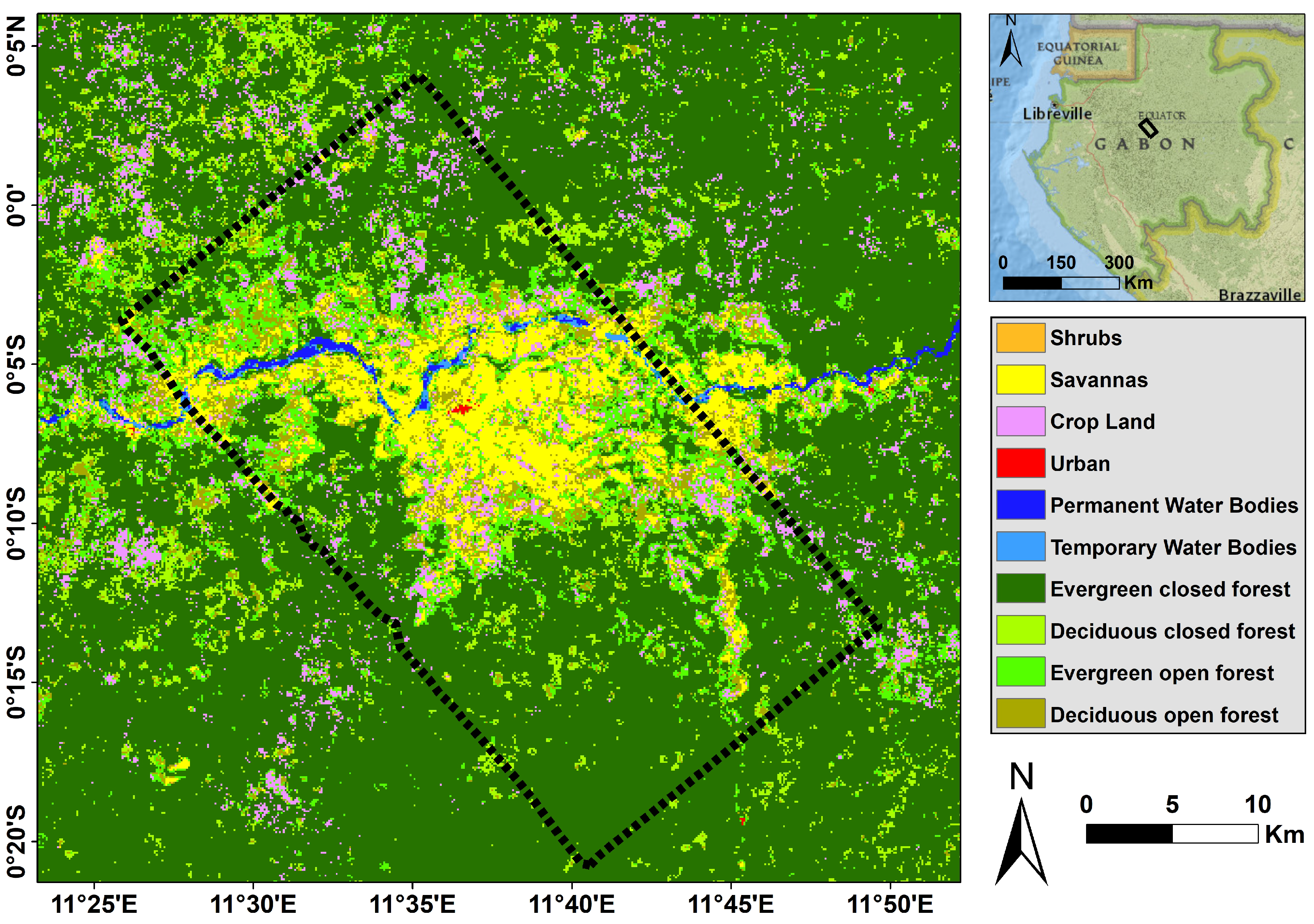
2.1. Study Area

The NASA-sponsored AfriSAR campaign was carried out over the tropical forests of Gabon in Africa. This campaign performed L-band UAVSAR acquisitions in February 2016. The campaign was conducted in collaboration with an ESA-sponsored campaign [25]. UAVSAR and Lidar systems flew over the same sites where ESA platforms acquired data. We will focus on the presentation of Lopé in which our tomographic study was conducted (Figure 1).
Lopé National Park is one of the largest national parks in central Gabon, covering an area of 4913 km 2 . Although the terrain is mostly rain forests, the scene in the northern part is composed of the last remnants of grass savanna created in Central Africa during the ice age 15,000 years ago. The park was the first protected area in Gabon. It is frequently tracked by the National Park Agency of Gabon, which makes it well-cited as a perfect scientific research site (Figure 1). This landscape consists of vast Savanna areas in the north, bounded by the Ogooué River and often burned to preserve the forests’ Savanna areas, in addition to an expanded region of compact tropical forests with patches of successive forests with complex structure, which are advanced through time with savanna recolonization [27]. Lopé is a convenient landscape to show the effective performance of UAVSAR for tomographic imaging due to the gradient of forest biomass from the forests’ savanna boundary (up to 100 Mg/ha) to compact undisturbed humid tropical forests (greater than 400 Mg/ha). Tree height and vertical structure can also vary gradually from savanna through forests, providing mono-dominant uniform trees of Okoumé (30–50 m tall) to regions with dense Marantaceae understory, and large gaps in mid-canopy, creating skewed vertical profiles. The topography of Lopé is also diverse, varying between large flat plains and steep sloping terrains. To achieve qualitative analysis between UAVSAR–TomoSAR vertical profile and Lidar waveforms, three regions of interest (ROIs) were selected. These regions include: two ROIs in the Okoumé-dominated forests (OKO1 and OKO2), and one ROI in colonizing forests (COL1) (Table 1).

2.2. Data-Sets

Different data-sets were acquired over Lopé Park during the AfriSAR campaign. The NASA AfriSAR campaign involved three data-sets: UAVSAR data, LVIS Lidar data, and SFL data.

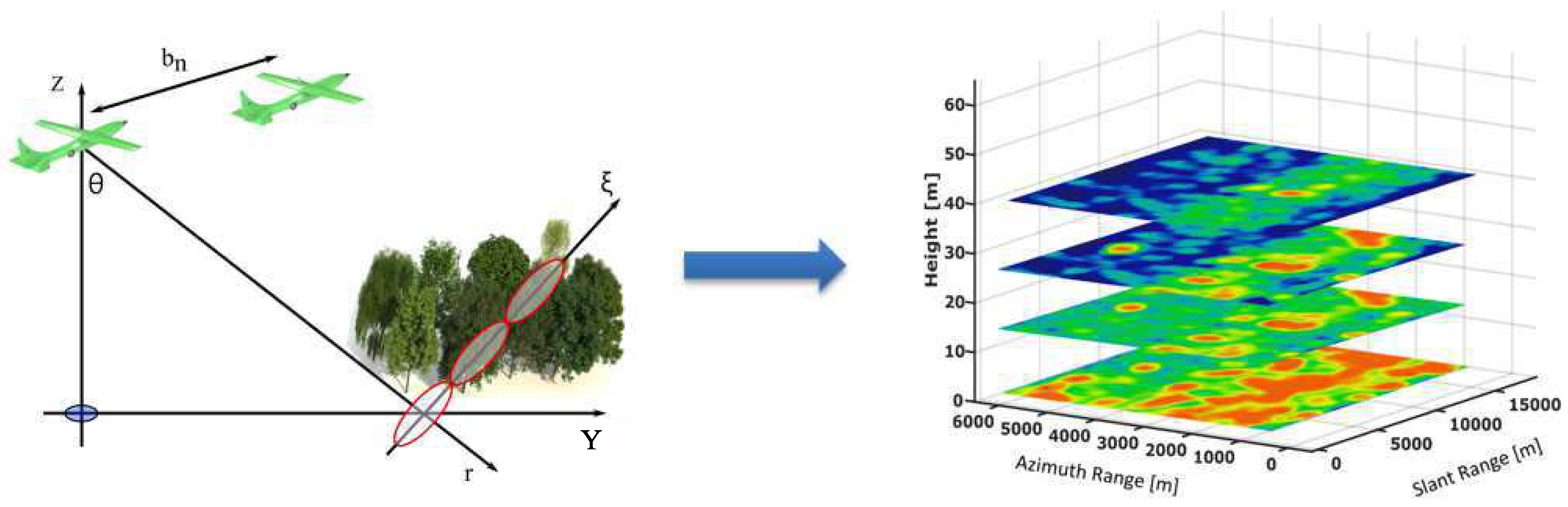
2.2.1. Radar Acquisitions Configuration

The AfriSAR campaign aims to provide support to forthcoming NISAR, GEDI, and BIOMASS missions. Using UAVSAR and the LVIS waveform Lidar instruments, NASA acquired 39.6 and 32.4 flight hours of data, respectively, over various sites in Gabon for the sake of calibration, verification, and new algorithm exposition of several ecosystem science products. The operating band of the UAVSAR radar instrument was 1217.5–1297.5 MHz (L-band; data can be downloaded from https://uavsar.jpl.nasa.gov/cgi-bin/data.pl), which exploits an electronically scanned array antenna to allow robust repeat-pass interferometric measurements [28]. The Gulfstream III jet, with an acceptable flight altitude of 12.5 km, allows the scanning of about a 22 km wide area, with incidence angles extending from 25 to 60 degrees. A typical UAVSAR polarimetric single-look complex (SLC) product has ground range and azimuth resolution of 2.5 m and 1.0 m, respectively [29]. In the following, we show the tomographic imaging over the northern part of Lopé National Park in Central Gabon using seven Pol-InSAR single-look-complex images collected by UAVSAR. The total area covered by the image was 22 km × 50 km, but a region of approximately 1 km × 5 km was considered for our study. The UAVSAR dataset acquired over Lopé is fully polarimetric, and was gathered by increasing the aircraft altitude by 20 m each flight track, leading to significantly low variation of vertical resolution from near range to far range. We present the acquisition parameters of UAVSAR configuration in Table 2, and the baseline configuration of the acquisitions is shown in Table 3.

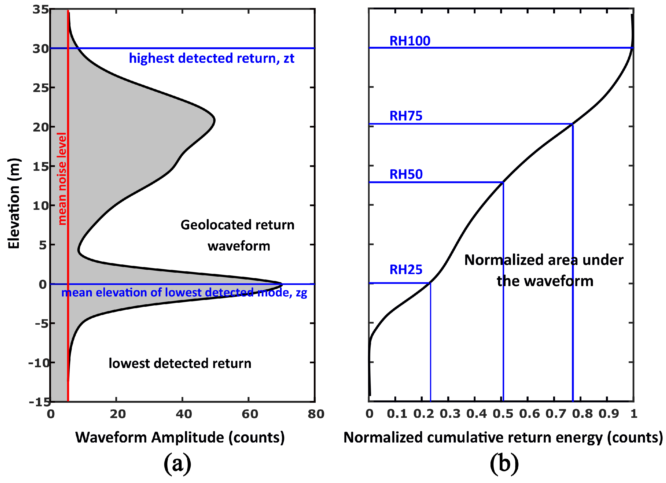
2.2.2. Lidar Data-Sets

Using different instruments, two Lidar data-sets were collected over the area of Lopé Park. The first data-set, which we will refer to as the SFL data-set, was acquired by Sassan Saatchi’s team (JPL) in July 2015 with a variable point density and footprint diameter of about 10 cm. The data-sets were pre-refined to eliminate any helicopter motion artefacts in order to present a more uniform point density of about 10 points per m 2 for vegetation characterization. i) DTM, ii) CHM, and other canopy metrics derived from CHM were derived from SFL data. Slope maps were estimated based on the DTM, and the heights of the Lidar point were normalized by removing the ground elevation. The DTM and CHM data were developed in a raster format at 1 m posting, characterizing the forest structure of an area of approximately 15 km 2 of old growth and successive forests, as well as savanna vegetation of the northern Lopé study site. The second Lidar data-set was acquired by NASA’s airborne Land Vegetation Ice Sensor (LVIS) during March 2016 as a part of the NASA–ESA collaboration of the BIOMASS, GEDI, and NISAR calibration and validation activities. LVIS is a large-footprint Lidar (LFL) with full-waveform capability with applications in measuring ground elevation and the vertical profile of vegetation structure in various ecosystems. There are two different datasets available for LVIS: Level 1B and Level 2 (data can be downloaded from https://lvis.gsfc.nasa.gov/Data/Data_Download.html). The level indicates the amount of processing undergone by the data before it was published. Level 1B data contain georeferenced Lidar returned waveforms. Level 2 data contain georeferencing information for different reflecting surfaces within the laser footprint, the locations of which were derived from the Level 1B waveform.

2.3. TomoSAR Background

TomoSAR implementation requires accurate handling regarding the relative phase difference between different passes. The rationale of TomoSAR is to employ multiple flight tracks that are nearly parallel to each other [21], as shown in the left panel of Figure 2. The ensemble of all flight lines allows the formation of a 2D synthetic aperture, resulting from the coherent multiple single-look complex (SLC) images of different passes, providing the possibility of focusing the signal in the entire 3D space. By exploiting tomography, SAR data can be converted into a new multi-layer SAR data stack where each layer represents scattering contributions associated with a certain height, as shown in the right panel of Figure 2 [21]. We will refer to ( r , x , ξ ) as the slant, azimuth, and cross ranges, respectively. We considered a data-set of SLC images acquired by N sensors in parallel track, and Y n ( r , x , ξ ) denotes the SLC value within pixel resolution cell ( r , x , ξ ) in the n-th image. The expression of topography-compensated (tc) SLC data can be approximated [30] as:
Y n ( r , x ) t c = P ( r , x , ξ ) e x p ( j 4 π λ r b n ξ ) d ξ ,
where P ( r , x , ξ ) denotes the projection of target reflectivity along the cross-range axis ξ ; and ξ represents the cross-range coordinate, orthogonal to the radar line-of-sight (LOS) that is defined by the slant range coordinate r. We can define k n , which is the wavenumber associated with the cross-range direction.
K n = 4 π λ R b n ,
where R is the distance from the sensor to the scatterer, λ is the carrier wavelength, and b n is the normal InSAR baseline with respect to the master track.

2.4. TomoSAR Phase Calibration

Prior to MB SAR algorithms, a fundamental issue should be taken into account, which is the phase calibration of the TomoSAR data, in order to compensate the phase residuals that influence the focusing of MB SAR data. These phase disturbances originate from atmospheric propagation delays or an error in allocating the platform position. To overcome this issue, we adopted UAVSAR data for phase calibration using an algebraic synthesis (AS) approach. This technique is an algebraic procedure to decompose ground and volume scattering based on multibaseline and multipolarimetric data [31]. This approach was already realized and validated at P-Band based on campaign data from BioSAR, BioSAR 2, and TropiSAR; see [22,32,33,34].
The TomoSAR data phase calibration using the AS approach was done by eliminating the ground-phase contributions from the tomographic SLC data. The exploitation of multipolarimetric and multibaseline (MPMB) data allows the identification of different scatterer mechanisms (SMs) [33]. The separation of the ground contribution and the vegetation from MPMB data was performed by presenting the data covariance matrix through the sum Kronecker product (SKP) [31].
The structural model of the data covariance matrix, where each SM is presented by the Kronecker product of two matrices, is addressed as follows:
W = E [ Y Y H ] = k = 1 N λ k C k R k C g R g + C ν R ν ,
where Y is the MPMB SLC data vector, H is the Hermitian conjugate, W denotes the data covariance matrix, k is the total number of SMs that contribute to the SAR signal, and C g , v and R g , v are the polarimetric signature and structure matrix corresponding to the ground and volume contributions, respectively.
The first step of phase calibration was to retrieve an initial guess for ground phases by applying Capon spectrum estimation using the HH channel, then the original data were corrected using this ground phase. Then, the ground phases were retrieved by the sum of Kronecker products (SKP) model. Assuming two main scattering mechanisms (i.e., ground and volume scatterings), we obtained the best LS approximation of the covariance matrix W by retaining the first two terms of the SKP Decomposition, and the matrices R g , R v , C g , and C v could be determined from the terms of the SKP decomposition via a linear transformation. Starting from initialization of ground phases, one can present the initial guess of ground phase at each track n by:
ϕ n i n i t i a l = 4 π λ r s i n θ n B n z g ,
where B n is the normal baseline relative to track n, r is the slant range for the whole scene, z g is the terrain topography, and θ n is the look angle associated to each track n:
z g = a r g m a x S c a p o n ( z ; H H ) .
Here, z denotes the vertical axis used to apply the spectrum estimation problem. Then, we can retrieve the ground phases at each track n, which can be expressed by:
ϕ n g r o u n d = 4 π λ r s i n θ B n z g + η n ,
where η n is the phase screen at track n. After the estimation of the ground covariance matrix, the phase linking algorithm is applied to estimate ground phases.
ϕ n g r o u n d = P L ( R g ) + ϕ n i n i t i a l ,
where PL denotes the phase linking algorithm [30]. Then, the calibration was carried out by removing ground phases from the original SLC data to obtain the calibrated SLC data.
Y n c a l = Y n . e x p ( j . ϕ n g r o u n d )
Finally, Capon beamforming power estimation was applied to get the tomographic profiles.

2.5. TomoSAR Inversion

SAR data were acquired over forests from slightly different altitude and incidence angles, providing useful information in the vertical direction [21]. The L-band UAVSAR airborne system provides a fully polarimetric mode in the NASA AfriSAR campaign. Tomographic techniques composed of power estimation methods were applied to the multibaseline SLC data to retrieve the backscattered power that characterizes the vertical profile of the forests [21,22]. In this paper, the Capon beam forming power estimator was applied to represent the vertical profile of vegetated areas.

Capon Beam Forming

Capon beam forming is a non-parametric power estimation method used in tomographic analysis that allows a continuous vertical profile to be obtained without any knowledge of the statistical properties of the data [35]. The Capon estimated vertical profile P c ( ξ ) is retrieved from the covariance matrix of the MB SLC data [36], and can be expressed as:
P c ( ξ ) = 1 a ( ξ ) t W 1 a ( ξ ) ,
where a( ξ ) is the steering vector containing the interferometric information for a scatter at cross range ξ for all the baselines relative to a master track, and W is the maximum likelihood estimation of the covariance matrix. Y denotes the multibaseline SLC data configuration. N is the number of tracks. Note that since the inverse of the estimated covariance matrix is used, the Capon estimator requires W to be well-conditioned in order to ensure that W 1 can be trusted.

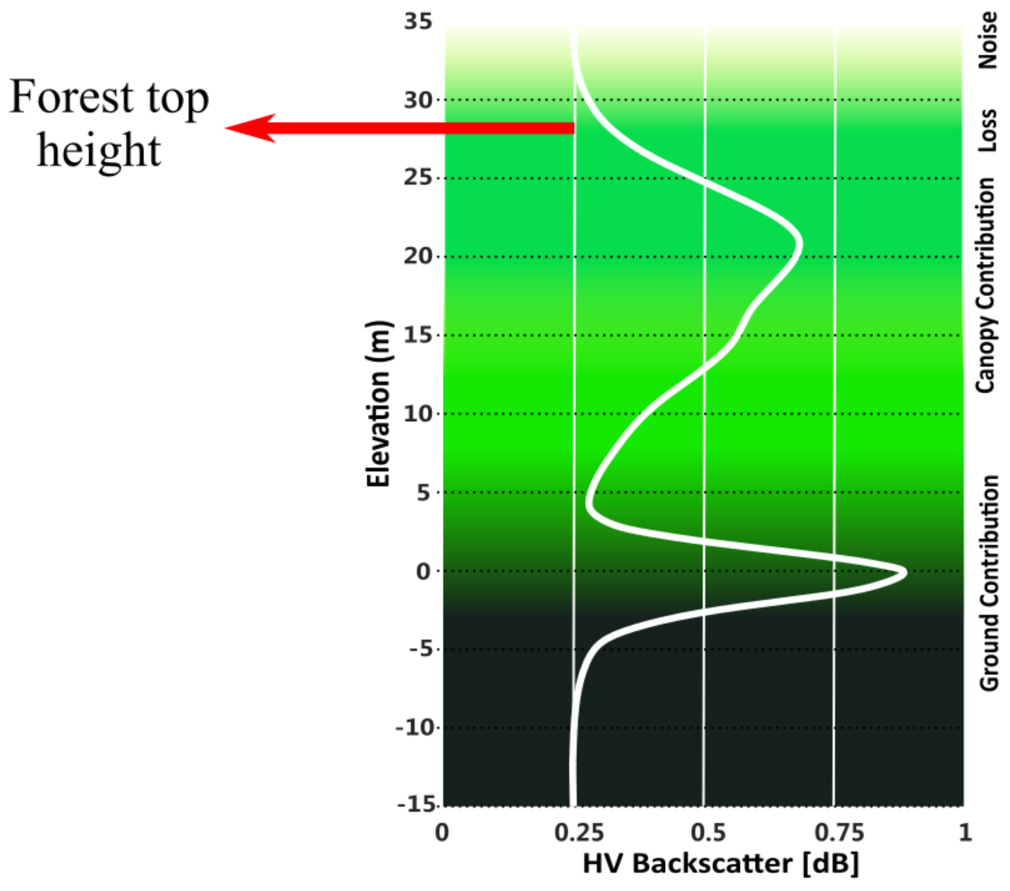
2.6. Estimate Forests’ Top Height
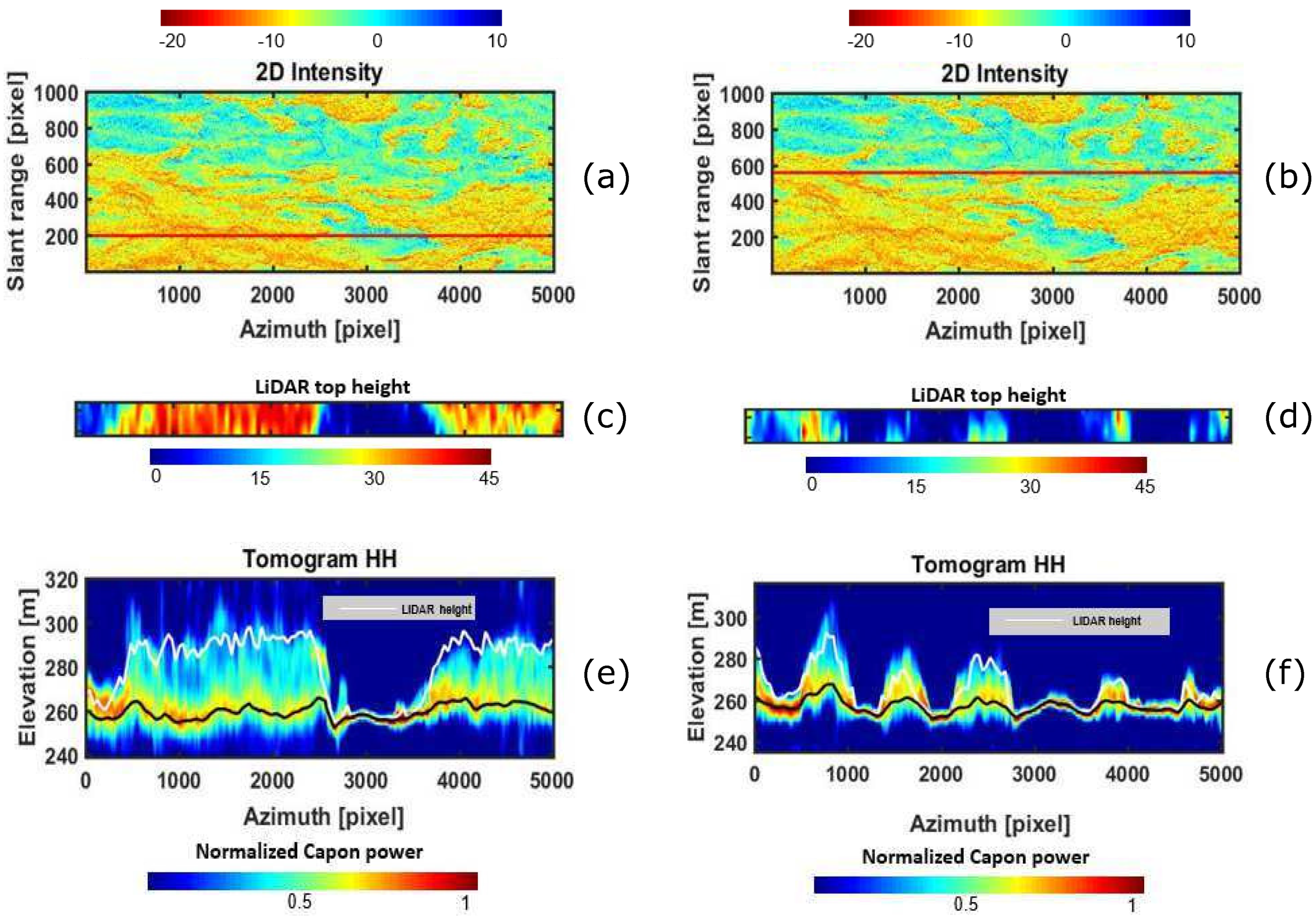
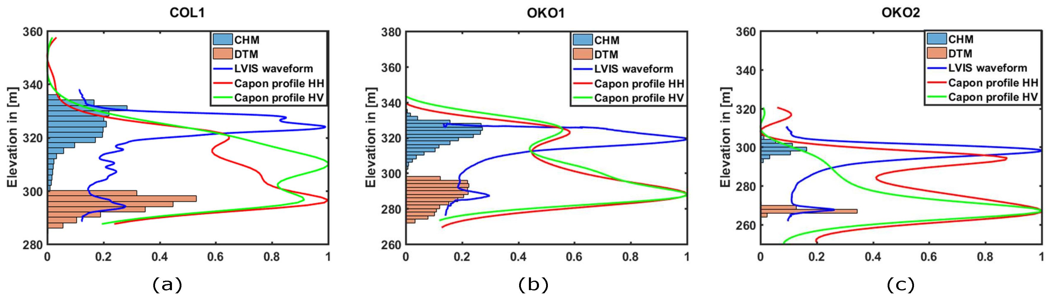
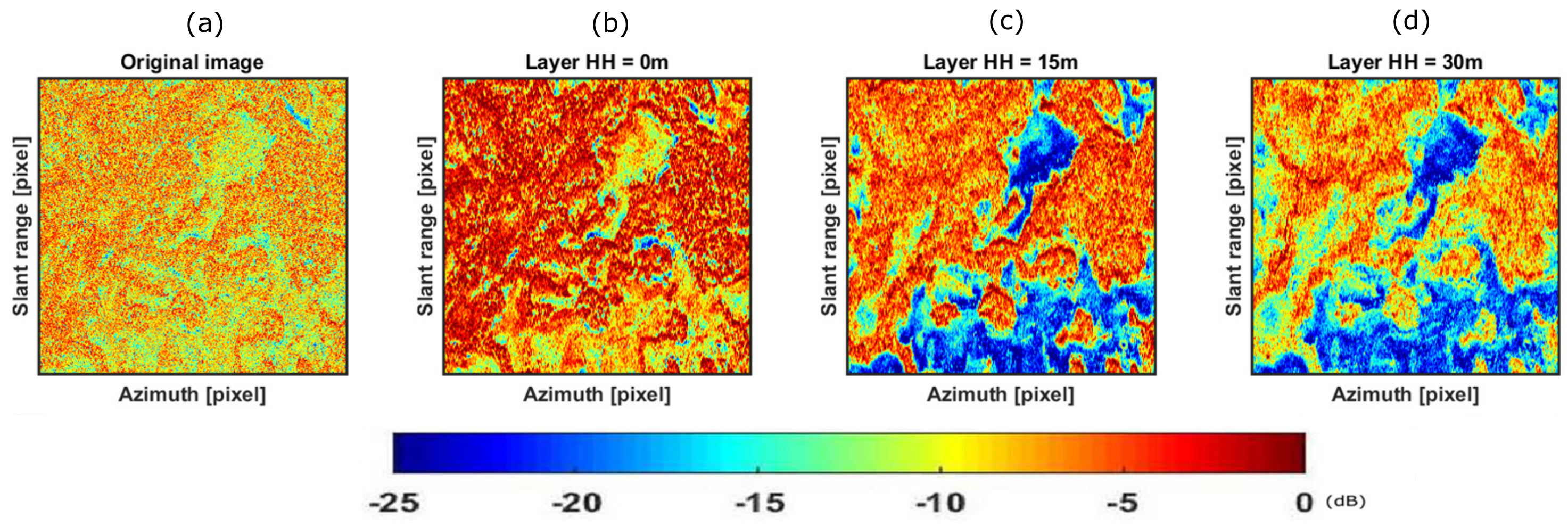
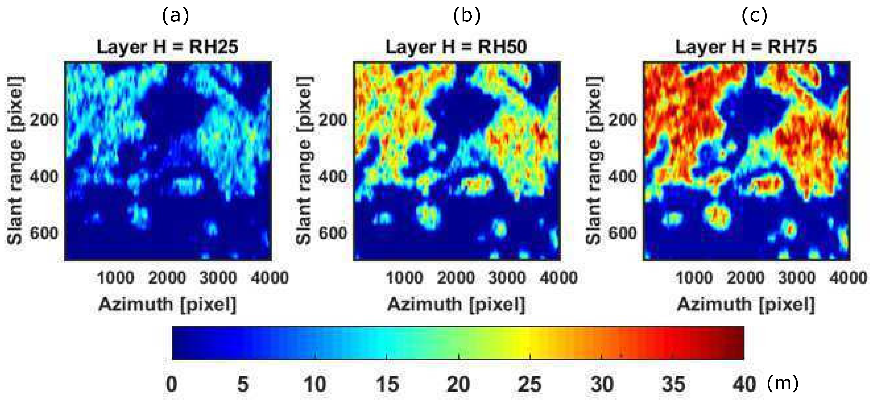
The canopy structure in tropical rain forests is more complex than any other forest type. The main challenge in such a field is the estimation of the forests’ top height because it is often difficult to clearly identify the top leaf or branch of a tree in the canopy. TomoSAR has been demonstrated as a powerful tool to estimate forests’ top height thanks to its accurate characterization of the vertical structure of tropical forests. Forests’ vertical structure can be observed by taking a tomographic profile, that is, a slice of the multi-layer data stack. Using the Capon beam forming power estimator, we can retrieve the 3-D backscatter distribution from the multi-layer SLC and show the vertical backscatter distribution function. Each vertical distribution is characterized by two effective contributions: one corresponding to the signal, where most of the backscatter is concentrated—the so-called Canopy contribution or phase center; and another contribution corresponding to the reflected signal from the ground. Figure 3 shows a schematic view of the vertical backscatter distribution in which it is assumed that the shape of the distribution can be divided into four zones. The first zone corresponds to the ground contribution, which is the signal reflected from the ground. The second one corresponds to the canopy layer contribution. The third one is the power loss zone, where the backscatter undergoes a loss along the vertical direction from the phase center (canopy contribution) location. Further away, the backscatter Capon profile is dominated by noise, unlikely to be associated with any physically relevant components. Forest top height can be retrieved by two different ways, either by identifying the power loss from the phase center location in the upper envelope of the profile or by identifying the power loss from the noise level (location of the highest return detected by the TomoSAR platform) to the forest’s top height.
H ( r , x ) = a r g m i n ( P ( H n , r , x ) P ( H c , r , x ) K ) ,
where P ( H n , r , x ) is the backscatter at the phase noise level, Hn is the elevation of the noise level, K is the power loss value, and Hc is the height value ranging from Hn down to the canopy peak elevation in the upper envelope of the profile. Since the forest top height retrieval is dependent on the choice of the power loss value, we used the CHM from the SFL data-set to select the optimal power loss value and retrieve the forest’s top height.
Tomographic imaging is carried out simply by taking the Fourier beam forming (with respect to the normal baseline) of the MB SLC data-set at every slant range and azimuth location ( r , x ) . The result of this process is a multi-layer SLC stack, where each layer refers to a height above the terrain. Here, we will refer to each image within the multi-layer data stack simply by the associated height (e.g., 15 m layer, 30 m layer), or as a ground layer for the image focused at 0 m. To provide a comparison of tomographic layers associated with each height, we also show the layers of the selected study area extracted from the Lidar LVIS waveform. A schematic view of the Lidar waveform is illustrated in Figure 4, where it is characterized by canopy and ground contributions.

3. Results

This section is devoted to presenting the L-band tomographic imaging at different zones over Gabon Lopé Park. The experiment was formed based on N = 7 tracks of L-band fully polarimetric SAR images. The baseline spacing was 20 m, resulting in a total baseline of 120 m.
The backscatter SLC image, where we chose the studied sections, is illustrated in Figure 5a,b). The tomogram was validated using SFL data (Figure 5e,f ). The Capon estimator was applied on sliding windows of 33 × 33 pixels (n = 1089 pixels = 2722 m 2 ) for each position in the azimuth and range directions. The tomographic profiles from the Capon beam forming power estimator were normalized between 0 and 1. The first observation is that the tomographic profiles achieved a good correlation with the CHM and DTM from SFL data, and the canopy layer and ground layer were clearly detected, as shown in Figure 5e,f.
A qualitative comparison between HH and HV Capon profiles and the LVIS profile is illustrated in Figure 6. The LVIS Level 1B was used to plot the vegetation profiles at different ROIs. The mean DEM value on the corresponding ROI was added to the vertical sampling of the LVIS profiles for the sake of presentation. Additionally, the mean value of the SFL data for ground elevation DTM was added to the canopy elevation CHM. We observed that the mean LVIS profiles were similar to the tomographic Capon profiles.
Figure 7 shows original the SAR image and the HH backscatterer for layers at ground layer 0 m, 15 m layer, and 30 m layer over Gabon Lopé National Park.
The Lidar LVIS Level 2 data at three different layers are illustrated in Figure 8. RH25, RH50, and RH75 are heights relative to the elevation at which 25%, 50%, and 75% of the waveform energy occurs.
Moreover, forest top height was estimated from L-band TomoSAR data using the CHM from SFL Lidar data. We assessed forest top height location (in the tomographic profile similar to the schematic shown in Figure 3) with respect to noise floor location, with the power loss ranging from −11 dB to −8 dB with a step of 0.1 dB (as shown in Figure 9). The bias associated with L-band TomoSAR top-height decreased regularly with the power loss, while the root mean square error decreased from about 8.3 m at 11 dB down to 3.32 m at penetration loss equal to −9.2 dB, which is significantly low. Then, it tended to increase after this value to reach about 5.5 m at a penetration loss value of −8 dB. The bias value at penetration loss equal to −9.2 dB was −0.059 m. After obtaining the optimal value of penetration loss, we could estimate the forest top height from TomoSAR data based on this value.
We then compared the extrapolated L-band TomoSAR top-height with the CHM SFL data over the same area. Figure 10 shows forest top height estimated from Figure 10a L-band TomoSAR, Figure 10b CHM from SFL data, and Figure 10c shows the difference between the estimated height (from L-band TomoSAR) and reference height CHM.
Figure 11 displays the distribution of the difference between the estimated height by L-band TomoSAR data and CHM from SFL data. The histogram was similar to the normal distribution function and it was unbiased. Bias was equal to −0.059 m, where the RMSE was equal to 3.32 m and the coefficient of determination had a value of 0.92.

4. Discussion

In this paper, we proved that L-band TomoSAR imaging can be feasible, even in tropical forests. A tomographic study was implemented using L-band NASA/JPL UAVSAR data collected during the AfriSAR campaign in 2016. We showed tomograms at different sections of the Lopé and validated results with SFL data. A qualitative comparison was made between Capon profiles and LVIS waveforms at different ROIs in Gabon Lopé Park. Finally, the forest top height from UAVSAR data was estimated. Thus, these results can confirm our expectation of the ability of L-band TomoSAR to accurately characterize tropical forests’ 3-D structure. In order to analyze TomoSAR results, good knowledge about the main factors that effectively control the correct illumination of the scatterers above the ground is required. These factors are: the quality of the tomographic data, power estimation methods used in the tomographic inversion, the operating frequency of TomoSAR signal, and the TomoSAR vertical resolution.
First, the ability to penetrate through the canopy down to the ground was assessed using L-band TomoSAR data. Canopy and ground layers were detected correctly. The tomogram was validated by SFL. In contrast to our study, a previous work carried out on French Guiana [24] showed a limitation in using L-band data, concerning the illumination of the scatterers for dense forests of 30 m height and more. In this paper, we established a correct illumination of the scatterers above the ground in dense tropical forests using L-band TomoSAR (Figure 5). Capon beam forming was applied on a sliding window of 33 × 33 pixels (1089 total pixels) for each position in azimuth and slant range directions. Knowing that using Capon windows of 33 × 33 pixels which blur the details in the vertical direction, it provides a general understanding of the vertical structure of vegetation.
Second, a strong correlation was detected between the Capon profiles at different polarization channels with the LVIS waveform and the distribution of the SFL data, opening prospects to estimate tropical forests’ vertical structure using L-band TomoSAR (see Figure 6). The LVIS and Capon results showed great similarity. The Capon profiles at these three ROIs were not similar to those found from P-band TomoSAR in [37]. The study carried out over Gabon forests using P-band TomoSAR data in [37] showed that the HH ground contributions were stronger than HV for the analyzed ROIs, while HV canopy contributions were larger than those of HH. Indeed, this behavior is expected for P-band imaging. Here, it is highlighted that we did not have the same performance of P-band concerning the behavior of polarization channels (HH and HV) at L-band data in terms of canopy and ground signals. In our study, the operational response of L-band TomoSAR differed over the ROIs. We could observe the consequence of the weaker penetration capabilities of the LVIS system compared to the L-band TomoSAR in the high vegetation volumes COL1 and OKO2. The penetration potential of each platform could be seen very well in the regions where we had dense vegetation (COL1 and OKO2). We noticed a small shift or offset in the canopy contribution location. It was also clear that the ground contribution from L-band TomoSAR was stronger than that of LVIS data.
Moreover, when observing Figure 7, it can be seen that the ground layer image was characterized by better contrast information compared to the original SAR image. The signal at ground level was focused by the tomography processing, thus rejecting the contributions from the vegetation layers and allowing the characterization of the polarimetric signature of ground scattering. We could study the behavior of the polarimetric signature with respect to topographic terrain ground slope and often interpret this behavior by a physical model to understand different scattering mechanisms (i.e., single bounce, double bounce). For the sake of comparison with TomoSAR layers, we display the LVIS Level 2 data in Figure 8. It contains the geo-referencing information of different reflecting surfaces, the locations of which were derived from the Level 1B waveform within the laser footprint. The typical surface parameters are ground elevation, canopy top elevation, canopy height, and several other height metrics. We assumed that RH25 represented the ground layer [38] of the Lidar LVIS waveform, RH50 represented the 15 m layer, and RH75 represented the 30 m layer. Regarding the RH25 layer, there was no ground contribution because of the penetration capabilities of the Lidar LVIS, which is different from SAR penetration performance.
Finally, canopy height estimation using L-band TomoSAR data can be performed efficiently even in tropical forests. By evaluating the vertical forest structure from tomographic profiles, forests’ top height can be retrieved. Using the CHM from SFL data as a reference, the power loss value of −1.8 dB (from −11 dB to −9.2 dB, a 1.8 dB difference) with respect to the noise floor location (in the vertical profile distribution, upper zone) was used to retrieve forest height with no bias and minimum errors. Note that the same power loss value cannot straightforwardly be transferred to other campaigns’ study cases. As shown in the frame of the BioSAR 2008 campaign [33], the power loss should be varied in space due to a strong variation of the vertical resolution across the scene swath. Here, the RMSE was estimated to be 3.32 m, as shown in Figure 9. This shows that there is no limitation to the implementation of a canopy height retrieval algorithm with L-band TomoSAR. Recent studies reported an RMSE of 2.5 m using P-band TomoSAR in tropical forests [22]. P-band penetration performance is better than L-band due to its longer wavelength, which allows fewer interactions with leaves and branches, leading to a deeper penetration to the ground layer. To give precise knowledge about the accuracy of our proposed method applied in estimating forest top height, in Figure 10c we show the spatial distribution of the height differences between L-band TomoSAR and Lidar height. After analyzing the histogram of Figure 11, it is noticed that the histogram of the height difference between TomoSAR and Lidar tended to be normally distributed. We can generalize that the height difference values between TomoSAR and Lidar were distributed around −0.059 m, having an RMSE of 3.32 m. Our results considerably reinforce the proposal that L-band TomoSAR will be able to provide highly a accurate 3-D vertical structure, even in highly dense forests worldwide.

5. Conclusions

In this work, TomoSAR analysis was applied for estimation of the forest canopy height and terrain using L-band UAVSAR AfriSAR data collected over Gabon Lopé Park in February 2016. Prior to tomographic imaging, a phase residual correction methodology based on the sum Kronecker product was implemented. The tomographic Capon profiles at different sections of the forests were validated in a good correlation with SFL Lidar data DTM and CHM from the SFL data-set as a reference. Second, we compared the vertical profile of vegetation at different sections in Lopé Park using the L-band TomoSAR Capon power estimator at HH and HV polarizations with LVIS Level 1B waveform Lidar data. Finally, we reported on the performance of forest top height retrieved from the TomoSAR L-band data. Forest top height from L-band data was estimated and validated with SFL data, having an RMSE of 3.32 m. The results demonstrate that L-band tomographic imaging can now be carried out even in dense tropical forests. We hope that our results reinforce the scientific basis to estimate tropical forests’ structure using TomoSAR at L-band. L-TomoSAR appears to be a promising technique for the retrieval of tropical forest height. One of the main perspectives is to compare TomoSAR analysis using L- and P-bands in tropical forests, showing their abilities to retrieve the 3-D structure of tropical forests, and to provide support for using L-band TomoSAR in future biomass estimation missions.

Author Contributions

Conceptualization I.E.M., D.H.T.M.; Data curation, I.E.M.; Methodology, I.E.M; Project administration, N.B., J.J., O.S. and C.A.; Supervision, D.H.T.M., C.A.; Validation, I.E.M., D.H.T.M.; Visualization, D.H.T.M., M.L., N.B.; Writing original draft, I.E.M., Writing review editing, I.E.M., D.H.T.M., N.B., C.A., J.J., O.S., and M.L.

Funding

Financial support from the “UM-AUF-CNRSL grant” (University of Montpellier, L’Agence Universitaire de la Francophonie (AUF), and the National Council for Scientific Research in Lebanon (CNRSL) are greatly appreciated for I.E.M.’s grants. IRSTEA (National Research Institute of Science and Technology for Environment and Agriculture) also acknowledged.

Acknowledgments

The authors would like to acknowledge the National Aeronautics and Space Administration (NASA) for providing the UAVSAR data, LVIS Lidar data, and Small FootPrint Lidar SFL data.

Conflicts of Interest

The authors declare no conflict of interest.

References

  1. Pan, Y.; Birdsey, R.A.; Fang, J.; Houghton, R.; Kauppi, P.E.; Kurz, W.A.; Phillips, O.L.; Shvidenko, A.; Lewis, S.L.; Canadell, J.G.; et al. A large and persistent carbon sink in the world’s forests. Science 2011, 333, 988–993. [Google Scholar] [CrossRef] [PubMed]
  2. Lou, Y.; Hensley, S.; Hawkins, B.; Jones, C.; Lavalle, M.; Michel, T.; Moller, D.; Muellerschoen, R.; Pinto, N.; Wu, X.; et al. Uavsar program: Recent upgrades to support vegetation structure studies and land ICE topography mapping. In Proceedings of the 2017 IEEE International Geoscience and Remote Sensing Symposium (IGARSS), Fort Worth, TX, USA, 23–28 July 2017; pp. 5893–5895. [Google Scholar]
  3. Drake, J.B.; Dubayah, R.O.; Clark, D.B.; Knox, R.G.; Blair, J.B.; Hofton, M.A.; Chazdon, R.L.; Weishampel, J.F.; Prince, S. Estimation of tropical forest structural characteristics using large-footprint lidar. Remote Sens. Environ. 2002, 79, 305–319. [Google Scholar] [CrossRef]
  4. Dubayah, R.O.; Sheldon, S.; Clark, D.B.; Hofton, M.; Blair, J.B.; Hurtt, G.C.; Chazdon, R.L. Estimation of tropical forest height and biomass dynamics using lidar remote sensing at La Selva, Costa Rica. J. Geophys. Res. Biogeosci. 2010, 115. [Google Scholar] [CrossRef] [Green Version]
  5. Cazcarra-Bes, V.; Tello-Alonso, M.; Fischer, R.; Heym, M.; Papathanassiou, K. Monitoring of forest structure dynamics by means of L-band SAR tomography. Remote Sens. 2017, 9, 1229. [Google Scholar] [CrossRef]
  6. Lefsky, M.A.; Cohen, W.B.; Parker, G.G.; Harding, D.J. Lidar remote sensing for ecosystem studies: Lidar, an emerging remote sensing technology that directly measures the three-dimensional distribution of plant canopies, can accurately estimate vegetation structural attributes and should be of particular interest to forest, landscape, and global ecologists. AIBS Bull. 2002, 52, 19–30. [Google Scholar]
  7. Papathanassiou, K.P.; Cloude, S.R. Single-baseline polarimetric SAR interferometry. IEEE Trans. Geosci. Remote Sens. 2001, 39, 2352–2363. [Google Scholar] [CrossRef]
  8. Reigber, A.; Moreira, A. First demonstration of airborne SAR tomography using multibaseline L-band data. IEEE Trans. Geosci. Remote Sens. 2000, 38, 2142–2152. [Google Scholar] [CrossRef]
  9. Kramer, H.J. Observation of the Earth and Its Environment: Survey of Missions and Sensors; Springer Science & Business Media: Berlin/Heidelberg, Germany, 2002. [Google Scholar]
  10. Zebker, H.A.; Van Zyl, J.J. Imaging radar polarimetry: A review. Proc. IEEE 1991, 79, 1583–1606. [Google Scholar] [CrossRef]
  11. Ferrazzoli, P.; Paloscia, S.; Pampaloni, P.; Schiavon, G.; Sigismondi, S.; Solimini, D. The potential of multifrequency polarimetric SAR in assessing agricultural and arboreous biomass. IEEE Trans. Geosci. Remote Sens. 1997, 35, 5–17. [Google Scholar] [CrossRef]
  12. Ballester-Berman, J.D.; López-Sánchez, J.M.; Fortuny-Guasch, J. Retrieval of biophysical parameters of agricultural crops using polarimetric SAR interferometry. IEEE Trans. Geosci. Remote Sens. 2005, 43, 683–694. [Google Scholar] [CrossRef] [Green Version]
  13. Hoekman, D.H.; Vissers, M.A.; Tran, T.N. Unsupervised full-polarimetric SAR data segmentation as a tool for classification of agricultural areas. IEEE J. Sel. Top. Appl. Earth Obs. Remote Sens. 2011, 4, 402–411. [Google Scholar] [CrossRef]
  14. Baghdadi, N.; Cresson, R.; El Hajj, M.; Ludwig, R.; La Jeunesse, I. Estimation of soil parameters over bare agriculture areas from C-band polarimetric SAR data using neural networks. Hydrol. Earth Syst. Sci. 2012, 16, 1607–1621. [Google Scholar] [CrossRef] [Green Version]
  15. Schmullius, C.; Evans, D. Review article Synthetic aperture radar (SAR) frequency and polarization requirements for applications in ecology, geology, hydrology, and oceanography: A tabular status quo after SIR-C/X-SAR. Int. J. Remote Sens. 1997, 18, 2713–2722. [Google Scholar] [CrossRef]
  16. Cloude, S.R.; Papathanassiou, K.P. Polarimetric SAR interferometry. IEEE Trans. Geosci. Remote Sens. 1998, 36, 1551–1565. [Google Scholar] [CrossRef]
  17. Freeman, A. Fitting a two-component scattering model to polarimetric SAR data from forests. IEEE Trans. Geosci. Remote Sens. 2007, 45, 2583–2592. [Google Scholar] [CrossRef]
  18. Yang, J.; Yamaguchi, Y.; Lee, J.S.; Touzi, R.; Boerner, W.M. Applications of Polarimetric SAR. J. Sens. 2015, 2015, 316391. [Google Scholar] [CrossRef]
  19. Liu, C.; Vachon, P.; Geling, G. Improved ship detection with airborne polarimetric SAR data. Can. J. Remote Sens. 2005, 31, 122–131. [Google Scholar] [CrossRef]
  20. D’Alessandro, M.M.; Tebaldini, S. Phenomenology of P-band scattering from a tropical forest through three-dimensional SAR tomography. IEEE Geosci. Remote Sens. Lett. 2012, 9, 442–446. [Google Scholar] [CrossRef]
  21. Ho Tong Minh, D.; Le Toan, T.; Rocca, F.; Tebaldini, S.; Villard, L.; Réjou-Méchain, M.; Phillips, O.L.; Feldpausch, T.R.; Dubois-Fernandez, P.; Scipal, K.; et al. SAR tomography for the retrieval of forest biomass and height: Cross-validation at two tropical forest sites in French Guiana. Remote Sens. Environ. 2016, 175, 138–147. [Google Scholar] [CrossRef] [Green Version]
  22. Ho Tong Minh, D.; Le Toan, T.; Rocca, F.; Tebaldini, S.; d’Alessandro, M.M.; Villard, L. Relating P-band synthetic aperture radar tomography to tropical forest biomass. IEEE Trans. Geosci. Remote Sens. 2014, 52, 967–979. [Google Scholar] [CrossRef]
  23. Kugler, F.; Lee, S.K.; Hajnsek, I.; Papathanassiou, K.P. Forest height estimation by means of Pol-InSAR data inversion: The role of the vertical wavenumber. IEEE Trans. Geosci. Remote Sens. 2015, 53, 5294–5311. [Google Scholar] [CrossRef]
  24. Ho Tong Minh, D.; Le Toan, T.; Tebaldini, S.; Rocca, F.; Iannini, L. Assessment of the P-and L-band SAR tomography for the characterization of tropical forests. In Proceedings of the 2015 IEEE International Geoscience and Remote Sensing Symposium (IGARSS), Milan, Italy, 26–31 July 2015; pp. 2931–2934. [Google Scholar]
  25. Lavalle, M.; Hawkins, B.; Hensley, S. Tomographic imaging with UAVSAR: Current status and new results from the 2016 AfriSAR campaign. In Proceedings of the 2017 IEEE International Geoscience and Remote Sensing Symposium (IGARSS), Fort Worth, TX, USA, 23–28 July 2017; pp. 2485–2488. [Google Scholar]
  26. Tsendbazar, N.; Herold, M.; De Bruin, S.; Lesiv, M.; Fritz, S.; Van De Kerchove, R.; Buchhorn, M.; Duerauer, M.; Szantoi, Z.; Pekel, J.F. Developing and applying a multi-purpose land cover validation dataset for Africa. Remote Sens. Environ. 2018, 219, 298–309. [Google Scholar] [CrossRef]
  27. White, L.J. Forest-savanna dynamics and the origins of Marantaceae forest in central Gabon. In African Rain Forest Ecology and Conservation; Yale University Press: New Haven, CT, USA, 2007; pp. 165–182. [Google Scholar]
  28. Hensley, S.; Wheeler, K.; Sadowy, G.; Jones, C.; Shaffer, S.; Zebker, H.; Miller, T.; Heavey, B.; Chuang, E.; Chao, R.; et al. The UAVSAR instrument: Description and first results. In Proceedings of the 2008 IEEE Radar Conference, Rome, Italy, 26–30 May 2008; pp. 1–6. [Google Scholar]
  29. Fore, A.G.; Chapman, B.D.; Hawkins, B.P.; Hensley, S.; Jones, C.E.; Michel, T.R.; Muellerschoen, R.J. UAVSAR polarimetric calibration. IEEE Trans. Geosci. Remote Sens. 2015, 53, 3481–3491. [Google Scholar] [CrossRef]
  30. Tebaldini, S.; Rocca, F.; d’Alessandro, M.M.; Ferro-Famil, L. Phase calibration of airborne tomographic sar data via phase center double localization. IEEE Trans. Geosci. Remote Sens. 2016, 54, 1775–1792. [Google Scholar] [CrossRef]
  31. Tebaldini, S. Algebraic synthesis of forest scenarios from multibaseline PolInSAR data. IEEE Trans. Geosci. Remote Sens. 2009, 47, 4132–4142. [Google Scholar] [CrossRef]
  32. Tebaldini, S.; Rocca, F. On the impact of propagation disturbances on SAR tomography: Analysis and compensation. In Proceedings of the 2009 IEEE Radar Conference, Pasadena, CA, USA, 4–8 May 2009; pp. 1–6. [Google Scholar]
  33. Tebaldini, S.; Rocca, F. Multibaseline polarimetric SAR tomography of a boreal forest at P- and L-bands. IEEE Trans. Geosci. Remote Sens. 2012, 50, 232–246. [Google Scholar] [CrossRef]
  34. Gatti, G.; Tebaldini, S.; d’Alessandro, M.M.; Rocca, F. ALGAE: A fast algebraic estimation of interferogram phase offsets in space-varying geometries. IEEE Trans. Geosci. Remote Sens. 2011, 49, 2343–2353. [Google Scholar] [CrossRef]
  35. Stoica, P.; Moses, R.L. Spectral Analysis of Signals; Prentice Hall: Upper Saddle River, NJ, USA, 2005. [Google Scholar]
  36. Gini, F.; Lombardini, F.; Montanari, M. Layover solution in multibaseline SAR interferometry. IEEE Trans. Aerosp. Electron. Syst. 2002, 38, 1344–1356. [Google Scholar] [CrossRef]
  37. Wasik, V.; Dubois-Fernandez, P.C.; Taillandier, C.; Saatchi, S.S. The AfriSAR Campaign: Tomographic Analysis With Phase-Screen Correction for P-Band Acquisitions. IEEE J. Sel. Top. Appl. Earth Obs. Remote Sens. 2018, 99, 1–13. [Google Scholar] [CrossRef]
  38. NASA Land, Vegetation, and Ice Sensor (LVIS), AfriSAR Gabon2016 Data Release Oct 2016. Available online: https://lvis.gsfc.nasa.gov/datasets/2016gabon/LVIS-Gabon-AfriSAR-data-release.pdf (accessed on 24 February 2019).
Figure 1. Study area, Gabon Lopé Park. The black polygon represents where UAVSAR acquired L-band TomoSAR data. The background is derived from the Africa Copernicus Land Cover of 100 m × 100 m spatial resolution [26]. The land cover shows different vegetation features of the Lopé National Park.
Remotesensing 11 00475 g001
Figure 2. Left Schematic representation of the tomographic SAR (TomoSAR) acquisition. The azimuth axis is orthogonal to the picture. Right Schematic view of TomoSAR imaging, where each layer represents the scattering contributions associated with a certain height.
Remotesensing 11 00475 g002
Figure 3. Schematic view of the vertical backscatter distribution (TomoSAR Capon profile at a certain cell). H: horizontal; V: vertical.
Remotesensing 11 00475 g003
Figure 4. (a) Schematic view of the Lidar LVIS waveform divided into four zones. Zone 1: ground contribution; Zone 2: Canopy contribution, Zone 3: Noise and unwanted reflected signal. (b) Extraction of Lidar Level 2 data from the LVIS waveform. RH100 is the elevation of the highest detected return (forest top height). RH25 is the elevation where 25% of the waveform energy occurs—it denotes the ground layer associated with LVIS data.
Remotesensing 11 00475 g004
Figure 5. (a,b) The 2-D intensity of the TomoSAR image; the red lines correspond to the slant range positions where the cut was chosen. (c,d) The Lidar cut at two slant range positions 200 and 590, respectively. (e,f) HH Capon spectra. The black and white lines in (e,f) correspond to the digital terrain model (DTM) and canopy height model (CHM) from small-footprint Lidar (SFL), respectively. Capon power was normalized between 0 and 1 to enhance visualization of the scatterers.
Remotesensing 11 00475 g005
Figure 6. Regions of interest (ROIs) named (a) COL1, (b) OKO1, and (c) OKO2 in Gabon Lopé Park. HH (in red) and HV (in green) Capon profiles. Capon power and LVIS waveform power were normalized between 0 and 1. The histograms of SFL canopy and ground elevations are presented respectively in blue and brown. The blue curve corresponds to LVIS waveform Level 1B.
Remotesensing 11 00475 g006
Figure 7. (a) Original SAR image. HH power intensities associated with a SAR image with three layers produced by TomoSAR: (b) 0 m, (c) 15 m, (d) 30 m.
Remotesensing 11 00475 g007
Figure 8. Lidar LVIS Level 2 different layers: (a) RH25, (b) RH50, and (c) RH75 corresponds to the Lidar LVIS layers. RH25% represents the elevation where 25% of the waveform energy occurs (ground layer). RH50% represents the elevation where 50% of waveform energy occurs, and RH75% represents the elevation where 75% of waveform energy occurs.
Remotesensing 11 00475 g008
Figure 9. (a) Forest top height root mean square error (RMSE) and (b) bias versus penetration loss with respect to noise floor elevation.
Remotesensing 11 00475 g009
Figure 10. (a) Tree top height from L-band TomoSAR. (b) CHM from SFL data. (c) Relative difference between Lidar and TomoSAR tree top height, height difference = (HTomo − HLidar).
Remotesensing 11 00475 g010
Figure 11. Histogram of the height difference (L_band—SFL Lidar data).
Remotesensing 11 00475 g011
Table 1. Regions of interest (ROIs) at Lopé Park. CHM: canopy height model.
ROITypeCHM (m) [Min, Median, Max]Number of Pixels
COL1Colonizing forests (Intermediate)[6.9, 29.5, 43.1]6166
OKO1Okoumé forests[3.7, 33.8, 44.3]9839
OKO2Okoumé forests[26, 31.7, 40.1]10,421
Table 2. L-band UAVSAR acquisition parameters. PolSAR: polarimetric synthetic aperture radar.
Acquisition Parameters
Acquisition ModePolSAR
Look DirectionLeft-looking
Pulse Length40 μ s
Steering Angle90 deg
Bandwidth80 MHz
Ping-Pong or Single Antenna TransmitPing-Pong
Aircraft speed224 m/s
Range of look angle21–65 deg
Antenna Length1.5 m
Table 3. Baseline configuration of multibaseline UAVSAR acquisitions.
TrackRelative Baseline
1master
220 m
340 m
460 m
580 m
6100 m
7120 m

