Article

Using Remote Sensing to Identify Drivers behind Spatial Patterns in the Bio-physical Properties of a Saltmarsh Pioneer

1
NIOZ Royal Netherlands Institute for Sea Research, Department of Estuarine and Delta Systems, and Utrecht University, P.O. Box 140, 4400 AC Yerseke, The Netherlands
2
Department of Biology, Faculty of Marine and Environmental Sciences, University of Cádiz, 11510 Puerto Real (Cádiz), Spain
3
Faculty of Geo-Information Science and Earth Observation (ITC), University of Twente, P.O. Box 217, 7500 AE Enschede, The Netherlands
*
Author to whom correspondence should be addressed.
Submission received: 29 January 2019 / Revised: 22 February 2019 / Accepted: 26 February 2019 / Published: 2 March 2019
(This article belongs to the Special Issue Satellite-Based Wetland Observation)

Abstract

:
Recently, spatial organization in salt marshes was shown to contain vital information on system resilience. However, in salt marshes, it remains poorly understood what shaping processes regulate spatial patterns in soil or vegetation properties that can be detected in the surface reflectance signal. In this case study we compared the effect on surface reflectance of four major shaping processes: Flooding duration, wave forcing, competition, and creek formation. We applied the ProSail model to a pioneering salt marsh species (Spartina anglica) to identify through which vegetation and soil properties these processes affected reflectance, and used in situ reflectance data at the leaf and canopy scale and satellite data on the canopy scale to identify the spatial patterns in the biophysical characteristics of this salt marsh pioneer in spring. Our results suggest that the spatial patterns in the pioneer zone of the studied salt marsh are mainly caused by the effect of flood duration. Flood duration explained over three times as much of the variation in canopy properties as wave forcing, competition, or creek influence. It particularly affects spatial patterns through canopy properties, especially the leaf area index, while leaf characteristics appear to have a relatively minor effect on reflectance.

Graphical Abstract

1. Introduction

Analyzing spatial patterns has long been recognized as an important method to understand the mechanisms organizing ecological systems [1]. Understanding the processes that generate ecological spatial patterns in plant communities is historically considered a major goal of community ecology [2], which recently gained renewed attention when it was suggested that spatial patterns could increase the precision in predicting sudden critical transitions [3]. An example of this can be found in salt marshes where spatial patterns were found to contain vital information on system resilience [4]. Despite its usefulness, the underlying biotic and abiotic mechanisms causing these patterns remain poorly understood [5], which limits the interpretation of spatial patterns. In addition, it is often unclear how these underlying mechanisms are expressed and become visible. In this study, we aim to improve the interpretation of spatial patterns by investigating which biotic and abiotic mechanisms have created the spatial patterns, and by examining through which vegetation characteristics these mechanisms become visible as spatial patterns. This will increase our general understanding of ecosystems and improve our ability to monitor their stability.
Spatial patterns can be defined as a pattern in the spatial distribution of a variable, in this study we focus on vegetation reflectance, and hence with spatial pattern we mean the spatial distribution of similarities and dissimilarities of vegetation reflectance. In general, two types of vegetation based spatial pattern studies can be distinguished: i) Studies focusing on the effect of an (often abiotic) parameter on vegetation zonation (i.e., zonation of different plant species) and ii) studies focusing on how vegetation properties affect spatial patterning (i.e., patterns in a single species). In the first case, the focus was generally on the effect of a single parameter (e.g., nutrient composition, salinity, or competition) on vegetation zonation. Here, the spatial pattern changes as a result of changes in composition of the species. In the second case, studies can focus on the effect of changing vegetation properties on spatial patterns, for example, the effect of drought, and the corresponding low water content in plants [6,7,8] or changes in biomass in response to salinity [9,10]. This changes the appearance of plants, which changes the spatial pattern. Our study falls in the second category as we are interested in the vegetation properties that are affected by biotic and abiotic processes. In this study, we focus on the spatial variation of biophysical properties of a single species, and do not look at vegetation zonation.
To understand the stability of services provided by ecosystems and the resilience of such a system, using spatial patterns, analyses have to be performed at a large spatial scale, which is made feasible with remote sensing [11]. Satellite data offer a sufficient spatial scale and synoptic coverage that cannot easily be obtained through field observations [11]. The effects of vegetation properties on optical reflectance on a scale that affects satellite data, and hence affects spatial patterns, are traditionally studied in two different ways: Either through vegetation indices (VI’s) linked through correlation with physical properties or through physical models [12]. Vegetation indices are widely used, whereas physical models are most often used in agriculture. A VI is generally directly related to in situ biophysical properties or environmental properties, and is influenced by biophysical properties of the canopy and leaves. VIs are also sensitive to soil background (e.g., grain-size, moisture content, or organic matter), chlorophyll content or spatial orientation of leaves [13], this broad sensitivity makes it difficult to establish how each characteristic is being affected, as the VI is a result of the combination of all of them. Physical models allow for a more in-depth analysis, and can be used to establish the effects of individual vegetation characteristics on reflectance. Physical models use properties of the object under study as parameters and apply the physical laws to simulate reflectance. Often these models are then inverted to estimate object properties from reflectance [13,14,15] (for a more extensive introduction on reflectance modelling and advantages over correlation models see Reference [12]). This modelling approach allows each modelled parameter to be studied separately and its individual effect size can be established, which is a major advantage over correlation studies based on simple VI’s (see Reference [12]). As our in-depth study of the effects of biotic and abiotic processes on vegetation properties depends on isolating the effects of vegetation properties to study their effect on reflectance, we will apply the physical model ProSail (see the Methods Section for further details).
Salt marshes provide valuable ecosystem services; they support local fisheries by providing a refuge for juvenile fish [16,17,18], economic services such as increased tourism [18,19], reduced nutrient loading in coastal waters [18], and wave mitigation and flood protection [20,21,22]. The ecosystem services of tidal salt marshes have even be said to parallel those of mangrove forests [18], which are known to be extremely valuable [23,24,25]. Hence, understanding the processes that drive the development of spatial patterns in marshes will help us to safeguard these ecosystems and the services they provide.
The effect of vegetation properties on spatial patterns in this valuable ecosystem is still poorly understood. Previous studies mainly focused on the effects of vegetation zonation on spatial patterns [2,26,27,28,29,30]. These vegetation zonation studies reported various influential factors; highly influential factors are: Inundation time [2,26,31,32], wave forcing [33,34,35,36,37], competition [2,38,39], and creek influence [26,27,31,40,41].
The aim of this paper is to gain insight into which factors drive spatial patterns in a mono-specific saltmarsh vegetation. Our primary aim is to describe the relative effect of four landscape shaping processes, i.e., flooding duration, wave forcing, competition, and creek formation, on reflectance of a single salt marsh species. Our secondary aim is to identify through which vegetation properties these effects propagate to reflectance, using a radiative transfer model to simulate vegetation reflectance. As we aimed to model how spatial drivers affect reflectance, we focused on a single wide-spread species Spartina anglica, which is a common pioneer grass. S. anglica occurs nearest to the water, but is outcompeted at higher elevations [2,32,38]. This species faces multiple stressors and hence is likely to manifest differences in biophysical characteristics (e.g., leaf area index or chlorophyll content). In addition, it occurs in sufficiently large areas to be observable from a spaceborne platform.

2. Materials and Methods

To investigate the effects of the drivers flooding duration, wave forcing, competition, and creek formation on spatial patterns in salt marshes we looked at it at three levels. We (1) examined which vegetation properties are affected by these drivers, we (2) investigated how this translates to reflectance, and (3) used satellite data to map the large scale effects of the drivers to see how large scale spatial patterns are affected.
To examine which vegetation characteristics are affected by the mentioned drivers (1) we compared the influence of these drivers with in situ measurements using linear regressions. To translate between vegetation properties and reflectance (2) we used the radiative transfer model ProSail [42]. This model was calibrated with detailed in situ vegetation measurements, and validated with independent vegetation measurements. The linear regressions of step 1 were not used in this model. We used this model to evaluate the effect of plant and canopy characteristics on vegetation reflectance, by simulating spectra using the range of the in situ measured values and examining the size of their effect on the simulated spectra. Finally, (3) we applied the model to a satellite image and combined it with the estimated effects of the drivers behind spatial patterns to examine their impact at a large scale.
For the first analysis (1), we used the entire range where the study species (S. anglica) occurs, as this does not depend on optical data. For the other analyses (2 and 3), where optical data is used, we selected only plots where the study species is dominant, to avoid mixing reflectance of multiple species.

2.1. Area

Our main study area is a Dutch salt marsh named ‘Paulina’ in the Westerschelde estuary (Lat:51.35°, Lon: 3.718°). The site is tide-dominated, and experiences a semi-diurnal tidal regime, with a spring tidal range of ±4.5m. The site faces Northeast, and is therefore relatively sheltered from the predominantly southwestern winds [36,43]. The pioneer zone is dominated by common cord-grass (Spartina anglica), but other species as sea couch grass (Elytrigia atherica) and sea purslane (Atriplex portulacoides) also occur in the saltmarsh. Paulina saltmarsh is fronted by a ca 300m wide mudflat area. The sediment in most of the estuary consists of sand and mud. The median grain diameter of the mudflat in front of Paulina is 0.097 mm [36,44]. The salinity of the water fluctuates throughout the season, for more details see References [36,45].

2.2. In situ Measurements

Independent sets of in situ data were collected for calibration and validation in May 2015. To calibrate the model we collected data along three transects. Each transect started at the vegetation edge, adjacent to the water and was extended landward perpendicular to the water line, until Spartina no longer occurred. Additionally, we verified that the species no longer occurred over the next 10 m landward of the final point of each transect. Along the transects, a 1 × 1 m plot was placed every 5 m for sampling. The location of the center of the plot was recorded with a differential gps (dGPS). In each plot, vegetation cover, vegetation biomass, soil moisture content, reflectance, and chlorophyll content were measured.
The vegetation cover was estimated for each plot in percentages using expert judgement. Alongside the 1 × 1m plot above ground vegetation biomass was sampled using a square area of 20 × 20 cm (outside the 1 × 1 m plot). The biomass samples were fresh weighed (FW), dried for a minimum of 4 days in an oven at 65 ºC and weighed again (dry weight, DW). Soil-moisture content was measured by taking samples of the top three cm of the soil using a syringe with the nozzle cut off. For each plot, this was sampled 3 times, samples were pooled and processed. These samples were fresh weighed (FW), freeze-dried for 72 hours, and weighed again (DW), following Reference [46].
Reflectance was measured using a TriOS Ramses 842D spectroradiometer. This device measures electromagnetic radiation between 320 and 950 nm, sampling every 3.3 nm with 0.3 nm accuracy. Measurements are performed with a specially designed rig to hold the spectroradiometer stable at 2 m above the sediment surface. The measurement radius on the ground then becomes a circle with a diameter of 20 cm. This was done five times per plot, in a quincunx (dice five) pattern to avoid overlap and hence pseudo-replication. A reference measurement was taken prior to each measurement with a piece of white Styrofoam. Styrofoam is known to have a stable reflectance that represents incoming radiance [47]. We attempted to minimize the time between measurement and reference. If the light intensity changed noticeably between reference and measurement, both were taken again. All measurements were manually checked for errors, reference measurements were used to correct for irradiance, following Reference [47].
Similarly to the reflectance measurements at the canopy level, additional spectral measurements were taken at the leaf level. To do so, 10–30 top leaves were randomly collected within each plot. This set of leaves was arranged to form a surface of about 8 × 10 cm. Special care was taken to ensure leaves were not upside down, and were clean. This surface was placed at exactly 16 cm from the spectroradiometer. At this distance, only the center circle with a 1 cm diameter was measured. Every ’leaf surface’ was measured 5 times, moving the measuring area to avoid overlapping of the measurements and taking a reference measurement in between two measurements. Further processing was similar to the measurements at the canopy level.
After the leaf surface measurements, the leaves of every leaf surface were immediately frozen and brought to the lab for chlorophyll analysis. The chlorophylls a, b and a-carotene were extracted using high-performance liquid chromatography (HPLC). For the HPLC procedure we followed Reference [48]. To measure chlorophylls the leafs were first freeze dried, and treated with a 10 mL 90/10 acetone/water solution to extract a sample. After centrifugation 50 μl of this extract was separated for pigments on a C18-column with use of reversed phase chromatography. Separation was based on the interaction of pigments between column and the tertiary gradient used. After separation, the pigments were detected by a Photodiode Array (PDA) and a fluorescence detector.
Additionally, along the same transects, leaves were collected (on 1 June 2017), individually weighed and photographed. Leaves were placed on white paper with a millimeter grid and a glass plate was placed on top to ensure they were completely flat. After being photographed leaves were weighted (FW) dried individually at 55 ºC for 5 days and weighted again (DW). Their surface area was calculated from the photographs, which allows for the calculation of weight and water content per leaf surface area. Leaf water content was not measured in the same period as the other measurements, it was therefore only used to fix the leaf water content parameter in the model to a reasonable number.
For validation, 10 additional plots were measured in the same study area in May 2015. Vegetation biomass and reflectance were recorded, similar to the measurements at the calibration plots.

2.3. Spatial Drivers

As spatial drivers, we investigated four factors expected to have a large effect on salt marshes patterns—flood duration, wave forcing, competition, and creek influence.
Flood duration or inundation time is often estimated from elevation, and is expected to affect spatial patterns in salt marshes, likely because it causes stress in plants. Previous works has shown that flood duration is an important driver behind spatial patterns [2,31,32], and a small change in inundation time can cause large shifts in competitive interactions [26], which in turn can affect the reflectance of our study species. A map of flooding duration (resolution 20m) of the Westerschelde estuary was provided by Rijkswaterstaat [49]. This map is based on elevation data collected in 2016 using airborne laser altimetry, with an accuracy of ±10 cm, in combination with tide modelling, the tide model has a maximum error margin of ±3% (see [49]).We resampled this map to a 5 m resolution using bilinear interpolation.
Wave forcing can shape salt marshes [36] and facilitate sediment resuspension [37]. Vegetation attenuates waves [33,34,35], decreasing their influence further inland, which may create a spatial pattern. To quantify wave mitigation, we used the distance to the bare mudflat (i.e., the seaward vegetation edge). This was calculated with the Euclidean distance tool in ArcGIS 10.1. The seaward vegetation edge was derived from the RapidEye image (see spaceborne data), a NDVI threshold of 0 was used to distinguish between marsh and unvegetated foreshore (i.e., the mudflat).
Competition is also known to be an important driver for plant zonation in salt marshes [39]. Transplantation experiments indicated that facilitation and competition play an important role in determining spatial patterns in salt marshes. These experiments showed that species adapted to grow at low elevation (such as our study species) are competitively excluded from higher elevations, even though the high intertidal zone provides a more suitable habitat [2,38]. The effect of inter-species competition was quantified using the distance to another major vegetation type. For this, a vegetation map of 2010 by Rijkswaterstaat was used [50], based on aerial photographs and field determination. The vegetation was recorded in vegetation types, but also included an estimated cover of our study species. An area was considered dominated by Spartina anglica when more than half of the total vegetated surface area was covered by this species. The distance to non-Spartina vegetation was calculated using the Euclidean distance tool in ArcGIS.
Creeks are also known to be a shaping feature [27,31,40], with a significant influence on soil properties and sediment accretion rates [41], which in turn contributes to vegetation zonation [26]. The distance to the nearest creek is often used to quantify their influence [31,40,41]. Creeks were manually traced from a high resolution (0.25 × 0.25m) aerial photograph from 2016 provided by Rijkswaterstaat. Only creeks larger than 75 cm (3 pixels) were recorded. The distance to the nearest creek was calculated using the Euclidean distance tool in ArcGIS.
The four maps representing the effects of the four spatial drivers all had a resolution of 5 m and were compared with the in situ measured vegetation properties to identify which vegetation characteristics were most affected by the spatial drivers. For this analysis, spatial driver information was extracted from the maps at the dGPS coordinates of the measured plots. Linear regression models, using the lm function in R) were used to compare the different spatial drivers with the in situ vegetation properties.

2.4. Model

Physical models are often used to simulate reflectance and, after inversion, can be used to extract biophysical characteristics from reflectance [13,14,15]. A major advantage of using a physical model is the possibility to investigate which vegetation property affects spatial patterns. An often used physical model is ‘ProSail’, which is the combination of the leaf reflectance model ‘Prospect’ [42] and the light scatter model in layers of leaves ‘Sail’ [51]. The combination of these two models is still improving, and it is often used due to its general robustness and because its inversion is known to perform well [52]. We used the ‘HSDAR’ R-package to apply the ProSail model [53]. See Table 1 for a complete overview of the model parameters. HSDAR uses the Fortran version of ProSail 5b, based on Prospect 5 and 4Sail. Using ProSail we simulated spectra between 400 and 2500 nm.
The reflectance model ‘Prospect’ requires detailed information on leaf structure (structure parameter, N), water content parameters (equivalent water thickness, Cw), dry matter content (Cm) and chlorophyll contents (chlorophyll a+b (Cab), carotene (Car), and brown pigment contents (Cbrown)). The leaves collected along the transect were used to calibrate Prospect, The Cab parameter was obtained from the chlorophyll-a+b values. The Car parameter was estimated from the carotene values. For our model brown pigments were ignored. The average water content per leaf area was calculated from the photographed and dried leaf samples. The equivalent water thickness (Cw) is then calculated using the corresponding formula ((FW-FD)/Area, see References [54,55]). Average leaf equivalent water thickness (Cw) was found to be 0.0198 ± 0.0043 cm (n = 50). The leaf samples were also used to estimate the dry matter content per area (Cm), this was found to be 0.0092 ± 0.0025 g/cm2 (n = 50). The internal leaf structure parameter (N) was fitted using only the ‘Prospect’ model, in combination with the leaf level spectra. Initially, in situ spectra showed a higher baseline than the simulated spectra, hence a first degree polynomial conversion baseline was fitted using the ‘spc.fit.poly’ function from the ‘hyperSpec’ R-package [56]. The parameter N was estimated as the value of the lowest RMSE, which was 1.5. This is precisely the value that the authors of the Prospect model predicted as the best to describe monocotyledons [42] such as Spartina.
The ‘Sail’ model simulates vegetation canopy reflectance from the soil water content, the Leaf Area Index (LAI) and leaf angle distribution (lidf), solar, observation zenith, and relative azimuth angle. Dry/wet fraction (psoil) is used to scale the brightness of the soil, using a linear mixture of standard spectra of dry and wet soil, respectively. Dry/wet fraction psoil = 1 is used for dry soils, whereas psoil=0 is used for wets soils. In situ gravimetric dry/wet soil fraction (= 1-soil moisture content) were obtained from freeze-drying the in situ soil moisture content samples. Leaf area index (LAI) was estimated from dry above ground biomass using the conversion provided by earlier research [57]. This study reported the linear relation between biomass and LAI for Spartina alterniflora as y = 634.95x + 5.4774, where y = LAI and x = biomass. Spartina alterniflora is a close relative of our study species Spartina anglica. Spartina alterniflora is a cross bread between Spartina anglica and Spartina maritima that naturally occurred in 1870 [58]. These species are highly similar, we therefore assume the relation between biomass and LAI is similar too. Applying this conversion allowed for the estimation of leaf area index from above ground biomass, calibrated for Spartina (although a different species). Lidf describes the leaf angle distribution. Based on earlier research [59], we assumed Spartina to be mostly a planophile, and set the lidf parameter correspondingly (lidfa = 1, lidfb = 0). The hotspot parameter was kept at 0.

2.5. Model Inversion

The model was inverted using a look up table (LUT). We used a separate LUT for each vegetation characteristic, where all other vegetation properties were kept fixed on their average, and only a single variable varied, according to the range of values found in the field (See Table 1). We used very small increments and selected the closest matching value from each LUT. Spectra were compared using the spectral angle mapper (SAM) technique [60], we used the HSDAR implementation of SAM.
To compare the LUT with the multispectral bands of the satellite image, the LUT was resampled, by multiplying each wavelength with the corresponding sensor band gains of the RapidEye satellite image (see Section 2.8).

2.6. Sensitivity Modeled Vegetation Characteristics

The sensitivity of the Prosail model in salt marshes was analyzed by comparing the effect of the minimum and maximum in situ values of a single parameter, while all the other parameters remained constant. The sensitivity was checked by analyzing the effects of the four main model parameters: Chlorophyll a+b content, carotene content, soil moisture content, and leaf area index (see Table 1 for the tested value ranges). This method also provides insight into the relative contribution of leaf properties and canopy properties.

2.7. Model Validation

To get insight into the model performance, we compared inverted in situ spectra, sampled at the calibration points, with in situ measurements. The model was inverted for a single parameter at a time. This provided insight into the effects of a single parameter on an in situ spectrum. To exclude mixed pixel effects, we only used plots dominated by Spartina (cover > = 95%: n = 22). The spectra used for the validation process were not used for calibration. In addition we inverted spectra from a RapidEye satellite image (see 2.8) and compared the estimated values based on this inversion with in situ values collected at completely independent plots in the same study site.
The relative advantage of using a more advanced physical model when quantifying vegetation characteristics is tested by comparing the results of ProSail with a simple correlation based approach using NDVI. The NDVI was calculated using band 3 (red) and 5 (NIR) of the RapidEye satellite and compared with the modeled vegetation characteristics.

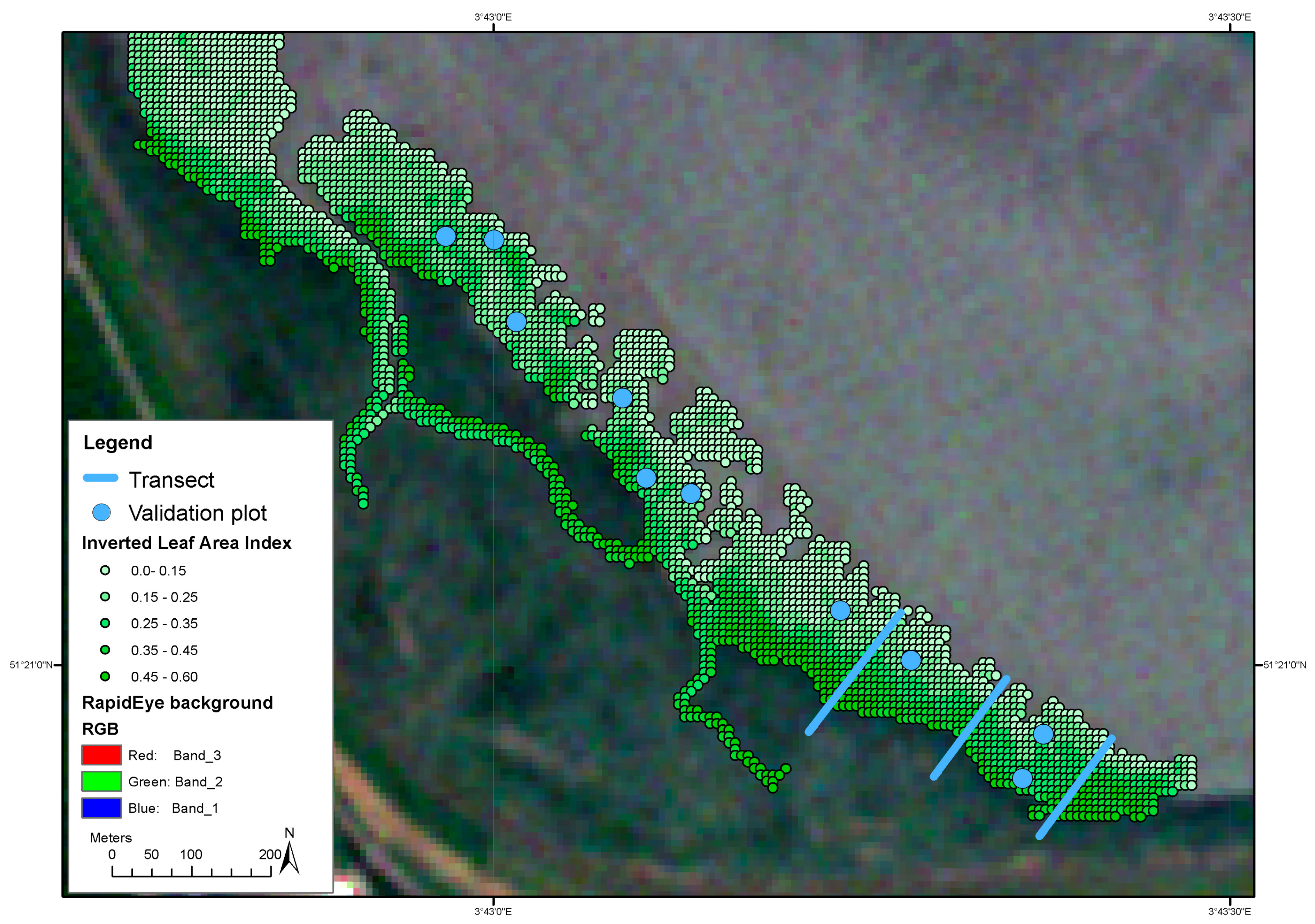
2.8. Application to Spaceborne Data

To test the applicability of the method to spaceborne data, we used a RapidEye satellite image of June 5th, 2015 with a spatial resolution of 5 m. The image was atmospherically corrected using the Second Simulation of a Satellite Signal in the Solar Spectrum (6S) model, which is known to perform well [61]. This atmospheric correction model requires geometrical, atmospherical, sensor, spectral, ground reflectance, and signal input (see Table 2). The atmospheric profile was set to midlatitude summer.
In the RapidEye image, areas dominated by Spartina were selected, the ProSail model was applied to the reselected areas to estimate LAI. The spatial driver information was extracted at the center of every inverted RapidEye pixel. All analyses were performed on 5 × 5 m pixels.
Again, linear regressions were used to compare the different spatial drivers with the estimated LAI (see method in Section 2.4). The correlation between the effects of different drivers was tested with Pearson correlation tests. In addition a multiple linear regression was used to relate the estimated LAI with the spatial drivers in a single test to avoid explaining variation several times. This allowed us to establish the relative importance of each spatial driver.

3. Results

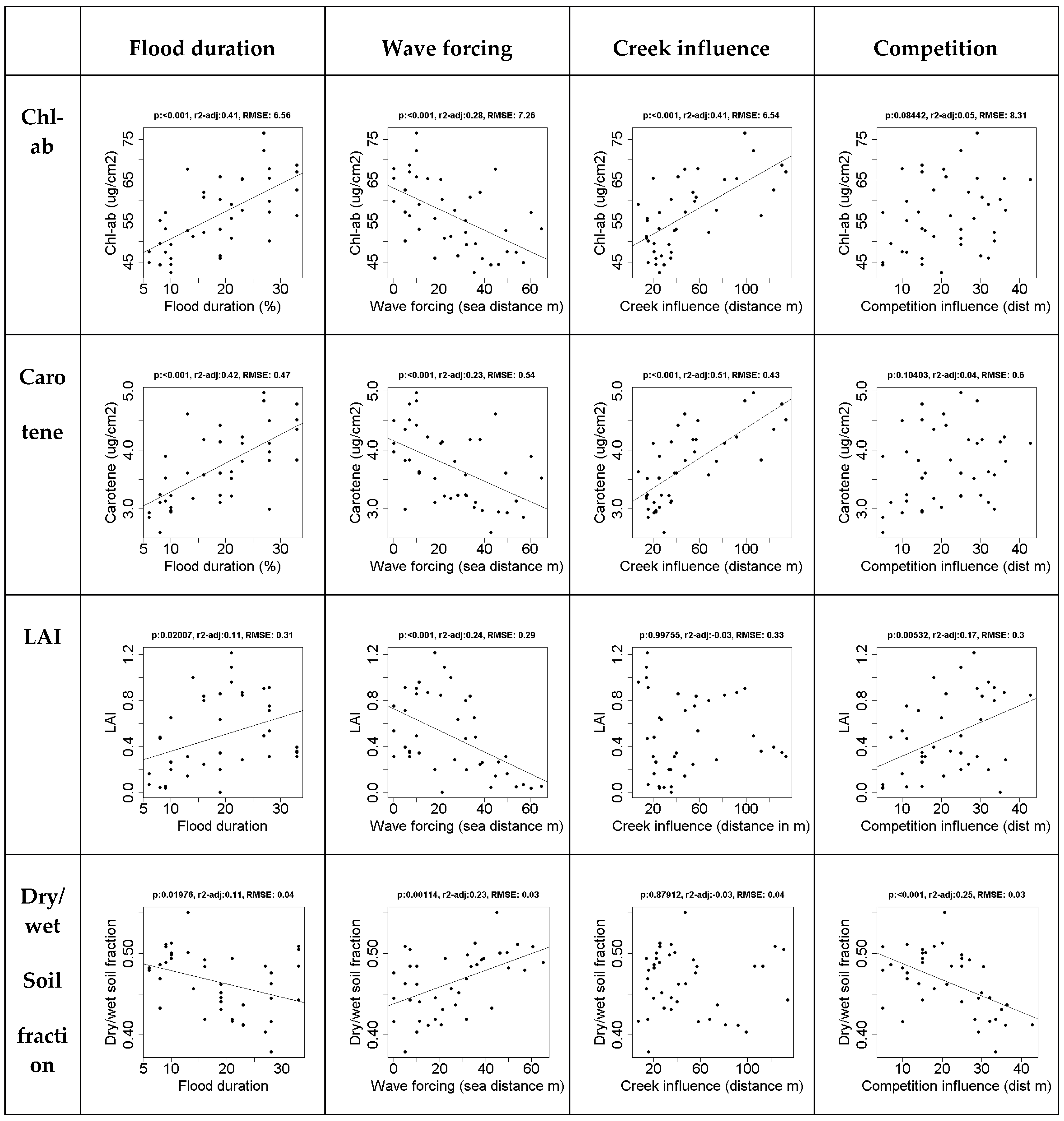
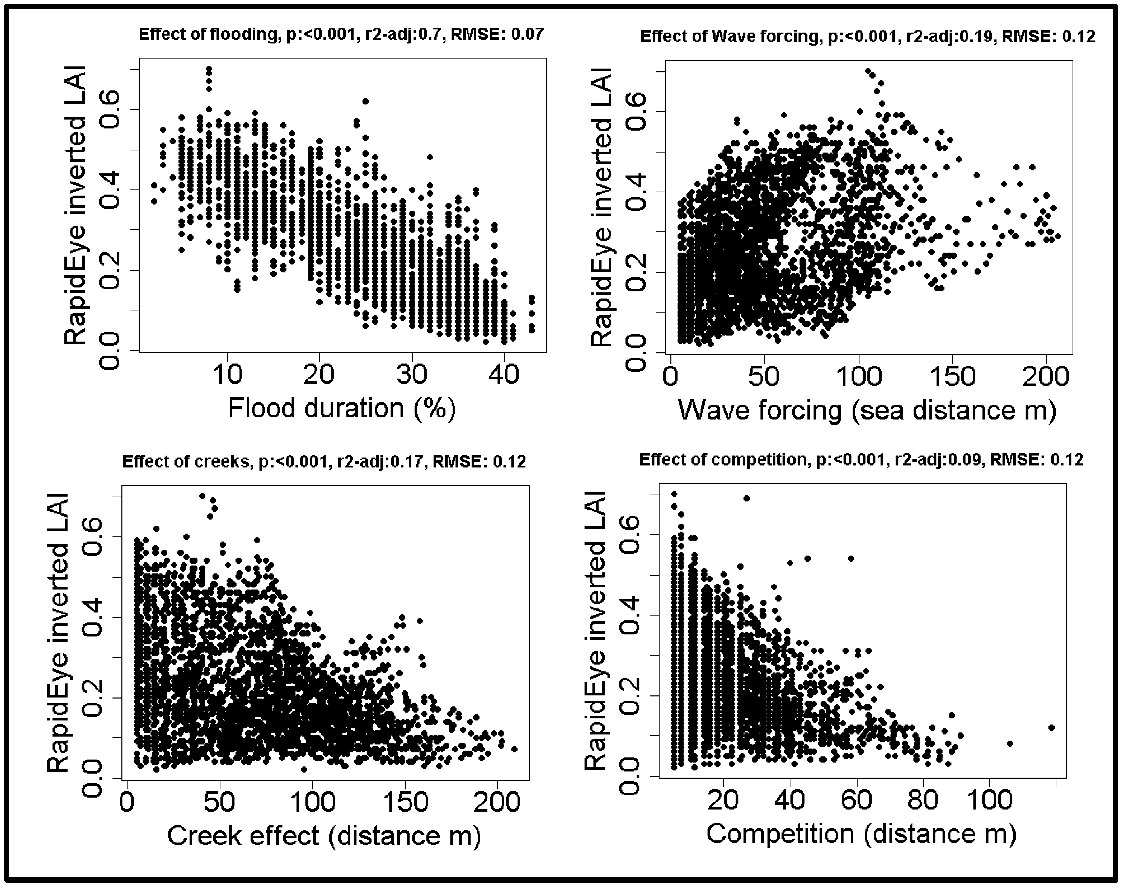
3.1. Effects Spatial Drivers on in situ Vegetation Characteristics

The direct effects of drivers behind spatial variation, i.e., flood duration, wave forcing, competition, and creek influence on in situ measured vegetation properties show that flood duration and wave forcing affected all vegetation characteristics, and their effects were strongest on chlorophyll a+b and carotene content (Figure 1). The level of significance is indicated by p, the r2-adj is the adjusted r2, as reported by the regression functions in R, and RMSE reports the root mean square error.
Competition is strongly correlated with soil moisture content and LAI. Nearness to creeks was only significantly correlated with chlorophyll a+b and carotene content, but this correlation explained over 40% of the variation in both cases.
LAI seems to increase at a higher flood duration. However, a low flood duration only occurs at higher elevation, therefore this value is likely codependent on competition, which only occurs at higher elevations. The highest LAI values do not occur at high flood durations. The overall effect of flood duration on the leaf level is relatively small.

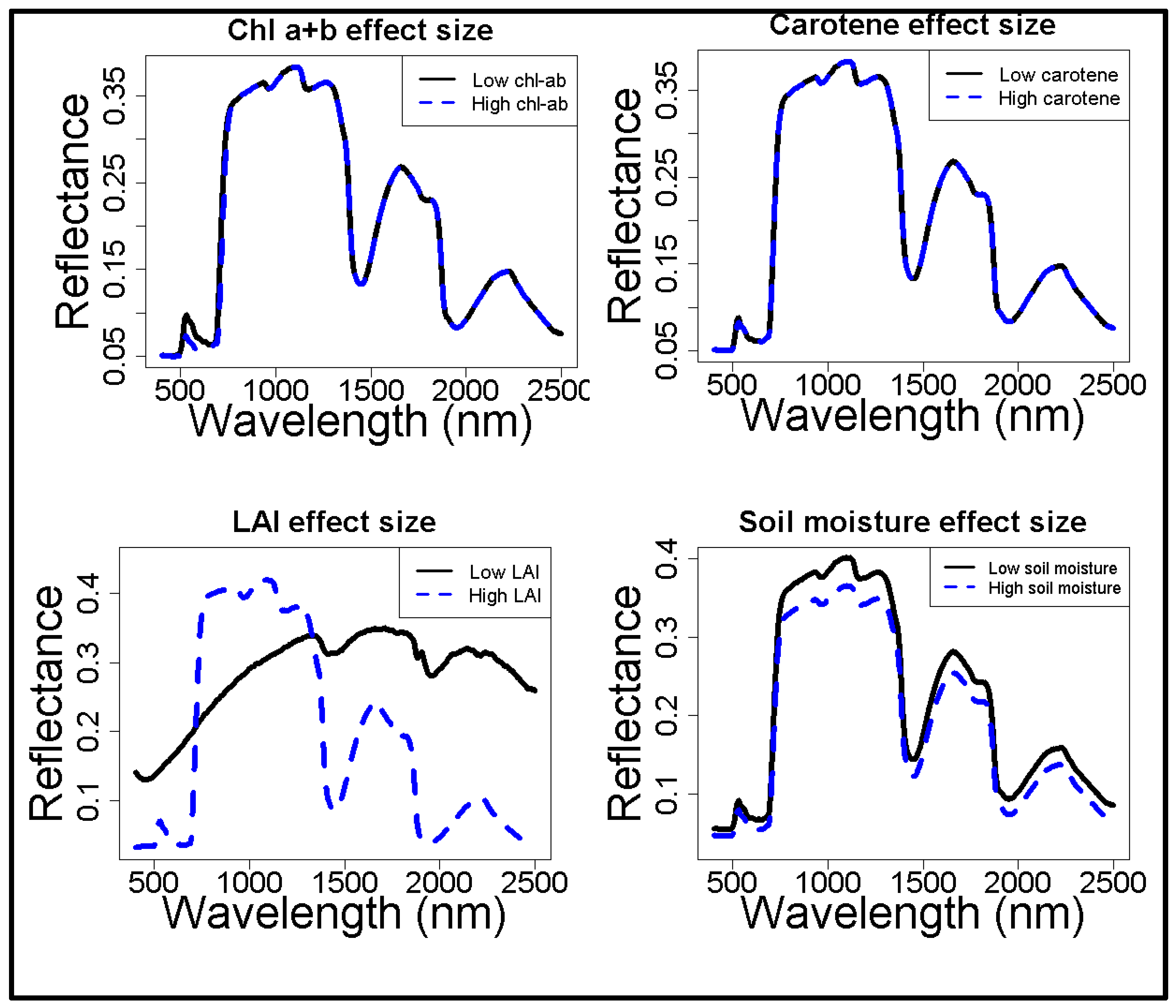
3.2. Effects of Vegetation Characteristics on Reflectance, Modelled Sensitivity

The spectral effects of four of the major model parameters, i.e., chlorophyll a+b, carotene, leaf area index, and soil moisture content, were quantified via a sensitivity analysis on in situ data (Figure 2). The chlorophyll a+b content affects a limited range of wavelengths (i.e., 500 to 750 nm), whereas the effects of carotene on the reflectance spectra were negligible. Hence, the latter was fixed to its average value. LAI and soil moisture content have a large influence on the entire range of the spectrum. LAI shows a decrease of reflectance at higher LAI values, which was expected as higher leaf coverage can absorb more light and hence lower reflectance. As expected, LAI changes the shape of the spectrum, whereas soil moisture content only increases or decreases the entire modelled spectrum. The contribution of leaf level reflectance (as modeled by ‘Prospect’) appears subordinate to the contribution of canopy level reflectance (as modeled by ‘Sail’).

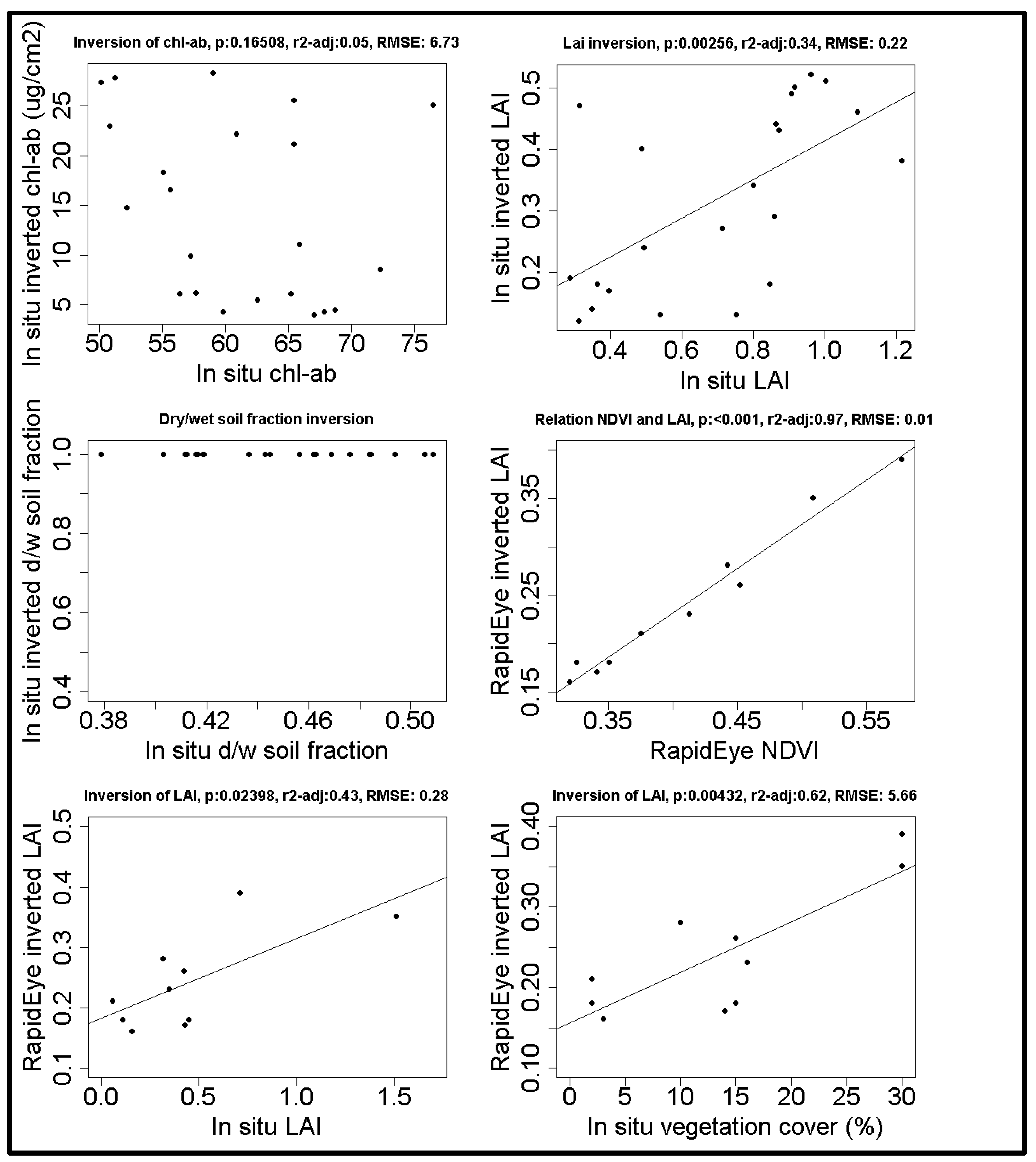
3.3. Model Validation

To validate the model, we compared in situ measurements with estimated values based on the model inversion. The ranges used to construct the LUT’s are shown in Table 3. The model inversion shows that only LAI produces a significant, yet noisy, relationship between in situ measurements and model inversion, in both the calibration and the independent plots (Figure 3). Chlorophyll was poorly estimated, and the soil moisture content was always estimated as completely dry. These were not taken into account any further, but rather fixed at their average values (see Table 1).
The comparison between ProSail and NDVI shows that the estimated LAI is closely related to the NDVI (see Figure 3) (n = 10, p < 0.001, F = 313, r2adj = 0.97). However the ProSail model (n = 10, p = 0.02, F = 7.72, R2adj = 0.4275) performs slightly better than NDVI (n = 10, p = 0.036, F = 6.318, R2adj = 0.3714). Therefore, and for an improved comparability, we used the inverted model to estimate the leaf area index.

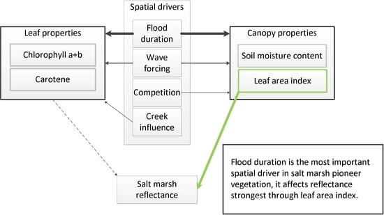
3.4. Large Scale Effect of Spatial Drivers

The inverted model was used to estimate LAI from satellite images; these data clearly show that flood duration has the largest influence on vegetation reflectance, followed by both wave forcing and distance to the nearest creek. Flood duration explains over three times as much variation as any of the other explanatory variables (Figure 4). The data clearly show that a higher flood duration decreases LAI (Figure 5). While lower LAI values occur throughout the salt marsh, high LAI values only occur close to competitors and close to creeks. The wave forcing seems highest at a lower LAI, the lowest wave forcing seems to occur along creeks high in the marsh, where LAI is high, although the relationship is noisy and explains only a limited amount of variation.
The Pearson correlation shows that all spatial drivers are significantly correlated (Table 4). The multiple linear regression analysis supports that flood duration had the largest effect by far (Table 5).
Flood duration explains 70% of the total variation, and clearly shows that higher flood duration decreases leaf area index. This seems contradictory to the effect at leaf level, where the pattern is unclear and explains only 11% of the total variation and the highest leaf area index values is found closer to the water. However, when interpreting these results, it is important to take into account that they are based on a different set of plots, as the leaf level analyses includes all plots, and the large scale analysis only includes plots where Spartina was dominant to avoid mixed pixel effects.

4. Discussion

The aim of this paper was to gain insight into which factors drive spatial patterns in the mono-specific pioneer zone of a salt marsh, and through which vegetation properties these drivers affect reflectance. We found that in spring, in our study area flood duration has by far the largest effect on large scale spatial patterns and is the main mechanism behind these patterns. Flood duration is known to have a large effect on vegetation zonation, [2,26,31,32]. Here, we showed that, in our study area, it is the driving factor behind spatial patterns in the mono-specific pioneer zone in spring. A higher flood duration was found to decrease the leaf area index. Flood duration explained 70% of the total spatial variation in LAI, over three times as much as the effect of wave forcing, which was found to be the second most important driver. Wave forcing is also known to be a shaping feature [36], and our result indicate that it indeed affected LAI. However, wave forcing only explains 19% of the total variation and the relationship appears noisy. The other two drivers behind spatial patterns, competition and creek influence, both show the same pattern: High LAI values only occur at low distances to competitors or creeks, low values occur everywhere. These drivers explain respectively 9% and 17% of the total variation only. At this spatial scale, it is clear that flood duration is most correlated to the differences in reflectance, overshadowing the effects of other factors.
It is important to note that this study is a first step towards understanding how drivers behind spatial patterns affect reflectance of the vegetation of single species and create spatial patterns. We focused on the monospecific pioneer zone of a single salt marsh in spring. Therefore, our results have to be applied to other species and sites with other conditions, before conclusions can be drawn on salt marshes in a broader sense.

4.1. Applicability to Other Vegetation Zones

In this study we focused on the pioneer zone of a salt marsh. Hence, it is possible that in the middle and high marsh other drivers become relatively more important, especially where differences in flood duration become relatively small. In our study, we focused on a single species (Spartina), the pioneer zone was dominated by this species. At higher elevations, other species become more important. Previous research showed that even small differences in flood duration can already cause large differences in vegetation zonation, i.e., yielding different vegetation species or communities [26]. This indicates that this flood duration has an effect even in the middle and high marsh. Additionally, the effect of wave forcing is also most likely to be strongest in the pioneer zone, and competition is known to be an important process throughout salt marshes [2,38,39]. Therefore, it seems unlikely that the large influence of flood duration is only limited to the pioneer zone. However, further study will have to establish its importance in other salt marsh regions, and with species other than Spartina. Another consequence of limiting ourselves to the pioneer zone is that we reduce the effects of competition, as competition is likely to have strong effects near the border between vegetation types. These borders were excluded as they presented mixed pixels that could not be inverted by the model. We therefore recommend future studies into modeling all salt marsh vegetation types in a single model, in order to expand research beyond the pioneer zone and establish the most important spatial drivers for the entire salt marsh.
Our study site is relatively sheltered. In a more exposed site, the balance between wave forcing and flood duration might shift. It seems unlikely that this would affect the relative importance of the other considered drivers (i.e., competition and creeks). In the sheltered pioneer zone, which is relatively important with regard to the ecosystem service provision [62], it was found that flood duration is the most important driver behind spatial patterns.

4.2. ProSail

To establish how flood duration affects reflectance, we used the physical model ProSail. This model combines information on leaf and canopy levels to simulate reflectance spectra. The performed analysis showed that vegetation density and cover, represented by LAI, is the most influential in the reflectance spectra. Therefore, the drivers seem to produce large scale spatial patterns by affecting local values of LAI. LAI is one of the main driving variables and can affect the entire spectrum [12], however, measuring LAI can be challenging [63]. A recent global review of ProSail showed that ProSail is often used to model LAI, however, there are several problems associated with it [12]. The inversion of LAI can strongly depend upon the number of satellite bands used in agricultural situations [64] and can saturate at higher LAI values [12,64]. This saturation occurred around LAI values of 6 [64], which are unlikely to ever occur in European salt marshes. Another problem associated with ProSail in agricultural areas is that at earliest and late growth stages with very low LAI, the background reflectance dominates the spectral signal [12]. This is reported at the earliest growth stages [12], As the measured LAI and the vegetation cover show the soil is not completely covered hence soil reflectance does contribute to the reflectance spectra. The LAI estimate could be improved by including in situ soil spectra in the model.
In this study LAI was estimated with an inversion of the ProSail model, and compared with in situ LAI and cover measurements. This showed a significant relation between modelled and measured LAI and cover, but also indicated the inversion contains significant noise and has a relatively high RMSE.
We found a strong correlation between NDVI and our LAI estimate. NDVI is one of the most often used methods of describing spatial variation in vegetation. The high correlation with NDVI shows that the inverted LAI represent the spatial patterns well. We would caution against using this LAI inversion in an application where the absolute LAI values are of great importance.
This analysis was performed with RapidEye, which has a multispectral satellite sensor with five spectral bands. This satellite constellation is often used for vegetation studies, however the estimation of Leaf Area Index might be improved by using a satellite with more spectral bands. A neural networking approach showed that, for LAI estimations, seven bands is optimal [64]. A better LAI estimate may be obtained with a satellite sensor with both a better spectral and radiometric resolution. RapidEye has a 12-bit digitization with low readout noise [65]. Its dynamic range of 12-bits/pixel is comparable to other broad-band sensors with a similar spatial resolution, such as Pleiades and SPOT 6/7, but is worse than, for example, KompSat and Sentinel-2 [66].
On a large spatial scale the effects of leaf properties (chlorophyll a+b, carotene) could not be detected. The canopy properties (leaf area index and dry/wet soil fraction) largely overwrite the effects of the leaf properties.
ProSail is mainly used in agricultural settings [12,13,67,68,69,70], often used to study chlorophyll [67,71,72]. We used ProSail to simulate the effect of chlorophyll on reflectance at the leaf scale and found that the range of chlorophyll contents among the leaves observed in the study site was not enough to explain large-scale variations in reflectance, suggesting that chlorophyll content of the leaves does not play a major role in large scale spatial patterns in the pioneer zone of salt marshes. It is likely that a wider range of values (e.g., in chlorophyll content of the leaves) will occur when multiple seasons are measured. However, we only studied a single species during a single season (i.e., Spartina anglica during mid spring). As a consequence, the chlorophyll content at the leaf level had very limited variability and so it had a limited effect on reflectance.
In Spartina stands, our analyses showed that LAI estimates are closely related to NDVI values, agreeing with previous literature [73]. This indicates that correlation studies relating biophysical properties directly to a vegetation index are not necessarily improved by using a more complex physical model. In our study, the physical model (ProSail) performed only marginally better than a regular NDVI. The main advantage of using ProSail is that it allows for the distinction between leaf and canopy level effects, and even distinguishes between individual effects. However, for further studies not requiring this level of differentiation, we recommend using simple correlation based on vegetation indices. The slight improvement in performance and understanding is outweighed by the large number of extra input parameters and computation required.

4.3. Effect of Spatial Drivers on Leaf and Canopy Level

In large scale patterns, leaf level biophysics are overwritten by canopy characteristics. However, the leaf characteristics are affected by spatial drivers. Both chlorophyll a+b and carotene contents were strongly affected by the duration of flooding and the influence of creeks. These relations were positive; higher flood duration increases chlorophyll content. As plants that are flooded more often suffer a higher stress, the opposite might be also expected. Decreasing chlorophyll content is a common response to a variety of stressors [74]. Spartina is also known to decrease its chlorophyll when stressed, but the force required to stress a plant differs greatly between Spartina species [75]. It is possible that in our study site Spartina was not stressed by the regular flooding. Plants are able to adapt well to regularly occurring phenomena, such as the day night cycle, and these factors are not considered stressors, but are described as ‘regular acclimation’ [76]. However, our results indicate that biomass is lower when they are flooded more frequently, indicating that they are indeed stressed. This is also indicated by their improved growth when moved higher in the marsh [2]. Another possibility is that the increase in environmental stress reduces light competition, although our data showed that chlorophyll content is not related to competition. Light availability is also codetermined by flood duration, as top leafs are flooded less than the rest of the plant. We tested the chlorophyll content of fully grown leaves near the top of the plant, so it is also possible that these plants allocate more of their chlorophyll production to their highest leaves, as these are flooded least. This will have to be studied further.
Creeks were also found to strongly affect chlorophyll content (a+b and carotene). Creeks are known to affect soil conditions (e.g., carbon and nitrogen content) [41], which could play a role in chlorophyll development. However, many of our plots were >40 m away from a creek, and chlorophyll content is lowest closer to a creek. Chlorophyll content is therefore unlikely to be a largely affected by nutrients provided by creeks. It remains unclear how this spatial driver affects vegetation properties. The position of a creek might be codetermined by an underlying cause also affecting chlorophyll content, or the spatial influence of creeks might be larger than expected.
At the canopy level, we found that LAI and soil moisture content are affected most by wave forcing and competition. In our study area, wave forcing and competition complement each other: high competition only occurs at low wave forcing and vice versa. The Spartina LAI values here presented decreased as competition increased, and correspondingly, also decreased at low wave force levels. A similar pattern is seen in the relation between LAI and flood duration. At low flood duration LAI is low, which corresponds to an increased competition. The highest LAI values occur at intermediate flood duration. This hints towards an optimal growing position, close to the water a high flood duration causes stress, high in the marsh competitors cause stress. This pattern is known in salt marshes [2].
Overall, the effects of spatial drivers are stronger at the leaf level, likely because here biophysical properties are relatively simple and easy to measure. At the canopy level, there is more noise and the effect of spatial drivers becomes less obvious. This is likely because the canopy level has more complex parameters, such as leaf orientation, which are difficult to measure correctly [12]. The larger variation at canopy level is reinforced by the inherit increase in variation that comes with scaling up. The relationships described by the regression models is intended to show how vegetation characteristics respond to spatial drivers, we would therefore argue for great caution when applying them as predictive models.

5. Conclusions

As a first step towards understanding drivers behind spatial patterns in salt marshes, we studied the monospecific (Spartina) pioneer zone of a European salt marsh in spring. We found that the spatial patterns where mainly caused by flood duration, which affects spatial patterns through leaf area index. Flood duration explained over three times as much variation as wave forcing, competition or creek influence. The influence of drivers on spatial patterns seems to be stronger on canopy properties, especially leaf area index, than on leaf characteristics, which play only a minor role. This knowledge is a first step towards improving our capacity to use remote sensing signals as proxies for salt marsh mechanisms. Since simple indices such as NDVI performed nearly as well as physical models in our salt marsh pioneer area, NDVI may be well suited for monitoring these relatively simple systems.

Author Contributions

Conceptualization, B.O., E.P.M. and D.v.d.W.; Data curation, B.O. and E.P.M.; Formal analysis, B.O. and E.P.M.; Funding acquisition, G.P. and D.v.d.W.; Investigation, B.O. and E.P.M.; Methodology, B.O., E.P.M. and D.v.d.W.; Project administration, G.P. and D.v.d.W.; Resources, B.O., E.P.M. and D.v.d.W.; Software, B.O. and E.P.M.; Supervision, T.J. Bouma and D.v.d.W.; Validation, B.O. and E.P.M.; Visualization, B.O.; Writing – original draft, B.O., E.P.M. and D.v.d.W.; Writing – review & editing, B.O., G.P., T.J.B. and D.v.d.W.

Funding

This research received funding from the European Union’s Seventh Framework Programme (Space) under grant agreement no 607131, project FAST (Foreshore Assessment using Space Technology).

Acknowledgments

We acknowledge the support of field assistants Lennart van IJzerloo and Jeroen van Dalen and students who helped collecting the data. In addition we recognize Ben Evans and Iris Möller, who were fundamental to the FAST project, but were not directly involved with this paper.

Conflicts of Interest

The authors declare no conflict of interest.

References

  1. Legendre, P.; Fortin, M.J. Spatial pattern and ecological analysis. Vegetatio 1989, 80, 107–138. [Google Scholar] [CrossRef] [Green Version]
  2. Bertness, M.D.; Ellison, A.M. Determinants of pattern in a New England salt marsh plant community. Ecol. Monogr. 1987, 129–147. [Google Scholar] [CrossRef]
  3. Kéfi, S.; Dakos, V.; Scheffer, M.; Van Nes, E.H.; Rietkerk, M. Early warning signals also precede non-catastrophic transitions. Oikos 2013, 122, 641–648. [Google Scholar] [CrossRef]
  4. van Belzen, J.; van de Koppel, J.; Kirwan, M.L.; van der Wal, D.; Herman, P.M.J.; Dakos, V.; Kéfi, S.; Scheffer, M.; Guntenspergen, G.R.; Bouma, T.J. Vegetation recovery in tidal marshes reveals critical slowing down under increased inundation. Nat. Commun. 2017, 8, ncomms15811. [Google Scholar] [CrossRef] [PubMed]
  5. Marani, M.; Da Lio, C.; D’Alpaos, A. Vegetation engineers marsh morphology through multiple competing stable states. Proc. Natl. Acad. Sci. 2013, 110, 3259–3263. [Google Scholar] [CrossRef] [PubMed] [Green Version]
  6. Samanta, A.; Ganguly, S.; Hashimoto, H.; Devadiga, S.; Vermote, E.; Knyazikhin, Y.; Nemani, R.R.; Myneni, R.B. Amazon forests did not green-up during the 2005 drought. Geophys. Res. Lett. 2010, 37. [Google Scholar] [CrossRef] [Green Version]
  7. Murad, H.; Islam, A. Drought assessment using remote sensing and GIS in north-west region of Bangladesh. In Proceedings of the Proceedings of the 3rd International Conference on Water & Flood Management, Dhaka, Bangladesh, 8–10 January 2011; pp. 797–804. [Google Scholar]
  8. Caccamo, G.; Chisholm, L.A.; Bradstock, R.A.; Puotinen, M.L. Assessing the sensitivity of MODIS to monitor drought in high biomass ecosystems. Remote Sens. Environ. 2011, 115, 2626–2639. [Google Scholar] [CrossRef]
  9. Aldakheel, Y.Y. Assessing NDVI spatial pattern as related to irrigation and soil salinity management in Al-Hassa Oasis, Saudi Arabia. J. indian Soc. Remote Sens. 2011, 39, 171–180. [Google Scholar] [CrossRef]
  10. Lobell, D.B.; Lesch, S.M.; Corwin, D.L.; Ulmer, M.G.; Anderson, K.A.; Potts, D.J.; Doolittle, J.A.; Matos, M.R.; Baltes, M.J. Regional-scale assessment of soil salinity in the Red River Valley using multi-year MODIS EVI and NDVI. J. Environ. Qual. 2010, 39, 35–41. [Google Scholar] [CrossRef] [PubMed]
  11. Belluco, E.; Camuffo, M.; Ferrari, S.; Modenese, L.; Silvestri, S.; Marani, A.; Marani, M. Mapping salt-marsh vegetation by multispectral and hyperspectral remote sensing. Remote Sens. Environ. 2006, 105, 54–67. [Google Scholar] [CrossRef]
  12. Berger, K.; Atzberger, C.; Danner, M.; D’Urso, G.; Mauser, W.; Vuolo, F.; Hank, T. Evaluation of the PROSAIL model capabilities for future hyperspectral model environments: a review study. Remote Sens. 2018, 10, 85. [Google Scholar] [CrossRef]
  13. Tripathi, R.; Sahoo, R.N.; Sehgal, V.K.; Tomar, R.K.; Chakraborty, D.; Nagarajan, S. Inversion of PROSAIL model for retrieval of plant biophysical parameters. J. Indian Soc. Remote Sens. 2012, 40, 19–28. [Google Scholar] [CrossRef]
  14. Jacquemoud, S. Inversion of the PROSPECT+ SAIL canopy reflectance model from AVIRIS equivalent spectra: theoretical study. Remote Sens. Environ. 1993, 44, 281–292. [Google Scholar] [CrossRef]
  15. Bicheron, P.; Leroy, M. A method of biophysical parameter retrieval at global scale by inversion of a vegetation reflectance model. Remote Sens. Environ. 1999, 67, 251–266. [Google Scholar] [CrossRef]
  16. Boesch, D.F.; Turner, R.E. Dependence of fishery species on salt marshes: the role of food and refuge. Estuaries 1984, 7, 460–468. [Google Scholar] [CrossRef]
  17. Deegan, L.A.; Hughes, J.E.; Rountree, R.A. Salt marsh ecosystem support of marine transient species. In Concepts and controversies in tidal marsh ecology; Springer: Berlin/Heidelberg, Germany, 2002; pp. 333–365. ISBN 0792360192. [Google Scholar]
  18. Chmura, G.L. What do we need to assess the sustainability of the tidal salt marsh carbon sink? Ocean Coast. Manag. 2011. [Google Scholar] [CrossRef]
  19. Henderson, F.M.; Lewis, A.J. Radar detection of wetland ecosystems: a review. Int. J. Remote Sens. 2008, 29, 5809–5835. [Google Scholar] [CrossRef] [Green Version]
  20. Möller, I. Quantifying saltmarsh vegetation and its effect on wave height dissipation: Results from a UK East coast saltmarsh. Estuar. Coast. Shelf Sci. 2006, 69, 337–351. [Google Scholar] [CrossRef]
  21. Barbier, E.B.; Koch, E.W.; Silliman, B.R.; Hacker, S.D.; Wolanski, E.; Primavera, J.; Granek, E.F.; Polasky, S.; Aswani, S.; Cramer, L.A. Coastal ecosystem-based management with nonlinear ecological functions and values. Science 2008, 319, 321–323. [Google Scholar] [CrossRef] [PubMed]
  22. Möller, I.; Kudella, M.; Rupprecht, F.; Spencer, T.; Paul, M.; Van Wesenbeeck, B.K.; Wolters, G.; Jensen, K.; Bouma, T.J.; Miranda-Lange, M. Wave attenuation over coastal salt marshes under storm surge conditions. Nat. Geosci. 2014, 7, 727–731. [Google Scholar] [CrossRef]
  23. Rönnbäck, P. The ecological basis for economic value of seafood production supported by mangrove ecosystems. Ecol. Econ. 1999, 29, 235–252. [Google Scholar] [CrossRef]
  24. Jerath, M.; Bhat, M.; Rivera-Monroy, V.H.; Castañeda-Moya, E.; Simard, M.; Twilley, R.R. The role of economic, policy, and ecological factors in estimating the value of carbon stocks in Everglades mangrove forests, South Florida, USA. Environ. Sci. Policy 2016, 66, 160–169. [Google Scholar] [CrossRef]
  25. Rizal, A.; Sahidin, A.; Herawati, H. Economic Value Estimation of Mangrove Ecosystems in Indonesia. Biodivers. Int. J. 2018, 2, 51. [Google Scholar] [CrossRef]
  26. Zedler, J.B.; Callaway, J.C.; Desmond, J.S.; Vivian-Smith, G.; Williams, G.D.; Sullivan, G.; Brewster, A.E.; Bradshaw, B.K. Californian salt-marsh vegetation: an improved model of spatial pattern. Ecosystems 1999, 2, 19–35. [Google Scholar] [CrossRef]
  27. Sanderson, E.W.; Foin, T.C.; Ustin, S.L. A simple empirical model of salt marsh plant spatial distributions with respect to a tidal channel network. Ecol. Modell. 2001, 139, 293–307. [Google Scholar] [CrossRef]
  28. Silvestri, S.; Marani, M. Salt-Marsh Vegetation and Morphology: Basic Physiology, Modelling and Remote Sensing Observations. Ecogeomorphology Tidal Marshes 2004, 5–25. [Google Scholar]
  29. Pettengill, T.M.; Crotty, S.M.; Angelini, C.; Bertness, M.D. A natural history model of New England salt marsh die-off. Oecologia 2018, 186, 621–632. [Google Scholar] [CrossRef] [PubMed]
  30. Moffett, K.B.; Robinson, D.A.; Gorelick, S.M. Relationship of salt marsh vegetation zonation to spatial patterns in soil moisture, salinity, and topography. Ecosystems 2010, 13, 1287–1302. [Google Scholar] [CrossRef]
  31. Silvestri, S.; Defina, A.; Marani, M. Tidal regime, salinity and salt marsh plant zonation. Estuar. Coast. Shelf Sci. 2005, 62, 119–130. [Google Scholar] [CrossRef]
  32. Pennings, S.C.; Callaway, R.M. Salt marsh plant zonation: the relative importance of competition and physical factors. Ecology 1992, 73, 681–690. [Google Scholar] [CrossRef]
  33. Neumeier, U.; Ciavola, P. Flow resistance and associated sedimentary processes in a Spartina maritima salt-marsh. J. Coast. Res. 2004, 435–447. [Google Scholar] [CrossRef]
  34. Bouma, T.J.; De Vries, M.B.; Low, E.; Peralta, G.; Tánczos, I.C.; van de Koppel, J.; Herman, P.M.J. Trade-offs related to ecosystem engineering: A case study on stiffness of emerging macrophytes. Ecology 2005, 86, 2187–2199. [Google Scholar] [CrossRef]
  35. Bouma, T.J.; De Vries, M.B.; Herman, P.M.J. Comparing ecosystem engineering efficiency of two plant species with contrasting growth strategies. Ecology 2010, 91, 2696–2704. [Google Scholar] [CrossRef] [PubMed] [Green Version]
  36. Callaghan, D.P.; Bouma, T.J.; Klaassen, P.; Van der Wal, D.; Stive, M.J.F.F.; Herman, P.M.J.J. Hydrodynamic forcing on salt-marsh development: Distinguishing the relative importance of waves and tidal flows. Estuar. Coast. Shelf Sci. 2010, 89, 73–88. [Google Scholar] [CrossRef]
  37. Fagherazzi, S.; Carniello, L.; D’Alpaos, L.; Defina, A. Critical bifurcation of shallow microtidal landforms in tidal flats and salt marshes. Proc. Natl. Acad. Sci. 2006, 103, 8337–8341. [Google Scholar] [CrossRef] [PubMed] [Green Version]
  38. Bertness, M.D.; Hacker, S.D. Physical stress and positive associations among marsh plants. Am. Nat. 1994, 363–372. [Google Scholar] [CrossRef]
  39. Emery, N.C.; Ewanchuk, P.J.; Bertness, M.D. Competition and salt-marsh plant zonation: stress tolerators may be dominant competitors. Ecology 2001, 82, 2471–2485. [Google Scholar] [CrossRef]
  40. Xin, P.; Li, L.; Barry, D.A. Tidal influence on soil conditions in an intertidal creek-marsh system. Water Resour. Res. 2013. [Google Scholar] [CrossRef]
  41. Zhao, Q.; Bai, J.; Liu, Q.; Lu, Q.; Gao, Z.; Wang, J. Spatial and Seasonal Variations of Soil Carbon and Nitrogen Content and Stock in a Tidal Salt Marsh with Tamarix chinensis, China. Wetlands 2016, 36, 145–152. [Google Scholar] [CrossRef]
  42. Jacquemoud, S.; Baret, F. PROSPECT: A model of leaf optical properties spectra. Remote Sens. Environ. 1990, 34, 75–91. [Google Scholar] [CrossRef]
  43. Van der Wal, D.; Wielemaker-Van den Dool, A.; Herman, P.M.J. Spatial patterns, rates and mechanisms of saltmarsh cycles (Westerschelde, The Netherlands). Estuar. Coast. Shelf Sci. 2008, 76, 357–368. [Google Scholar] [CrossRef]
  44. Van Der Wal, D.; Herman, P.M.J. Regression-based synergy of optical, shortwave infrared and microwave remote sensing for monitoring the grain-size of intertidal sediments. Remote Sens. Environ. 2007, 111, 89–106. [Google Scholar] [CrossRef]
  45. Van Damme, S.; Struyf, E.; Maris, T.; Ysebaert, T.; Dehairs, F.; Tackx, M.; Heip, C.; Meire, P. Spatial and temporal patterns of water quality along the estuarine salinity gradient of the Scheldt estuary (Belgium and The Netherlands): results of an integrated monitoring approach. Hydrobiologia 2005, 540, 29–45. [Google Scholar] [CrossRef]
  46. Wang, H.; Wal, D.; Li, X.; Belzen, J.; Herman, P.M.J.; Hu, Z.; Ge, Z.; Zhang, L.; Bouma, T.J. Zooming in and out: scale-dependence of extrinsic and intrinsic factors affecting salt marsh erosion. J. Geophys. Res. Earth Surf. 2017. [Google Scholar] [CrossRef]
  47. Kromkamp, J.C.; Morris, E.P.; Forster, R.M.; Honeywill, C.; Hagerthey, S.; Paterson, D.M. Relationship of intertidal surface sediment chlorophyll concentration to hyperspectral reflectance and chlorophyll fluorescence. Estuaries Coasts 2006, 29, 183–196. [Google Scholar] [CrossRef]
  48. Van der Wal, D.; Herman, P.M.J.; Forster, R.M.; Ysebaert, T.; Rossi, F.; Knaeps, E.; Plancke, Y.M.G.; Ides, S.J. Distribution and dynamics of intertidal macrobenthos predicted from remote sensing: response to microphytobenthos and environment. Mar. Ecol. Prog. Ser. 2008, 367, 57–72. [Google Scholar] [CrossRef] [Green Version]
  49. Paree, E. Toelichting op de zoute ecotopenkaart Westerschelde 2016 - Biologische monitoring zoute rijkswateren; Rijkswaterstaat Ministerie Infrastructuur en Milieu: The Hague, The Netherlands, 2017; 25p. [Google Scholar]
  50. Tolman, M.E.; Pranger, D.P. Toelichting bij de Vegetatiekartering Westerschelde 2010. Rijkswaterstaat Minist. van verkeer en Waterstaat Delft 2012, 1–114. Available online: http://publicaties.minienm.nl/documenten/toelichting-bij-de-vegetatiekartering-westerschelde-2010-op-basi (accessed on 19 February 2019).
  51. Verhoef, W. Light scattering by leaf layers with application to canopy reflectance modeling: the SAIL model. Remote Sens. Environ. 1984, 16, 125–141. [Google Scholar] [CrossRef]
  52. Jacquemoud, S.; Verhoef, W.; Baret, F.; Bacour, C.; Zarco-Tejada, P.J.; Asner, G.P.; François, C.; Ustin, S.L. PROSPECT+ SAIL models: A review of use for vegetation characterization. Remote Sens. Environ. 2009, 113, S56–S66. [Google Scholar] [CrossRef]
  53. Lehnert L., W.; Meyer, H.; Bendix, J. HSDAR: Manage, analyse and simulate hyperspectral data in R. R package version 0.5.0. (2016). Available online: https://rdrr.io/cran/hsdar/ (accessed on 1 March 2019).
  54. Bowyer, P.; Danson, F.M. Sensitivity of spectral reflectance to variation in live fuel moisture content at leaf and canopy level. Remote Sens. Environ. 2004, 92, 297–308. [Google Scholar] [CrossRef]
  55. Mobasheri, M.R.; Fatemi, S.B. Leaf Equivalent Water Thickness assessment using reflectance at optimum wavelengths. Theor. Exp. Plant Physiol. 2013, 25, 196–202. [Google Scholar] [CrossRef] [Green Version]
  56. Beleites, C.; Sergo, V. HyperSpec: a package to handle hyperspectral data sets in R’, R package version 0.98-20150304. Available online: http://hyperspec.r-forge.r-project.org (accessed on 1 August 2017).
  57. Jensen, J.R.; Coombs, C.; Porter, D.; Jones, B.; Schill, S.; White, D. Extraction of smooth cordgrass (Spartina alterniflora) biomass and leaf area index parameters from high resolution imagery. Geocarto Int. 1998, 13, 25–34. [Google Scholar] [CrossRef]
  58. Van der Meijden, R. Heukels’ Flora van Nederland 22e druk; Wolter-Noordhof: Groningen, The Netherlands, 1996. [Google Scholar]
  59. Morris, J.T. Modelling light distribution within the canopy of the marsh grass Spartina alterniflora as a function of canopy biomass and solar angle. Agric. For. Meteorol. 1989, 46, 349–361. [Google Scholar] [CrossRef]
  60. Kruse, F.A.; Lefkoff, A.B.; Boardman, J.W.; Heidebrecht, K.B.; Shapiro, A.T.; Barloon, P.J.; Goetz, A.F.H. The spectral image processing system (SIPS)—interactive visualization and analysis of imaging spectrometer data. Remote Sens. Environ. 1993, 44, 145–163. [Google Scholar] [CrossRef]
  61. Kotchenova, S.Y.; Vermote, E.F. Validation of a vector version of the 6S radiative transfer code for atmospheric correction of satellite data Part II Homogeneous Lambertian and anisotropic surfaces. Appl. Opt. 2007, 46, 4455. [Google Scholar] [CrossRef] [PubMed] [Green Version]
  62. Feagin, R.A.; Martinez, M.L.; Mendoza-Gonzalez, G.; Costanza, R. Salt marsh zonal migration and ecosystem service change in response to global sea level rise: a case study from an urban region. Ecol. Soc. 2010, 15. [Google Scholar] [CrossRef]
  63. Zheng, G.; Moskal, L.M. Retrieving leaf area index (LAI) using remote sensing: theories, methods and sensors. Sensors 2009, 9, 2719–2745. [Google Scholar] [CrossRef] [PubMed]
  64. Verger, A.; Baret, F.; Camacho, F. Optimal modalities for radiative transfer-neural network estimation of canopy biophysical characteristics: Evaluation over an agricultural area with CHRIS/PROBA observations. Remote Sens. Environ. 2011, 115, 415–426. [Google Scholar] [CrossRef]
  65. Tyc, G.; Tulip, J.; Schulten, D.; Krischke, M.; Oxfort, M. The RapidEye mission design. Acta Astronaut. 2005, 56, 213–219. [Google Scholar] [CrossRef]
  66. Sozzi, M.; Marinello, F.; Pezzuolo, A.; Sartori, L. Benchmark of Satellites Image Services for Precision Agricultural use. In Proceedings of the AgEng Conference, Wageningen, The Netherlands, 8–11 July 2018. [Google Scholar]
  67. Botha, E.J.; Leblon, B.; Zebarth, B.; Watmough, J. Non-destructive estimation of potato leaf chlorophyll from canopy hyperspectral reflectance using the inverted PROSAIL model. Int. J. Appl. Earth Obs. Geoinf. 2007, 9, 360–374. [Google Scholar] [CrossRef]
  68. Tripathi, R.; Sahoo, R.N.; Sehgal, V.K.; Gupta, V.K.; Bhattacharya, B.B.K.; Gupta, K.; Bhattacharya, B.B.K. Remote Sensing Derived Composite Vegetation Health Index Through Inversion of Prosail for Monitoring of Wheat Growth in Trans Gangetic Plains of India. ISPRS Arch. XXXVIII-8/W3 Work. Proc. Impact Clim. Chang. Agric. 2009, 319–325. [Google Scholar]
  69. Duan, S.-B.; Li, Z.-L.; Wu, H.; Tang, B.-H.; Ma, L.; Zhao, E.; Li, C. Inversion of the PROSAIL model to estimate leaf area index of maize, potato, and sunflower fields from unmanned aerial vehicle hyperspectral data. Int. J. Appl. Earth Obs. Geoinf. 2014, 26, 12–20. [Google Scholar] [CrossRef]
  70. Si, Y.; Schlerf, M.; Zurita-Milla, R.; Skidmore, A.; Wang, T. Mapping spatio-temporal variation of grassland quantity and quality using MERIS data and the PROSAIL model. Remote Sens. Environ. 2012, 121, 415–425. [Google Scholar] [CrossRef]
  71. Li, Z.; Jin, X.; Wang, J.; Yang, G.; Nie, C.; Xu, X.; Feng, H. Estimating winter wheat (Triticum aestivum) LAI and leaf chlorophyll content from canopy reflectance data by integrating agronomic prior knowledge with the PROSAIL model. Int. J. Remote Sens. 2015, 36, 2634–2653. [Google Scholar] [CrossRef]
  72. Kooistra, L.; Clevers, J.G.P.W. Estimating potato leaf chlorophyll content using ratio vegetation indices. Remote Sens. Lett. 2016, 7, 611–620. [Google Scholar] [CrossRef] [Green Version]
  73. Kearney, M.S.; Stutzer, D.; Turpie, K.; Stevenson, J.C. The effects of tidal inundation on the reflectance characteristics of coastal marsh vegetation. J. Coast. Res. 2009, 1177–1186. [Google Scholar] [CrossRef]
  74. Carter, G.A.; Knapp, A.K. Leaf optical properties in higher plants: linking spectral characteristics to stress and chlorophyll concentration. Am. J. Bot. 2001, 88, 677–684. [Google Scholar] [CrossRef] [PubMed] [Green Version]
  75. Castillo, J.M.; Fernández-Baco, L.; Castellanos, E.M.; Luque, C.J.; Figueroa, M.E.; Davy, A.J. Lower limits of Spartina densiflora and S. maritima in a Mediterranean salt marsh determined by different ecophysiological tolerances. J. Ecol. 2000, 88, 801–812. [Google Scholar] [CrossRef]
  76. Lichtenthaler, H.K. Vegetation stress: an introduction to the stress concept in plants. J. Plant Physiol. 1996, 148, 4–14. [Google Scholar] [CrossRef]
Figure 1. The effect of spatial drivers on in situ vegetation properties. The leaf properties (chl-ab and carotene) are strongly affected by flood duration and creek formation. The canopy properties (LAI and the dry/wet soil fraction (1-soil moisture content)), are affected by flood duration, wave forcing and competition. Regression lines are shown for significant relationships: p < 0.05).
Remotesensing 11 00511 g001
Figure 2. The effect of in situ observed ranges in vegetation properties on surface reflectance, based on simulations with ProSail. Surface reflectance is a fraction. The canopy properties (LAI and soil moisture content) have a much larger influence on reflectance than the leaf properties (Chlorophyll a+b and carotene).
Remotesensing 11 00511 g002
Figure 3. The first three graphs show the relation between in situ measurements and the model inversion of in situ spectra. The fourth graph shows the relation between the LAI inversion and NDVI both based on satellite spectra. The final two graphs show the model inversion of satellite spectra with in situ measurements of LAI and vegetation cover. Regression lines are shown for significant relationships p < 0.05).
Remotesensing 11 00511 g003
Figure 4. The large scale effects of the spatial drivers on salt marshes: relationships between drivers and Leaf Area Index (LAI) obtained from inversion of RapidEye satellite images.
Remotesensing 11 00511 g004
Figure 5. Spatial distribution of Leaf Area Index (LAI) estimated from the inversion of the ProSail model applied to a Rapid Eye image of June 5th 2015.
Remotesensing 11 00511 g005
Table 1. ProSail model parameters. The parameter abbreviation is the abbreviation used in HSDAR for the model parameter. The mean value is the average value of the in situ measurements, fixed means it is not derived from in situ measurements. The in situ range describes the range of values (minimum-maximum) that occurred, and were used to simulate their effect on reflectance.
ModelParameter NameModel AbbreviationMean ValueIn Situ RangeSource
ProspectStructure parameterNFixed (1.5)FixedFitted +
[42]
Chlorophyll a+b contentCab (µg/cm2)56.442.4–76.5Chl samples
Carotenoid contentCar (µg/cm2)3.4212.398–4.579Chl samples
Brown pigment contentCbrownN.A.N.A.-
Equivalent water thicknessCw (cm)Fixed (0.0198)Fixedleaf samples
Dry matter contentCm (g/cm2)Fixed (0.0092)FixedLeaf samples
SailDry/Wet soil fraction
(=1- soil moisture content)
pSoil0.53400.4496–0.6214Soil samples
Leaf area indexLAI0.7060.003-1.215[57] +
samples
Type of leaf angle distributionLidfFixed(1,0)Fixed[59]
Hotspot parameterhspotN.A.N.A.-
Solar zenith angleTts (°)N.A.N.A.From timestamp
Observer zenith angleTto (°)N.A.N.A.Always 0
Relative azimuth anglePsi (°)N.A.N.A.From timestamp
Table 2. 6S atmospheric correction model parameters used for the RapidEye atmospheric correction.
ParameterSetting
Month06, from satellite image
Day05, from satellite image
Solar zentih angle (deg)28.91, from satellite image
Solar azimuth angle (deg)171.91, rom satellite image
Sensor zenith angle (deg)12.79, from satellite image
Sensor azimuth angle (deg)281.32, from satellite image
Atmospheric profileMid latitude summer/winter, here summer
Aerosol profileMaritime
Target altitudeSea level
Sensor altitudeSatellite level
Spectral conditionsRapidEye gain, band 1-5
Ground reflectanceHomogeneous surface
Directional effectsNo directional effects
Input ground reflectanceMean spectral value
Atmospheric correction modeAtmospheric correction with Lambertian assumption
Atmospheric correction target0, Reflectance
Table 3. Model inversion look up table properties. LAI: leaf area index; Chl-ab: Chlorophyll a+b content; pSoil: dry/wet soil fraction (=1-soil moisture content).
ParameterMinimumMaximumStepsize
LAI0.00130.01
Chl-ab (µg/cm2)11000.1
pSoil0.110.001
Table 4. The spatial driver correlation coefficients, all spatial drivers were significantly correlated with p values < 0.001.
.Flood DurationWave ForcingCreek InfluenceCompetition
Flood duration1.00−0.440.550.41
Wave forcing−0.441.00−0.30−0.08
Creek influence0.55−0.301.000.41
Competition0.41−0.080.411.00
Table 5. The contribution to the t value in the multiple-regression model relating spatial drivers with leaf area index.
Spatial DriverAbsolute Contribution to t-ValueCoefficient
Flood Duration67.743−0.01078
Wave Forcing9.1240.00033
Creek Influence2.3210.00007
Competition0.9000.00007

