Article

Weighted Spatial Pyramid Matching Collaborative Representation for Remote-Sensing-Image Scene Classification

1
College of Information and Control Engineering, China University of Petroleum (Huadong), No. 66 Changjiang Road West, Huangdao District, Qingdao 266580, China
2
Shandong Provincial Key Laboratory of Computer Networks, Shandong Computer Science Center (National Supercomputer Center in Jinan), Qilu University of Technology (Shandong Academy of Sciences), Fourth Floor, Block B, Yinhe Building, No. 2008 Xinluo Street, Jinan High-Tech Zone, Jinan 250101, China
*
Author to whom correspondence should be addressed.
Submission received: 1 January 2019 / Revised: 25 February 2019 / Accepted: 25 February 2019 / Published: 4 March 2019

Abstract

:
At present, nonparametric subspace classifiers, such as collaborative representation-based classification (CRC) and sparse representation-based classification (SRC), are widely used in many pattern-classification and -recognition tasks. Meanwhile, the spatial pyramid matching (SPM) scheme, which considers spatial information in representing the image, is efficient for image classification. However, for SPM, the weights to evaluate the representation of different subregions are fixed. In this paper, we first introduce the spatial pyramid matching scheme to remote-sensing (RS)-image scene-classification tasks to improve performance. Then, we propose a weighted spatial pyramid matching collaborative-representation-based classification method, combining the CRC method with the weighted spatial pyramid matching scheme. The proposed method is capable of learning the weights of different subregions in representing an image. Finally, extensive experiments on several benchmark remote-sensing-image datasets were conducted and clearly demonstrate the superior performance of our proposed algorithm when compared with state-of-the-art approaches.

1. Introduction

Remote-sensing technology is a kind of high and new technology for air to ground observation, whose primary use is military. However, with the development of economy and the improvement of living standard, it has been gradually used in civil field. By observing the ground at high altitude, the ground object information is obtained and analyzed systematically. Remote-sensing (RS) images are widely used for land cover classification, target identification and thematic mapping from local to global scales owing to its technical advantages such as multi-resolution, wide coverage, repeatable observation and multi/hyperspectral-spectral records. In view that the remote-sensing image tagging samples quantity is less, the traditional image classification method is also suitable for remote-sensing image classification task, such as image feature representation algorithm and small sample classification algorithm.
As a core problem in image-related applications, image-feature representation [1,2] exhibits a trend of transference from handcrafted to learning-based methods. Specifically, most of the early literature is based on handcrafted features. The most classical method is the bag-of-visual-words (BoVW) [3] model. It is built with a histogram of vector-quantized local features and lacks the spatial distribution of local features in the image space. Then, sparse coding [4] was reported to outperform BoVW in this area. Sparse coding permits a linear combination of a small number of codewords, while in BoVW, one local feature corresponds to only one codeword. Sparse coding also lacks the spatial orders of local features. Handcrafted features are limited in their ability to extract robust and transferable feature representation for image scene classification, and ignore many effective cues hiding in the image. In 2006, Hinton [5] pointed out that deep neural networks could learn more profound and essential features of objects of interest, which led to tremendous performance enhancement. After that, many attempts have been made to utilize deep-learning methods to feature learning in remote-sensing images. As one of the most popular deep-learning models in image processing, convolutional neural networks (CNNs) currently dominate the computer-vision literature, achieving state-of-the-art performance in almost every topic to which they are applied.
Lazebnik [6] introduced the spatial pyramid matching (SPM) model to add spatial information of local features to the BoVW model. The proposed method combines together subregion representation. The weights to evaluate the representation of the different subregions are fixed. The SPM model achieved excellent performance for image classification. Therefore, many studies have attempted to embed the spatial orders of local features into BoVW (e.g., Reference [7]). To embed spatial orders into sparse codes, Reference [8] considered a pair of spatially close features as a new local feature followed by sparse coding. BoVW and sparse codes are the sparse representations of the distribution of the local descriptors in the feature space. Dense representation of the distribution has been studied. Reference [9] proposed the Global Gaussian (GG) approach that estimates distribution as a Gaussian distribution and builds the feature by arranging the elements of the mean and covariance of the Gaussian. Similarly, Reference [10], which is a general GG form, proposed to embed local spatial information into a feature by calculating the local autocorrelations of any local features. In spatial pooling, Spatial Pyramid Representation (SPR) [6] is popular for encoding the spatial distribution of local features. SPM with BoVW have been remarkably successful in terms of both scene and object recognition. As for sparse codes, state-of-the-art variants of the spatial pyramid model with linear SVMs work surprisingly well. The variations of sparse codes [11] also utilize SPM.
Another core problem is to construct a visual classifier. Visual-classifier design is a fundamental issue in computer vision. Recently, representation-residual-based classifiers have attracted more attention due to the emerging paradigm of compressed sensing (CS). Representation-residual-based classifiers first obtained the representation of the test sample, and then measured the residual error from the training samples of each class. Zhang et al. [12] proposed the collaborative representation-based classification (CRC) algorithm by using collaborative representation ( 2 norm regularizer). Many researchers from the field of remote sensing are attracted by the superior performance of CRC. Li et al. [13] proposed a joint collaborative-representation (CR) classification method that uses several complementary features to represent an image, including spectral value and spectral gradient features, Gabor texture features, and DMP features. In Reference [14], Liu et al. introduced a hybrid collaborative representation with a kernels-based classification method (Hybrid-KCRC) that combined collaborative representation with class-specific representation, and improved classification rate in RS image classification.
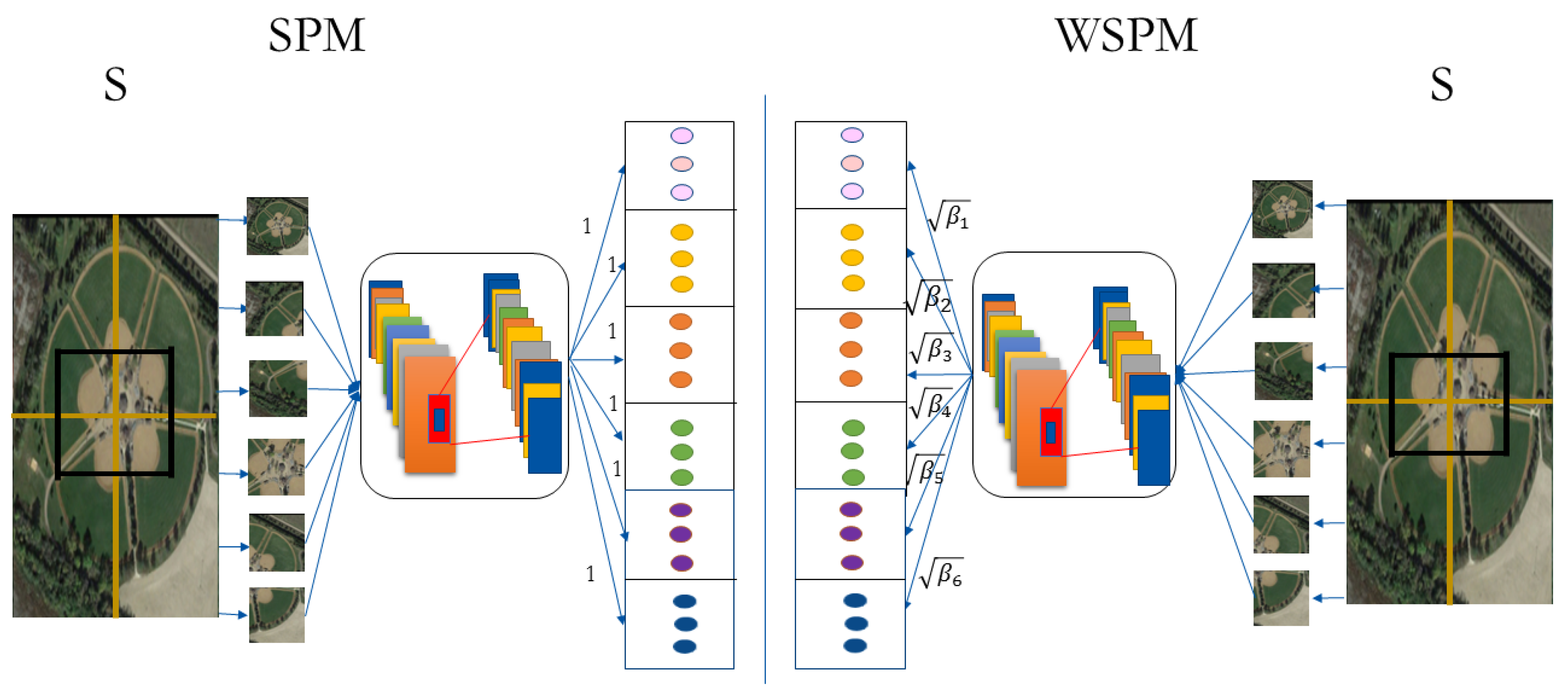
In this paper, we introduce a weighted spatial pyramid matching collaborative representation based classification (WSPM-CRC) method. The proposed method is capable of improving the performance of classifying remote-sensing images by embedding spatial pyramid matching to CRC. Moreover, we also combined the CRC method with the weighted spatial pyramid matching approach to learn the weights of different subregions in representing an image to further enhance classification performance. The scheme of our proposed method is listed in Figure 1. Our work’s main focuses are threefold.
  • We introduce a spatial pyramid matching collaborative representation based classification method that embeds spatial pyramid matching to CRC.
  • To improve conventional spatial pyramid matching, where weights to evaluate the representation of different subregions are fixed, we learn the weights of different subregions.
  • The proposed spatial pyramid matching collaborative representation based classification method was evaluated on four benchmark remote-sensing-image datasets, and achieved state-of-the-art performance.
The rest of the paper is organized as follows. Section 2 overviews several classical visual-recognition algorithms and proposes our spatial pyramid matching collaborative representation based classification. Then, experiment results and analysis are shown in Section 3. Discussion about the experiment results and the proposed method are outlined in Section 4. Finally, conclusions are drawn in Section 5.

2. Proposed Method

In this section, we review related work about CRC. Then, we introduce work about SPM. Finally, we focus on introducing the WSPM.

2.1. CRC Overview

Zhang et al. [12] proposed CRC, for which all training samples are concatenated together as the base vectors to form a subspace, and the test sample is described in the subspace. To be specific, given training samples X = [ X 1 , X 2 , , X C ] R D × N , X c R D × N c represents the training samples from the c t h class, C represents the number of classes, N c represents the number of training samples in the c t h class ( N = c = 1 C N c ), and D represents the sample dimensions. Suppose that y R D × 1 is a test sample, the objective function of CRC is as follows:
f ( s ) = y X s 2 2 + η s 2 2 = k y , y 2 k y , X s + s T k X , X + η I s
Here, k y , y = < y , y > = y T y , k y , X = < y , X > = y T X , k X , X = < X , X > = X T X , η is the regularization parameter to control the tradeoff between fitting goodness and collaborative term (i.e., multiple entries in X participating in representing the test samples). The role of the regularization term is twofold. First, compared with no penalty term, 2 norm stabilizesthe least-squares solution because matrix X may not be full-rank. Second, it introduces a certain amount of “sparsity” to collaborative representation s ^ , and indicates that it is the collaborative representation but not the 1 norm sparsity that makes sparsity powerful for classification. Collaborative-representation-based classification effectively utilizes all training samples for visual recognition, and the objective function of CRC has analytic solutions.

2.2. Spatial Pyramid Matching Model

Svetlana Lazebnik et al. [
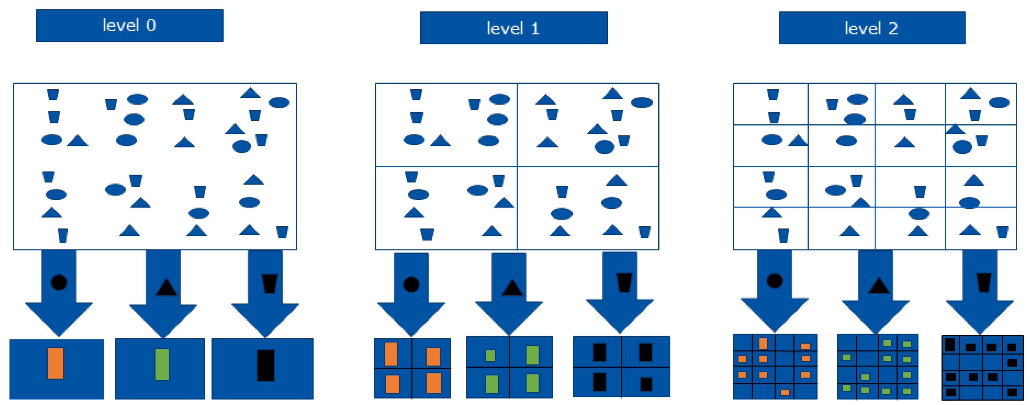
6] proposed the spatial pyramid matching algorithm to compensate for the lack of spatial information in representing an image. The SPM scheme is shown in Figure 2. The image can be represented by three levels. At each level, the image is split into 1, 4, 16 segments. For each subimage, the feature is independently extracted. All features are concatenated to form a feature vector to describe the image. In this paper, we split the image into two levels. For each level, the image is split into 1 and 5 segments (left-upper, left-lower, right-upper, right-lower, center) as shown in Figure 1. Assume x = [ ( x 1 ) T , ( x 2 ) T , , ( x 6 ) T ] T R D × 1 as the feature extracted from an image. The inner product of two image features x and y can be expressed as follows:
< x , y > = k ( x , y ) = m = 1 M k ( x m , y m )
where M = 6 . The SPM model considers that each subimage equally contributes to represent the image. The superior performance of visual recognition is often achieved with the spatial pyramid method, which is to obtain spatial information of images by the statistical distribution of image-feature points at different resolutions. The image is divided into gradually fine grid sequences at all levels of the pyramid. However, the weights to evaluate the representation of different features are fixed.

2.3. Weighted Spatial Pyramid Matching Collaborative Representation

In this paper, we propose the weighted spatial pyramid matching collaborative representation based classification method to learn the weights of different features in representing an image. The weight of each subregion can be learned to achieve superior performance. We assume that x = [ β 1 ( x 1 ) T , β 2 ( x 2 ) T , , β m ( x 6 ) T ] T R D × 1 is the weighted feature extracted from an image. Then, the mode of weighted spatial pyramid matching is as follows:
< x , y > = k x , y = m = 1 M β m k x m , y m s . t . m = 1 M β m 2 = 1
Here, we take both strategies ( m = 1 M β m 2 = 1 and m = 1 M β m = 1 ) into consideration, and both strategies are popular. m = 1 M β m 2 = 1 is adopted because the objective function with m = 1 M β m 2 = 1 constraint is easier to solve.
The objective function of our proposed weighted spatial pyramid matching collaborative representation is as follows:
f s , β = k y , y 2 k y , X s + s T k X , X + η I s s . t . k y , y = m = 1 M β m k y m , y m k y , X = m = 1 M β m k y m , X m k X , X = m = 1 M β m k X m , X m        m = 1 M β m 2 = 1

2.4. Optimization of Objective Function

To optimize Equation (4), it can be transformed as follows:
f s , β = m = 1 M β m k y m , y m 2 m = 1 M β m k y m , X m s + s T m = 1 M β m k X m , X m + η I s s . t . m = 1 M β m 2 = 1
When β m is fixed, the partial derivative of f s , β to s is
f s , β s = 2 m = 1 M β m k y m , X m + 2 m = 1 M β m k X m , X m + η I s
Let f s , β s = 0 , we can obtain the value of s,
s = m = 1 M β m k X m , X m + η I 1 m = 1 M β m k y m , X m
With a fixed s, to optimize objective Equation (5), a Lagrange multiplier was adopted.
g λ , β = f s , β + λ 1 m = 1 M β m 2
To optimize Equation (8), it can be transformed as follows:
g λ , β = m = 1 M β m k y m , y m 2 m = 1 M β m k y m , X m s + s T m = 1 M β m k X m , X m + η I s + λ 1 m = 1 M β m 2
The partial derivative of g λ , β to β m is
g λ , β β m = k y m , y m 2 k y m , X m s + s T k X m , X m s 2 λ β m
The partial derivative of g λ , β to λ is
g λ , β λ = 1 m = 1 M β m 2
Let g λ , β β m be 0; the value of β m with unknown parameter λ is as follows:
β m = k y m , y m 2 k y m , X m s + s T k X m , X m s 2 λ
Let g λ , β λ be 0; the value of β m can be obtained.
β m = k y m , y m 2 k y m , X m s + s T k X m , X m s m = 1 M k y m , y m 2 k y m , X m s + s T k X m , X m s 2

2.5. Weighted Spatial Pyramid Matching Collaborative Representation Based Classification

After obtaining collaborative code s, the weighted spatial pyramid matching collaborative representation based classification is to find the minimum value of the residual error for each class:
i d ( y ) = arg min c y X c s c 2 2
where, X c represents features in the c t h class. i d ( y ) is the label of the testing sample, and y belongs to the class that has minimal residual error. The learned weights hinges on a well-known idea: the reweighting scheme and the latter were used to learn Bayesian networks [15]. The procedure of weighted spatial pyramid matching collaborative representation based classification is shown in Algorithm 1.
Algorithm 1: Algorithm for spatial pyramid matching collaborative representation based classification.
Require: Training samples X R D × N , η , and test sample y
   1:  Initial β and s
   2:  Update s by Equation (7)
   3:  Update β by Equation (12)
   4:  Go back to update s and β until the condition of convergence is satisfied
   5:  for c = 1 ; c C ; c + + do
   6:   Code y with the weighted spatial pyramid matching collaborative representation algorithm.
   7:   Compute the residuals e c ( y ) = y X c s c 2 2
   8:  end for
   9:   i d ( y ) = arg m i n c e c
 10:  return i d ( y )

3. Experiment Results

In this section, we show our experiment results on four remote-sensing-image datasets. To illustrate the significance of our method, we compared it with several state-of-the-art methods. In the following section, we first introduce the experiment settings. Then, we illustrate the experiment results on each aerial-image dataset.

3.1. Experiment Settings

To evaluate the effectiveness of the proposed SPM-CRC and WSPM-CRC, we applied it to the RSSCN7 [16], UC Merced Land Use [17], WHU-RS19 [18], and AID datasets [
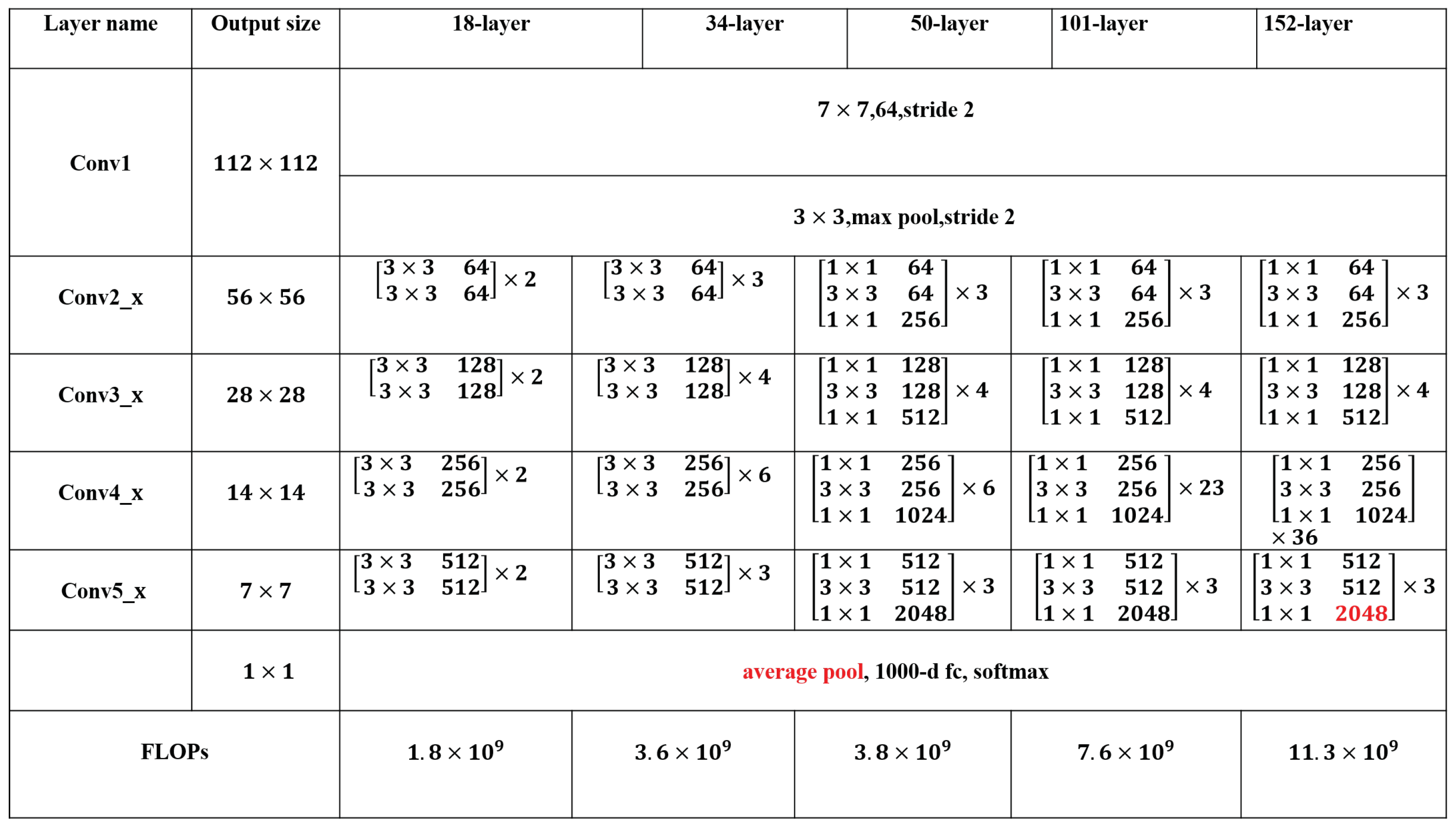
19]. For all datasets, we used two pretrained CNN models, i.e., ResNet [
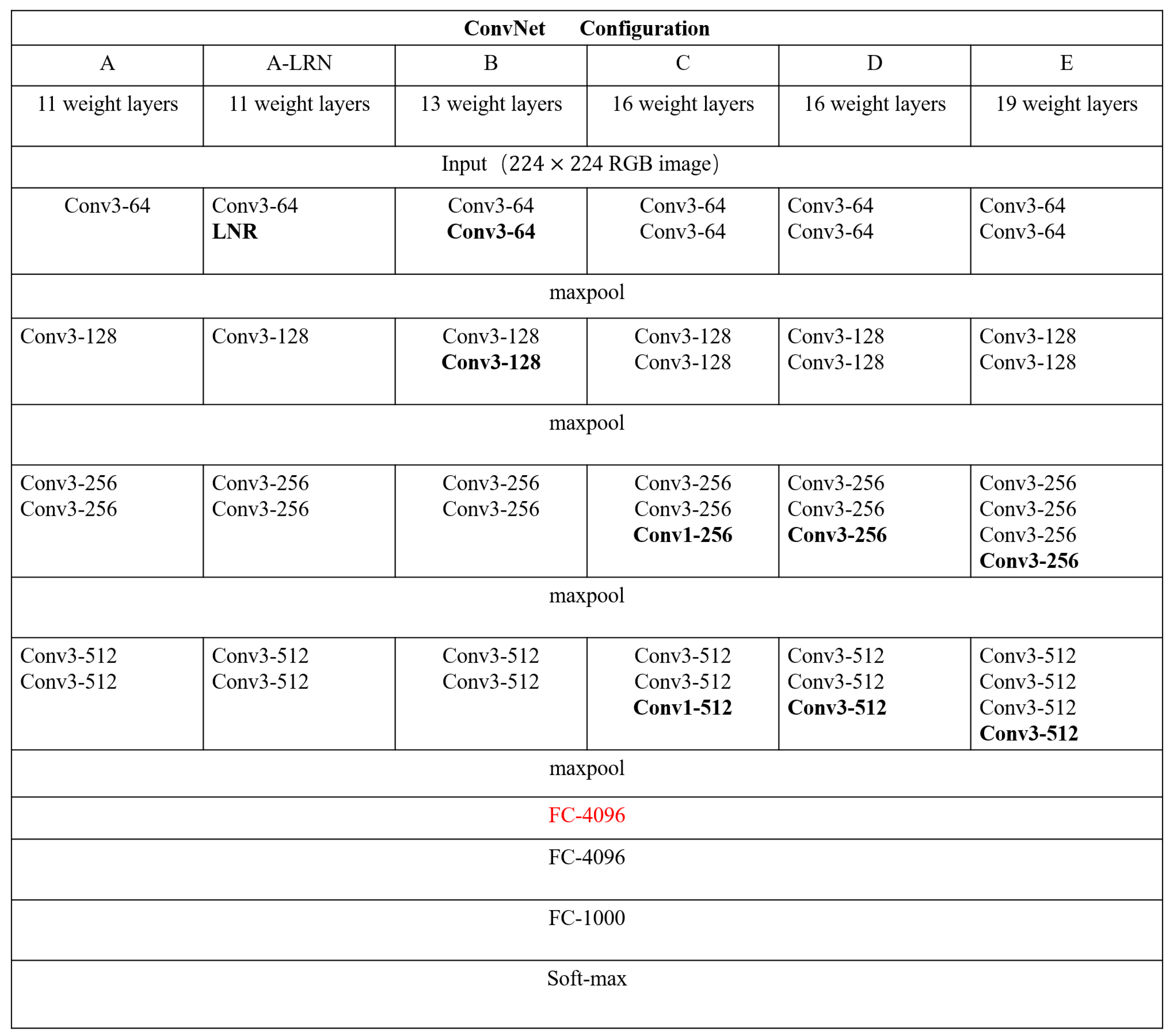
20] and VGG [21], to extract the feature. For the ResNet model, the ’pool5’ layer was utilized as the output layer to extract a 2048-dimensional vector for each image (as shown in Figure 3). For the VGG model, the ’fc6’ layer was utilized as the output layer to extract a 4096-dimensional vector for each image (As shown in Figure 4). Spatial pyramid matching is utilized, where the image is split into two layers, each of which has 1 and 5 segments, respectively (As shown in Figure 1). An image is represented as the concatenation of each segment with length 12,288-dimensional vector and 24,576-dimensional vector, respectively. The final feature of each image is 2 -normalized for better performance [19]. To eliminate randomness, we randomly (repeatable) split the dataset into the train set and test set for 10 times, respectively. Average accuracy was recorded.
The proposed SPM-CRC and WSPM-CRC algorithms are compared with other classification algorithms, including nearest-neighbor (NN) classification, LIBLINEAR [22], SOFTMAX, CRC [12], hybrid-KCRC [14], and SLRC-L2 [23].

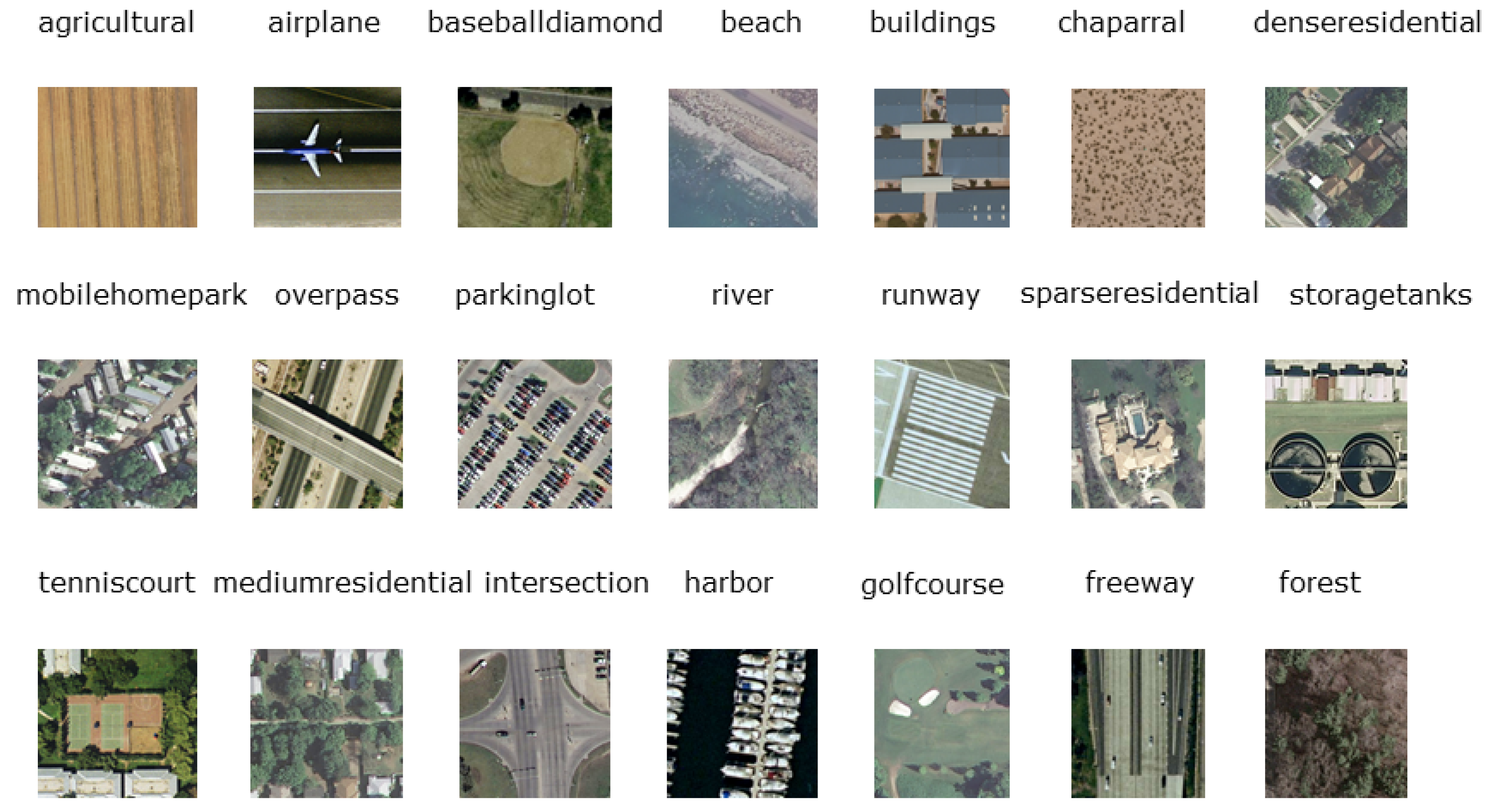
3.2. Experiment on UC Merced Land-Use Dataset

The UC Merced Land Use Dataset [17] consists of 2100 land-use images in total, collected from aerial orthoimages with a pixel resolution of one foot. The original images were downloaded from the United States Geological Survey National Map of 20 U.S. regions. The pixel resolution of this public-domain imagery was 1 foot. Each image measured 256 × 256 pixels. These images were manually selected into 21 classes: agricultural, airplane, baseball diamond, beach, buildings, chaparral, dense residential, forest, freeway, golf course, harbor, intersection, medium-density residential, mobile-home park, overpass, parking lot, river, runway, sparse residential, storage tanks, and tennis courts. In Figure 5, we list several samples from this dataset.

3.3. Parameter Tuning on UC Merced Land-Use Dataset

For the UC Merced Land Use Dataset, we randomly chose 20 images as the training samples and testing samples from each category, respectively. Only one parameter in the objection function of the SPM-CRC and WSPM-CRC algorithms needed to be specified. η is an important parameter in the SPM-CRC and WSPM-CRC algorithms, which is used to adjust the tradeoff between reconstruction error and collaborative representation. Additionally, η is tuned to achieve the best accuracy. For the feature extracted from both pretrained models, the optimal parameter η is 2 3 , 2 4 for SPM-CRC and WSPM-CRC, respectively.

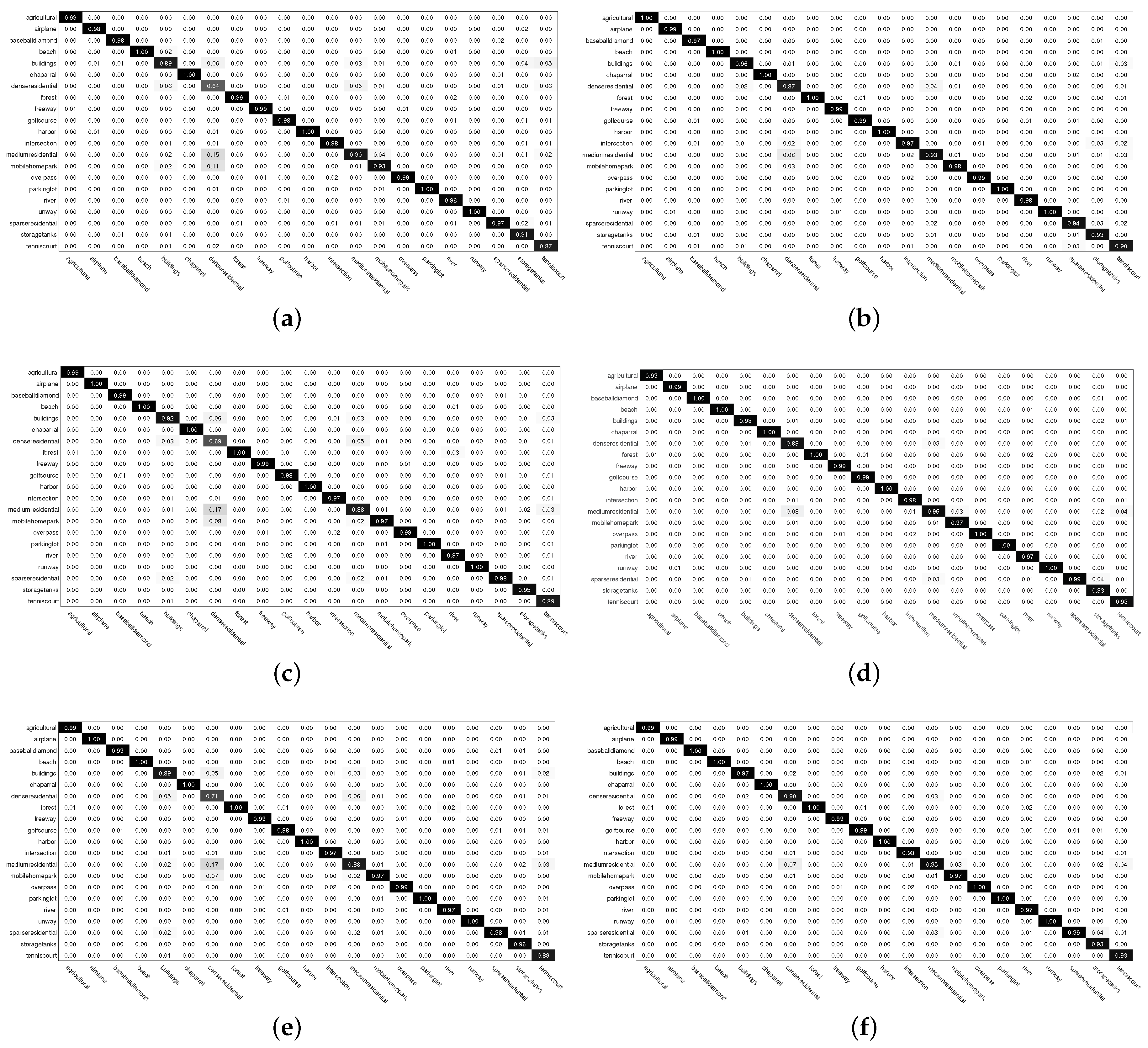
3.3.1. Confusion Matrix on UC Merced Land-Use Dataset

To further illustrate the superior performance of our proposed WPM-CRC method, we evaluated the classification rate per class of our method on the UC-Merced dataset using a confusion matrix. In this subsection, we randomly chose 80 images per class as training samples, and 20 images per class as testing samples. To eliminate randomness, we also randomly (repeatable) split the dataset into a train set and test set for 10 times, respectively. The confusion matrices are shown in Figure 6. From Figure 6, we can draw the following conclusions: (1) the ResNet model achieved better performance than the VGG model in most categories; (2) CRC with an SPM scheme achieved better performance than that without an SPM scheme; (3) compared with the SPM-CRC method, the WSPM-CRC method achieved better performance on the dense residential category.

3.3.2. Comparison with Several Classical Classifier Methods on UC Merced Land-Use Dataset

In this subsection, 20 and 20 samples per class were used for training and testing, respectively. Table 1 illustrates the effectiveness of SPM-CRC and WSPM-CRC for classifying images. For the ResNet model, when η is 2 4 , WSPM-CRC algorithm achieves the highest accuracy of 94.43 % . This is 1.64 % higher than the CRC method, and 0.12 % higher than the SPM-CRC method. For the VGG model, the WSPM-CRC algorithm exceeds the CRC method by 1.24 % , and the SPM-CRC method by 0.24 % .
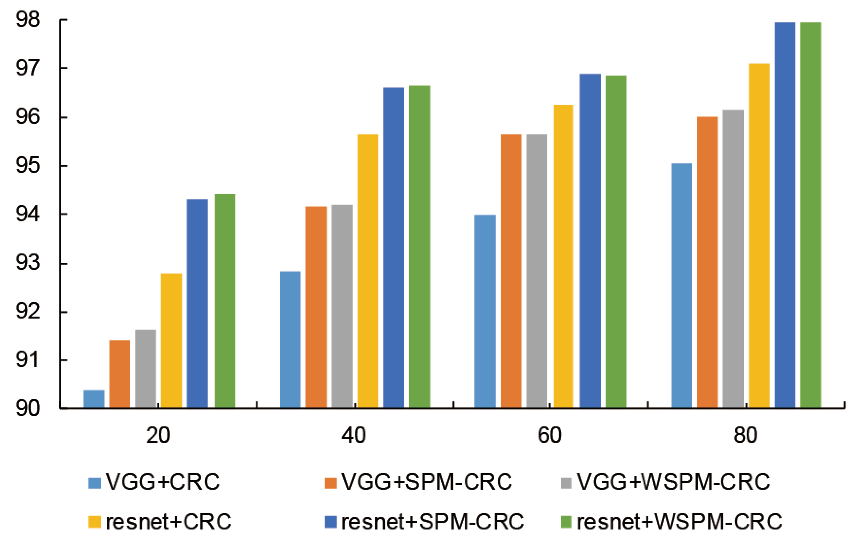
We increased the number of training samples in each category to evaluate the performance of our proposed WSPM-CRC method. Figure 7 shows the classification rate on the UC-Merced dataset with 20, 40, 60, and 80 training samples in each category. From Figure 7, we can conclude that our proposed WSPM-CRC method achieves superior performance to the CRC and SPM-CRC methods.

3.3.3. Comparison with State-of-the-Art Approaches

For comparison, we referred to previous work in the literature [24,25] and randomly selected 80 % of images of each class as the training set, and the remaining 20 % as the test set. Several baseline methods (e.g., liblinear and CRC) and state-of-the-art remote-sensing image-classification methods were used as the benchmark.
Table 2 shows the overall classification-rate accuracy of various remote-sensing image-classification methods. First, we compared the SPM-CRC and WSPM-CRC methods with liblinear and CRC. By comparing SPM-CRC and WSPM-CRC with the two baseline methods above, we found that the performance of SPM-CRC and WSPM-CRC was better than the two baseline methods. It is worth noting that the proposed WSPM-CRC is an improvement on the CRC method. Second, we compared SPM-CRC and WSPM-CRC with state-of-the-art remote-sensing image-classification results. Obviously, SPM-CRC and WSPM-CRC achieved the best performance. It should be noted that the feature utilized by CNN-W + VLAD with SVM, CNN-R + VLAD with SVM, and CaffeNet + VLAD is more effective than the feature extracted directly from the CNN (e.g., CaffeNet method, with 93.42 % , versus CaffeNet + VLAD method, with 95.39 % ).

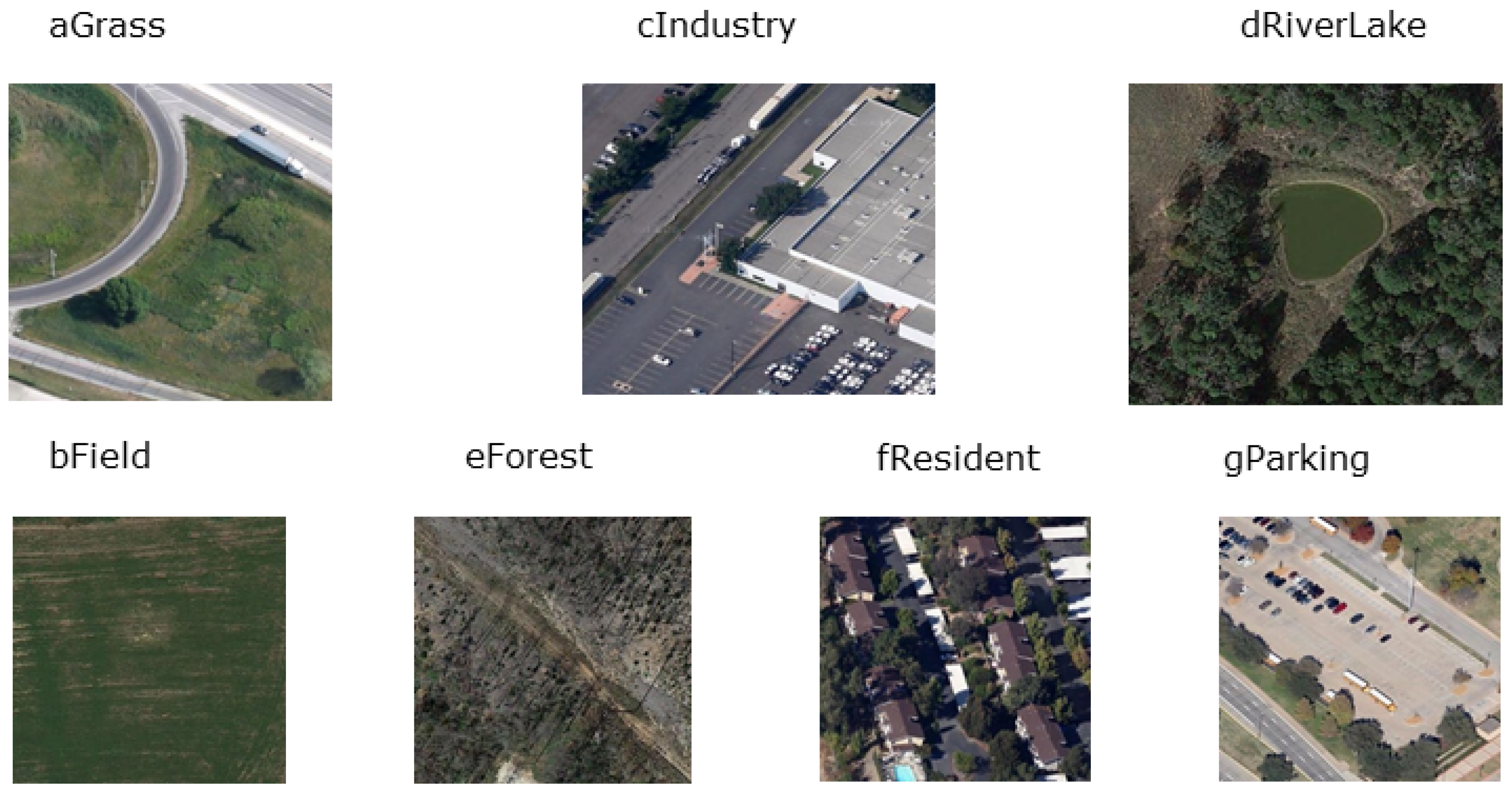
3.4. Experiment on RSSCN7 Dataset

RSSCN7 dataset consists of a total of 2100 land-use images collected from Google Earth. These images were manually selected into 7 classes: grassland, forest, farmland, industry, parking lot, residential, and river and lake region, where each class contains 400 images. Figure 8 shows several sample images from the dataset.
First, for comparison, we randomly selected 100 images from each class as the training set, and 100 more images as the testing set. Optimal parameter η is 2 3 , 2 4 for ResNet + SPM-CRC, and ResNet + WSPM-CRC, respectively. Optimal parameter η is 2 3 , 2 5 for VGG+SPM-CRC, and VGG + WSPM-CRC, respectively. Recognition accuracy is shown in Table 3. The best performance is marked with the bold. From Table 3, we can see that the SPM-CRC and WSPM-CRC methods outperformed other conventional methods. The WSPM-KCRC algorithm achieved the highest accuracy with 92.93 % .
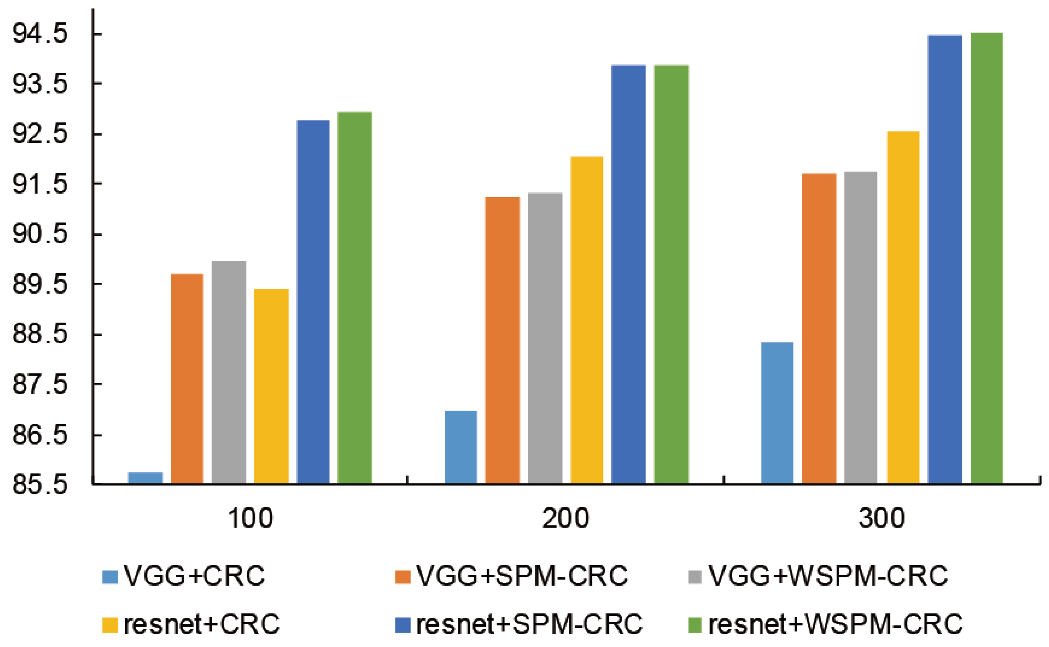
Second, we increased the number of training samples in each category to evaluate the performance of the SPM-CRC and WSPM-CRC methods. Figure 9 shows the classification rate on the RSSCN7 dataset with 100, 200, and 300 training samples in each category. From Figure 9, we found that both the SPM-CRC and WSPM-CRC method achieved superior performance to the baseline methods.

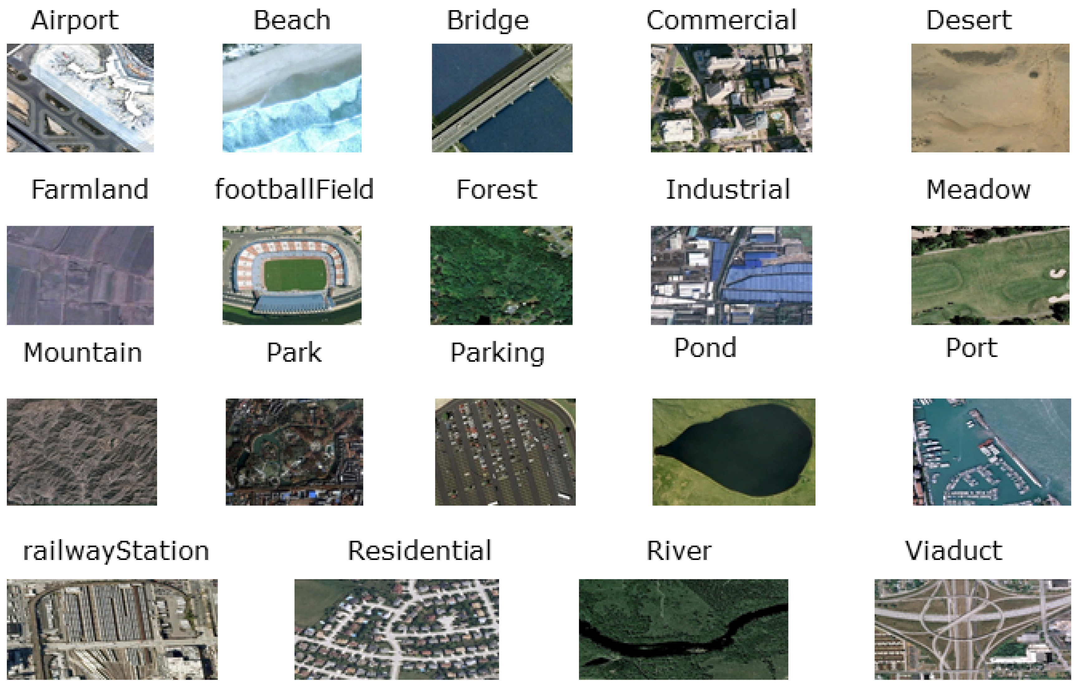
3.5. Experiment on the WHU-RS19 Dataset

WHU-RS19 dataset consists of 1005 aerial images in total, collected from Google Earth imagery. These images were manually selected into 19 classes. Figure 10 shows several sample images from the dataset.
For comparison, we randomly selected 20 images from each class as the training set, and 20 more images as the testing set. Optimal parameter η is 2 5 , 2 7 for ResNet + SPM-CRC, and ResNet + WSPM-CRC, respectively. Optimal parameter η is 2 3 , 2 4 for VGG + SPM-CRC, and VGG + WSPM-CRC, respectively. Recognition accuracy is shown in Table 4. The best performance is marked with the bold. From Table 4, we can see that the SPM-CRC and WSPM-CRC methods outperformed other conventional methods.

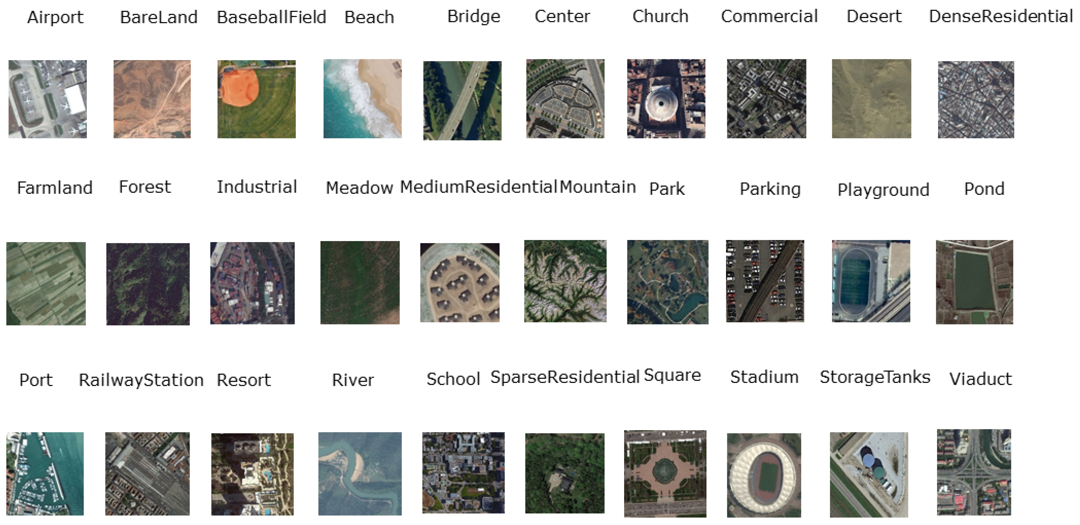
3.6. Experiment on the AID Dataset

The AID dataset is a new large-scale aerial-image dataset composed of 30 aerial-scene types: airport, bare land, baseball field, beach, bridge, center, church, commercial, dense residential, desert, farmland, forest, industrial, meadow, medium residential, mountain, park, parking, playground, pond, port, railway station, resort, river, school, sparse residential, square, stadium, storage tanks and viaduct and collected from Google Earth imagery. In addition, the AID dataset consists of a total of 10,000 images. In Figure 11, we show several images of this dataset.
For comparison, we randomly selected 20 images from each class as the training set and 20 more images as the testing set. OPptimal parameter η is 2 3 , 2 4 for ResNet + SPM-CRC, and ResNet + WSPM-CRC, respectively. Optimal parameter η is 2 2 , 2 4 for VGG + SPM-CRC, and VGG + WSPM-CRC, respectively. Recognition accuracy is shown in Table 5. The best performance is marked with the bold. From Table 5, we can see that the WSPM-CRC algorithm outperformed other conventional methods. The WSPM-CRC algorithm achieved the highest accuracy.

4. Discussion

  • For RS image classification, the weights to evaluate the representation of different subregions are fixed. In this paper, we proposed a spatial pyramid matching collaborative representation based classification method combined with CRC and the spatial pyramid matching approach to represent the image, which can decrease reconstruction error and improve classification rate. We compared our methods with several state-of-the-art methods for RS image classification, as shown in Table 6. The best performance is marked with the bold. Our proposed methods can effectively improve classification performance of remote-sensing images.
  • Because weights of different subregions in representing remote-sensing images are different, we learned the weights of different subregions to further improve the performance of the WSPM-CRC method. The classification rate on two pretrained CNN models with the WSPM-CRC method was higher than that with SPM-CRC.
  • We took UC-Merced dataset as an example and evaluated the performance of our proposed WSPM-CRC method per class with a confusion matrix. From the confusion matrix, we could see that the WSPM-CRC method is better than the other methods in most categories.

5. Conclusions

In this paper, we introduced a spatial pyramid matching scheme into the collaborative representation based classification method. The SPM-CRC approach considers spatial information in representing the image to improve performance in classifying remote-sensing images. We also learned the weights or contributions of each subregion in the SPM model. Thus, the WSPM-CRC method was applied to the spatial pyramid matching model to further improve image classification performance. Extensive experiments on four benchmark remote-sensing image datasets demonstrated the superiority of our proposed weighted spatial pyramid matching collaborative representation based classification algorithm.

Author Contributions

B.-D.L., W.-Y.X., J.M., S.S., and Y.L. conceived and designed the experiments; B.-D.L. and W.-Y.X. performed the experiments; Y.W. analyzed the data; W.X. and B.-D.L. wrote the paper; All authors read and approved the final manuscript.

Funding

This research was funded by the National Natural Science Foundation of China (Grant No. 61402535, No. 61271407), the Natural Science Foundation for Youths of Shandong Province, China (Grant No. ZR2014FQ001), the Natural Science Foundation of Shandong Province, China (Grant No. ZR2017MF069, ZR2018MF017), the Qingdao Science and Technology Project (No. 17-1-1-8-jch), the Fundamental Research Funds for the Central Universities, China University of Petroleum (East China) (Grant No. 16CX02060A, 17CX02027A), the Open Research Fund from Shandong Provincial Key Laboratory of Computer Network (No. SDKLCN-2018-01), and the Innovation Project for Graduate Students of China University of Petroleum (East China) (No. YCX2018063).

Conflicts of Interest

The authors declare no conflict of interest.

Abbreviations

The following abbreviations are used in this manuscript:
CRCCollaborative-Representation-Based Classification
CS-CRCClass-Specific Collaborative-Representation-Based Classification
RSRemote sensing
BoVWBag-of-visual-words
CNNsConvolutional Neural Networks
NNNearest Neighbor
SLRCSuperposed Linear Representation Classifier
SPMSpatial Pyramid Matching
WSPMWeighted Spatial Pyramid Matching

References

  1. Liu, W.; Ma, X.; Zhou, Y.; Tao, D.; Cheng, J. p-Laplacian regularization for scene recognition. IEEE Trans. Cybern. 2018. [Google Scholar] [CrossRef] [PubMed]
  2. Ma, X.; Liu, W.; Li, S.; Tao, D.; Zhou, Y. Hypergraph p-Laplacian Regularization for Remotely Sensed Image Recognition. IEEE Trans. Geosci. Remote Sens. 2018. [Google Scholar] [CrossRef]
  3. Csurka, G.; Dance, C.; Fan, L.; Willamowski, J.; Bray, C. Visual categorization with bags of keypoints. In Proceedings of the 8th European Conference on Computer Vision (ECCV 2004), Prague, Czech Republic, 11–14 May 2004; Volume 1, pp. 1–2. [Google Scholar]
  4. Olshausen, B.A.; Field, D.J. Sparse coding with an overcomplete basis set: A strategy employed by v1? Vis. Res. 1997, 37, 3311–3325. [Google Scholar] [CrossRef]
  5. Hinton, G.E.; Salakhutdinov, R.R. Reducing the dimensionality of data with neural networks. Science 2006, 313, 504–507. [Google Scholar] [CrossRef] [PubMed]
  6. Lazebnik, S.; Schmid, C.; Ponce, J. Beyond bags of features: Spatial pyramid matching for recognizing natural scene categories. In Proceedings of the IEEE Conference on Computer Vision and Pattern Recognition (CVPR 2006), New York, NY, USA, 17–22 June 2006; Volume 2, pp. 2169–2178. [Google Scholar]
  7. Morioka, N.; Satoh, S.I. Building compact local pairwise codebook with joint feature space clustering. In Proceedings of the 11th European Conference on Computer Vision (ECCV 2010), Heraklion, Crete, Greece, 5–11 September 2010; pp. 692–705. [Google Scholar]
  8. Morioka, N.; Satoh, S.I. Learning directional local pairwise bases with sparse coding. In Proceedings of the British Machine Vision Conference (BMVC 2010), Aberystwyth, UK, 31 August–3 September 2010; pp. 1–11. [Google Scholar]
  9. Nakayama, H.; Harada, T.; Kuniyoshi, Y. Global gaussian approach for scene categorization using information geometry. In Proceedings of the IEEE Conference on Computer Vision and Pattern Recognition (CVPR 2010), San Francisco, CA, USA, 13–18 June 2010; pp. 2336–2343. [Google Scholar]
  10. Harada, T.; Nakayama, H.; Kuniyoshi, Y. Improving local descriptors by embedding global and local spatial information. In Proceedings of the 11th European Conference on Computer Vision (ECCV 2010), Heraklion, Crete, Greece, 5–11 September 2010; pp. 736–749. [Google Scholar]
  11. Yang, J.; Yu, K.; Huang, T. Efficient highly over-complete sparse coding using a mixture model. In Proceedings of the 11th European Conference on Computer Vision (ECCV 2010), Heraklion, Crete, Greece, 5–11 September 2010; pp. 113–126. [Google Scholar]
  12. Zhang, L.; Yang, M.; Feng, X. Sparse representation or collaborative representation: Which helps face recognition? In Proceedings of the 2011 International Conference on Computer Vision (ICCV 2011), Barcelona, Spain, 6–13 November 2011; pp. 471–478. [Google Scholar]
  13. Li, J.; Zhang, H.; Zhang, L.; Huang, X.; Zhang, L. Joint Collaborative Representation with Multitask Learning for Hyperspectral Image Classification. IEEE Trans. Geosci. Remote Sens. 2014, 52, 5923–5936. [Google Scholar] [CrossRef]
  14. Liu, B.D.; Xie, W.Y.; Meng, J.; Li, Y.; Wang, Y.J. Hybrid collaborative representation for remote-sensing image scene classification. Remote Sens. 2018, 10, 1934. [Google Scholar] [CrossRef]
  15. Zorzi, M.; Chiuso, A. Sparse plus low rank network identification: A nonparametric approach. Automatica 2017, 76, 355–366. [Google Scholar] [CrossRef] [Green Version]
  16. Zou, Q.; Ni, L.; Zhang, T.; Wang, Q. Deep Learning Based Feature Selection for Remote Sensing Scene Classification. IEEE Geosci. Remote Sens. Lett. 2015, 12, 2321–2325. [Google Scholar] [CrossRef]
  17. Yang, Y.; Newsam, S. Bag-of-visual-words and spatial extensions for land-use classification. In Proceedings of the 18th SIGSPATIAL International Conference on Advances in Geographic Information Systems (GIS 2010), New York, NY, USA, 2–5 November 2010; pp. 270–279. [Google Scholar]
  18. Sheng, G.; Yang, W.; Xu, T.; Sun, H. High-resolution satellite scene classification using a sparse coding based multiple feature combination. Int. J. Remote Sens. 2012, 33, 2395–2412. [Google Scholar] [CrossRef]
  19. Xia, G.S.; Hu, J.; Hu, F.; Shi, B.; Bai, X.; Zhong, Y.; Lu, X. AID: A benchmark data set for performance evaluation of aerial scene classification. IEEE Trans. Geosci. Remote Sens. 2017, 55, 3965–3981. [Google Scholar] [CrossRef]
  20. He, K.; Zhang, X.; Ren, S.; Sun, J. Deep residual learning for image recognition. In Proceedings of the IEEE Conference on Computer Vision and Pattern Recognition (CVPR 2016), Las Vegas, NV, USA, 27–30 June 2016; pp. 770–778. [Google Scholar]
  21. Simonyan, K.; Zisserman, A. Very deep convolutional networks for large-scale image recognition. arXiv, 2014; arXiv:1409.1556. [Google Scholar]
  22. Fan, R.E.; Chang, K.W.; Hsieh, C.J.; Wang, X.R.; Lin, C.J. LIBLINEAR: A library for large linear classification. J. Mach. Learn. Res. 2008, 9, 1871–1874. [Google Scholar] [CrossRef]
  23. Deng, W.; Hu, J.; Guo, J. Face recognition via collaborative representation: Its discriminant nature and superposed representation. IEEE Trans. Pattern Anal. Mach. Intell. 2018, 40, 2513–2521. [Google Scholar] [CrossRef] [PubMed]
  24. Yu, Y.; Gong, Z.; Wang, C.; Zhong, P. An Unsupervised Convolutional Feature Fusion Network for Deep Representation of Remote Sensing Images. IEEE Geosci. Remote Sens. Lett. 2018, 15, 23–27. [Google Scholar] [CrossRef]
  25. Lu, X.; Zheng, X.; Yuan, Y. Remote sensing scene classification by unsupervised representation learning. IEEE Trans. Geosci. Remote Sens. 2017, 55, 5148–5157. [Google Scholar] [CrossRef]
  26. Văduva, C.; Gavăt, I.; Datcu, M. Latent Dirichlet allocation for spatial analysis of satellite images. IEEE Trans. Geosci. Remote Sens. 2013, 51, 2770–2786. [Google Scholar] [CrossRef]
  27. Cheriyadat, A.M. Unsupervised feature learning for aerial scene classification. IEEE Trans. Geosci. Remote Sens. 2014, 52, 439–451. [Google Scholar] [CrossRef]
  28. Zhang, F.; Du, B.; Zhang, L. Saliency-guided unsupervised feature learning for scene classification. IEEE Trans. Geosci. Remote Sens. 2015, 53, 2175–2184. [Google Scholar] [CrossRef]
  29. Penatti, O.A.; Nogueira, K.; Dos Santos, J.A. Do deep features generalize from everyday objects to remote sensing and aerial scenes domains? In Proceedings of the IEEE International Conference on Computer Vision and Pattern Recognition (CVPR 2015), Boston, MA, USA, 8–10 June 2015; pp. 44–51. [Google Scholar]
  30. Hu, F.; Xia, G.S.; Hu, J.; Zhang, L. Transferring deep convolutional neural networks for the scene classification of high-resolution remote sensing imagery. Remote Sens. 2015, 7, 14680–14707. [Google Scholar] [CrossRef]
  31. Lin, D.; Fu, K.; Wang, Y.; Xu, G.; Sun, X. MARTA GANs: Unsupervised representation learning for remote sensing image classification. IEEE Geosci. Remote Sens. Lett. 2017, 14, 2092–2096. [Google Scholar] [CrossRef]
  32. Li, P.; Ren, P.; Zhang, X.; Wang, Q.; Zhu, X.; Wang, L. Region-Wise Deep Feature Representation for Remote Sensing Images. Remote Sens. 2018, 10, 871. [Google Scholar] [CrossRef]
Figure 1. Scheme of our proposed weighted spatial pyramid matching scheme. (Left) conventional spatial pyramid matching (SPM) model whose weights to evaluate the representation of different subregions are fixed; (Right) weighted spatial pyramid matching.
Remotesensing 11 00518 g001
Figure 2. An example of a three-level pyramid model. Image is represented in three levels. For each level, the image is split into 1, 4, and 16 segments, respectively. For level 0, the representation of the image is statistical information and does not include spatial information. As the number of segments increases, more spatial information is obtained. For each subimage, the feature is independently extracted. All features are concatenated to form a feature vector to describe the image.
Remotesensing 11 00518 g002
Figure 3. ResNet structure. In this paper, we used 152-layer architecture. For each image, we adopted the ’pool5’ layer as the output layer that forms a 2048 dimensional vector.
Remotesensing 11 00518 g003
Figure 4. VGG structure. In this paper, we used 19 weight layers (VGG-19). For each image, we used the first FC-4096 as the output layer. Therefore, the dimension was 4096.
Remotesensing 11 00518 g004
Figure 5. Example images of the UC-Merced dataset. The dataset has 21 remote-sensing categories in total.
Remotesensing 11 00518 g005
Figure 6. Confusion matrices on the UC-Merced dataset. (a) VGG + CRC; (b) resnet + CRC; (c) VGG + SPM-CRC; (d) resnet + SPM-CRC; (e) VGG + WSPM-CRC; (f) resnet + WSPM-CRC.
Remotesensing 11 00518 g006
Figure 7. Classification rate on the UC-Merced dataset with a different number of training samples in each category.
Remotesensing 11 00518 g007
Figure 8. Example images of the RSSCN7 dataset. RSSCN7 has a total of seven remote-sensing categories.
Remotesensing 11 00518 g008
Figure 9. Classification rate on the RSSCN7 dataset with a different number of training samples in each category.
Remotesensing 11 00518 g009
Figure 10. Example images of WHU-RS19 dataset. The dataset has 19 remote-sensing categories in total.
Remotesensing 11 00518 g010
Figure 11. Example images of AID dataset. The dataset has 30 remote-sensing categories in total.
Remotesensing 11 00518 g011
Table 1. Comparison with several classical classification methods on the UC Merced Land-Use Dataset (%).
Methods\DatasetsUC-Merced
VGG19 + NN81.88
VGG19 + LIBLINEAR89.57
VGG19 + SOFTMAX88.00
VGG19 + SLRC-L289.79
VGG19 + CRC90.40
VGG19 + CS-CRC89.10
resnet + CRC92.79
VGG19 + Hybrid-KCRC (linear) [14]90.67
VGG19 + Hybrid-KCRC (POLY) [14]91.43
VGG19 + Hybrid-KCRC (RBF) [14]91.43
VGG19 + Hybrid-KCRC (Hellinger) [14]90.90
VGG19 + SPM-KCRC91.4
VGG19 + WSPM-KCRC91.64
resnet + SPM-CRC94.31
resnet + WSPM-CRC94.43
Table 2. Experiment on UC-Merced dataset (%).
MethodsYearAccuracy
SPMK [6]2006 74 %
LDA-SVM [26]2013 80.33 %
SIFT + SC [27]2013 81.67 %
Saliency + SC [28]2014 82.72 %
CaffeNet [29] (without fine-tuning)2015 93.42 %
CaffeNet [30] + VLAD2015 95.39 %
DCGANs [31] (without augmentation)2017 85.36 %
MAGANs [31] (without augmentation)2017 87.69 %
WDM [25]2017 95.71 %
UCFFN [24]2018 87.83 %
CNN-W + VLAD with SVM [32]2018 95.61 %
CNN-R + VLAD with SVM [32]2018 95.85 %
VGG19 + liblinear 95.05 %
VGG19 + CRC 94.67 %
VGG19 + CS-CRC 95.26 %
resnet+CRC 96.9 %
VGG19 + Hybrid-KCRC (linear) [14]2018 96.17 %
VGG19 + Hybrid-KCRC (POLY) [14]2018 96.29 %
VGG19 + Hybrid-KCRC (RBF) [14]2018 96.26 %
VGG19 + Hybrid-KCRC (Hellinger) [14]2018 96.33 %
VGG19 + SPM-KCRC 96.02 %
VGG19 + WSPM-KCRC 96.14 %
resnet + SPM-CRC 97.95 %
resnet + WSPM-CRC 97.95 %
Table 3. Comparison with several classical classification methods on the RSSCN7 dataset (%).
Methods\DatasetsRSSCN7
VGG19 + NN76.44
VGG19 + LIBLINEAR84.84
VGG19 + SOFTMAX82.14
VGG19 + SLRC-L281.99
VGG19 + CRC85.77
VGG19 + CS-CRC84.23
resnet + CRC89.43
Hybrid-KCRC (linear)86.39
Hybrid-KCRC (POLY)87.34
Hybrid-KCRC (RBF)87.29
Hybrid-KCRC (Hellinger)86.71
VGG19 + SPM-CRC89.71
VGG19 + WSPM-CRC89.97
resnet + SPM-CRC92.79
resnet + WSPM-CRC92.93
Table 4. Comparison with several classical classification methods on the WHU-RS19 dataset (%).
Methods\DatasetsWHU-RS19
VGG19 + NN87.74
VGG19 + LIBLINEAR94.42
VGG19 + SOFTMAX93.29
VGG19 + SLRC-L294.18
VGG19 + CRC94.58
VGG19 + CS-CRC93.95
resnet + CRC97.11
Hybrid-KCRC (linear)94.76
Hybrid-KCRC (POLY)95.34
Hybrid-KCRC (RBF)95.34
Hybrid-KCRC (Hellinger)95.39
VGG19 + SPM-CRC96.68
VGG19 + WSPM-CRC96.76
resnet + SPM-CRC97.76
resnet + WSPM-CRC97.74
Table 5. Comparison with several classical classification methods on the AID dataset (%).
Methods\DatasetsAID
VGG19 + NN65.32
VGG19 + LIBLINEAR79.93
VGG19 + SOFTMAX76.13
VGG19 + SLRC-L279.27
VGG19 + CRC80.73
VGG19 + CS-CRC77.92
resnet + CRC85.28
Hybrid-KCRC (linear)81.07
Hybrid-KCRC (POLY)82.07
Hybrid-KCRC (RBF)82.05
Hybrid-KCRC (Hellinger)81.28
VGG19 + SPM-CRC84.57
VGG19 + WSPM-CRC84.63
resnet + SPM-CRC88.27
resnet + WSPM-CRC88.28
Table 6. Comparison with different CNN pretrained models (%).
Models\DatasetsUC-Merced (0.8)WHU-RS19 (0.6)RSSCN7 (0.5)AID (0.5)
CaffeNet + SVM [19]95.0296.2488.2589.53
VGG16 + SVM [19]95.2196.0587.1889.64
GoogleNet + SVM [19]94.3194.7185.8486.39
VGG19 + SVM [14]94.6795.4285.9990.35
VGG19 + CRC [14]95.0595.6386.9789.58
VGG19 + Hybrid-KCRC (linear) [14]96.1795.6888.1689.93
VGG19 + Hybrid-KCRC (POLY) [14]96.2996.4289.2191.75
VGG19 + Hybrid-KCRC (RBF) [14]96.2696.589.1791.82
VGG19 + Hybrid-KCRC (Hellinger) [14]96.3395.8288.4790.35
Resnet + SVM [14]96.9097.7491.592.97
Resnet + CRC [14]97.0098.0392.0692.85
Resnet + Hybrid-KCRC (linear) [14]97.2998.0592.8992.87
Resnet + Hybrid-KCRC (POLY) [14]97.4098.1693.1193.98
Resnet + Hybrid-KCRC (RBF) [14]97.4398.1393.0794.00
Resnet + Hybrid-KCRC (Hellinger) [14]97.3698.3792.8793.15
VGG19 + SPM-CRC96.0297.3791.2692.55
VGG19 + WSPM-CRC96.1497.3791.3192.57
Resnet + SPM-CRC97.9598.2693.8695.1
Resnet + WSPM-CRC97.9598.3293.995.11

