Rock Location and Quantitative Analysis of Regolith at the Chang’e 3 Landing Site Based on Local Similarity Constraint


1
College of Geo-Exploration Science and Technology, Jilin University, Changchun 130026, China
2
Ministry of Land and Resources Key Laboratory of Applied Geophysics, Jilin University, Changchun 130026, China
*
Author to whom correspondence should be addressed.
Remote Sens. 2019, 11(5), 530; https://0-doi-org.brum.beds.ac.uk/10.3390/rs11050530
Submission received: 24 January 2019
/
Revised: 1 March 2019
/
Accepted: 2 March 2019
/
Published: 5 March 2019
(This article belongs to the Special Issue Recent Progress in Ground Penetrating Radar Remote Sensing)
Abstract
:Structural analysis of lunar regolith not only provides important information about lunar geology but also provides a reference for future lunar sample return missions. The Lunar Penetrating Radar (LPR) onboard China’s Chang’E-3 (CE-3) provides a unique opportunity for mapping the subsurface structure and the near-surface stratigraphic structure of the regolith. The problem of rock positioning and regolith-basement interface highlighting is meaningful. In this paper, we propose an adaptive rock extraction method based on local similarity constraints to achieve the rock location and quantitative analysis for regolith. Firstly, a processing pipeline is designed to image the LPR CH-2 A and B data. Secondly, we adopt an f-x EMD (empirical mode decomposition)-based dip filter to extract low-wavenumber components in the two data. Then, we calculate the local similarity spectrum between the filtered CH-2 A and B. After a soft threshold function, we pick the local maximums in the spectrum as the location of each rock. Finally, according to the extracted result, on the one hand, the depth of regolith is obtained, and on the other hand, the distribution information of the rocks in regolith, which changes with the path and the depth, is also revealed.
1. Introduction
Chang’E-3 landed at 340.4875 °E, 44.1189 °N on the Moon on 14 December 2013 in a new region that has not been explored before in the largest basin—the Mare Imbrium [1]. The dual-frequency Lunar Penetrating Radar aboard the Yutu Rover provides a unique opportunity to map the subsurface structure to a depth of several hundreds of metres from the low-frequency channel (CH-1, 60 MHz) and the near-surface stratigraphic structure of the regolith from the high-frequency channel (CH-2A &CH-2B, 500 MHz). The LPR also provides an accurate detection result with high resolution from high-frequency observations [2].
LPR data processing and initial results were first presented by NAOC [3]. Initial analysis of the LPR observations, especially that from the CH-1, indicates that there are more than nine subsurface layers from the surface to a depth of ~360 m [1]. The onboard Lunar Penetrating Radar conducted a 114-m-long profile, which measured a thickness of ~5 m of the lunar regolith layer and detected three underlying basalt units at depths of 195, 215, and 345 m. The radar measurements suggest an underestimation of the global lunar regolith thickness by other methods and reveal a vast volume from the last volcanic eruption [4]. Fa et al., Lai et al. and Zhang et al. speculated the near surface structure by processing the raw CH-2B data [5,6,7]. Dong et al. and Zhang et al. calculated the parameters of the regolith [8,9].
The previous papers mainly studied the geological stratification and parameter inversion of regolith by using CH-2B data. The quantity and location of rocks in regolith have not been researched and CH-2A data have not been fully used. The quantity and location of rocks in regolith not only help to understand the evolution of regolith on the landing site but also provide a priori information for the further CE-5 plan of regolith collection. The rocks in lunar regolith are the break point, causing diffractions in LPR data. The kinematics characteristics of these diffractions are quite different from those of main reflections, which is expressed as a hyperbola in common offset sections [10,11]. The vertex position of the diffractions indicates the location of rocks. Therefore, to reach this goal, a method for extracting low-wavenumber components of diffractions and taking full advantages of both LPR CH-2A and CH-2B data is needed.
Huang et al. [12] uses empirical mode decomposition (EMD) to prepare stable input for the Hilbert transform. The aim of EMD is stabilizing a nonstationary signal and decomposing the nonstationary signal into fast and slow oscillation components, called intrinsic mode functions (IMFs). 1D EMD can be an adaptive band-pass filter, dividing the dataset into the IMFs with different frequency range. As the property of EMD, Bekara and van der Baan [13] propose f-x EMD to attenuate the random and coherent noise. Cai et al. [14] propose the guideline of t-f-x EMD denoising. Chen et al. [15] add an autoregressive (AR) model to f-x EMD to improve the applicable conditions and adopt f-x EMD as an effective tool for dip filter.
Local similarity is a typical local attribute and promising for quantifying the similarity of two datasets in a non-instantaneous and non-global manner [16]. Different from traditional attributes, it is calculated using every element of the LPR data and its adjoining elements within a definite scope, which has been utilized in many signal processing fields such as image contrast [17,18], time-frequency analysis [19], noise attenuation [20,21], deblending [22]. The basic criterion of image contrast in this method is the different similarity between signal and noise, i.e., the signal denotes a large value in the local similarity spectrum. In this way, noise and artifacts can be attenuated by using a threshold function.
In this paper, we propose an adaptive rock extraction method based on local similarity constrains to achieve the rock location and quantitative analysis for regolith. Firstly, a processing pipeline is designed to image the LPR CH-2 A and B data. Secondly, we adopt f-x EMD-based dip filter to extract low-wavenumber components in the two data. Then, we calculate the local similarity spectrum between the filtered CH-2 A and B. After a soft threshold function, we pick the local maximums in the spectrum as the location of each rock. Finally, according to the extracted result, on the one hand, the depth of regolith is obtained, and on the other hand, the distribution information of the rocks in regolith, which changes with the path and the depth, is also revealed.
2. Materials and Methods
2.1. LPR Data Processing
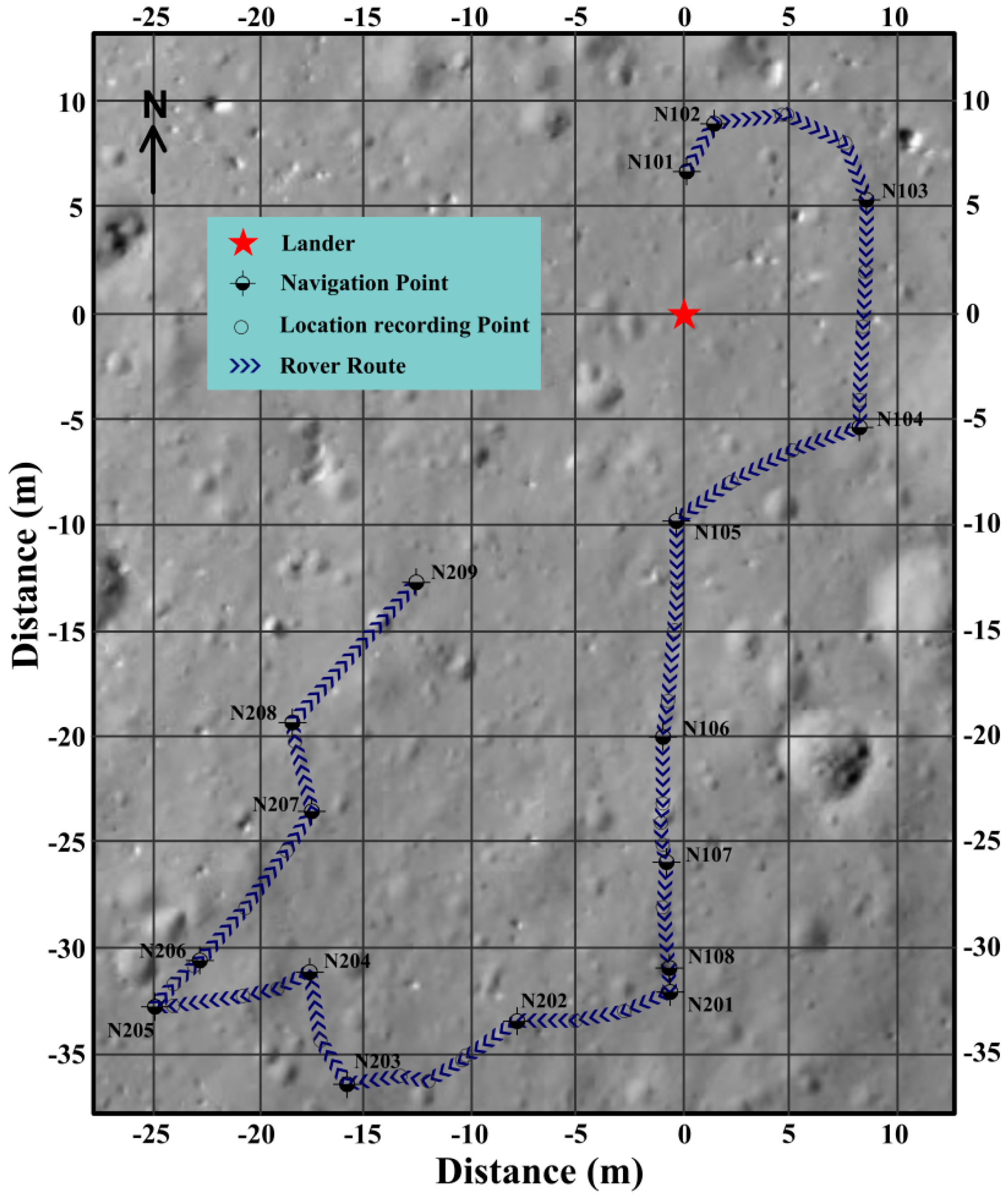
Yutu Rover released by CE-3 was the first soft landing on the Moon since the Soviet Union’s Luna 24 mission in 1976. To be specific, the Yutu rover explored the surface and subsurface of the landing site in the northern part of the Mare Imbrium using its four main instruments: the Panoramic Camera, Lunar Penetrating Radar (LPR), Visible–Near Infrared Spectrometer (VNIS), and Active Particle-Induced X-ray Spectrometer (APXS). Its track extends to 114.8 m (Figure 1) near a young crater. In this part, the data processing results of the LPR are reported.
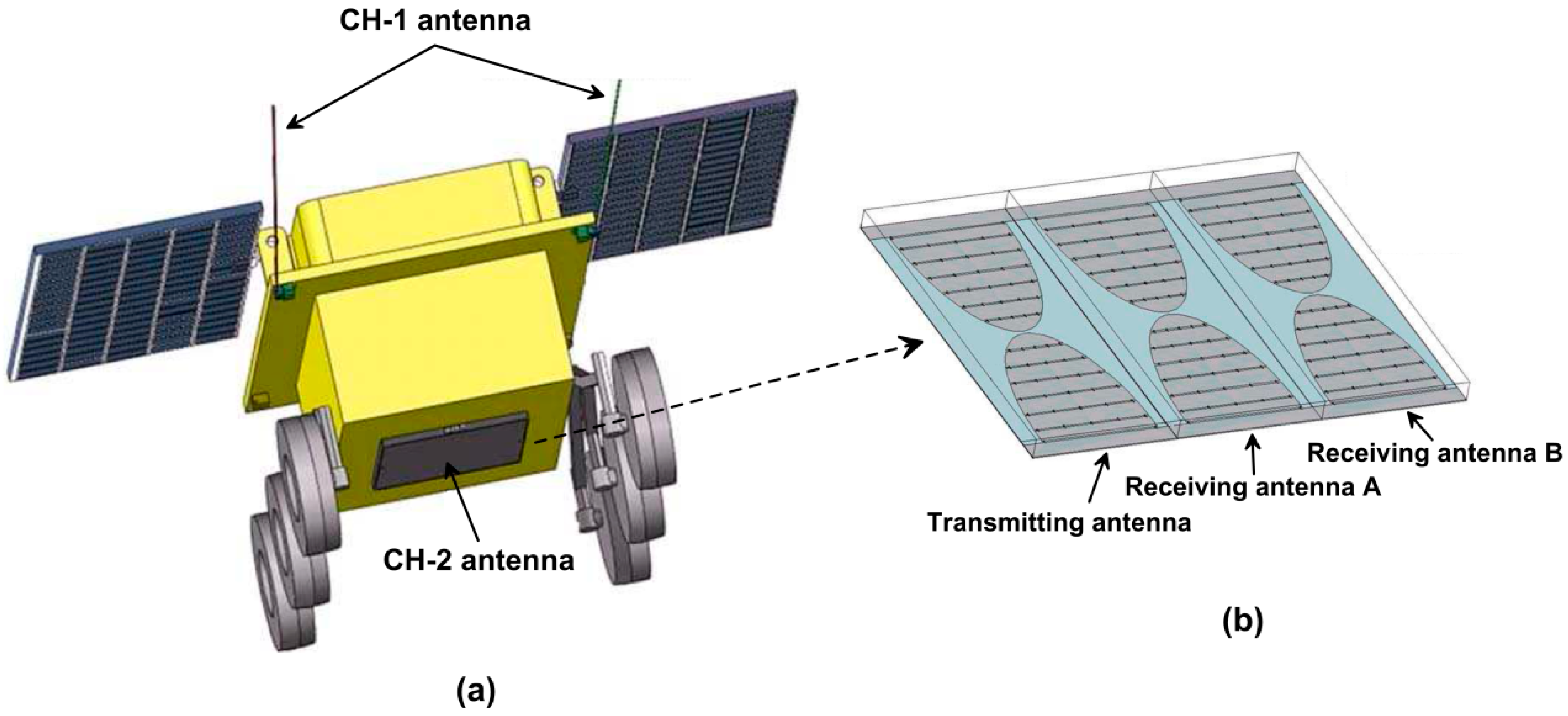
Aiming at the near-surface stratigraphic structure of the regolith, CH-2 antenna is selected. The CH-2 antenna is mounted at the bottom of lunar rover (Figure 2a), which is about 30 cm away from the ground. Figure 2b shows the structure of the CH2 antenna. As can be seen from the figure, the CH2 antenna has three antenna elements. The antenna elements are arranged side by side in a metal back cavity which is divided into three individual cavities. One antenna element is used to transmit EM waves and the other two are used to receive the EM waves. Each antenna element is 336 mm in length and 120 mm in width, and the space between the antenna elements is about 160 mm. The height of the back cavity of the antenna is reduced to 22 mm from a quarter of the center wavelength in order to ensure the lunar rover can maneuver over obstacles [2].
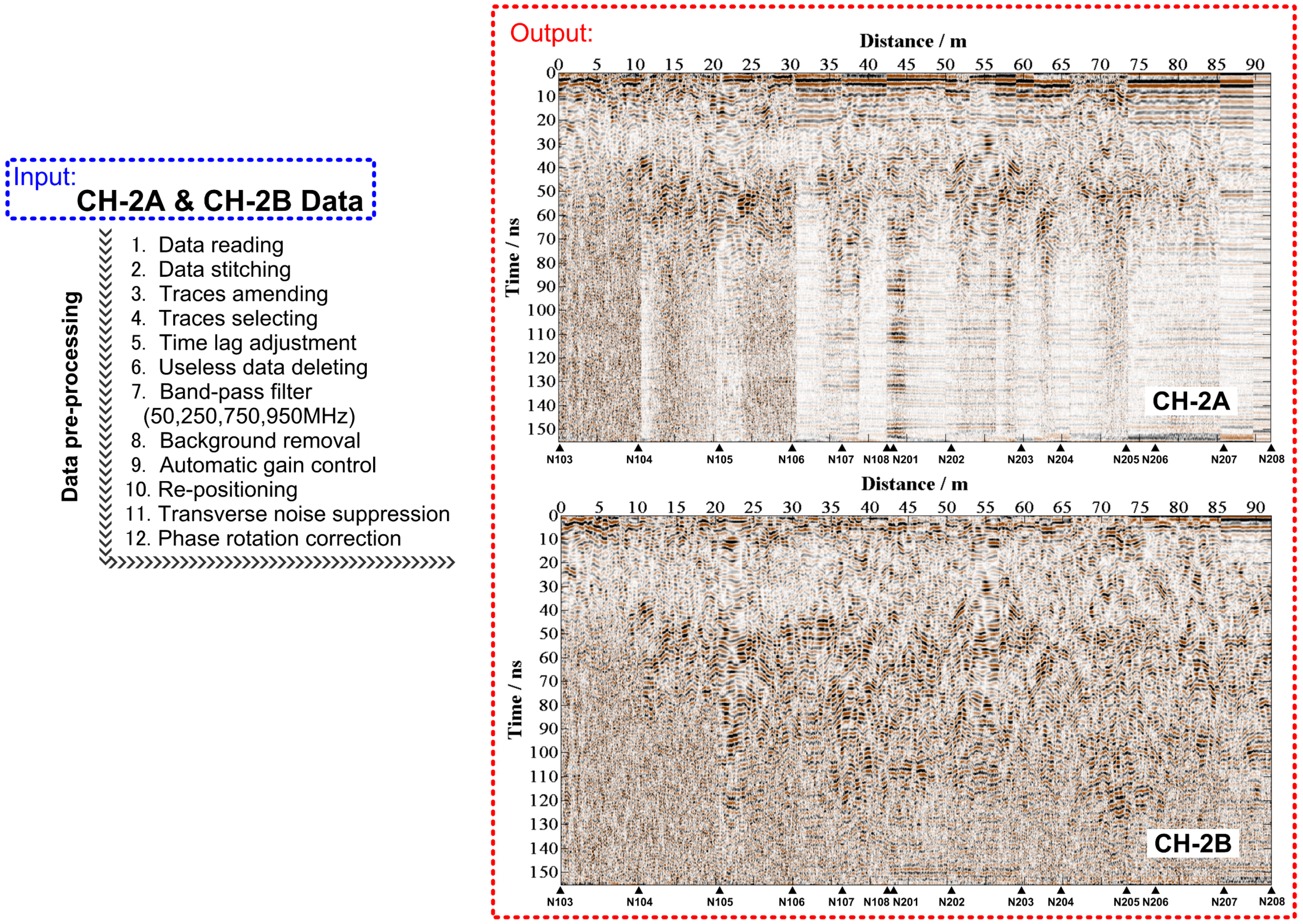
As the tight arrangement of the antennas, two sets of 500 MHz data (CH-2A & CH-2B) are achieved and their data quality should be similar. However, due to the complex acquisition environment and inappropriate instrument parameter settings, the CH-2A data has a lower SNR (signal-to-noise ratio) than the CH-2B data. Therefore, the former papers only focused on the CH-2B data. In order to make full use of CH-2A and CH-2B data, according to the acquisition parameters, the actual situation, and the data quality, the LPR data processing pipeline is designed (Figure 3). Note that the non-uniform patrol mode and uninterrupted collection of the rover cause the problem of uneven sampling. After data editing and processing, the high-resolution radar images with 497 samples, 4595 traces and 0.02 m spatial interval are accessible. The IDs for the data from Lunar Penetrating Radar are listed in Appendix A in the Supporting Materials.
The previous papers mainly studied on the geological stratification and parameter inversion. The quantity and location of rocks in regolith have not been researched. The quantity and location of rocks in regolith not only help to understand the evolution of regolith on the landing site but also provide a priori information for the further CE-5 plan of regolith collection. In the following method, we propose a rock extraction method based on local similarity constrains to achieve the rock location and quantitative analysis for regolith.
2.2. An f-x Domain EMD-Based Dip Filter
EMD can provide an empirical decomposition of a non-stationary signal. These decomposed sub-signals are separated based on oscillation frequency and called IMFs. A stable IMF has a constant instantaneous frequency and narrow-band waveform, satisfying two conditions [12]: (1) the number of extremes and zero crossings in the data series are either equal or differ by one, and (2) at any points, the mean value of the envelope defined by the local maxima and the local minima is zero.
In the 1D case, the signal is decomposed into several sub-signals with different frequency ranges, which can be written as
where is the input signal and is the decomposed IMFs. denotes the residual and N is the IMF number.
As the advantages of signal decomposition, Bekara and van der Baan [13] adopt EMD in f-x domain to suppress random noise and steep dip coherent noise. They consider the noise energy is dominant in the high wavenumber portion in the f-x domain. The high wavenumber portion presents the fast oscillation of each frequency slice. Based on the separation between the noise and signal, noise can be attenuated by simply removing IMF1 from noisy data. The detailed process is shown as follows:
- (1)
- Set the size of the time window.
- (2)
- Pick a time window and adopt 1D forward Fourier transform along the time direction.
- (3)
- Pick a frequency slice and separate it into real and imaginary parts.
- (4)
- Compute IMF1s for real and imaginary parts to obtain the filtered parts.
- (5)
- Compose the filtered frequency slice.
- (6)
- Repeat (4)–(5) for each frequency slice.
- (7)
- Adopt 1D reverse Fourier transform along the time direction.
- (8)
- Repeat (2)–(7) for each time window.
The two advantages of f-x EMD are convenience and stability. The f-x EMD is a data-driven f-k filter and does not require the predefined muting zone in the f-k domain, which is easily embedded into field data processing. Moreover, unlike convolutional operator-based denoising methods (such as f-x predictive filter), f-x EMD can deal with an irregular spatial sampling dataset [13,23]. For data acquisition of LPR, irregular spatial sampling is inevitable because of the complex terrain, finite time and expensive cost. Therefore, f-x EMD is a promising tool in LPR data processing.
It should also be noted that the choice of the removed IMFs can be more than one. The choice is determined by dispersion of high wavenumber components and noise level. When the target noise is located in high wavenumber components or the noise level is low, the number of removed IMFs can be small. Conversely, more IMFs should be removed.
Since the dip angle of the signal is related to wavenumber, f-x EMD can be used as a dip filter [15]. The different IMFs present different dip angle ranges, i.e., high dip components locate in the low IMFs and low dip components locate in the high IMFs. If we divide the IMF set into several subsets, the dataset is separated by the dip angle. Therefore, we define the dip filter using f-x EMD as follows:
where is the filtered frequency slice and is the ith separated IMF. is the ith dip subsets and m is the number of divided subsets. denotes the weighting factors.
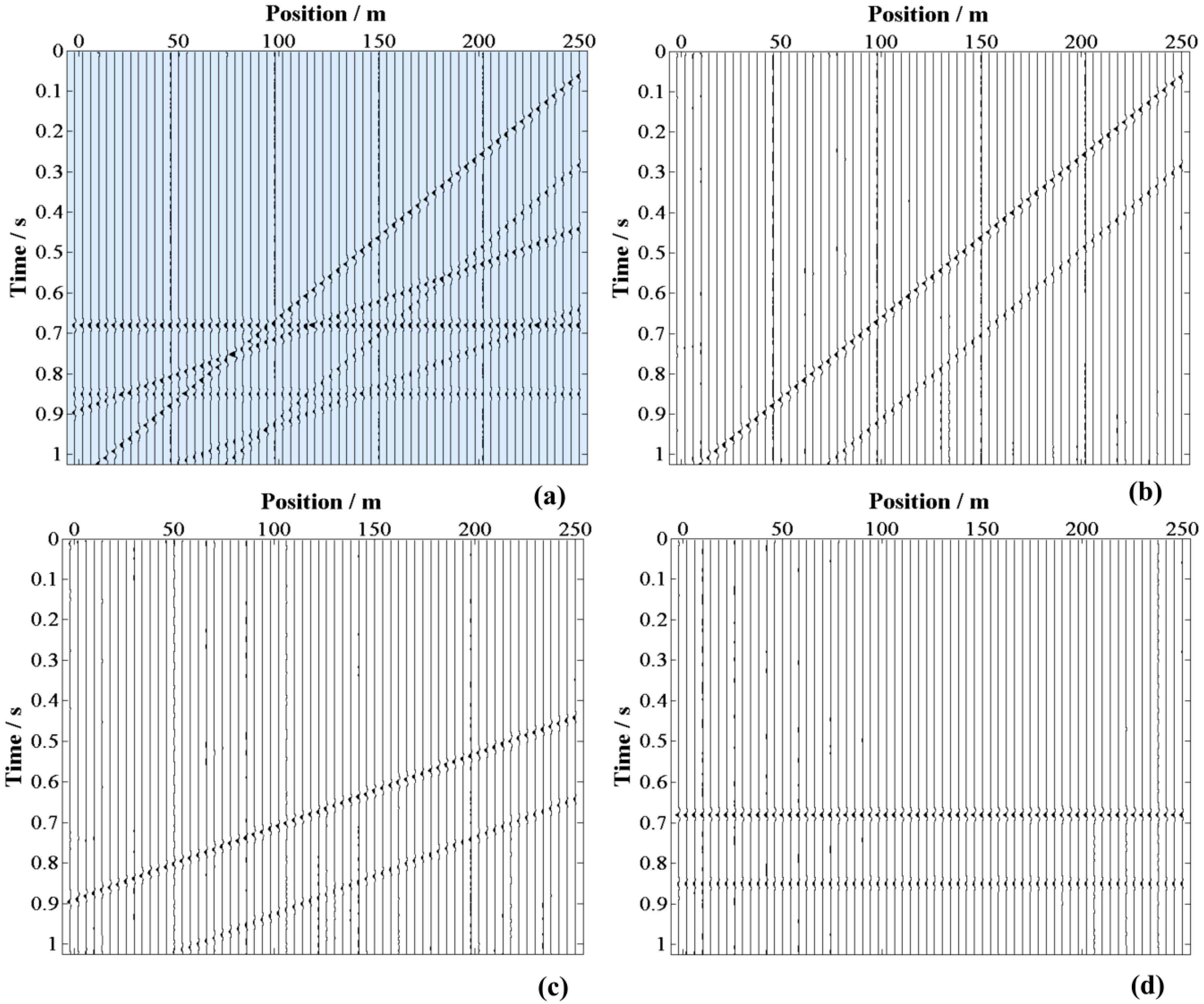
Figure 4 demonstrates the results of three types of dip filters (high-pass, mid-pass and low-pass) working on a plane wave model. In the synthetic data (Figure 4a), the dataset contains three dip sets. After the three dip filters, different dip events (Figure 4b–d) are well extracted. Table 1 shows the detailed parameters of the three filters. The LPR data are acquired in a constant-offset way, whose source can be considered as wave plane. The kinematics characteristics of the main reflection events are similar to that of the terrain. The rock in lunar regolith is the break point, causing diffractions in LPR data. The kinematics characteristics of these diffractions are hyperbola. In a word, the reflection events are low dip and smooth, whereas the diffraction events show a high dip. The diffraction point extraction can be transformed into a problem of steep dip decreasing. Therefore, we should select a simple low-pass dip filter, with , , , . The key parameter is the number of removed IMFs .
2.3. Rock Extraction Based on Local Similarity Constraint
For quantitative analysis, the problem of rock positioning is commonly picking the local maximums in the filtered data. However, as shown in Figure 2, the preprocessed LPR CH-2 A and B data are interfered with by noise. The strong coherence of noise leads to many noise-caused local maximums, which reduces the accuracy of rock extraction. To take full advantages of both LPR CH-2A and CH-2B data and reduce the effects of noise, we introduce local similarity (see Appendix B) in the process of rock positioning. The basic idea is the similarity difference between the signal and noise in two similar datasets. We consider the two noisy datasets (D) are a totalization of noise (N) and signal (S):
The noise is caused by ambient disturbance, instrument defect, etc., which has little relationship with underground structure, and the signal is just the opposite. In a word, if the observing system is the same, the signal will have larger similarity than the noise. We calculate the local similarity spectrum between the two data points to quantify the difference in similarity. We consider the local similarity (c) between two noisy datasets as
and Equation (6) can be easily modified as
We utilize a soft threshold function modifies to attenuate the noise interference. We obtain an approximate signal-dominated local similarity spectrum:
where is the threshold value and i, j is the sample coordinates in the time-space domain.
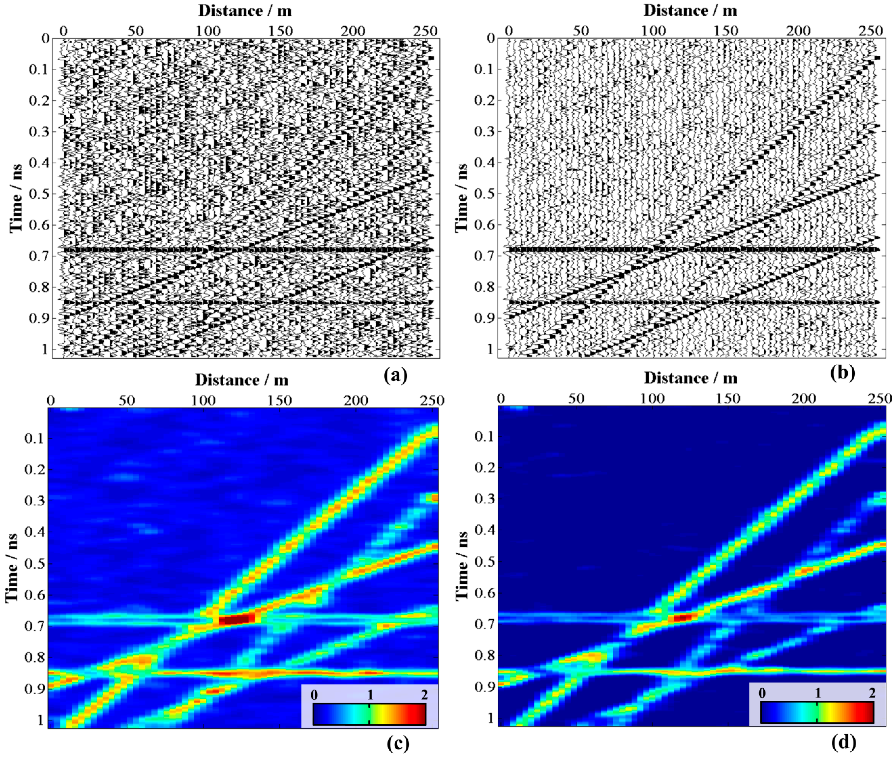
In Figure 5, we add noise with different noise levels into the same data (Figure 4a) to obtain two noisy datasets with similar useful signal (Figure 5a,b). The added noise is Gaussian random noise and the distribution is and , respectively. Then, we calculate the similarity spectrum (Figure 5c) between the two noisy data and apply a soft threshold function to it. In this spectrum, we observe a large similarity difference between signal and noise. After the soft thresholding, the spectrum highlights the useful signal.
According to the property of local similarity, we propose a rock-extracting method based on local similarity constraint. The detailed workflow is shown as follows:
- (1)
- For LPR CH-2A and B data
- (a)
- Apply a preprocessing line.
- (b)
- Attenuate steep-dip components by an f-x EMD-based low-pass dip filter.
- (2)
- Calculate local similarity spectrum between LPR CH-2A and B data.
- (3)
- Utilize a soft threshold function for the local similarity spectrum.
- (4)
- Mute the reflection area.
- (5)
- Pick the local maximum and record the corresponding space coordinates.
3. Results
3.1. Verification of Simulation Result
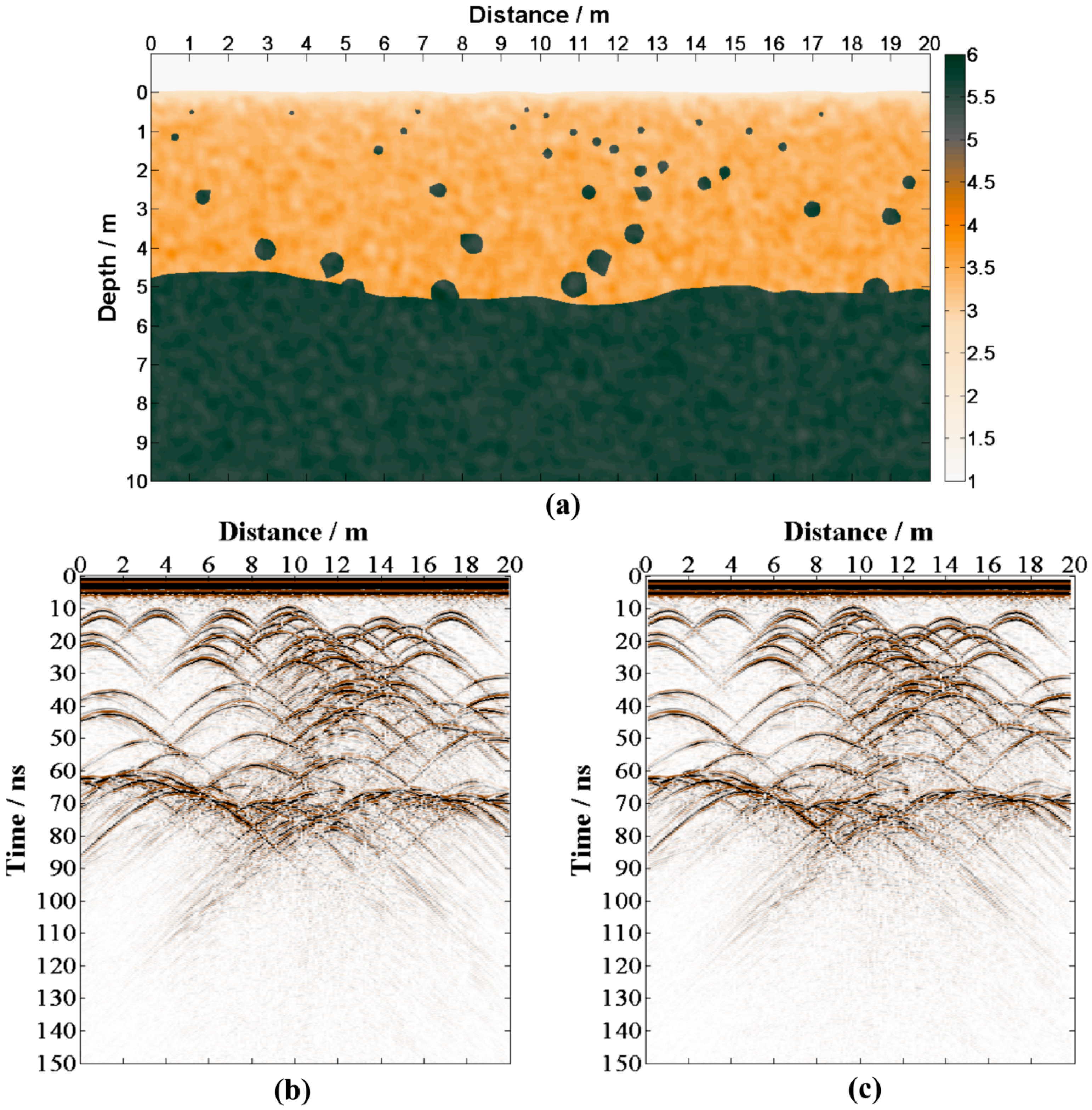
In order to validate the effectiveness of the proposed method, a complex model (Figure 6a) is built. This synthetic model considers many factors referenced from [24,25,26]: random medium, undulating interface, and anomalous body. FDTD is applied for the simulation of the simple model [27]. According to the actual acquisition parameters of LPR [2], the simulated parameters are shown in Table 2. The forward results are obtained in Figure 6b,c.
In the forward results (Figure 5b,c), there are two types of useful signals, i.e., reflections (0–6 and 60–80 ns) and diffractions (10–60 ns). Since our focus is rock positioning, we mute the shallow reflections before the dip filter.
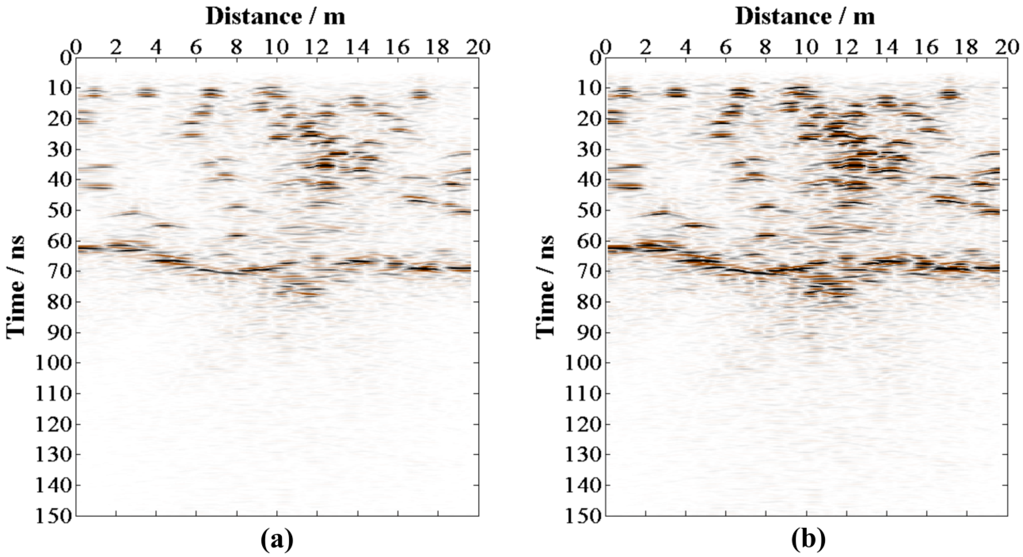
Figure 7 demonstrates the results of the dip filter. After the f-x EMD-based low-pass dip filter, the steep-dip components are well attenuated. For diffractions, the positions of filtered components are consistent with their corresponding vertex positions. We also see some noise residual in the filtered data, leading to many noise-caused local maximums.
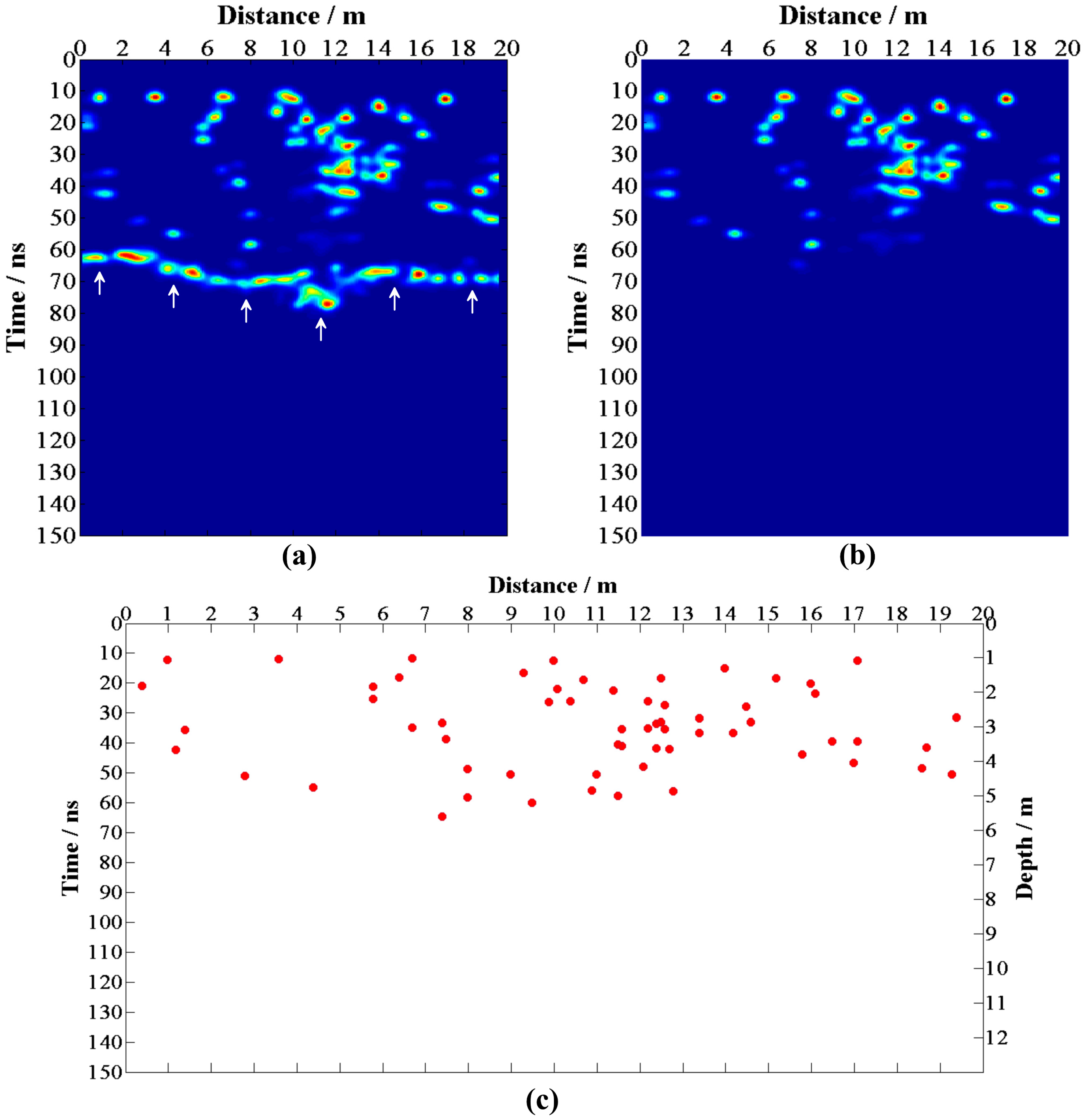
Figure 8 demonstrates the local similarity spectrum between the two filtered datasets after soft thresholding and the result of rock positioning. The spectrum is clean and signal-dominated, proving the effectiveness of our method; the energy group denotes the useful signal. Note that reflection energy in the spectrum also leads to unexpected rock extraction. Before local maximum picking, we mute the deep reflection energy (arrows in Figure 8a) and the muted results are shown in Figure 8b. Figure 8c demonstrates the result of rock positioning.
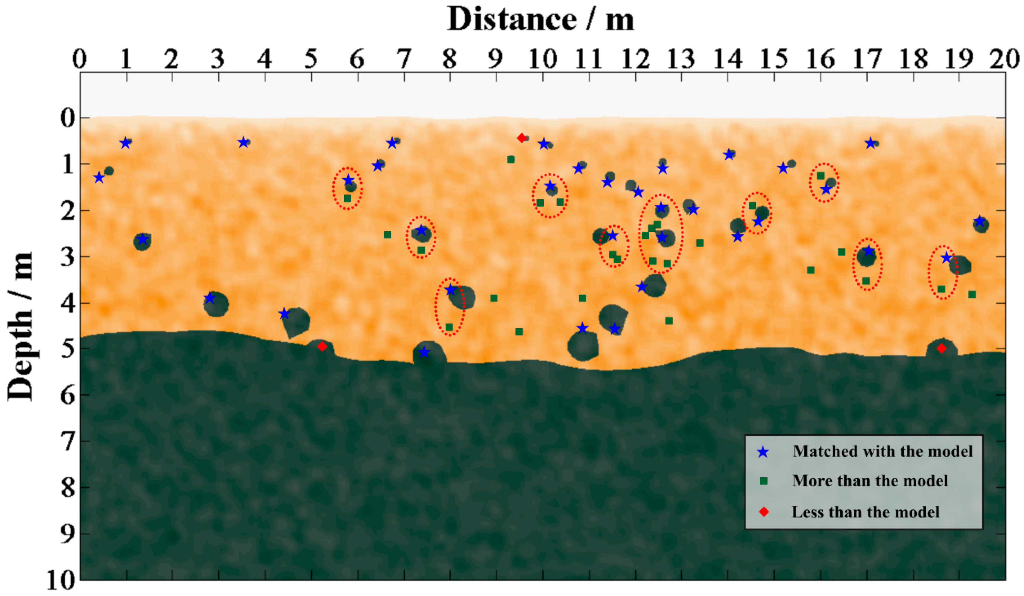
In order to evaluate the effect of rock positioning, we compare the result with the integrated regolith model (Figure 6a). From Figure 9, we see that most of the rocks are effectively extracted and their position is consistent with the model and a few rocks are unextracted and over extracted.
We use three concepts (detection rate, missed detection rate and false alarm rate) to evaluate the result of rock positioning quantitatively.
(1) The detection rate is the probability that a rock block can be detected and is expressed by:
where is the number of the rocks which can be detected, is the total number of rocks.
(2) The rate of missed detection is the probability that a rock block cannot be detected. It is expressed by:
where is the number of the rocks which cannot be detected, is the total number of rocks.
(3) The false alarm rate is the probability that a non-existent rock is detected. It is expressed by:
where is the number of the detected rocks which are non-existent, is the total number of rocks.
The detection rate of the above-mentioned forward result is , the missed detection rate is , and the false alarm rate is . It can be seen that our method has a high detection rate and a low missed detection rate. The reason for missed detection is that the rock is close to the reflector so that the diffractions are interfered with by reflections. The false alarm rate is relatively high; there are two main reasons for the excessive extraction of rocks: (1) In the rock enrichment area (9–13 m), diffraction interferences decrease the accuracy of local maximum picking; (2) bigger rocks allow the diffractions generated by their upper and lower interfaces to be recognized, which generates serval “rock pairs” (red circle) in extracted results. After removing these “rock pairs”, the actual false alarm rate drops to . Although there are a few errors in the extraction results, the rock distribution is close to the model, which is acceptable for the rock analysis.
3.2. LPR Data Result
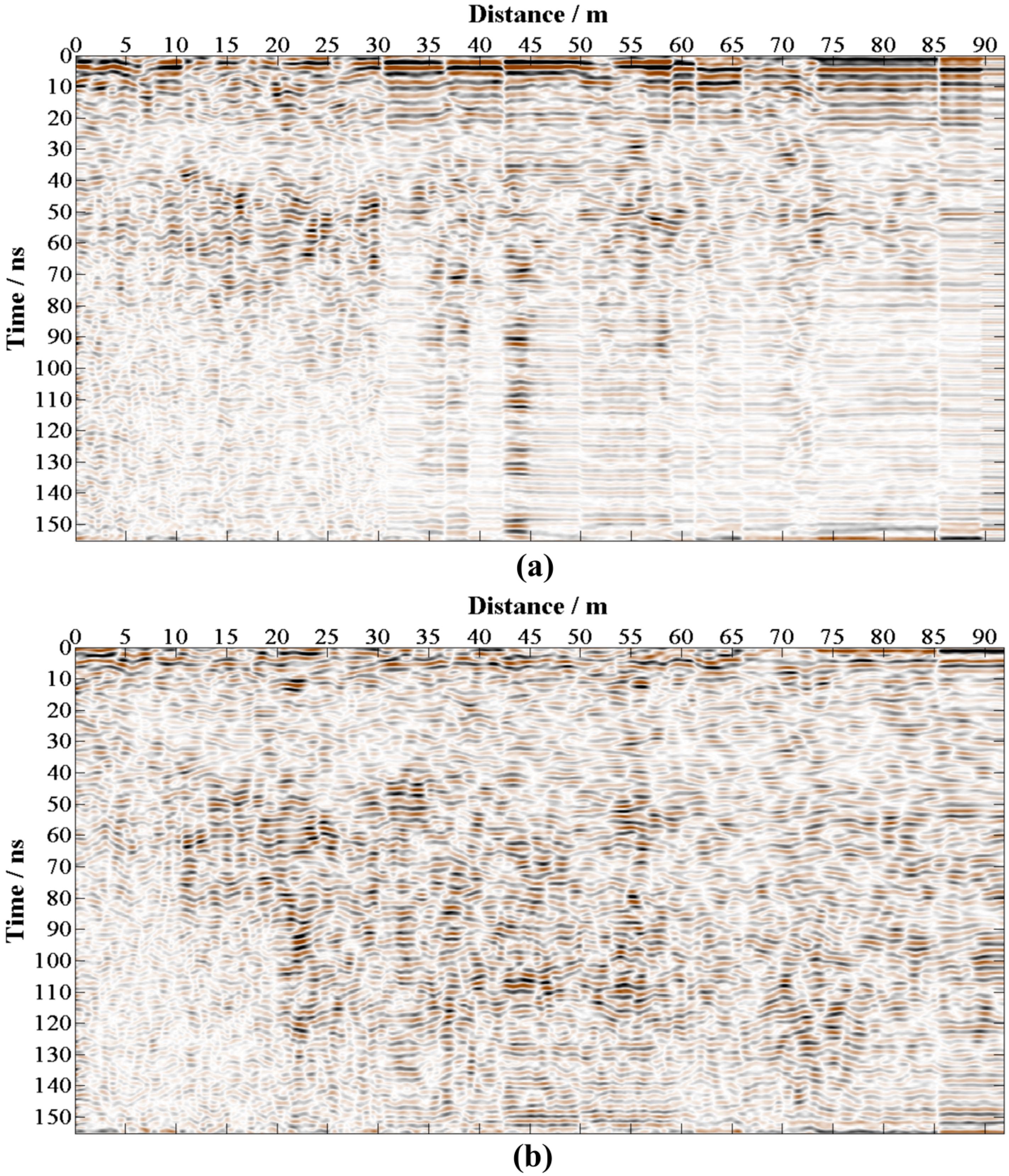
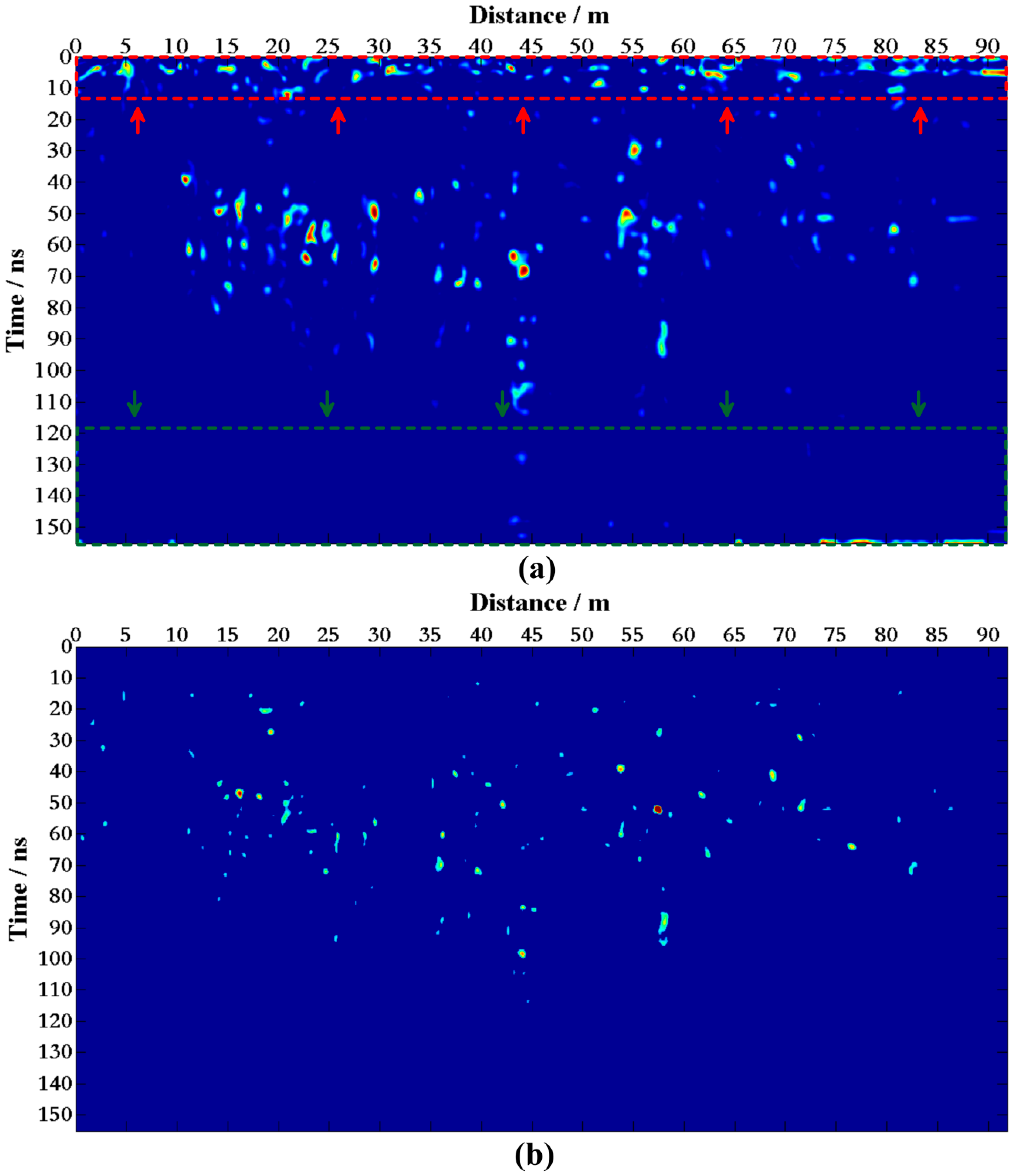
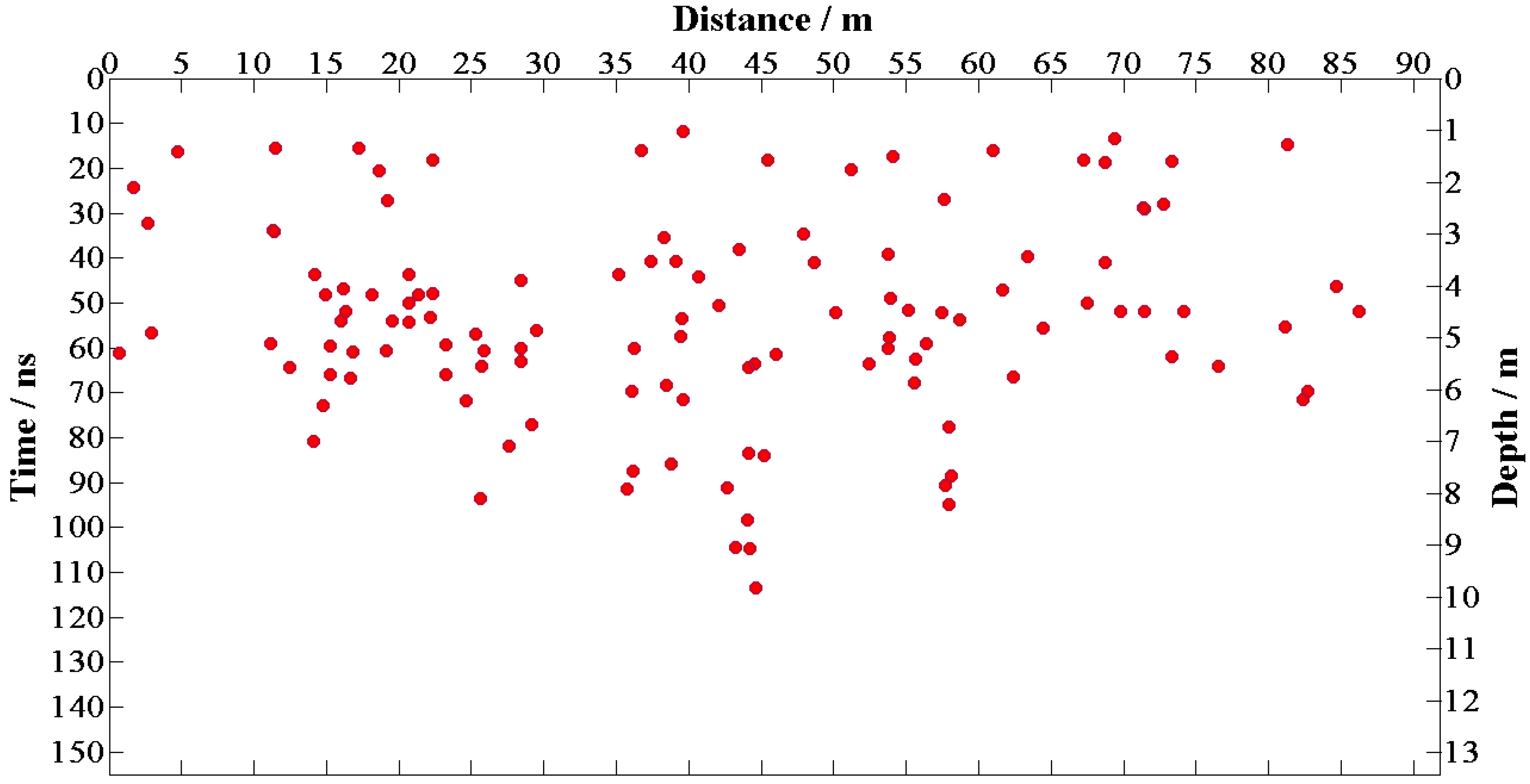
After proving the effectiveness of our proposed method, we process the LPR CH-2 data. The results of the dip filter are shown in Figure 10 and the corresponding local similarity spectra are shown in Figure 11a. From Figure 10, we see that most diffractions locate in 15–118 ns. The muted spectrum is shown in Figure 11b. Then, we utilize the result of rock positioning (Figure 12) to research the evolution of regolith on the landing site.
4. Discussion
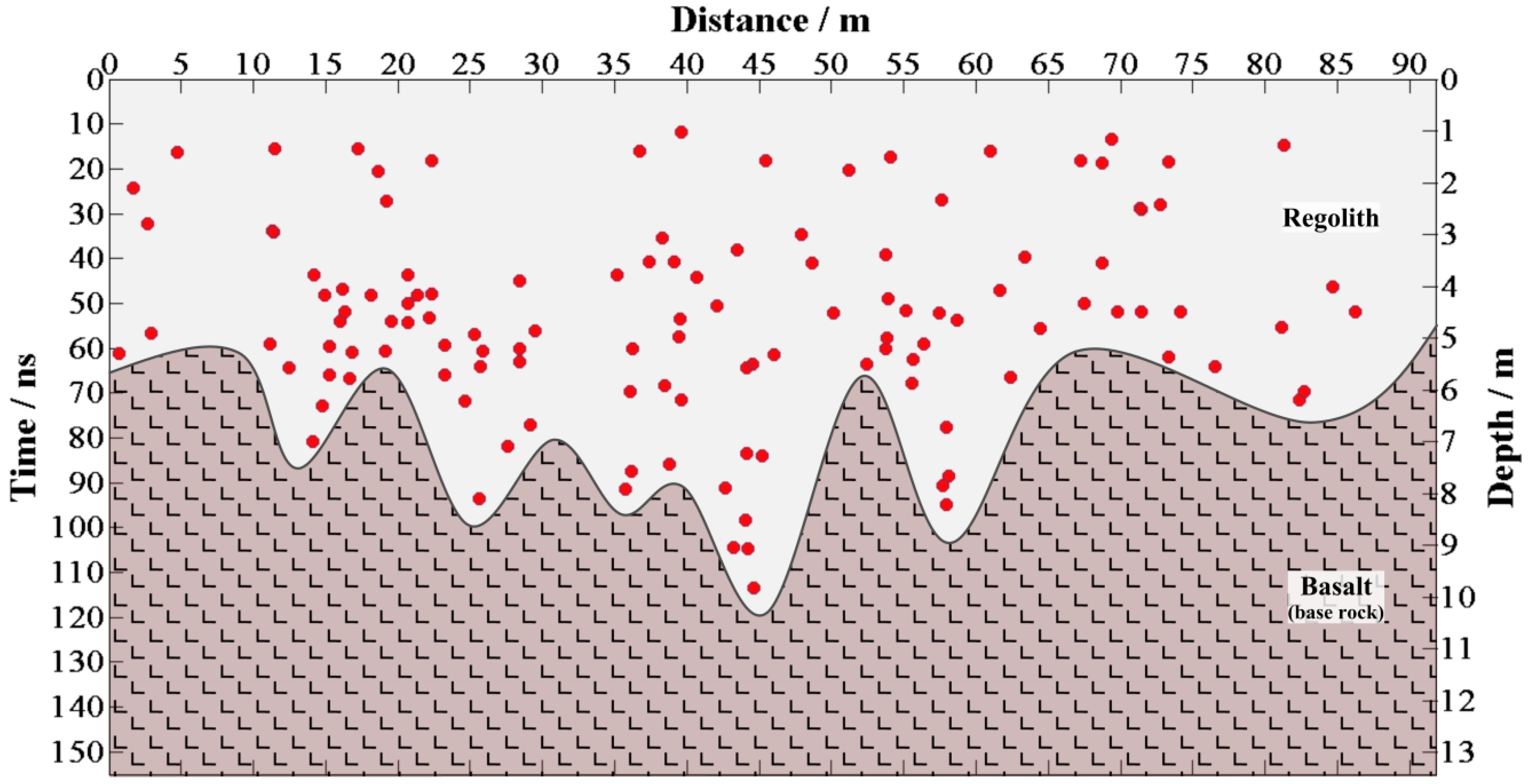
After we obtained the result of rock positioning for LPR data, we divided the layers according to the distribution of the rocks, as shown in Figure 13. The base rock layer is basalt, which is the product of the last basalt covering. The regolith layer contains a lot of rock fragments. The depth of regolith is 5 m at minimum and 10 m at maximum. The stratified result is consistent with previous results [5,6,7].
The dielectric constant is critical for time-depth conversion. The permittivity of lunar regolith is influenced by density and ilmenite concentrations [28,29,30]. Many measurements have been investigated using lunar regolith samples from the Apollo & Luna era; the relative dielectric constant of Surveyor regolith samples ranges from 2.00 to 3.28 [31] and the relative dielectric constant of Luna regolith samples ranges from 1.7 to 4.4 [32,33]. More recently, microwave remote sensing was used to estimate the dielectric constant of regolith [34,35]. Fa et al., Dong et al. and Feng et al. report the estimated results of the lunar regolith permittivity in the CE-3 landing area using the LPR are 3.0 ± 0.03, 2.9 ± 0.4 and ~3, respectively [5,8,36]. Therefore, we set the relative dielectric constant to 3.0 as an appropriate value for time-depth conversion in the processing pipeline (Figure 3).
To estimate the depth error, we need to set the range of the dielectric constant. Based on previous research results [5,8,36] and including all dielectric constant estimates, we believe that is a suitable range of dielectric constant variation. After counting and analysing the extracted rocks, we obtain their space location, time, and depth position (Appendix C) for different dielectric constants (). When , the error of the position estimation is less than 10% (−9.62% to 7.36%), and the maximum error values are −0.87 and 0.67 m. In the same way, we estimate the position of the interface. When , the average estimated depth of lunar regolith is estimated to be m.
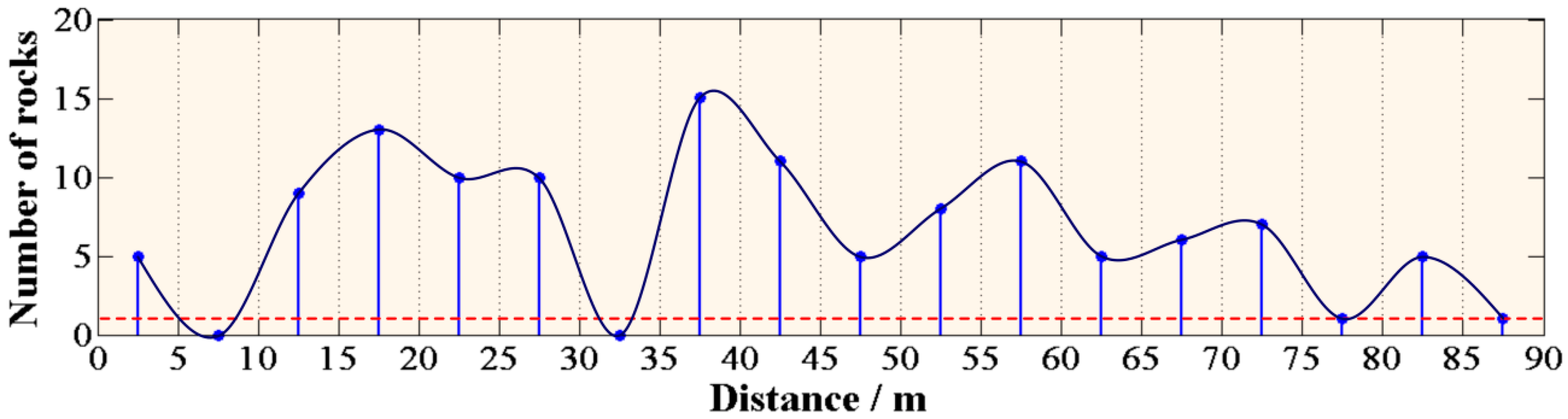
Moreover, we can also obtain the distribution information of the rocks in regolith which changes with the path and the depth. Figure 14 is a scatterplot of the rock number and location at each 5 m. The figure shows us a relationship between the number of rocks and distance. There is a minimum value at 5–10 m, 30–35 m, 75–80 m and 85–90 m where the number is less than 1. The Chang’E-5 mission will drill and collect the regolith from the moon [37], which requires that there is no rock below the drilling point, otherwise the drilling machine will be damaged. The scatterplot can help us select the drilling point.
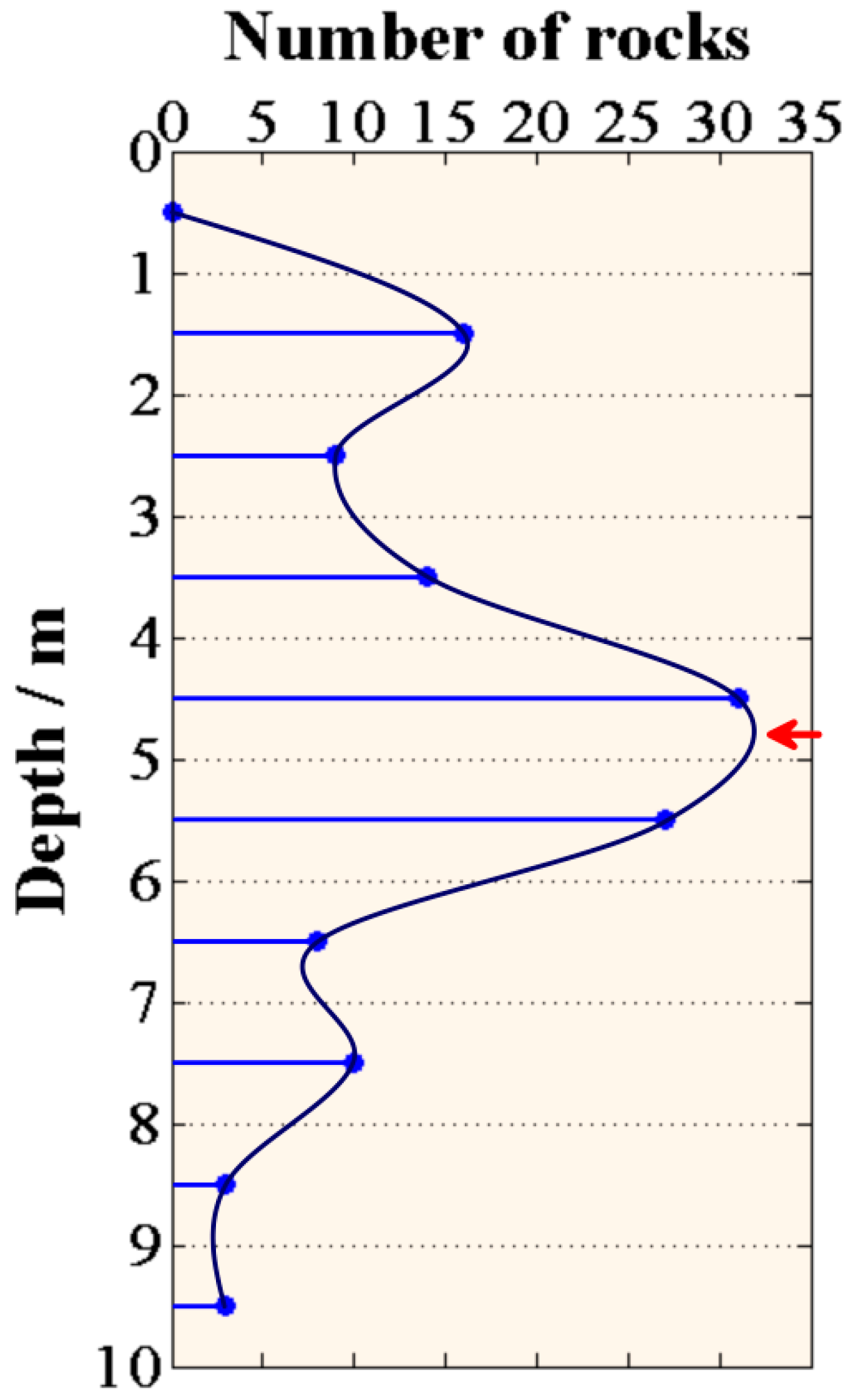
In the same way, the analysis between the number of rocks and depth has been performed in Figure 15. There is a maximum value at ~5 m. The above stratified analysis tells us that the depth of regolith is 5 m at minimum and 10 m at maximum. From 5 m, the interface appears, and the number of rocks is decreasing. The tendency in Figure 15 is consistent with the stratigraphic structure at the CE-3 landing site.
5. Conclusions
The LPR equipped on the Yutu Rover detected the lunar geological structure in the Northern Imbrium. A data preprocessing pipeline is designed to solve some types of issues, such as repeated and waste traces and noise. Then, we propose an adaptive rock positioning method based on local similarity constraint, which utilizes the similarity between LPR CH-2A and B data. This method is implemented in two steps, namely, low-wavenumber component extraction and noise-caused local maximum attenuation. Finally, according to the extracted result, on the one hand, the depth of regolith is obtained, and on the other hand, the distribution information of the rocks in regolith, which changes with the path and the depth, is also revealed.
The position of each rock and the contact interface of regolith are still difficult to recognize. We adopt an f-x EMD-based dip filter to extract low-wavenumber components from the two data sets. Then, we calculate the local similarity spectrum between the filtered CH-2 A and B. After a soft threshold function, we pick the local maximums in the spectrum as the location of each rock.
The result of rock positioning for LPR data helps us to divide the layers according to the distribution of the rocks. The base rock layer is basalt, which is the product of the last basalt covering. The regolith layer contains a lot of rock fragments. The depth of regolith is 5 m at minimum and 10 m at maximum. The analysis of the rock number and location provides a priori information for the further CE-5 plan of regolith collection. The analysis between the number of rocks and depth is consistent with the stratigraphic structure at the CE-3 landing site.
These results provide valuable information regarding our understanding of the modification of the lunar surface and the evolution of the regolith, and the results are also important as a reference for future lunar sample return missions.
Author Contributions
L.Z. and B.H. conceived and designed the study. D.W. designed the processing workflow. Z.Z. provided the idea. B.H. processed the LPR data and L.Z. interpreted the results. B.H. wrote the paper.
Funding
This work was supported by the Major Projects of the National Science and Technology of China (Grant No. 2016ZX05026-002-003), the National Natural Science Foundation of China (41374108, 41574097 and 41504083), the National Key Research Development Program (2016YC06001104) and the Graduate Innovation Fund of Jilin University.
Acknowledgments
We thank Madagascar software for the open-source code and the open-source data in http://moon.bao.ac.cn.
Conflicts of Interest
The funders had no role in the design of the study; in the collection, analyses, or interpretation of data; in the writing of the manuscript, or in the decision to publish the results.
Appendix A

Table A1.
IDs of the LPR data.
| IDs |
|---|
| CE3_BMYK_LPR-2A_SCI_N_20091231160000_20131215171000_0001_A.2B |
| CE3_BMYK_LPR-2A_SCI_N_20131215171001_20131220141300_0002_A.2B |
| CE3_BMYK_LPR-2A_SCI_N_20131220141301_20131220181800_0003_A.2B |
| CE3_BMYK_LPR-2A_SCI_N_20131220181801_20131221124500_0004_A.2B |
| CE3_BMYK_LPR-2A_SCI_N_20131221124501_20131223174500_0005_A.2B |
| CE3_BMYK_LPR-2A_SCI_N_20131223174501_20131226000000_0006_A.2B |
| CE3_BMYK_LPR-2A_SCI_N_20131226000001_20140112193800_0007_A.2B |
| CE3_BMYK_LPR-2A_SCI_N_20140112193801_20140114213300_0008_A.2B |
| CE3_BMYK_LPR-2A_SCI_N_20140114213301_20140124000000_0009_A.2B |
| CE3_BMYK_LPR-2B_SCI_N_20091231160000_20131215171000_0001_A.2B |
| CE3_BMYK_LPR-2B_SCI_N_20131215171001_20131220141300_0002_A.2B |
| CE3_BMYK_LPR-2B_SCI_N_20131220141301_20131220181800_0003_A.2B |
| CE3_BMYK_LPR-2B_SCI_N_20131220181801_20131221124500_0004_A.2B |
| CE3_BMYK_LPR-2B_SCI_N_20131221124501_20131223174500_0005_A.2B |
| CE3_BMYK_LPR-2B_SCI_N_20131223174501_20131226000000_0006_A.2B |
| CE3_BMYK_LPR-2B_SCI_N_20131226000001_20140112193800_0007_A.2B |
| CE3_BMYK_LPR-2B_SCI_N_20140112193801_20140114213300_0008_A.2B |
| CE3_BMYK_LPR-2B_SCI_N_20140114213301_20140124000000_0009_A.2B |
Appendix B
Review of Local Similarity
The local similarity between two vectors can be defined as:
where and are obtained by solving the optimization problem in the least squares sense:
where and represent diagonal matrices whose main diagonal elements are and , respectively, and represents a diagonal matrix whose main diagonal element is .
Local smoothness estimation is introduced as a constraint for shaping regularization. The optimization problem in the least squares sense can be modified as follows:
where is a function for smoothness promotion, and and are the two stable parameters used in the process of inversion to accelerate the convergence speed. We can select and as follows:
Appendix C
Table A2.
Rock depth with different dielectric constants.
| Rock Number | Distance/m | Time/ns | Error/m | ||||
|---|---|---|---|---|---|---|---|
| 1 | 0.68 | 61.56 | 5.81 | 5.30 | 4.91 | −0.51 | 0.39 |
| 6 | 11.14 | 59.38 | 5.60 | 5.11 | 4.74 | −0.49 | 0.38 |
| 11 | 14.14 | 81.25 | 7.67 | 7.01 | 6.49 | −0.67 | 0.52 |
| 16 | 15.24 | 66.25 | 6.25 | 5.71 | 5.29 | −0.55 | 0.42 |
| 21 | 16.86 | 61.25 | 5.78 | 5.28 | 4.89 | −0.50 | 0.39 |
| 26 | 19.26 | 27.50 | 2.58 | 2.35 | 2.18 | −0.22 | 0.17 |
| 31 | 21.38 | 48.44 | 4.57 | 4.17 | 3.86 | −0.40 | 0.31 |
| 36 | 23.28 | 59.69 | 5.63 | 5.14 | 4.76 | −0.49 | 0.38 |
| 41 | 25.86 | 60.94 | 5.75 | 5.25 | 4.86 | −0.50 | 0.39 |
| 46 | 29.22 | 77.50 | 7.32 | 6.68 | 6.19 | −0.64 | 0.50 |
| 51 | 36.16 | 87.81 | 8.30 | 7.58 | 7.02 | −0.72 | 0.56 |
| 56 | 38.48 | 68.75 | 6.49 | 5.93 | 5.49 | −0.57 | 0.44 |
| 61 | 39.64 | 71.88 | 6.79 | 6.20 | 5.74 | −0.59 | 0.46 |
| 66 | 43.26 | 104.69 | 9.90 | 9.04 | 8.37 | −0.86 | 0.67 |
| 71 | 44.24 | 105.00 | 9.93 | 9.07 | 8.39 | −0.87 | 0.67 |
| 76 | 46.04 | 61.88 | 5.84 | 5.33 | 4.94 | −0.51 | 0.40 |
| 81 | 52.44 | 63.75 | 6.02 | 5.49 | 5.09 | −0.52 | 0.41 |
| 86 | 54.12 | 17.81 | 1.66 | 1.52 | 1.40 | −0.14 | 0.11 |
| 91 | 57.50 | 52.50 | 4.95 | 4.52 | 4.18 | −0.43 | 0.34 |
| 96 | 58.10 | 88.75 | 8.39 | 7.66 | 7.09 | −0.73 | 0.57 |
| 101 | 63.42 | 40.00 | 3.77 | 3.44 | 3.18 | −0.33 | 0.25 |
| 106 | 68.74 | 19.06 | 1.78 | 1.62 | 1.50 | −0.15 | 0.12 |
| 111 | 71.48 | 52.19 | 4.92 | 4.49 | 4.16 | −0.43 | 0.33 |
| 116 | 76.58 | 64.38 | 6.08 | 5.55 | 5.14 | −0.53 | 0.41 |
| 121 | 84.74 | 46.56 | 4.39 | 4.01 | 3.71 | −0.38 | 0.30 |
References
- Xiao, L.; Zhu, P.; Fang, G.; Xiao, Z.; Zou, Y.; Zhao, J.; Zhao, N.; Yuan, Y.; Qiao, L.; Zhang, X.; et al. A young multilayered terrane of the northern Mare Imbrium revealed by Chang’E-3 mission. Science 2015, 347, 1226–1229. [Google Scholar] [CrossRef] [PubMed]
- Fang, G.Y.; Zhou, B.; Ji, Y.C.; Zhang, Q.Y.; Shen, S.X.; Li, Y.X.; Guan, H.F.; Tang, C.J.; Gao, Y.Z.; Lu, W.; et al. Lunar Penetrating Radar onboard the Chang’e-3 mission. Res. Astron. Astrophys. 2014, 14, 1607–1622. [Google Scholar] [CrossRef]
- Su, Y.; Fang, G.Y.; Feng, J.Q.; Xing, S.G.; Ji, Y.C.; Zhou, B.; Gao, Y.Z.; Li, H.; Dai, S.; Xiao, Y.; et al. Data processing and initial results of Chang’e-3. lunar penetrating radar. Res. Astron. Astrophys. 2014, 14, 1623–1632. [Google Scholar] [CrossRef]
- Zhang, J.; Yang, W.; Hu, S.; Lin, Y.; Fang, G.; Li, C.; Peng, W.; Zhu, S.; He, Z.; Zhou, B.; et al. Volcanic history of the Imbrium basin: A close-up view from the lunar rover Yutu. Proc. Natl. Acad. Sci. USA 2015, 112, 5342–5347. [Google Scholar] [CrossRef] [PubMed] [Green Version]
- Fa, W.; Zhu, M.H.; Liu, T.; Plescia, J.B. Regolith stratigraphy at the Chang’E-3 landing site as seen by lunar penetrating radar. Geophys. Res. Lett. 2015, 16, 10–79. [Google Scholar] [CrossRef]
- Lai, J.; Xu, Y.; Zhang, X.; Tang, Z. Structural analysis of lunar subsurface with Chang’E-3 lunar penetrating radar. Planet. Space Sci. 2016, 120, 96–102. [Google Scholar] [CrossRef]
- Zhang, L.; Zeng, Z.; Li, J.; Huang, L.; Huo, Z.; Zhang, J.; Huai, N. A Story of Regolith Told by Lunar Penetrating Radar. Icarus 2019, 321, 148–160. [Google Scholar] [CrossRef]
- Dong, Z.; Fang, G.; Ji, Y.; Gao, Y.; Zhang, X. Parameters and structure of lunar regolith in chang’e-3 landing area from lunar penetrating radar (lpr) data. Icarus 2016, 282, 40–46. [Google Scholar] [CrossRef]
- Zhang, L.; Zeng, Z.; Li, J.; Huang, L.; Huo, Z.; Wang, K.; Zhang, J. Parameter Estimation of Lunar Regolith from Lunar Penetrating Radar Data. Sensors 2018, 18, 2907. [Google Scholar] [CrossRef] [PubMed]
- Trorey, A. A simple theory for seismic diffractions. Geophysics 1970, 35, 1961–1983. [Google Scholar] [CrossRef]
- Bazelaire, E. Normal moveout revisited: Inhomogeneous media and curved interfaces. SEG Tech. Program Expand. Abstr. 1986, 5, 403. [Google Scholar]
- Huang, N.; Shen, Z.; Long, S.; Wu, M.; Shih, H.; Zheng, Q. The empirical mode decomposition and the hilbert spectrum for nonlinear and non-stationary time series analysis. Proc. R. Soc. A Math. Phys. Eng. Sci. 1998, 454, 903–995. [Google Scholar] [CrossRef]
- Maïza, B.; Baan, M. Random and coherent noise attenuation by empirical mode decomposition. Geophysics 2009, 74, 89–98. [Google Scholar]
- Cai, H.; He, Z.; Huang, D. Seismic data denoising based on mixed time-frequency methods. Appl. Geophys. 2011, 8, 319–327. [Google Scholar] [CrossRef]
- Chen, Y.; Ma, J. Random noise attenuation by f-x empirical-mode decomposition predictive filtering. Geophysics 2014, 79, 81–91. [Google Scholar] [CrossRef]
- Fomel, S. Local seismic attributes. Geophysics 2007, 72, 29–33. [Google Scholar] [CrossRef]
- Fomel, S. Shaping regularization in geophysical-estimation problems. Geophysics 2007, 24, 29–36. [Google Scholar] [CrossRef]
- Liu, G.; Fomel, S.; Jin, L.; Chen, X. Stacking seismic data using local correlation. Geophysics 2009, 74, 43–48. [Google Scholar] [CrossRef]
- Liu, G.; Fomel, S.; Chen, X. Time-frequency characterization of seismic data using local attributes. Geophysics 2009, 76, 23–24. [Google Scholar] [CrossRef]
- Chen, Y.; Jiao, S.; Ma, J.; Chen, H.; Zhou, Y.; Gan, S. Ground-roll noise attenuation using a simple and effective approach based on local band-limited orthogonalization. IEEE Geosci. Remote Sens. Lett. 2015, 12, 2316–2320. [Google Scholar] [CrossRef]
- Chen, Y.; Fomel, S. Random noise attenuation using local signal-and-noise orthogonalization. Geophysics 2015, 80, 23–24. [Google Scholar] [CrossRef]
- Chen, Y. Iterative deblending with multiple constraints based on shaping regularization. IEEE Geosci. Remote Sens. Lett. 2015, 12, 2247–2251. [Google Scholar] [CrossRef]
- Bekara, M.; van der Baan, M. Local singular value decomposition for signal enhancement of seismic data. Geophysics 2007, 72, 59–65. [Google Scholar] [CrossRef]
- Zhang, L.; Zeng, Z.; Li, J.; Lin, J.; Hu, Y.; Wang, X.; Sun, X. Simulation of the Lunar Regolith and Lunar-Penetrating Radar Data Processing. IEEE J. Sel. Top. Appl. Earth Observ. Remote Sens. 2018, 11, 655–663. [Google Scholar] [CrossRef]
- Zhang, L.; Zeng, Z.F.; Li, J.; Lin, J.Y. Study on regolith modeling and lunar penetrating radar simulation. In Proceedings of the 2016 16th International Conference on Ground Penetrating Radar (GPR), Hong Kong, China, 13–16 June 2016. [Google Scholar]
- Li, J.; Zeng, Z.; Liu, C.; Huai, N.; Wang, K. A Study on Lunar Regolith Quantitative Random Model and Lunar Penetrating Radar Parameter Inversion. IEEE Geosci. Remote Sens. Lett. 2017, 14, 1953–1957. [Google Scholar] [CrossRef]
- Irving, J.; Knight, R. Numerical modeling of ground-penetrating radar in 2-D using MATLAB. Comput. Geosci. 2006, 32, 1247–1258. [Google Scholar] [CrossRef]
- Olhoeft, G.; Strangway, D. Dielectric properties of the first 100 meters of the Moon. Earth Planet. Sci. Lett. 1975, 24, 394–404. [Google Scholar] [CrossRef]
- Ulaby, F.; Bengal, T.; Dobson, M.; East, J.R.; Garvin, J.B.; Evans, D.L. Microwave dielectric properties of dry rocks. IEEE Trans. Geosci. Remote Sens. 1990, 28, 325–336. [Google Scholar] [CrossRef]
- Carrier, W.; Olhoeft, G.; Mendell, W. Physical Properties of the Lunar Surface; Cambridge University Press: Cambridge, UK, 1991; pp. 530–552. [Google Scholar]
- Muhleman, D.; Brown, W.; Davids, L. Lunar surface electromagnetic properties. NASA 1969, 184, 203–269. [Google Scholar]
- Kroupenio, N. Some characteristics of the Venus surface. Icarus 1972, 17, 692–698. [Google Scholar] [CrossRef]
- Kroupenio, N. Results of radar experiments performed on automatic stations Luna 16 and Luna 17. In Proceedings of the COSPAR Space Research XIII, Madrid, Spain, 10 May 1972; pp. 969–973. [Google Scholar]
- Shkuratov, Y.; Bondarenko, N. Regolith layer thickness mapping of the moon by radar and optical data. Icarus 2001, 149, 329–338. [Google Scholar] [CrossRef]
- Fa, W.; Jin, Y. A primary analysis of microwave brightness temperature of lunar surface from chang-e 1 multi-channel radiometer observation and inversion of regolith layer thickness. Icarus 2010, 207, 605–615. [Google Scholar] [CrossRef]
- Feng, J.; Su, Y.; Ding, C. Dielectric properties estimation of the lunar regolith at CE-3 landing site using lunar penetrating radar data. Icarus 2016, 284, 424–430. [Google Scholar] [CrossRef]
- Li, Y.; Lu, W.; Fang, G.; Shen, S. The Imaging Method and Verification Experiment of Chang’E-5 Lunar Regolith Penetrating Array Radar. IEEE Geosci. Remote Sens. Lett. 2018, 15, 1006–1010. [Google Scholar] [CrossRef]
Figure 1.
Yutu’s path on the Moon. The context image was taken by the descent camera on the CE-3 lander. The red star shows the landing site. The blue line shows the path.
Figure 1.
Yutu’s path on the Moon. The context image was taken by the descent camera on the CE-3 lander. The red star shows the landing site. The blue line shows the path.

Figure 2.
(a) The position of CH-2 antenna on the rover (b) The structure of the CH2 antenna.

Figure 3.
A pipeline chart of CH-2 LPR data processing. N103-N209 denote the positions.

Figure 4.
Demonstration of dip filter using f-x EMD. (a) The synthetic data, (b) high-pass dip filtered data, (c) mid-pass dip filtered data, (d) low-pass dip filtered data.
Figure 4.
Demonstration of dip filter using f-x EMD. (a) The synthetic data, (b) high-pass dip filtered data, (c) mid-pass dip filtered data, (d) low-pass dip filtered data.

Figure 5.
(a) Noisy data with , (b) Noisy data with , (c) Local similarity between (a) and (b), (d) Local similarity spectrum after soft thresholding.
Figure 5.
(a) Noisy data with , (b) Noisy data with , (c) Local similarity between (a) and (b), (d) Local similarity spectrum after soft thresholding.

Figure 6.
(a) The synthetical regolith model, (b) Forward result A with offset of 0.16 m (c) Forward result B with offset of 0.32 m.
Figure 6.
(a) The synthetical regolith model, (b) Forward result A with offset of 0.16 m (c) Forward result B with offset of 0.32 m.

Figure 7.
Demonstration of dip filter results in two datasets with different offsets.

Figure 8.
(a) Local similarity spectrum in two filtered datasets (Figure 6), (b) diffraction section of (a), (c) the result of rock positioning
Figure 8.
(a) Local similarity spectrum in two filtered datasets (Figure 6), (b) diffraction section of (a), (c) the result of rock positioning

Figure 9.
The comparison of rock positioning.

Figure 10.
The results of the dip filter for (a) LPR CH-2A data and (b) LPR CH-2B data.

Figure 11.
(a) Local similarity spectrum for filtered LPR CH-2A and B, (b) diffraction section of (a).
Figure 11.
(a) Local similarity spectrum for filtered LPR CH-2A and B, (b) diffraction section of (a).

Figure 12.
The result of rock positioning for LPR data. The relative dielectric constant is set to 3.
Figure 12.
The result of rock positioning for LPR data. The relative dielectric constant is set to 3.

Figure 13.
The interface of regolith and base rock. The relative dielectric constant is set to 3.

Figure 14.
Scatterplot of the rock number and location at each 5 m.

Figure 15.
Analysis between the number of rocks and depth.

Table 1.
Parameter list for three types of dip filters.
| Type | N | m | ||
|---|---|---|---|---|
| High-pass | 6 | 2 | , | |
| Mid-pass | 6 | 3 | , , | |
| Low-pass | 6 | 2 | , |
Table 2.
Simulation Parameter.
| Result A | Result B | |
|---|---|---|
| Height | 0.3 m | |
| Offset | 0.16m | 0.32m |
| Center frequency | 500MHz | |
| Wavelet | Ricker | |
| Absorbing boundary | C-PML | |
| Discrete grid | 0.005 m * 0.005 m | |
| Time step | 0.040434 ns | |
| Time window | 120 ns | |
| Random access memory | 8.00 GB | |
| Central Processing Unit | Intel(R) Core (TM) i5-4590 CPU @3.30GHz | |
| Time | 24.7699 h | 24.8101 h |
© 2019 by the authors. Licensee MDPI, Basel, Switzerland. This article is an open access article distributed under the terms and conditions of the Creative Commons Attribution (CC BY) license (http://creativecommons.org/licenses/by/4.0/).
Share and Cite
MDPI and ACS Style
Hu, B.; Wang, D.; Zhang, L.; Zeng, Z. Rock Location and Quantitative Analysis of Regolith at the Chang’e 3 Landing Site Based on Local Similarity Constraint. Remote Sens. 2019, 11, 530. https://0-doi-org.brum.beds.ac.uk/10.3390/rs11050530
AMA Style
Hu B, Wang D, Zhang L, Zeng Z. Rock Location and Quantitative Analysis of Regolith at the Chang’e 3 Landing Site Based on Local Similarity Constraint. Remote Sensing. 2019; 11(5):530. https://0-doi-org.brum.beds.ac.uk/10.3390/rs11050530
Chicago/Turabian StyleHu, Bin, Deli Wang, Ling Zhang, and Zhaofa Zeng. 2019. "Rock Location and Quantitative Analysis of Regolith at the Chang’e 3 Landing Site Based on Local Similarity Constraint" Remote Sensing 11, no. 5: 530. https://0-doi-org.brum.beds.ac.uk/10.3390/rs11050530
Note that from the first issue of 2016, this journal uses article numbers instead of page numbers. See further details here.