Mapping Coastal Wetland Biomass from High Resolution Unmanned Aerial Vehicle (UAV) Imagery


Department of Geography, University of California, Los Angeles, Los Angeles, CA 90095, USA
*
Author to whom correspondence should be addressed.
Remote Sens. 2019, 11(5), 540; https://0-doi-org.brum.beds.ac.uk/10.3390/rs11050540
Submission received: 31 January 2019
/
Revised: 1 March 2019
/
Accepted: 2 March 2019
/
Published: 6 March 2019
(This article belongs to the Special Issue Satellite-Based Wetland Observation)
Abstract
:Salt marsh productivity is an important control of resiliency to sea level rise. However, our understanding of how marsh biomass and productivity vary across fine spatial and temporal scales is limited. Remote sensing provides a means for characterizing spatial and temporal variability in marsh aboveground biomass, but most satellite and airborne sensors have limited spatial and/or temporal resolution. Imagery from unmanned aerial vehicles (UAVs) can be used to address this data gap. We combined seasonal field surveys and multispectral UAV imagery collected using a DJI Matrice 100 and Micasense Rededge sensor from the Carpinteria Salt Marsh Reserve in California, USA to develop a method for high-resolution mapping of aboveground saltmarsh biomass. UAV imagery was used to test a suite of vegetation indices in their ability to predict aboveground biomass (AGB). The normalized difference vegetation index (NDVI) provided the strongest correlation to aboveground biomass for each season and when seasonal data were pooled, though seasonal models (e.g., spring, r2 = 0.67; RMSE = 344 g m−2) were more robust than the annual model (r2 = 0.36; RMSE = 496 g m−2). The NDVI aboveground biomass estimation model (AGB = 2428.2 × NDVI + 120.1) was then used to create maps of biomass for each season. Total site-wide aboveground biomass ranged from 147 Mg to 205 Mg and was highest in the spring, with an average of 1222.9 g m−2. Analysis of spatial patterns in AGB demonstrated that AGB was highest in intermediate elevations that ranged from 1.6–1.8 m NAVD88. This UAV-based approach can be used aid the investigation of biomass dynamics in wetlands across a range of spatial scales.
1. Introduction
Coastal wetlands, despite being characteristically dynamic ecosystems equipped to deal with a variety of stressors, are threatened by environmental change. Environmental stressors, such as inundation, salinity, and nutrient availability, influence the overall productivity of coastal wetlands [1]. Wetland productivity is mediated by complex biogeomorphic feedbacks, whereby plants accumulate organic matter and trap inorganic sediment to maintain their elevation in relation to varying tidal levels and other stressors [2]. The ability of coastal wetlands to remain productive and maintain elevation through accretion is a key factor in overall wetland resilience to environmental change [3,4]. As a result of these complex biophysical interactions, coastal wetlands exhibit high spatial and temporal variability in characteristics such as plant community zonation and seasonal productivity.
Climate change threatens to disrupt the normative patterns and processes by exacerbating environmental stressors, which could have cascading effects on biological response, wetland productivity, and, ultimately, resilience [5]. Climate change is expected to accelerate sea level rise, alter precipitation patterns and intensify coastal storms [6], however, the full extent of impacts remains to be seen [7]. Two likely consequences include changes to peak biomass and to phenology of plant growth [8], but responses will be highly variable among wetland sites, zones, and species [9,10]. Monitoring the current status and past trends in coastal wetland dynamics may provide valuable insights into future response. Specifically, understanding how coastal wetland biomass and productivity change over space and time can indicate vegetation stress and help establish a threshold for resilience to environmental drivers [8,11].
Satellite and aerial remote sensing have improved our ability to map and monitor the heterogeneous and dynamic nature of coastal wetlands [12]. The high temporal frequency achieved by repeat coverage of satellite remote sensing has led to consistent, global, long-term data archives that can be used to detect changes in wetlands over time [13,14,15]. In addition, these methodologies can reveal large-scale patterns in productivity through the remote quantification of biomass [16]. Biomass estimation in optical remote sensing often uses spectral information in the form of vegetation indices (VIs) [17]. Vegetation indices summarize the reflectance occurring within visible and near-infrared wavelengths that are sensitive to biomass [11,18], while also controlling for variation caused by soil and atmospheric interference [17]. The correlation among in situ biomass measurements and VIs, such as the normalized difference vegetation index (NDVI), provide a basis for biomass estimation [11,19,20]. This approach has been demonstrated successfully in numerous satellite applications, including the characterization of biomass dynamics over several decades in relation to environmental drivers in both Pacific [8] and Atlantic coast marshes [21].
However, there are a number of limitations and challenges associated with estimating coastal wetland biomass from multispectral imagery [22]. Among these are tradeoffs in spatial, temporal, and radiometric resolution of satellite imagery that may obscure ecologically relevant patterns and processes occurring at fine scales. Limited spatial and temporal resolution is particularly an issue for coastal wetlands, as they exhibit variability in species composition, biomass, productivity, and other characteristics on fine space and time scales [23]. Steep environmental gradients and short ecotones can make it difficult to discriminate many wetland characteristics from moderate resolution (10–30 m) imagery [24]. In addition, the spectral response of wetland vegetation is convoluted with the reflectance emitted from underlying soils, water, and non-photosynthetic vegetation and is also altered by the water content in plant tissues and the structure of plant canopies [25,26]. Therefore, patch size and inundation are key concerns in using satellite remote sensing to estimate biomass in coastal wetlands [16]. As a result, most algorithms that have been developed for biomass estimation are site specific and, in some situations, it may not be possible to accurately estimate aboveground biomass from multispectral imagery.
Unmanned aerial vehicles (UAVs) can improve the mapping and monitoring of biomass and productivity in coastal wetlands. UAVs offer a cost-effective, flexible approach with the ability to provide the finer spatial and temporal resolution needed to adequately identify and measure ecosystem change [27,28,29]. UAV applications for ecological research are still relatively novel, especially in coastal systems [27,30,31]. To date, applications include geomorphological and topographical mapping [32,33,34], as well as coastal hazard and erosion detection [35,36]. UAVs have demonstrated great potential in discriminating and mapping a variety of vegetation classes and species [28], exemplified by recent research in mapping invasive salt marsh species [37,38], discriminating mangrove species [39], and distinguishing salt marsh structure from underlying terrain [40,41]. Biomass quantification using UAVs has been successful in a small number of case studies in coastal wetlands. For instance, high-resolution UAV imagery has been used to quantify aboveground biomass and fine-scale spatial patterns of Spartina, an invasive cordgrass in China [42]. UAVs have also been used to successfully quantify height and aboveground biomass in mangrove forests in Malaysia [43]. UAV applications specific to vegetation dynamics in coastal wetland systems are currently limited, but examples drawn from agricultural applications highlight the potential for monitoring the health, productivity, and biomass of vegetation [27,44,45,46,47].
The aim of this study was to develop a UAV-based aboveground biomass estimation model for a coastal salt marsh in southern California. An initial objective was to validate UAV reflectance retrievals using in situ measures of canopy reflectance to ensure proper image acquisition and post-processing. We used field data to test the ability of several vegetation indices derived from the UAV imagery to accurately model aboveground biomass. By conducting this effort repeatedly over the course of an annual growing cycle, we examined the influence of season in our ability to model aboveground biomass. The UAV-based estimation model was then used to create ultrahigh-resolution maps of salt marsh aboveground biomass over the annual growing cycle, allowing us to detect fine-scale spatial patterns within the coastal wetland and to characterize intra-annual biomass dynamics. Ultimately, this study highlights the feasibility of UAVs for quantifying biomass dynamics, filling a critical gap in our ability to track coastal wetland phenology at fine spatial and temporal scales.
2. Materials and Methods
2.1. Site Description
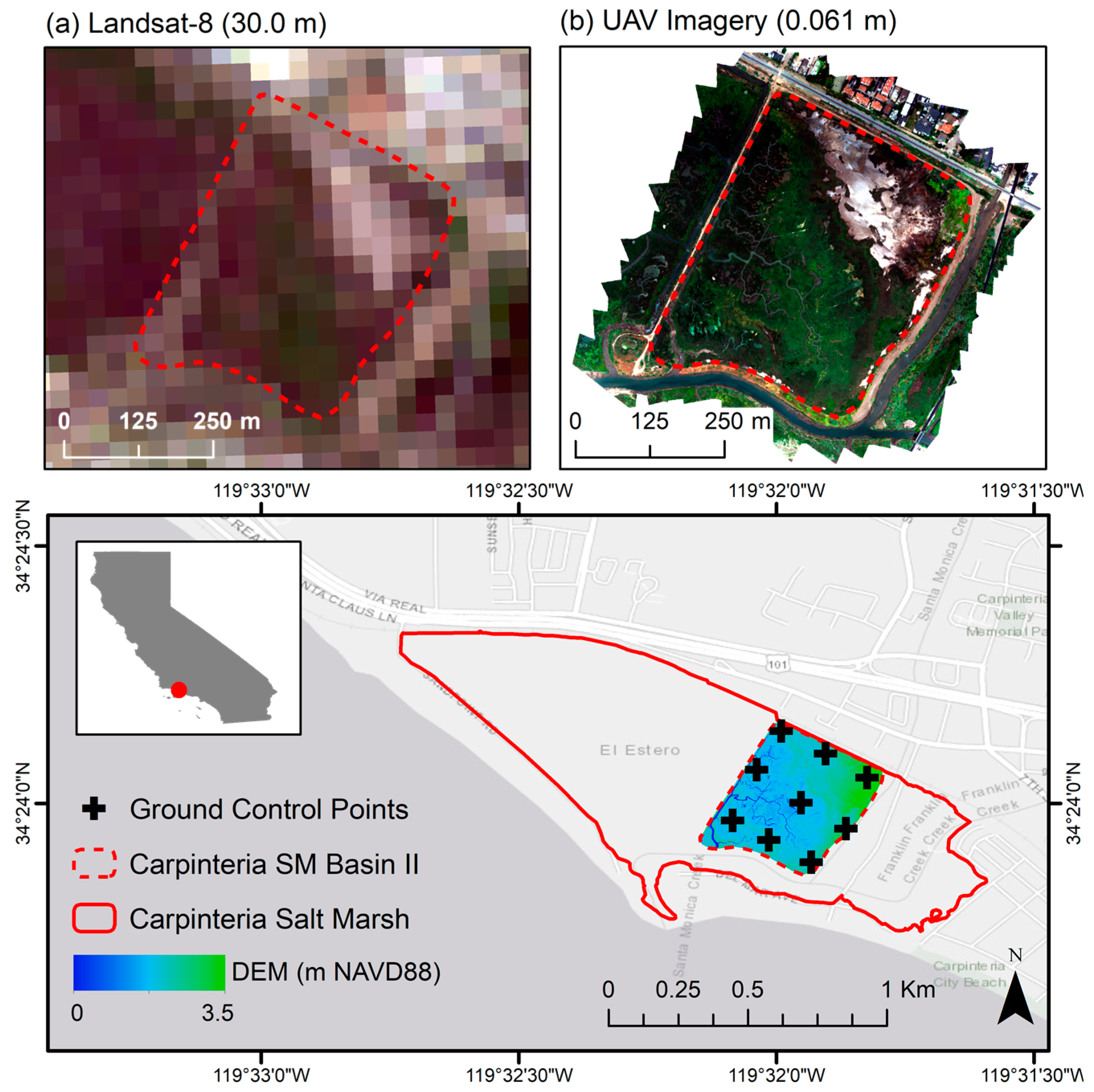
We conducted seasonal UAV surveys and field sampling at the Carpinteria Salt Marsh Reserve (34°24′4.3″N, 119°32′16.4″W), Basin II, in Santa Barbara County, CA, USA between February and November 2018 (Figure 1). This site contains 93 hectares of wetland and channel habitats, in addition to transitional uplands, with relatively shallow elevations grading from −1 m to 3 m above mean sea level. Tidal statistics are characteristic of a perched system with mean sea levels ~0.25 m higher and ~33% reduced tidal range within the marsh relative to the open coast [48]. Climate conditions are Mediterranean temperate with dry, hot summers. Mean temperatures at the site range from 24 °C maximum in August to 6 °C minimum in January, with a mean annual precipitation of 38 cm.
The intertidal plant community consists of annual and perennial herbs and grasses. This site is dominated by Salicornia pacifica (pickleweed), Jaumea carnosa (marsh jaumea), and Distichlis littoralis (shore grass). Other species present include Cuscuta salina (saltmarsh dodder), Frankenia salina (alkali heath), Limonium californicum (marsh rosemary), Distichlis spicata (salt grass), and Suaeda calceoliformis (horned sea blite).
2.2. Field Data Collection
2.2.1. Multispectral UAV Image Data
We conducted field campaigns each season for one year on 23 February 2018 (winter), 24 May 2018 (spring), 19 July 2018 (summer), and 13 November 2018 (fall). Sky conditions on flight days ranged from overcast to clear and tidal levels ranged from 0.24 to 1.29 m NAVD88 (Table S1). We performed UAV surveys using a DJI Matrice 100 quadcopter (DJI, Nanshan, Shenzhen, China). The DJI Matrice 100 is a fully programmable multirotor platform that can be customized with different sensors for specific applications, unlike other off-the-shelf models, like the DJI Phantom. The payload included a Micasense Rededge multispectral camera and a downwelling light sensor (DLS), or irradiance sensor (Micasense, Seattle, WA, USA). However, DLS data were ultimately not included in image processing because it decreased radiometric performance and led to an overestimation of reflectance in the resulting UAV orthomosaic (Figure S1). The Rededge multispectral camera used in this study captures five spectral bands: Blue (475 nm, 20 nm bandwidth), green (560 nm, 20 nm bandwidth), red (668 nm, 10 nm bandwidth), red edge (717 nm, 10 nm bandwidth), and the near-infrared (840 nm, 40 nm bandwidth).
Prior to UAV flight, we deployed ground control place markers (GCPs) with a real-time kinematic global positioning system RTK-GPS to help with georeferencing and photo alignment during image processing (Figure 2). We performed RTK-GPS measurements at GCP centers with an Arrow Gold RTK-GPS with ~3 cm horizontal accuracy and ~5 cm vertical accuracy (EOS Positioning System, Terrebonne, QC, Canada). We also captured images of calibrated panels with known reflectance (Micasense, Seattle, WA, USA) using the Rededge sensor before and after each flight to aid in radiometric conversion.
We planned UAV flights using the Atlas Flight software (Micasense, Seattle, WA, USA). We conducted flights at an altitude of 90 m above ground level, an airspeed of 7 m s−1, and with image overlap (frontlap and sidelap) set to 75%. With these specifications, average flight time per battery set was approximately 30 min, requiring up to 2 flights to cover a 0.35 km2 study area (Table S1).
2.2.2. Vegetation Sampling
We conducted field sampling of salt marsh vegetation during each season along an elevational gradient which captured a representative subset of dominant species at the site (Figure 2, Ground Samples). The elevational gradient ranged from 0 m NAVD88 at the southwest corner of basin II to 3.5 m NAVD88 at the northeast corner of basin II (Figure 1). Along elevational transects, we sampled 0.25-m2 plots (n = 15) placed approximately 10 m apart. We captured plot locations with submeter accuracy using the RTK-GPS. We also measured canopy reflectance with an ASD Handheld 2 Spectrometer (Malvern Panalytical, Malvern, UK). Reflectance spectra were sampled every 1 nm over 325–1075 nm using a 25° field of view foreoptics. We took ten readings at nadir at a height of approximately 50 cm for a 25-cm diameter ground field of view and averaged them together to create a single spectral profile for each plot. Following spectral measurements, we harvested all aboveground biomass above the soil level within the sampling plot. In the laboratory, aboveground biomass samples were massed for wet weight (g), then dried at 50 °C for one week or until constant mass was achieved to obtain dry weight (g).
2.3. Multispectral UAV Image Data Processing
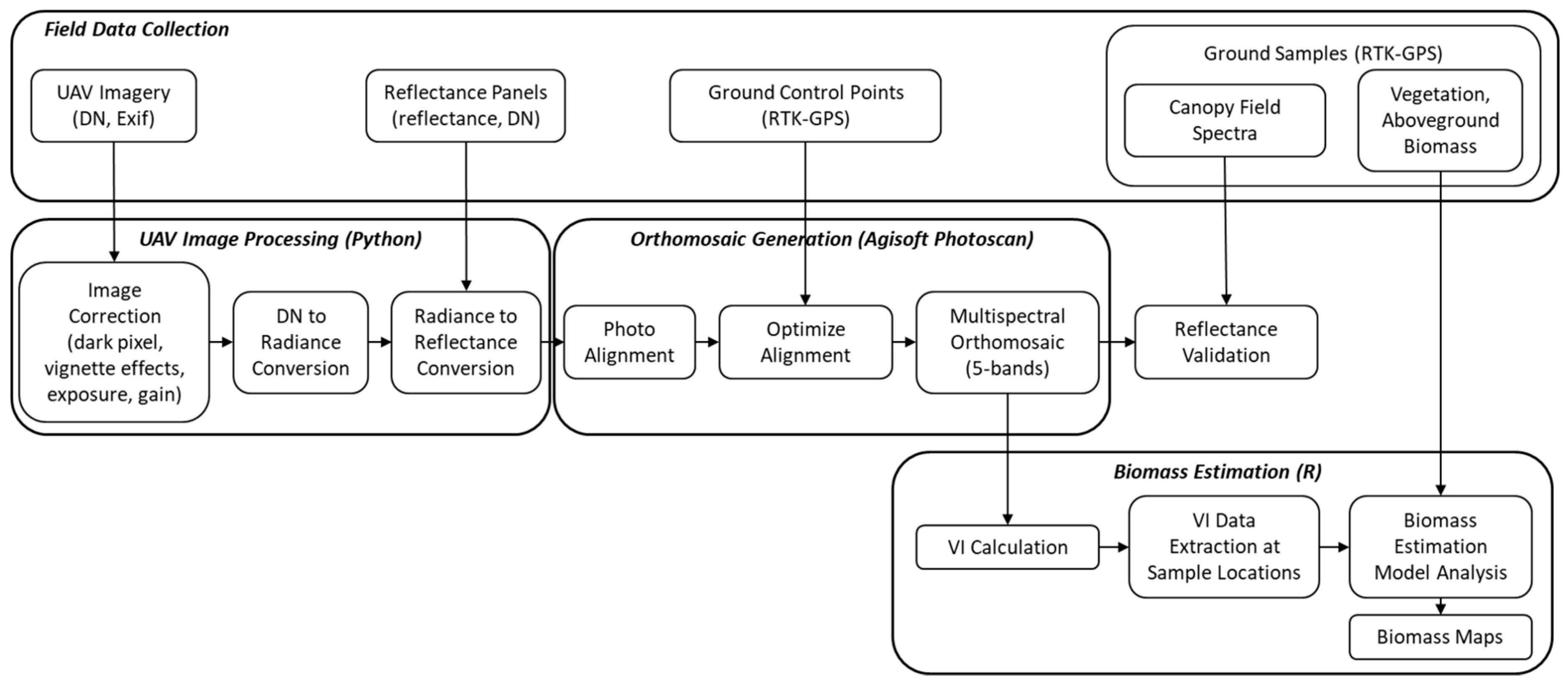
We conducted preprocessing of UAV images to correct images for dark pixels, vignette effects, exposure, and gain (Figure 2). Corrected images were then converted from raw digital number (DN) to radiance and from radiance to reflectance using a radiance-to-reflectance conversion factor calculated by averaging the preflight and postflight calibration panel images. Image correction and radiometric conversion were conducted in Python 3.6 (Python Software Foundation, Amsterdam, the Netherlands) using scripts adapted from Micasense for batch processing [49]. UAV images processed to reflectance were then imported to Agisoft Photoscan Pro v1.4 for orthomosaic generation (Agisoft, St. Petersburg, Russia). During this process, photos were aligned to the highest accuracy setting and optimized using the GCPs with RTK-GPS coordinates. We took additional steps to calibrate image color and white balance to ensure brightness consistency within each band in the resulting orthomosaic. Final processing steps in Photoscan included the creation of a dense point cloud and a digital elevation model (DEM) to facilitate mosaicking. Final orthomosaics for each season covered the Carpinteria Salt Marsh Basin II (Figure 1) at ground resolutions averaging at approximately 6.1 cm pixel−1 (Table S1).
We compared reflectance measured from the UAV imagery to the in situ canopy reflectance measurements to validate data collection and processing. To facilitate comparison, field spectra were first convolved using a weighted average filter to correspond to the bands measured by the Rededge sensor [50]. We processed field spectra in Python 3.6. We extracted reflectance data for each band of the multispectral orthomosaics using the R raster package v2.7. Mean reflectance estimates were extracted for a circular area surrounding each sampling plot, which accounted for quadrat width (25 cm), the horizontal error of both the RTK-GPS (~2.5 cm), and the orthomosaic (4.3–11.9 cm; Table S1). Comparison of UAV and field reflectance for each of the five bands was conducted for pooled seasonal data using simple linear regression in R (R Foundation for Statistical Computing, Vienna, Austria).
2.4. UAV-Based Biomass Estimation
We tested a suite of vegetation indices for their ability to estimate aboveground biomass (Table 1). We selected vegetation indices (VIs) based on the spectral bands present in the Micasense Rededge sensor and to align with common VIs used with multispectral satellite imagery. The UAV-based reflectance estimates corresponding to each sampling plot were then used to calculate average VI for each plot. We compared plot aboveground biomass to VIs for pooled seasonal data, as well as separately for each season, using simple linear regression from the R stats package v3.4.2. Linear regression analysis was selected because data derived from the orthomosaics did not exhibit pixel saturation.
We selected the vegetation index with the highest performing biomass estimation model to create biomass maps for each season. We chose a single annual model based on the seasonally pooled data to allow for comparison across seasons. To create biomass maps, first, we created VI maps from the 5-band multispectral orthomosaics using raster band math functions in R. Then, we applied the biomass estimation model to the VI maps to create biomass maps. Additional raster processing included the masking of water and resampling so that resulting biomass maps conform to a 1-m pixel resolution. Water masks were created using a supervised classification in ENVI (Harris Geospatial Solutions, Boulder, CO, USA). All raster processing was conducted in R.
Further investigation of annual versus seasonal models was performed for the highest performing VI. We used a partial F-test to compare the reduced model (pooled seasonal data) and the full model (including season as a predictor variable). All statistical analyses were performed in R.
2.5. Spatial and Temporal Analysis of Biomass
We used the UAV-derived maps of biomass to estimate the mean aboveground biomass density and total aboveground biomass for the site in each season. We tested seasonal differences using a two-way ANOVA. Data were square root-transformed to meet assumptions of normality and homogeneity of variances as needed. Biomass maps were also compared to 1-m2 resolution digital elevation models (DEMs) available from the NOAA-CA Coastal Conservancy Coastal LiDAR project 2009–2013. Biomass and elevation data were extracted for each pixel along an elevational gradient from the SW corner to the NE corner of Basin II (Figure 1). The correlation of biomass and elevation was tested using a parabolic linear regression in R.
3. Results
3.1. Spectral Reflectance Validation
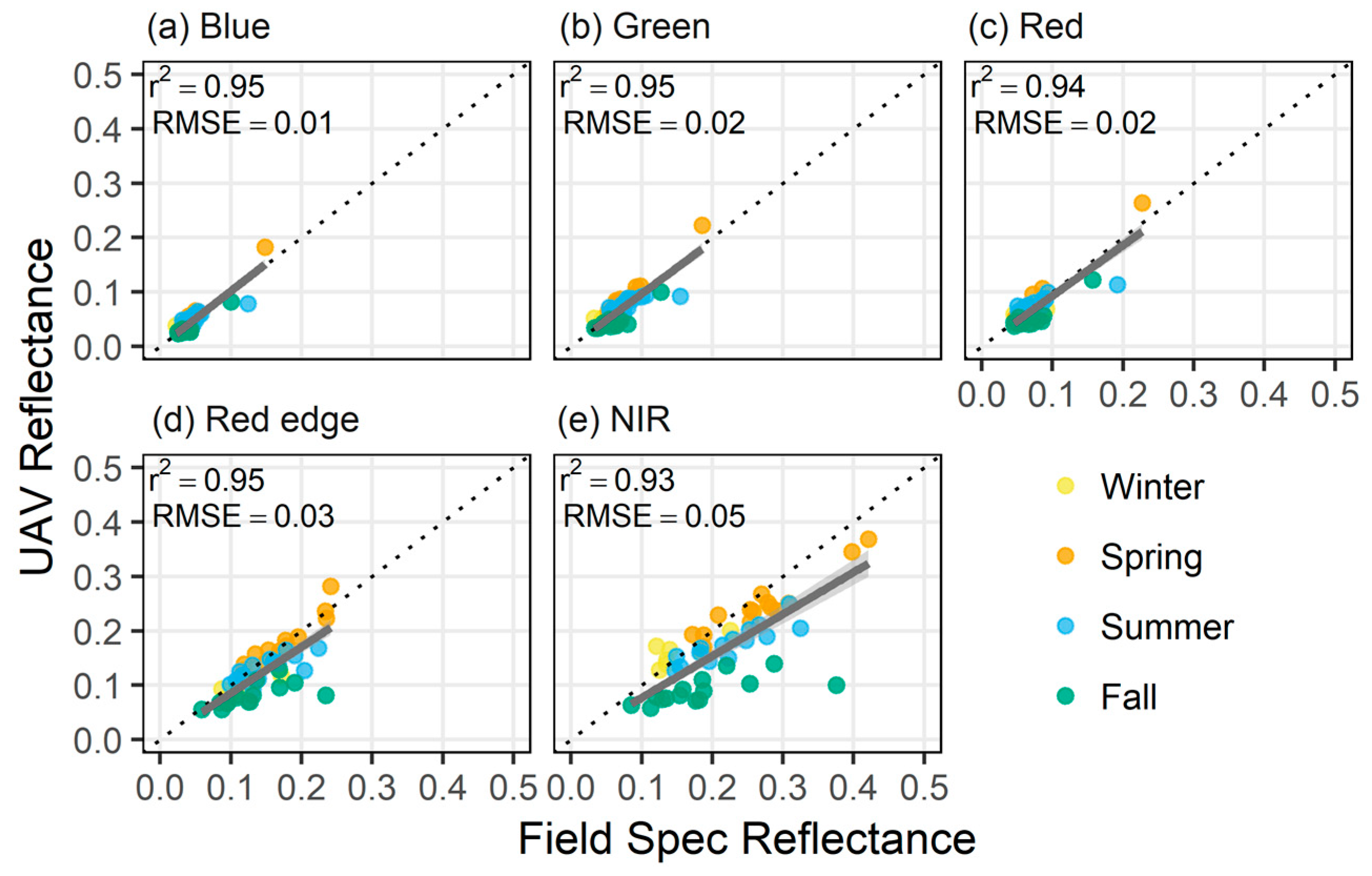
Comparison of field and UAV-based reflectance measurements pooled for all seasons indicated a strong 1:1 correlation (r2 ≥ 0.94) with root mean square error (RMSE) less than 0.02 for all visible bands (Figure 3). The rededge (RE) and near-infrared (NIR) bands exhibited more variability at higher reflectance values. Overall, reflectance estimated with the UAV imagery and the observed reflectance in the field were well-correlated in the RE and NIR (r2 ≥ 0.93), with RMSE’s less than 0.05. Linear regression models for each band were found to be statistically significant (p < 0.005).
3.2. Biomass Estimation Models
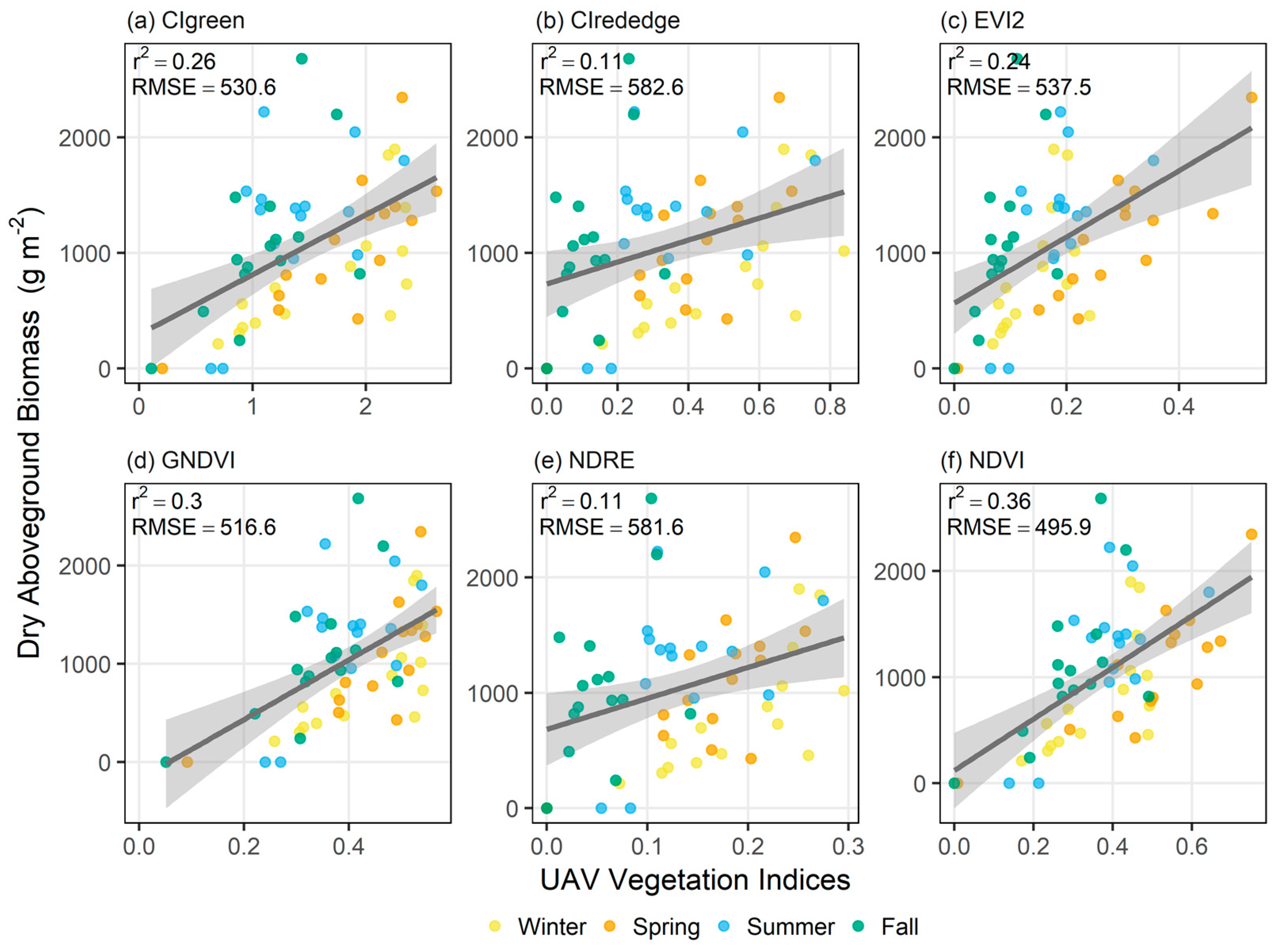
The vegetation indices exhibited variable performance in estimating aboveground biomass (Figure 4, Table 2). Of the vegetation indices, NDVI had the strongest linear correlation to dry aboveground biomass for pooled seasonal data (r2 = 0.36, RMSE = 495.9 g m−2, p < 0.005; Table 2), and for each season when seasonal data was analyzed individually. Live aboveground biomass was also best predicted by NDVI compared to the other VIs (Table S2).
Further analysis of the NDVI-based biomass estimation model reveals that season is a significant predictor in estimating aboveground biomass (partial F-test, F = 6.13, p < 0.001). NDVI-aboveground biomass models for the individual seasons exhibited variable success in predicting biomass (Table 3). Although linear models were significant for all seasons, spring had the best performing model (r2 = 0.67, RMSE = 344.3 g m−2). For live aboveground biomass, the spring biomass estimation model also outperformed all other seasons (Table S3).
3.3. Spatial and Temporal Patterns in Aboveground Biomass
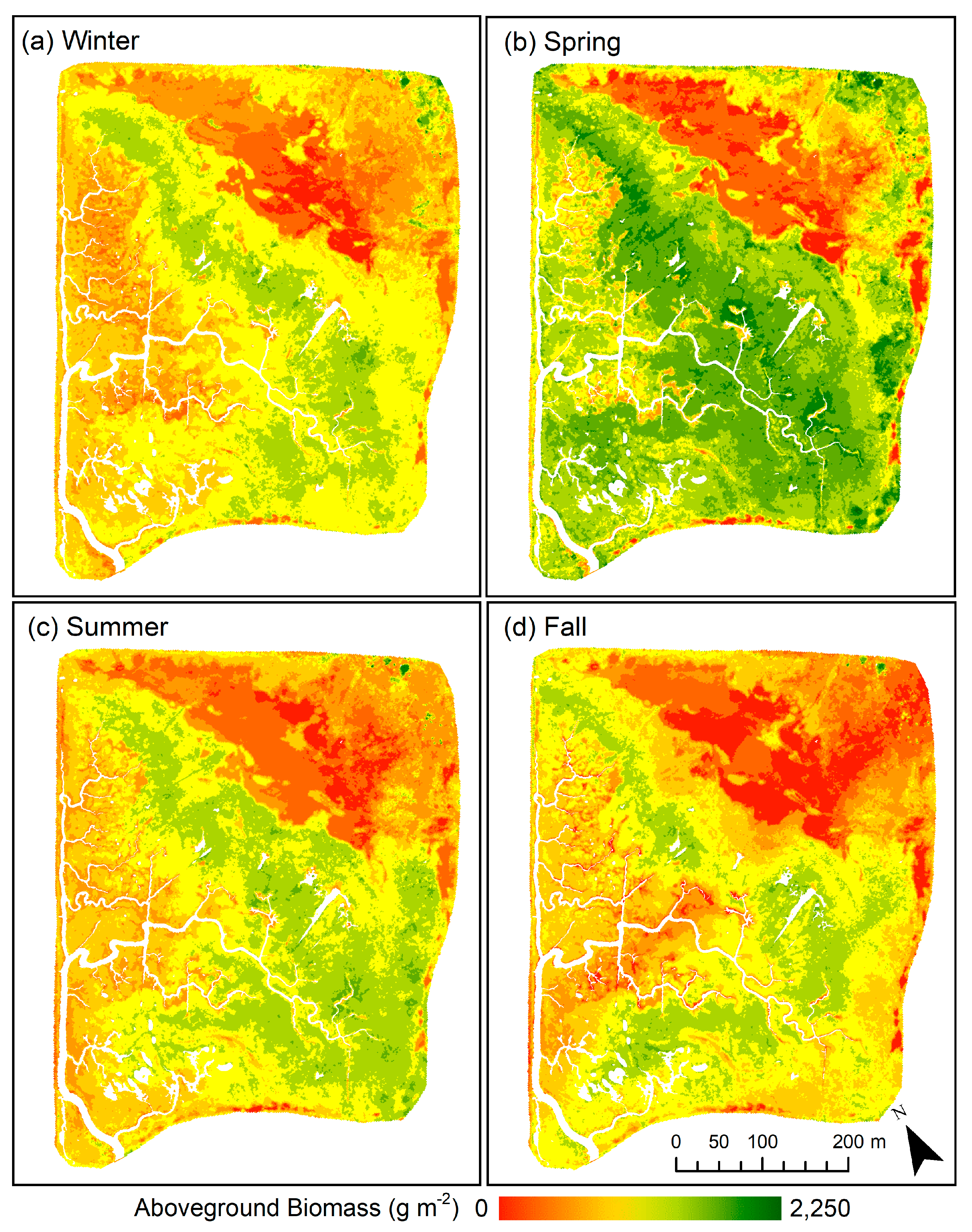
The annual NDVI-based biomass estimation model (Equation (1)) was selected to create comparable biomass maps for Basin II of the Carpinteria Salt Marsh Reserve for each season (Figure 5). Visual comparison of seasonal biomass maps reveals peak biomass indicative of salt marsh vegetation “green-up” occurring in spring. Analysis of pixel data for each biomass map also indicates an increase in average aboveground biomass in spring, which was estimated to be 1222.9 ± 435.7 g m−2 (Table 4). This was 295.3 g m−2 higher than the average aboveground biomass estimated for the site in winter, summer, and fall. Similarly, total site biomass in Carpinteria Salt Marsh Basin II was 204.7 Mg in spring, approximately 49.3 Mg higher than total site biomass estimated for winter, summer, and fall.
AGB = 2428.2 × NDVI + 120.1
The seasonal patterns suggested by the biomass maps were supported by field observations and analysis of field biomass (Table 4). Spring and summer exhibited higher dry and wet aboveground biomass compared to that of fall and winter. Unlike the UAV-derived biomass estimates, field data suggests peak plot biomass occurred in summer, which may be indicative of ongoing biomass accumulation from spring to summer coinciding with slight declines in vegetation greenness. However, only wet aboveground biomass was found to be significantly different among seasons (p < 0.001). Dry aboveground was not significantly different across seasons (p = 0.27).
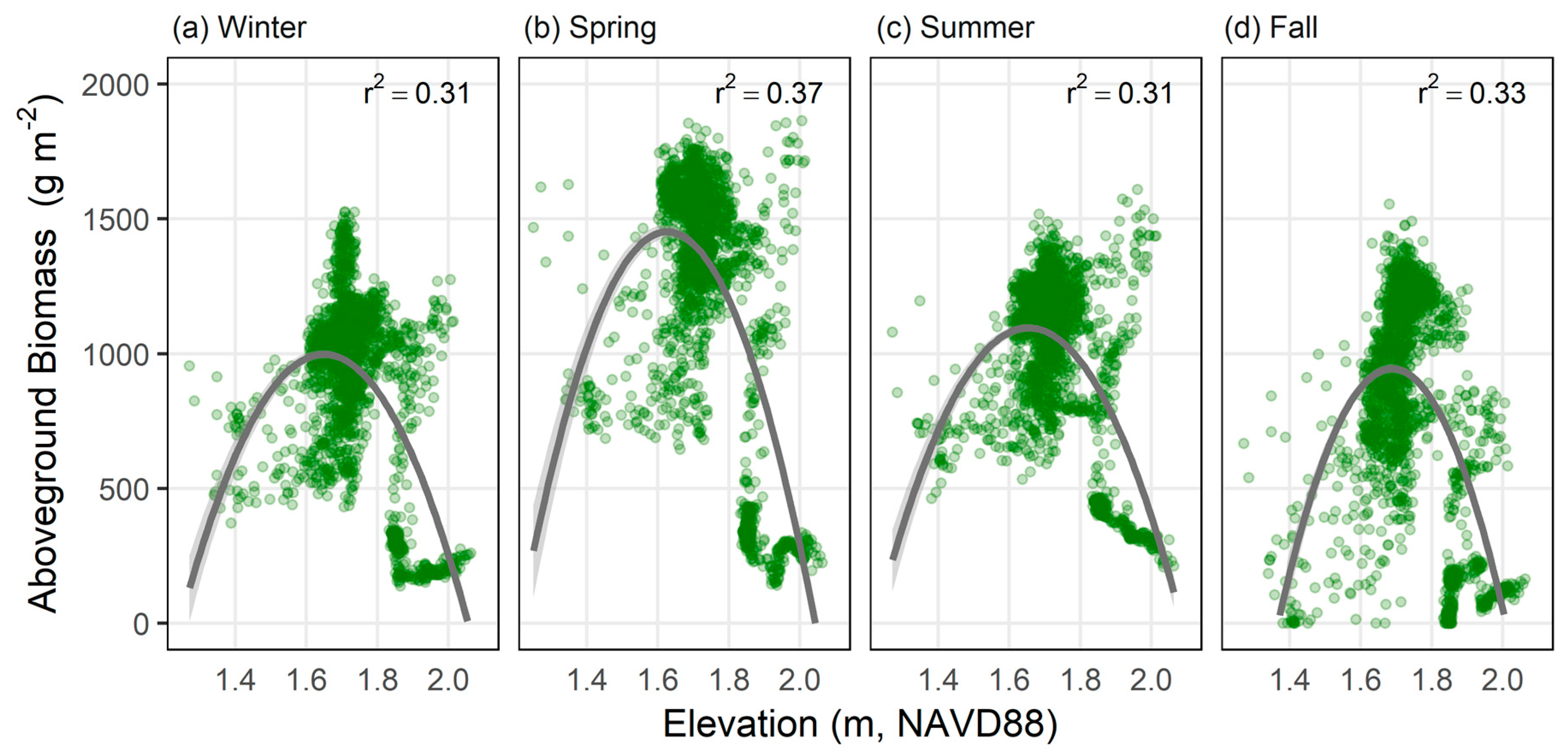
UAV-derived estimates of biomass were compared to elevation for a subset of marsh area along an elevational gradient (Figure 6). For all seasons, peak biomass estimates occurred at elevations of 1.6 to 1.8 m. Maximum biomass occurred in spring with averages nearing 1500 g m−2, which was, on average, approximately 500 g m−2 higher than the other seasons.
4. Discussion
This study demonstrates the potential for mapping aboveground biomass in coastal wetlands using high-resolution multispectral UAV imagery. By combining a UAV approach and field surveys over the course of an annual growing cycle, we were able to develop biomass estimation models based on NDVI, a commonly used proxy for vegetation health and productivity. We found a strong relationship between NDVI and biomass during the spring, which is typically the season of peak greenness. The submeter ground resolution attainable with UAVs was beneficial for investigating fine-scale spatial changes in wetland biomass. UAVs also offer high flexibility in the timing of imagery collection, which would be beneficial for a number of time-sensitive ecological applications. Overall, the multi-temporal, multispectral imagery derived from UAVs can help reveal spatio-temporal variability at resolutions superior to traditional remote sensing approaches.
Our findings reveal the high spatial and temporal variability of aboveground biomass in the Carpinteria Salt Marsh Reserve. The biomass maps created for this site indicate pronounced seasonal variability in vegetation health and biomass (Figure 5). This pattern is characteristic of southern California coastal marshes where green-up of vegetation generally occurs in spring following the rainy season with biomass then peaking at the end of summer, followed by senescence [57,58]. Our biomass maps capture spring green-up but indicate an overall reduction in green vegetation and aboveground biomass in summer (Table 4). This seasonal, site-wide response may be explained by spatial variation in vegetation productivity occurring within the marsh due to environmental stress along elevational gradients (Figure 6). High soil salinity is a major limiting factor for wetland plant growth in southern California [57], and soil salinity has been shown to vary spatially with elevation and tidal inundation [59]. While productivity at lower elevations is generally limited by inundation [60,61,62], higher elevations are prone to increased soil salinities due to reduced tidal flushing, minimal freshwater inputs and high rates of evapotranspiration in hot, dry summer months [63,64]. Previous work in the Carpinteria salt marsh indicates reduced tidal exchange within the marsh, with higher elevations receiving as little as 5% of the inundation experienced at lower elevations [48]. This case site exemplifies how the high spatial resolutions and flexible temporal sampling frequency provided by UAVs can aid in investigating ecologically meaningful patterns and processes occurring within salt marshes.
However, there is uncertainty associated with the remotely sensed estimates of aboveground biomass that can be attributed to several sources of error caused by the coastal environment, as well as data collection and processing techniques [13]. Environmental factors, such as sky conditions and tidal stage at the time of UAV flight can contribute to radiometric variability. Sky conditions, namely the presence of clouds, have been shown to influence the radiometric correction and resulting homogeneity of the UAV orthophotos [47]. We conducted our UAV flights over the course of a year under varying sky conditions. Environmental conditions during field campaigns contribute to radiometric variability, as evidenced by seasonal differences in the correlation among UAV and in situ measures of reflectance in the rededge and near-infrared wavelengths (Figure 3). This is shown by data collected in the fall, where variability in incoming irradiance associated with partly cloudy conditions led to an underestimation of reflectance by the UAV compared to the canopy reflectance measured in situ. Where possible, UAV imagery should be collected under constant sky conditions as close to solar noon as possible [47] in accordance with other logistical, regulatory, and weather constraints. In addition, the use of a downwelling light sensor, or irradiance sensor, may improve issues arising from variable light conditions; however, in this study, tests including irradiance data during image processing resulted in overestimation of reflectance in UAV imagery, thus, were excluded (Figure S1). Finally, sensor noise may also present a significant source of radiometric variability and should be considered when selecting and designing UAV payloads.
The presence of water also poses significant complications to estimating biomass in coastal wetlands using remote sensing approaches. Water inundation dampens the reflectance occurring in the near-infrared wavelengths [26] and so will affect vegetation indices such as NDVI. The depth of inundation, vegetation structure, and underlying soils can ultimately interfere with the relationship between reflectance and standing biomass [16]. This concern has been demonstrated in long-term time series analyses of wetlands, where high NDVI outliers are more likely to reflect real changes in vegetation, but low outliers are likely to be artifacts of clouds or inundation [65]. The use of NDVI in this study as the foundation for biomass estimation models, therefore, comes with similar concerns. Due to sampling constraints and our desire to conduct UAV surveys as close to noon as possible, tidal levels varied across our survey dates. As a result, tidal inundation could lead to underestimation of NDVI and affect the relationship between NDVI and biomass. To reduce errors associated with inundation, water was masked for each season using a standardized classification. However, spatial analysis of the final biomass maps reveals potential issues caused by the presence of underlying water in vegetation canopies. In particular, the fall campaign was conducted with tidal levels over two times higher than the other seasons (Table S1), which may have resulted in underestimation of biomass, especially in pixels coinciding with lower elevations where tidal inundation is more probable (Figure 6). However, one of the benefits of UAV imagery is that the user has control over the timing of image acquisition. Therefore, field campaigns can be planned so that multi-temporal images are collected at similar tidal stages.
Vegetation phenology likely also impacted our UAV based estimates of biomass. The NDVI-based aboveground biomass model was significantly improved when season was considered as an additional predictor variable, meaning that season plays a significant role in predicting aboveground biomass. Further analysis of biomass estimation models for the individual seasons shows that, although biomass estimation models for each season were significant (Table 3), spring presents the strongest model for estimating biomass. One key reason for this finding relates to the relationship between greenness and biomass. NDVI is essentially a measure of vegetation greenness, therefore, it serves best as a predictor of live, green biomass, which is typically produced during the growing season beginning in spring [57]. This is also evident in NDVI-based biomass estimation models developed for live, or wet, vegetation (Table S2, Table S3). Following the summer and fall dry season, salt marsh perennial and annual plants have either senesced or died, often resulting in higher levels of non-photosynthetic vegetation (NPV). During summer, fall, and winter, poor correlation can be expected between NDVI and biomass due to a lack of green biomass, given the environmental stressors and natural phenological cycles at play in these Mediterranean coastal wetland systems. As a result, we recommend that studies examining interannual variability in marsh biomass in this region should conduct multispectral UAV surveys during the spring. These findings also have implications for satellite-based assessments, where peak biomass may be the most informative biomass estimate for detecting long term changes associated with environmental variability [8]. This has been shown in other satellite-based assessments. For example, [21] found a strong correlation (r2 = 0.70) between NDVI and peak biomass in Spartina dominated salt marshes on the coast of Georgia.
Further improvements to biomass estimation using UAVs in coastal wetlands can be achieved by more accurately capturing NPV. Fortunately, the ground resolutions provided by UAVs offer a number of advantages for mapping and monitoring coastal wetlands. For instance, the increased spatial resolution of ground pixels leads to a decrease in the number of mixed pixels, which might contain both green vegetation and NPV. The spectral response of an unmixed pixel will be more representative of a single vegetation cover type, whereas mixed pixels constitute a combination of spectral responses from multiple, often disparate, cover types. For example, spectral signatures can vary among herbaceous or woody vegetation types due to the biochemical and biophysical properties of the vegetation [66,67] and therefore, may be more easily differentiated at finer resolutions. Increased spatial resolution has a proven advantage in delineating vegetation classes and estimating percent cover in salt marshes [42,68] and mangroves [39] using multispectral imagery. Additionally, increased spectral resolution can also aid in the differentiation of cover types like live vegetation and NPV. Hyperspectral imagery has demonstrated an advantage over broad-band multispectral imagery with improved accuracies in differentiating vegetation types and species [13]. Gains in both spatial and spectral resolution can increase sensitivity to variations in reflectance or vegetation indices and ultimately improve the separability of different vegetation types.
High-resolution information on vegetation height and structure is another important component that could improve biomass estimation in coastal wetlands. Vegetation height and structure are typically measured remotely using active sensors such as LiDAR and RADAR [69]. These types of sensors can be placed on UAVs, but they are relatively expensive as compared to multispectral optical sensors. As UAV and sensor technology advances, the inclusion of active sensors to UAV payloads will become more feasible [27,46]. However, passive optical sensors onboard UAVs also have the potential to provide structural information using photogrammetric methods in coastal wetlands [40]. These approaches have been successfully applied in olive orchards, temperate deciduous forests, and mangrove forests [43,70,71]. However, mapping vegetation height using photogrammetry is challenging in dense coastal wetlands as it is difficult to obtain sufficient numbers of ground points required to calculate vegetation height. For example, errors of up to 80% have been documented in elevation models created for dense cordgrass habitats [41].
5. Conclusions
Here, we demonstrate that UAVs can aid our understanding of the spatial and temporal patterns in salt marsh biomass and productivity. Improved understanding of how productivity and biomass change over seasonal, annual, and decadal time scales is especially valuable, because this could indicate deviations from normal patterns of coastal wetland health. But, in order to detect ecologically relevant changes, remote sensing methods must capture both press and pulse disturbances that operate at vastly different temporal scales. In particular, discrete pulse disturbances often require flexibility and rapid deployment to time sampling efforts appropriately in order to capture the impacts to coastal wetlands. Impacts to biomass, productivity, and wetland health could serve as harbingers of future climate change impacts and could help establish thresholds of resilience to climate change drivers. Assessment of changes to biomass and productivity also highlight the potential for high-resolution insights into climate-related threats to ecosystem services, like carbon storage, that are provided by these valuable coastal habitats.
The benefits of UAVs for ecological applications in coastal wetlands are numerous due to their high operational flexibility and relatively low cost. This is a key advantage over traditional aerial and satellite remote sensing. Furthermore, UAVs are a valuable addition to traditional ecological fieldwork, which can often be time- and resource-intensive and costly and may limit the scope of study to relatively small areas and periods of time. Therefore, UAVs may be a complementary approach to fill critical spatial and temporal gaps inherent to both field work and other remotely sensed data. Integrating contextual field data, high-accuracy GPS, and both UAV and satellite remote sensing approaches can improve our ability to estimate biomass and productivity over time. Overall, remotely sensed data with high spatial and temporal resolutions could provide a more synoptic understanding of coastal wetland ecology and an invaluable view of ecological patterns and processes.
Supplementary Materials
The following are available online at https://0-www-mdpi-com.brum.beds.ac.uk/2072-4292/11/5/540/s1, Figure S1: Radiomatric performance of UAV orthomosaic with and without the inclusion of downwelling light sensor (DLS) data in image processing, Table S1: Site conditions and flight data for seasonal field surveys, Table S2: Live aboveground biomass estimation equations for vegetation indices, Table S3: Seasonal NDVI-live aboveground biomass estimation equations.
Author Contributions
Conceptualization, C.L.D. and K.C.C.; methodology, C.L.D. and K.C.C.; software, C.L.D. and K.C.C.; validation, C.L.D. and K.C.C.; formal analysis, C.L.D.; investigation, C.L.D. and K.C.C.; resources, K.C.C.; data curation, C.L.D.; writing—original draft preparation, C.L.D. and K.C.C.; writing—review and editing, C.L.D. and K.C.C.; visualization, C.L.D.; supervision, K.C.C.; project administration, K.C.C.; funding acquisition, K.C.C.
Funding
Funding for this work was provided by the NASA New Investigator Program (NNX16AN04G). Cheryl Doughty was also supported by a Graduate Research Mentorship and Summer Graduate Research Mentorship at the University of California, Los Angeles.
Acknowledgments
We would like to thank the University of California Natural Reserve System, UCSB Carpinteria Salt Marsh Reserve and site director, Andrew Brookes, for providing access to the field site. Special thanks to Daniel Jensen, Kate Cavanaugh, and Jessica Fayne for their help conducting field work and Amanda Wagner, Nickie Cammis, Marisol Hernandez-Cira, and Jessica Kurylo for laboratory access. Lastly, we thank the editors and the anonymous reviewers whose suggestions have greatly improved the quality of the manuscript.
Conflicts of Interest
The authors declare no conflict of interest.
References
- Day, J.W.; Christian, R.R.; Boesch, D.M.; Yáñez-Arancibia, A.; Morris, J.; Twilley, R.R.; Naylor, L.; Schaffner, L.; Stevenson, C. Consequences of climate change on the ecogeomorphology of coastal wetlands. Estuaries Coasts 2008, 31, 477–491. [Google Scholar] [CrossRef]
- Morris, J.T.; Sundareshwar, P.V.; Nietch, C.T.; Kjerfve, B.B.; Cahoon, D.R. Responses of coastal wetlands to rising sea level. Ecology 2002, 83, 2869–2877. [Google Scholar] [CrossRef]
- Pennings, S.C.; Grant, M.B.; Bertness, M.D. Plant zonation in low-latitude salt marshes: Disentangling the roles of flooding, salinity and competition. J. Ecol. 2005, 93, 159–167. [Google Scholar] [CrossRef]
- Kirwan, M.L.; Guntenspergen, G.R. Response of plant productivity to experimental flooding in a stable and a submerging marsh. Ecosystems 2015, 18, 903–913. [Google Scholar] [CrossRef]
- Kirwan, M.L.; Megonigal, J.P. Tidal wetland stability in the face of human impacts and sea-level rise. Nature 2013, 504, 53–60. [Google Scholar] [CrossRef] [PubMed]
- Scavia, D.; Field, J.C.; Boesch, D.F.; Buddemeier, R.W.; Cayan, D.R.; Fogarty, M.; Harwell, M.A.; Howarth, R.W.; Reed, D.J.; Royer, T.C.; et al. Climate Change Impacts on U.S. Coastal and Marine Ecosystems. Estuaries 2002, 25, 149–164. [Google Scholar] [CrossRef]
- Osland, M.J.; Enwright, N.M.; Day, R.H.; Gabler, C.A.; Stagg, C.L.; Grace, J.B. Beyond just sea-level rise: Considering macroclimatic drivers within coastal wetland vulnerability assessments to climate change. Glob. Chang. Biol. 2016. [Google Scholar] [CrossRef] [PubMed]
- Buffington, K.J.; Dugger, B.D.; Thorne, K.M. Climate-related variation in plant peak biomass and growth phenology across Pacific Northwest tidal marshes. Estuar. Coast. Shelf Sci. 2018, 202, 212–221. [Google Scholar] [CrossRef]
- Janousek, C.N.; Buffington, K.J.; Thorne, K.M.; Guntenspergen, G.R.; Takekawa, J.Y.; Dugger, B.D. Potential effects of sea-level rise on plant productivity: Species-specific responses in northeast Pacific tidal marshes. Mar. Ecol. Prog. Ser. 2016, 548, 111–125. [Google Scholar] [CrossRef]
- Goodman, A.C.; Thorne, K.M.; Buffington, K.J.; Freeman, C.M.; Janousek, C.N. El Niño Increases High-Tide Flooding in Tidal Wetlands Along the U.S. Pacific Coast. J. Geophys. Res. Biogeosci. 2018, 123, 3162–3177. [Google Scholar] [CrossRef]
- Klemas, V. Remote sensing of coastal wetland biomass: An overview. J. Coast. Res. 2013, 290, 1016–1028. [Google Scholar] [CrossRef]
- Klemas, V.V. Remote Sensing of Coastal Ecosystems and Environments. Remote Sens. Model. 2009, 8. [Google Scholar] [CrossRef]
- Adam, E.; Mutanga, O.; Rugege, D. Multispectral and hyperspectral remote sensing for identification and mapping of wetland vegetation: A review. Wetl. Ecol. Manag. 2010, 18, 281–296. [Google Scholar] [CrossRef]
- Ozesmi, S.L.; Bauer, M.E. Satellite remote sensing of wetlands. Wetl. Ecol. Manag. 2002, 10, 381–402. [Google Scholar] [CrossRef]
- Mishra, D.R.; Ghosh, S. Using Moderate-Resolution Satellite Sensors for Monitoring the Biophysical Parameters and Phenology of Tidal Marshes. In Remote Sensing of Wetlands: Applications and Advances; CRC Press: Boca Raton, FL, USA, 2015; pp. 300–331. [Google Scholar]
- Byrd, K.B.; O’Connell, J.L.; Di Tommaso, S.; Kelly, M. Evaluation of sensor types and environmental controls on mapping biomass of coastal marsh emergent vegetation. Remote Sens. Environ. 2014, 149, 166–180. [Google Scholar] [CrossRef]
- Mutanga, O.; Skidmore, A.K. Narrow band vegetation indices overcome the saturation problem in biomass estimation. Int. J. Remote Sens. 2004, 25, 3999–4014. [Google Scholar] [CrossRef]
- Xue, J.; Su, B. Significant remote sensing vegetation indices: A review of developments and applications. J. Sens. 2017, 2017, 1–17. [Google Scholar] [CrossRef]
- Zhang, M.; Ustin, S.L.; Rejmankova, E.; Sanderson, E.W. Monitoring Pacific Coast Salt Marshes Using Remote Sensing. Ecol. Appl. 1997, 7, 1039–1053. [Google Scholar] [CrossRef]
- Mutanga, O.; Adam, E.; Cho, M.A. High density biomass estimation for wetland vegetation using worldview-2 imagery and random forest regression algorithm. Int. J. Appl. Earth Obs. Geoinf. 2012, 18, 399–406. [Google Scholar] [CrossRef]
- O’Donnell, J.P.R.; Schalles, J.F. Examination of abiotic drivers and their influence on Spartina alterniflora biomass over a twenty-eight year period using Landsat 5 TM satellite imagery of the Central Georgia Coast. Remote Sens. 2016, 8, 477. [Google Scholar] [CrossRef]
- Gallant, A.L. The challenges of remote monitoring of wetlands. Remote Sens. 2015, 7, 10938–10950. [Google Scholar] [CrossRef]
- Shanmugam, P. Remote Sensing of the Coastal Ecosystems. J. Geophys. Remote Sens. 2013, S2, e001. [Google Scholar] [CrossRef]
- Zomer, R.J.; Trabucco, A.; Ustin, S.L. Building spectral libraries for wetlands land cover classification and hyperspectral remote sensing. J. Environ. Manag. 2009, 90, 2170–2177. [Google Scholar] [CrossRef] [PubMed]
- Schmidt, K.S.; Skidmore, A.K. Spectral discrimination of vegetation types in a coastal wetland. Remote Sens. Environ. 2003, 85, 92–108. [Google Scholar] [CrossRef]
- Kearney, M.S.; Stutzer, D.; Turpie, K.; Stevenson, J.C. The Effects of Tidal Inundation on the Reflectance Characteristics of Coastal Marsh Vegetation. J. Coast. Res. 2009, 256, 1177–1186. [Google Scholar] [CrossRef]
- Whitehead, K.; Hugenholtz, C.H.; Myshak, S.; Brown, O.; LeClair, A.; Tamminga, A.; Barchyn, T.E.; Moorman, B.; Eaton, B. Remote sensing of the environment with small unmanned aircraft systems (UASs), part 1: A review of progress and challenges. J. Unmanned Veh. Syst. 2014, 2, 86–102. [Google Scholar] [CrossRef]
- Klemas, V.V. Coastal and Environmental Remote Sensing from Unmanned Aerial Vehicles: An Overview. J. Coast. Res. 2015, 315, 1260–1267. [Google Scholar] [CrossRef] [Green Version]
- Manfreda, S.; Mccabe, M.; Miller, P.; Lucas, R.; Pajuelo, V.M.; Mallinis, G.; Ben Dor, E.; Helman, D.; Estes, L.; Ciraolo, G.; et al. On the Use of Unmanned Aerial Systems for Environmental Monitoring. Remote Sens. 2018, 10, 641. [Google Scholar] [CrossRef]
- Vincent, J.B.; Weden, L.K.; Ditmer, M.A. Barriers to adding UAVs to the ecologist’s toolbox. Front. Ecol. Environ. 2014, 13, 73–74. [Google Scholar] [CrossRef]
- Hugenholtz, C. Small unmanned aircraft systems for remote sensing and earth science research. Eos 2012, 93, 24–25. [Google Scholar] [CrossRef]
- Turner, I.L.; Harley, M.D.; Drummond, C.D. UAVs for coastal surveying. Coast. Eng. 2016, 114, 19–24. [Google Scholar] [CrossRef]
- Hugenholtz, C.H.; Whitehead, K.; Brown, O.W.; Barchyn, T.E.; Moorman, B.J.; LeClair, A.; Riddell, K.; Hamilton, T. Geomorphological mapping with a small unmanned aircraft system (sUAS): Feature detection and accuracy assessment of a photogrammetrically-derived digital terrain model. Geomorphology 2013, 194, 16–24. [Google Scholar] [CrossRef] [Green Version]
- Delacourt, C.; Allemand, P.; Jaud, M.; Grandjean, P.; Deschamps, A.; Ammann, J.; Cuq, V. DRELIO: An Unmanned Helicopter for Imaging Coastal Areas. J. Coast. Res. 2009, 56, 1489–1493. [Google Scholar]
- Pereira, E.; Bencatel, R.; Correia, J.; Felix, L.; Goncalves, G.; Morgado, J.; Sousa, J. Unmanned air vehicles for coastal and environmental research. J. Coast. Res. 2009, 56, 1557–1561. [Google Scholar]
- Chong, A.K. HD aerial video for coastal zone ecological mapping. In Proceedings of the SIRC 2007—19th Annual Colloquium of the Spatial Information Research Center, University of Otago, Dunedin, New Zealand, 6–7 December 2007. [Google Scholar]
- Jensen, A.M.; Hardy, T.; McKee, M.; Chen, Y. Using a multispectral autonomous unmanned aerial remote sensing platform (AggieAir) for riparian and wetlands applications. Int. Geosci. Remote Sens. Symp. 2011, 3413–3416. [Google Scholar] [CrossRef]
- Samiappan, S.; Turnage, G.; Hathcock, L.A.; Moorhead, R. Mapping of invasive phragmites (common reed) in Gulf of Mexico coastal wetlands using multispectral imagery and small unmanned aerial systems. Int. J. Remote Sens. 2016, 38, 1–22. [Google Scholar] [CrossRef]
- Ruwaimana, M.; Satyanarayana, B.; Otero, V.; Muslim, A.M.; Muhammad Syafiq, A.; Ibrahim, S.; Raymaekers, D.; Koedam, N.; Dahdouh-Guebas, F. The advantages of using drones over space-borne imagery in the mapping of mangrove forests. PLoS ONE 2018, 13, 1–22. [Google Scholar] [CrossRef] [PubMed]
- Kalacska, M.; Chmura, G.L.; Lucanus, O.; Bérubé, D.; Arroyo-Mora, J.P. Structure from motion will revolutionize analyses of tidal wetland landscapes. Remote Sens. Environ. 2017, 199, 14–24. [Google Scholar] [CrossRef]
- Meng, X.; Shang, N.; Zhang, X.; Li, C.; Zhao, K.; Qiu, X.; Weeks, E. Photogrammetric UAV mapping of terrain under dense coastal vegetation: An object-oriented classification ensemble algorithm for classification and terrain correction. Remote Sens. 2017, 9, 1187. [Google Scholar] [CrossRef]
- Zhou, Z.; Yang, Y.; Chen, B. Estimating Spartina alterniflora fractional vegetation cover and aboveground biomass in a coastal wetland using SPOT6 satellite and UAV data. Aquat. Bot. 2018, 144, 38–45. [Google Scholar] [CrossRef]
- Otero, V.; Van De Kerchove, R.; Satyanarayana, B.; Martínez-Espinosa, C.; Fisol, M.A.; Ibrahim, M.R.; Sulong, I.; Mohd-Lokman, H.; Lucas, R.; Dahdouh-Guebas, F. Managing mangrove forests from the sky: Forest inventory using field data and Unmanned Aerial Vehicle (UAV) imagery in the Matang Mangrove Forest Reserve, peninsular Malaysia. For. Ecol. Manage. 2018, 411, 35–45. [Google Scholar] [CrossRef]
- Sugiura, R.; Noguchi, N.; Ishii, K. Remote-sensing Technology for Vegetation Monitoring using an Unmanned Helicopter. Biosyst. Eng. 2005, 90, 369–379. [Google Scholar] [CrossRef]
- Berni, J.A.J.; Member, S.; Zarco-tejada, P.J.; Suárez, L.; Fereres, E. Thermal and Narrowband Multispectral Remote Sensing for Vegetation Monitoring From an Unmanned Aerial Vehicle. IEEE Trans. Geosci. Remote Sens. 2009, 47, 722–738. [Google Scholar] [CrossRef] [Green Version]
- Whitehead, K.; Hugenholtz, C.H.; Myshak, S.; Brown, O.; LeClair, A.; Tamminga, A.; Barchyn, T.E.; Moorman, B.; Eaton, B. Remote sensing of the environment with small unmanned aircraft systems (UASs), part 2: Scientific and commercial applications. J. Unmanned Veh. Syst. 2014, 2, 86–102. [Google Scholar] [CrossRef]
- Tagle, X. Study of Radiometric Variations in Unmanned Aerial Vehicle Remote Sensing Imagery for Vegetation Mapping. Master’s Thesis, Lund University, Lund, Sweden, 2017. [Google Scholar]
- Sadro, S.; Gastil-Buhl, M.; Melack, J. Characterizing patterns of plant distribution in a southern California salt marsh using remotely sensed topographic and hyperspectral data and local tidal fluctuations. Remote Sens. Environ. 2007, 110, 226–239. [Google Scholar] [CrossRef]
- Doughty, C.L. Batch Processing Micasense Images to Reflectance (Batch-Imageprocessing), GitHub Repository. Available online: https://github.com/cldoughty/batch-imageprocessing (accessed on 22 January 2019).
- Chen, S.; Han, L.; Chen, X.; Li, D.; Sun, L.; Li, Y. Estimating wide range Total Suspended Solids concentrations from MODIS 250-m imageries: An improved method. Isprs J. Photogramm. Remote Sens. 2015, 99, 58–69. [Google Scholar] [CrossRef]
- Gitelson, A.A.; Viña, A.; Ciganda, V.; Rundquist, D.C.; Arkebauer, T.J. Remote estimation of canopy chlorophyll content in crops. Geophys. Res. Lett. 2005, 32, L08403. [Google Scholar] [CrossRef]
- Gitelson, A.A.; Merzlyak, M.N.; Lichtenthaler, H.K. Detection of Red Edge Position and Chlorophyll Content by Reflectance Measurements Near 700 nm. J. Plant Physiol. 1996, 148, 501–508. [Google Scholar] [CrossRef]
- Jiang, Z.; Huete, A.R.; Didan, K.; Miura, T. Development of a two-band enhanced vegetation index without a blue band. Remote Sens. Environ. 2008, 112, 3833–3845. [Google Scholar] [CrossRef]
- Gitelson, A.A.; Kaufman, Y.J.; Merzlyak, M.N. Use of a green channel in remote sensing of global vegetation from EOS-MODIS. Remote Sens. Environ. 1996, 58, 289–298. [Google Scholar] [CrossRef]
- Barnes, E.; Clarke, T.; Richards, S.; Colaizzi, P.; Haberland, J.; Kostrzewski, M.; Waller, P.; Choi, C.; Riley, E.; Thompson, T.; et al. Coincident detection of crop water stress, nitrogen status and canopy density using ground-based multispectral data. In Proceedings of the Fifth International Conference on Precision Agriculture, Bloomington, MN, USA, 16–19 July 2000; Volume 1619. [Google Scholar]
- Rouse, J.; Haas, R.; Schell, J.; Deering, D. Monitoring vegetation systems in the Great Plains with ERTS. Nasa Spec. Publ. 1974, 351, 309. [Google Scholar]
- Zedler, J.B. The Ecology of Southern California Coastal Salt Marshes: A Community Profile; U.S. Fish and Wildlife Service: Washington, DC, USA, 1982; 110p.
- Zedler, J.B. Salt Marsh Secrets: Who uncovered them and how? Tijuana River National Estuarine Research Reserve: Imperial Beach, CA, USA, 2015. [Google Scholar]
- Traut, B.H. The role of coastal ecotones: A case study of the salt marsh/upland transition zone in California. J. Ecol. 2005, 93, 279–290. [Google Scholar] [CrossRef]
- Janousek, C.N.; Mayo, C. Plant responses to increased inundation and salt exposure: Interactive effects on tidal marsh productivity. Plant Ecol. 2013, 214, 917–928. [Google Scholar] [CrossRef]
- Guo, H.; Pennings, S.C. Mechanisms mediating plant distributions across estuarine landscapes in a low-latitude tidal estuary. Ecology 2012, 93, 90–100. [Google Scholar] [CrossRef] [PubMed]
- Janousek, C.N.; Folger, C.L. Variation in tidal wetland plant diversity and composition within and among coastal estuaries: Assessing the relative importance of environmental gradients. J. Veg. Sci. 2014, 25, 534–545. [Google Scholar] [CrossRef]
- Callaway, R.M.; Jones, S.; Ferren, W.R., Jr.; Parikh, A. Ecology of a mediterranean-climate estuarine wetland at Carpinteria, California: Plant distributions and soil salinity in the upper marsh. Can. J. Bot. 1990, 68, 1139–1146. [Google Scholar] [CrossRef]
- Callaway, R.M.; Sabraw, C.S. Effects of variable precipitation on the structure and diversity of a California salt marsh community. J. Veg. Sci. 1994, 5, 433–438. [Google Scholar] [CrossRef]
- Swets, D.L.; Marko, S.E.; Rowland, J.; Reed, B.C. Statistical Methods for NDVI Smoothing. In Proceedings of the American Society for Photogramity and Remote Sensing, Portland, OR, USA, 17–21 May 1999. [Google Scholar]
- Asner, G.P. Biophysical and biochemical sources of variability in canopy reflectance. Remote Sens. Environ. 1998, 64, 234–253. [Google Scholar] [CrossRef]
- Klemas, V.V. Remote Sensing of Mangroves. In Remote Sensing of Wetlands: Applications and Advances; CRC Press: Boca Raton, FL, USA, 2015; pp. 241–262. [Google Scholar]
- Marcaccio, J.V.; Markle, C.E.; Chow-Fraser, P. Unmanned aerial vehicles produce high-resolution, seasonally-relevant imagery for classifying wetland vegetation. Int. Arch. Photogramm. Remote Sens. Spat. Inf. Sci. Isprs Arch. 2015, 40, 249–256. [Google Scholar] [CrossRef]
- Zolkos, S.G.; Goetz, S.J.; Dubayah, R. A meta-analysis of terrestrial aboveground biomass estimation using lidar remote sensing. Remote Sens. Environ. 2013, 128, 289–298. [Google Scholar] [CrossRef]
- Dandois, J.P.; Ellis, E.C. High spatial resolution three-dimensional mapping of vegetation spectral dynamics using computer vision. Remote Sens. Environ. 2013, 136, 259–276. [Google Scholar] [CrossRef] [Green Version]
- Díaz-Varela, R.A.; de la Rosa, R.; León, L.; Zarco-Tejada, P.J. High-resolution airborne UAV imagery to assess olive tree crown parameters using 3D photo reconstruction: Application in breeding trials. Remote Sens. 2015, 7, 4213–4232. [Google Scholar] [CrossRef]
Figure 1.
The Carpinteria Salt Marsh Reserve located in Santa Barbara County, CA, USA. Boundaries are indicated for the salt marsh reserve (solid red line) and for salt marsh basin II (dashed red line). A digital elevation model (DEM) is shown for basin II. (a) Landsat-8 and (b) unmanned aerial vehicle (UAV) imagery are shown in true color for basin II of the study site for comparison. Basemap is courtesy of ESRI (Redlands, CA, USA).

Figure 2.
Overview of data collection and processing workflow.

Figure 3.
Reflectance validation of UAV reflectance using in situ canopy reflectance for (a) blue, (b) green, (c) red, (d) rededge, and (e) NIR bands.
Figure 3.
Reflectance validation of UAV reflectance using in situ canopy reflectance for (a) blue, (b) green, (c) red, (d) rededge, and (e) NIR bands.

Figure 4.
Correlation between vegetation indices and dry aboveground biomass for the vegetation indices (a) CIgreen, (b) CIrededge, (c) EVI2, (d) GNDVI, (e) NDRE, and (f) NDVI.
Figure 4.
Correlation between vegetation indices and dry aboveground biomass for the vegetation indices (a) CIgreen, (b) CIrededge, (c) EVI2, (d) GNDVI, (e) NDRE, and (f) NDVI.

Figure 5.
Biomass maps based on NDVI biomass estimation model for (a) winter, (b) spring, (c) summer, and (d) fall.
Figure 5.
Biomass maps based on NDVI biomass estimation model for (a) winter, (b) spring, (c) summer, and (d) fall.

Figure 6.
Seasonal comparison of NDVI-based aboveground biomass by elevation for (a) winter, (b) spring, (c) summer, and (d) fall. Pixel values (green circles) were extracted along an elevational gradient for vegetated wetland areas. Parabolic relationship shown in gray with standard error shaded light gray.


Table 1.
Broad band vegetation indices used in UAV remote sensing.
| Index | Description | Equation | Reference |
|---|---|---|---|
| CIgreen | Chlorophyll Index Green | [51] | |
| CIrededge | Chlorophyll Index Rededge | [52] | |
| EVI2 | Enhanced Vegetation Index | [53] | |
| GNDVI | Green Normalized Difference VI | [54] | |
| NRDE | Rededge Normalized Difference VI | [55] | |
| NDVI | Normalized Difference Vegetation Index | [56] |
Table 2.
Aboveground biomass estimation equations for vegetation indices.
| Index | Biomass Estimation Equation (g m−2) | R2 | RMSE (g m−2) | p-Value |
|---|---|---|---|---|
| CIgreen | 519.1 × CIgreen + 293.6 | 0.263 | 530.6 | <0.005 |
| CIrededge | 952.3 × CIrededge + 730.9 | 0.112 | 582.6 | 0.009 |
| EVI2 | 2867.6 × EVI2 + 566 | 0.244 | 537.5 | <0.005 |
| GNDVI | 3041.2 × GNDVI − 175.3 | 0.302 | 516.6 | <0.005 |
| NRDE | 2686.2 × NDRE + 682.9 | 0.115 | 581.6 | 0.008 |
| NDVI | 2428.2 × NDVI + 120.1 | 0.356 | 495.9 | <0.005 |
Table 3.
Seasonal NDVI-aboveground biomass estimation equations.
| Season | NDVI Biomass Estimation Equation (g m−2) | R2 | RMSE (g m−2) | p-Value |
|---|---|---|---|---|
| Winter | 3097.4 × NDVI − 309.4 | 0.448 | 413.6 | 0.006 |
| Spring | 2670.7 × NDVI − 261.7 | 0.672 | 344.3 | <0.005 |
| Summer | 3725.3 × NDVI − 189.4 | 0.477 | 466.1 | <0.005 |
| Fall | 3717.2 × NDVI − 6.4 | 0.407 | 546 | 0.01 |
Table 4.
Seasonal biomass estimates from field sampling and UAV biomass maps.
| Winter | Spring | Summer | Fall | p-Value | |
|---|---|---|---|---|---|
| Field Measurements (±S.D.) | |||||
| Wet AGB (g m−2) | 1461.0 ± 879.1 | 3101.9 ± 2068.1 | 4131.1 ± 2255.6 | 2972.7 ± 2214.3 | <0.001 |
| Dry AGB (g m−2) | 819.0 ± 536.3 | 1071.3 ± 579.3 | 1262.5 ± 621.3 | 1080.7 ± 683.3 | 0.268 |
| UAV Estimates (±S.D.) | |||||
| Mean Site NDVI | 0.34 ± 0.12 | 0.45 ± 0.18 | 0.35 ± 0.14 | 0.31 ± 0.15 | – |
| Mean Site Dry AGB (g m−2) | 946.3 ± 300.7 | 1222.9 ± 435.7 | 958.6 ± 338.7 | 878.1 ± 359.6 | – |
| Total Site Dry AGB (Mg) | 158.5 | 204.7 | 160.5 | 147.1 | – |
© 2019 by the authors. Licensee MDPI, Basel, Switzerland. This article is an open access article distributed under the terms and conditions of the Creative Commons Attribution (CC BY) license (http://creativecommons.org/licenses/by/4.0/).
Share and Cite
MDPI and ACS Style
Doughty, C.L.; Cavanaugh, K.C. Mapping Coastal Wetland Biomass from High Resolution Unmanned Aerial Vehicle (UAV) Imagery. Remote Sens. 2019, 11, 540. https://0-doi-org.brum.beds.ac.uk/10.3390/rs11050540
AMA Style
Doughty CL, Cavanaugh KC. Mapping Coastal Wetland Biomass from High Resolution Unmanned Aerial Vehicle (UAV) Imagery. Remote Sensing. 2019; 11(5):540. https://0-doi-org.brum.beds.ac.uk/10.3390/rs11050540
Chicago/Turabian StyleDoughty, Cheryl L., and Kyle C. Cavanaugh. 2019. "Mapping Coastal Wetland Biomass from High Resolution Unmanned Aerial Vehicle (UAV) Imagery" Remote Sensing 11, no. 5: 540. https://0-doi-org.brum.beds.ac.uk/10.3390/rs11050540
Note that from the first issue of 2016, this journal uses article numbers instead of page numbers. See further details here.