Evaluation of RadCalNet Output Data Using Landsat 7, Landsat 8, Sentinel 2A, and Sentinel 2B Sensors

Abstract

In 2013, the Committee on Earth Observation Satellites (CEOS) Working Group on Calibration and Validation (WGCV) Infrared and Visible Optical Sensors Subgroup (IVOS) established the Radiometric Calibration Network (RadCalNet), consisting of four international test sites providing automated in situ measurements and estimates of propagated top-of-atmosphere (TOA) reflectance. This work evaluates the ‘reliability’ of RadCalNet TOA reflectance data at three of these sites—RVUS, LCFR, and GONA—using Landsat 7 ETM+, Landsat 8 operational land imager (OLI), and Sentinel 2A/2B (S2A/S2B) MSI TOA reflectance data. This work identified a viewing angle effect in the MSI data at the RVUS and LCFR sites; when corrected, the overall standard deviation in relative reflectance differences decreased by approximately 2% and 0.5% at the RVUS and LCFR sites, respectively. Overall, the relative mean differences between the RadCalNet surface data and sensor data for the RVUS and GONA sites are within 5% for ETM+, OLI, and S2A MSI, with an approximately 2% higher difference in the S2B MSI data at the RVUS site. The LCFR site is different from the other two sites, with relative mean differences ranging from approximately -10% to 1%, even after performing the viewing angle effect correction on the MSI data. The data from RadCalNet are easy to acquire and use. More effort is needed to better understand the behavior at LCFR. One significant improvement on the accuracy of the RadCalNet data might be the development of a site-specific BRDF characterization and correction.

1. Introduction

The increasing number of Earth observing satellite sensors requires accurate SI-traceable radiometric calibrations to ensure data consistency between them. On-orbit calibration approaches can vary by sensor, operating agency, and available resources. While field campaigns are a proven method for sensor vicarious calibration and validation, they can be costly and labor-intensive for any agency actively supporting them [1]. The Committee on Earth Observation Satellites Working Group on Calibration and Validation (CEOS-WGCV) established a working group to coordinate development of the Radiometric Calibration Network (RadCalNet) for performing automated radiometric calibration using member provided resources. RadCalNet currently contains four sites located in the continental United State, France, China, and Namibia; these sites use automated in situ systems to increase the number of sensor overpass dates with corresponding ground truth data. The automated measurements include surface reflectance and atmospheric measurements acquired every 30 minutes between 09:00 and 15:00 local time. Nadir-viewing sensors with 10 nm spectral resolution acquire the surface reflectance measurements at wavelengths between 400 and 2500 nm. Surface barometric pressure, columnar water vapor, columnar ozone, aerosol optical depth at 550 nm, and Angstrom coefficient measurements serve as inputs to a Radiative Transfer Model (RTM) that predicts the corresponding nadir-view top-of-atmosphere (TOA) reflectance. The RadCalNet data are available through the RadCalNet portal [2].

The purpose of this study was to assess the accuracy of the RadCalNet data with respect to the Landsat 7 ETM+, Landsat 8 operational land imager (OLI), and Sentinel 2A/2B MSI TOA measurements. Three of the sites (the Railroad Valley Playa in the US (RVUS), the LaCrau site in France (LCFR), and the Gobabeb (GONA) site in Namibia) were considered. The 48 m × 48 m total spatial extent of the Baotou site in China (BTCN) was not large enough to avoid edge effects given the spatial resolution of the sensors studied in this work (30 m for ETM+ and OLI, 10~60 m for MSI), and was not considered further.

2. RadCalNet Site and Sensor Overview

2.1. RadCalNet Site Overview

2.1.1. Railroad Valley Playa

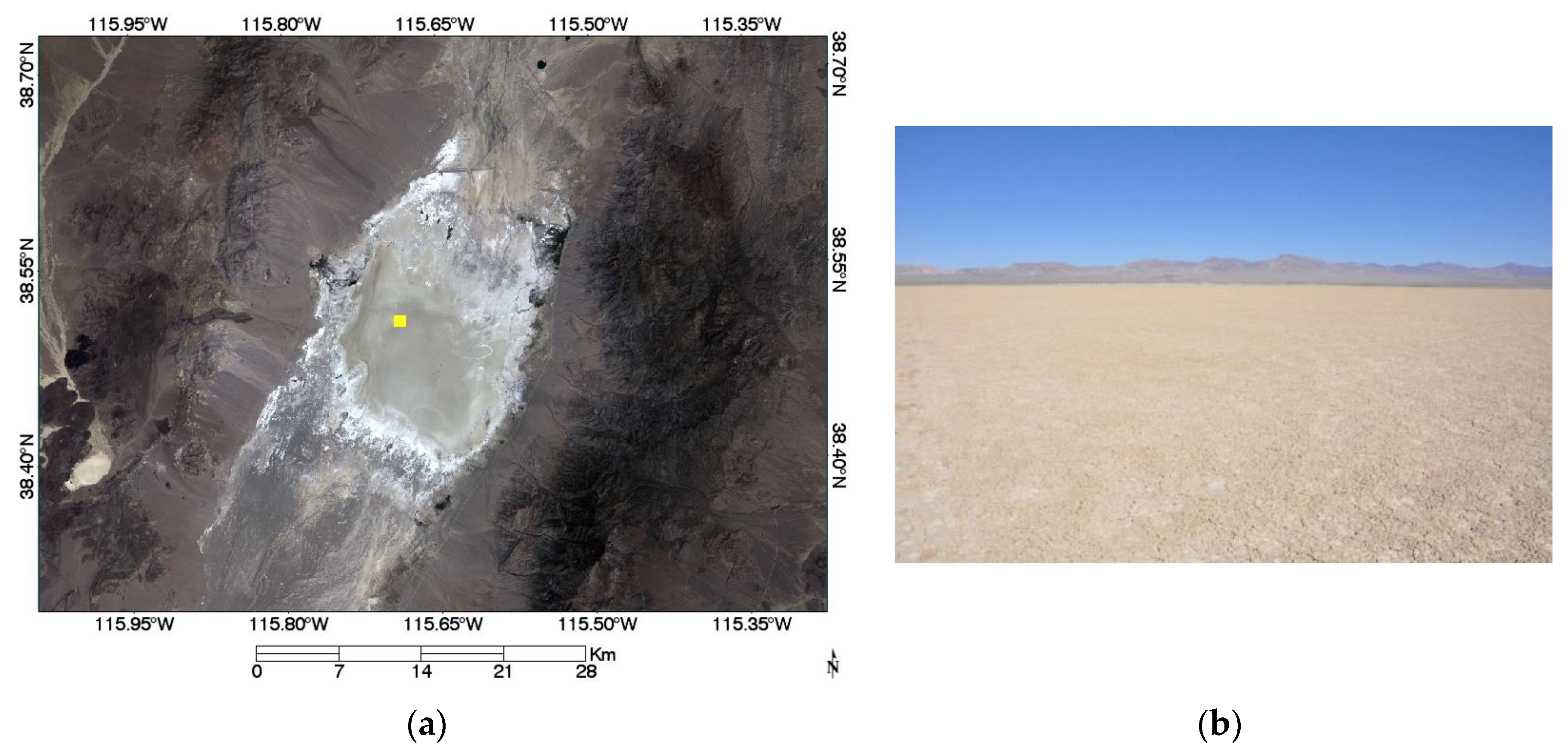
Railroad Valley Playa (RVUS) is currently maintained and operated by the University of Arizona (UoA) Remote Sensing Group (RSG). It also hosts an earlier RSG-developed automated network known as the Radiometric Calibration Test Site (RadCaTS) [3]. The instruments used to determine the surface reflectance are multispectral ground-viewing radiometers (GVRs), which were developed by the Remote Sensing Group at the UoA [4]. The RadCalNet TOA reflectance spectra are representative of a square 1 km × 1 km area centered at latitude 38.497° N and longitude 115.690° W, as shown by the yellow square in Figure 1a [4,5]. RVUS, located in Nevada, is a spatially homogenous section of dry lakebed, consisting of compacted clay-rich lacustrine deposits forming a relatively smooth surface, as seen in Figure 1b.

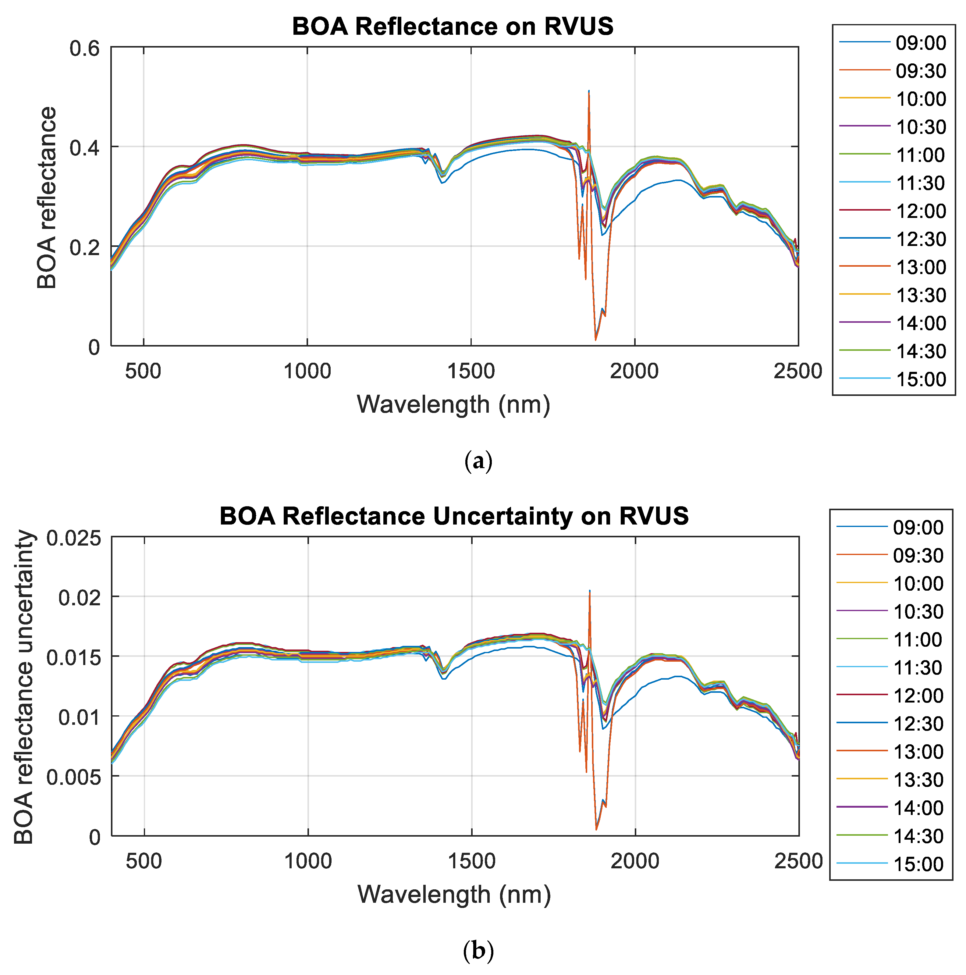
Figure 2a,b shows the measured surface (bottom of atmosphere (BOA)) reflectance at RVUS on 2015-07-15 and the associated uncertainties that are produced by the RadCalNet technical working group. The apparent change in reflectance throughout the day suggests a BRDF effect due to the changing position of the sun over time. Since BRDF effects come from variation in solar illumination and view geometries, on-orbit sensors acquiring data at off-nadir viewing angles should correct for them.

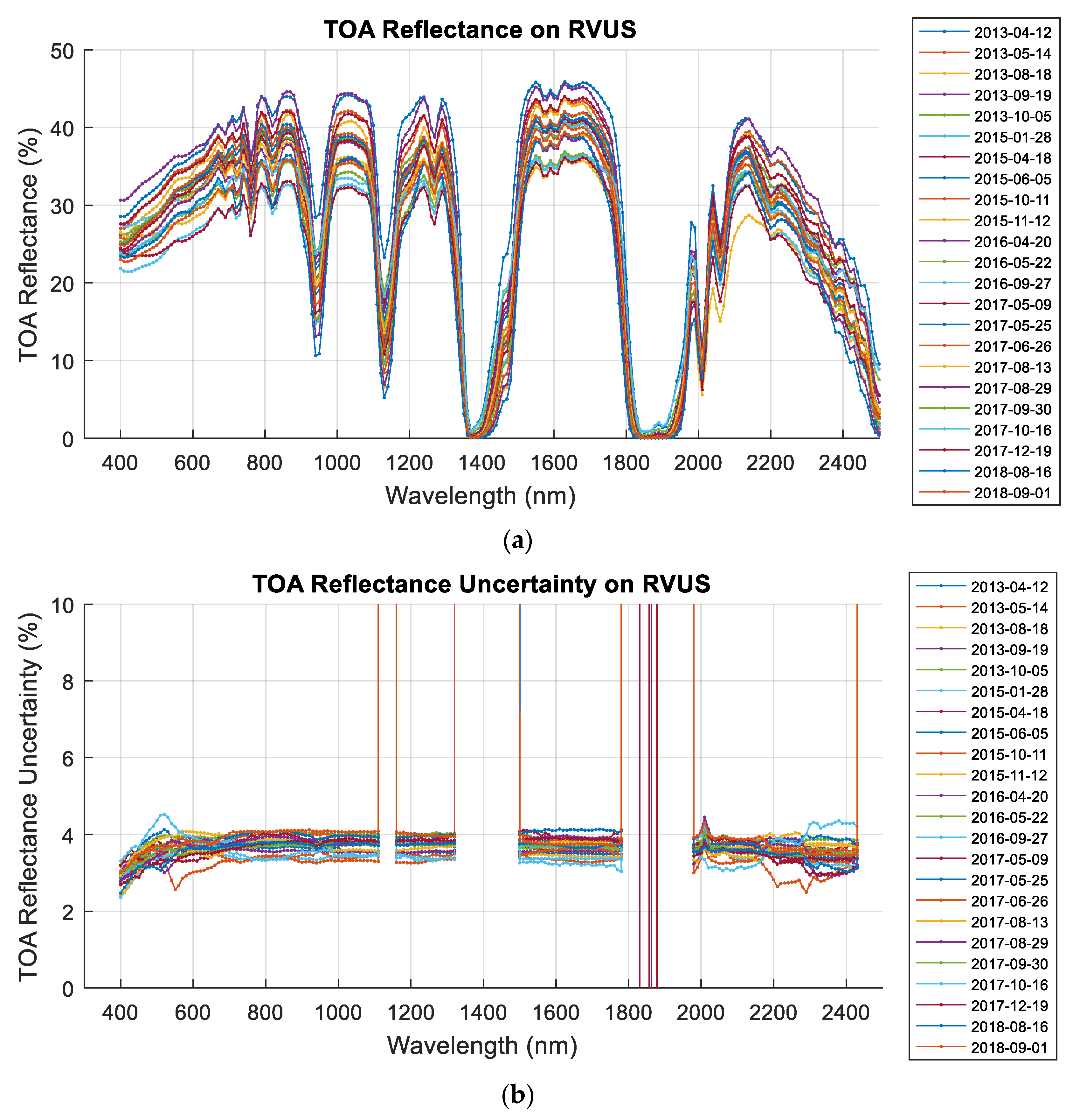
Figure 3a,b shows the TOA reflectance measured for cloud-free ETM+ overpasses between 2013 and 2018 at ~10:20 local standard time (~18:20 UTC) as well as the associated uncertainties that are produced by the RadCalNet technical working group. It can be seen in Figure 3a that the variation in measured TOA reflectance during this period is approximately 10% in the nonabsorption band regions, indicating that TOA reflectances vary with solar zenith angle. The associated uncertainties are consistently within 3% to 4%, indicating relative consistency in TOA reflectance measurements at this site.

2.1.2. La Crau (LCFR)

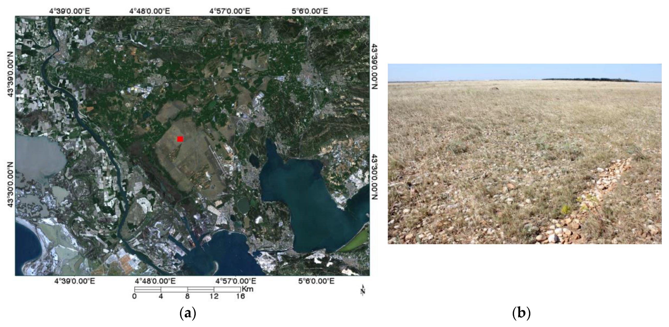
LCFR is located within the Reserve Naturelle des Coussouls de Crau Regional Park in France. The Centre National d’Etudes Spatiales (CNES) currently maintains and operates the instruments deployed at the site. The instruments used to determine the surface reflectance is Analytic Spectral Devices (ASD) FIELDSPEC-4 spectroradiometer mounted on a tripod with Spectralon panel as a reference [6]. The TOA reflectance spectra are representative of a disk of 30 m radius centered at latitude 43.552° N and longitude 4. 854° W, within a 1 km × 1 km area represented by the red square in Figure 4a [6]. Figure 4b shows a surface view of the site, which consists primarily of thin, pebbly soil with sparse vegetative cover.

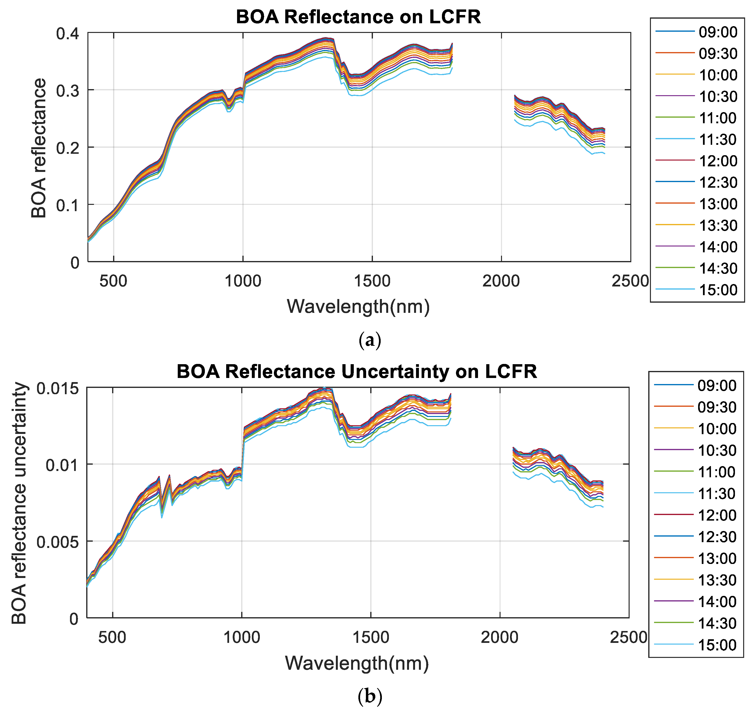
Figure 5a,b shows the surface reflectance measurements at LCFR acquired on 2015-06-02 and the associated uncertainties that are produced by the RadCalNet technical working group. Measurements from the atmospheric absorption wavelength ranges from 1820 nm to 2040 nm and 2410 nm to 2500 nm were removed due to excessive noise in the data. The ground measured reflectance changes as much as ~5% through the day due to changing solar illumination, suggesting again that BRDF effects are significant.

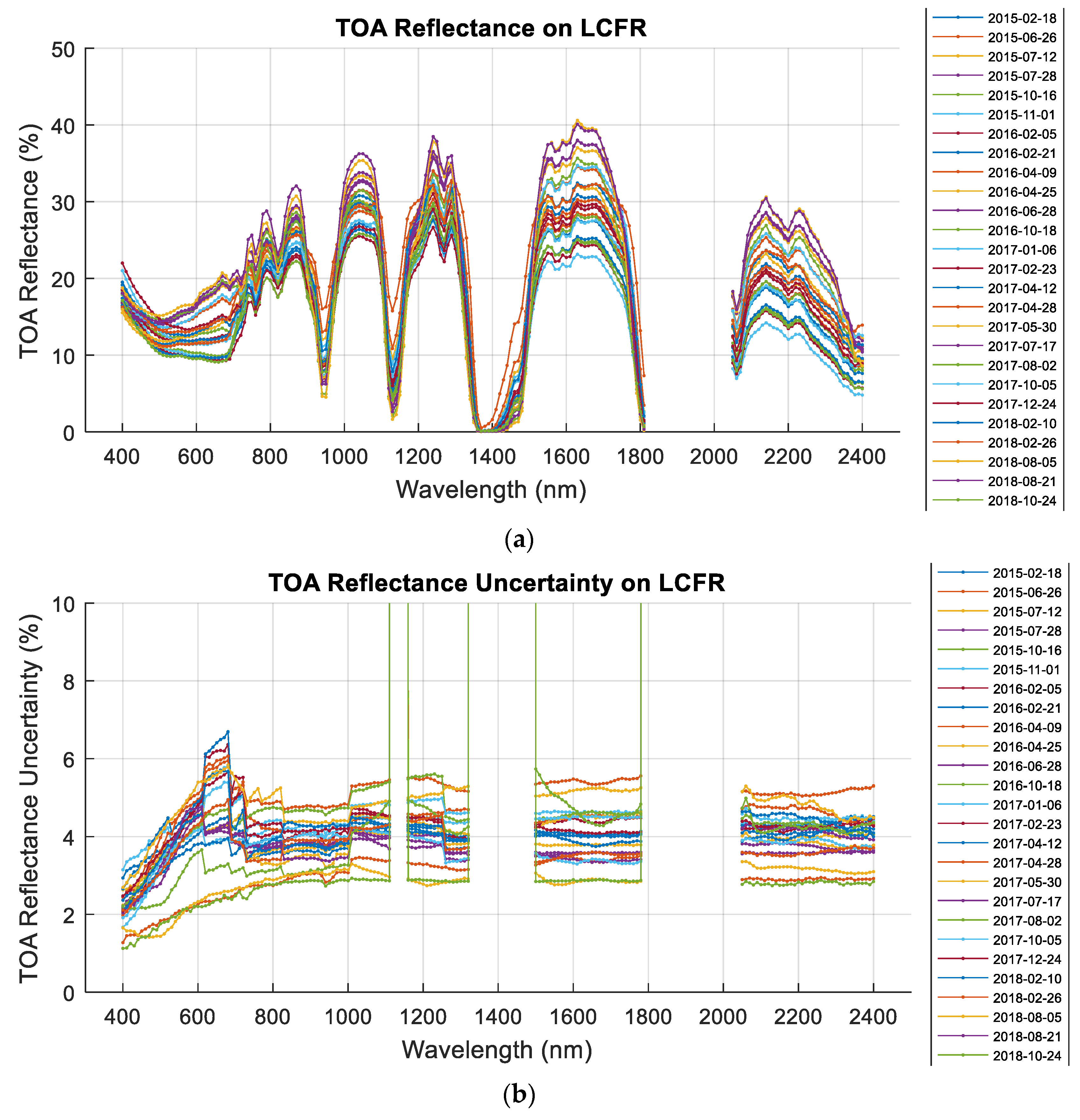
Figure 6a,b shows the TOA reflectance spectra for all cloud-free ETM+ overpasses at LCFR between 2015 and 2018 at ~10:20 local standard time (~10:20 UTC) as well as the associated uncertainties that are produced by the RadCalNet technical working group. Even though the acquisition period is shorter than that for RVUS, it is clearly seen in Figure 6a that the variation in TOA reflectance during this period is as high as 20% in the nonabsorption band regions. The corresponding uncertainties vary between approximately 2% and 6%, indicating that TOA reflectance at LCFR is less stable than at RVUS. This is not surprising, given that LCFR is a (minimally) vegetated site and RVUS is not.

2.1.3. Gobabeb (GONA)

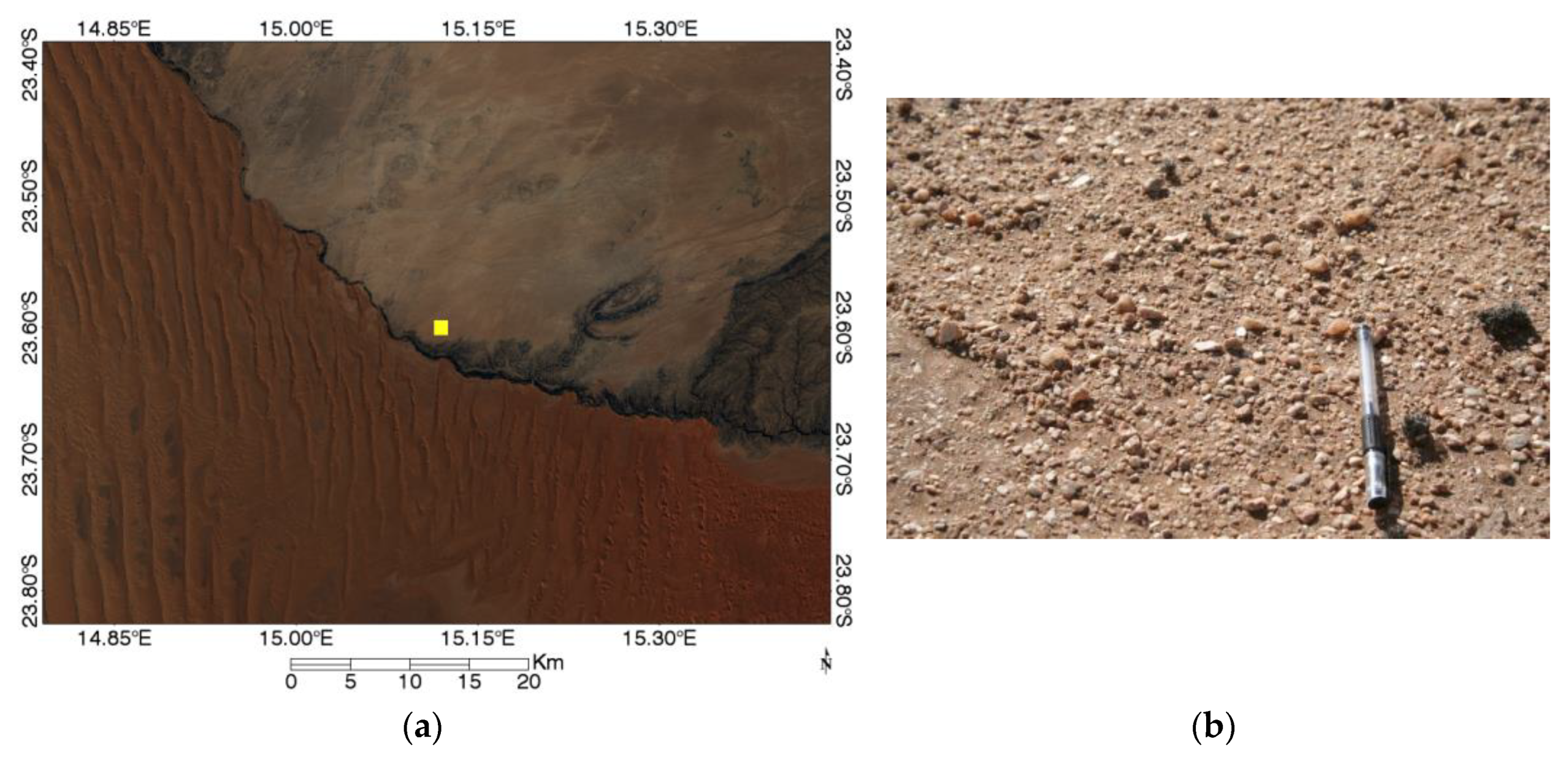
GONA is located near the Gobabeb Research and Training Centre in Namibia and is established as a joint European Space Agency (ESA) and CNES site, with the instruments maintained and operated by the National Physical Laboratory (NPL) in the UK on behalf of ESA. The instruments used to determine the surface reflectance is ASD spectroradiometer mounted on a tripod with Spectralon panel as a reference [7]. The TOA reflectance spectra are representative of a disk of 30 m radius centered at latitude 23.612° S and longitude 15.120° E, within a 1 km × 1 km area represented by the yellow square shown in Figure 7a [7]. The corresponding surface cover consists primarily of sand and gravel with some widely scattered dry grass, as seen in Figure 7b.

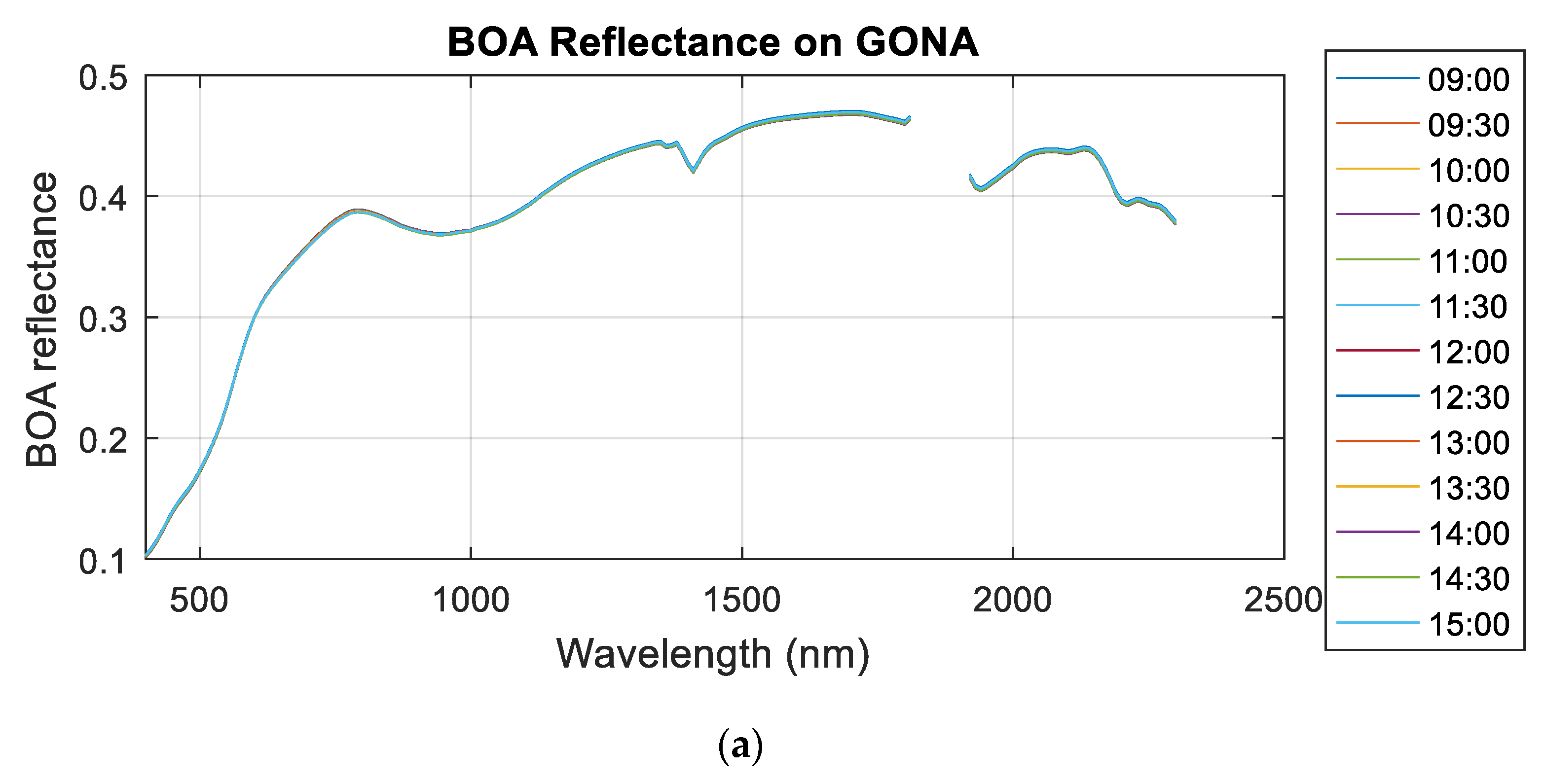
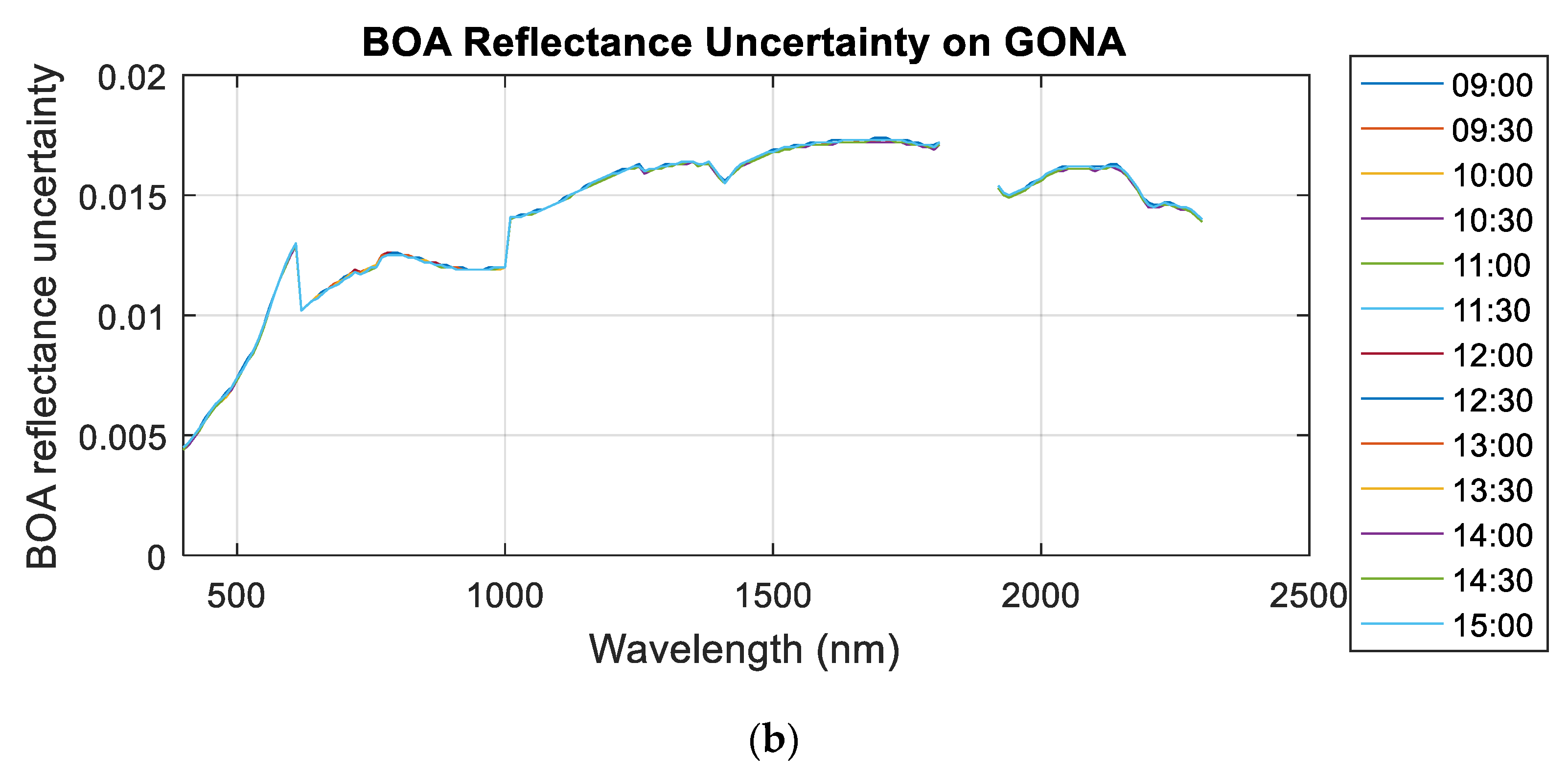
Figure 8a,b show measured surface reflectance at nadir view for GONA on 2017-08-08 and the associated uncertainties that are produced by the RadCalNet technical working group. Measurements from the absorption wavelength regions from 1820 nm to 1910 nm and 2300 nm to 2500 nm were excluded from the plot due to excessive noise in the data. The surface reflectance variation throughout the day is minimal, suggesting there are minimal or no BRDF effects needing correction.

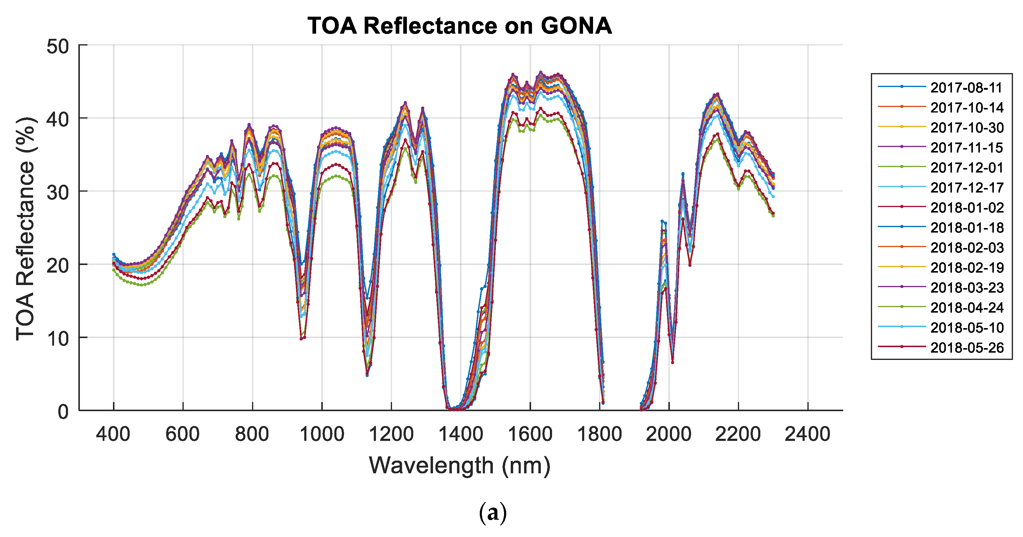
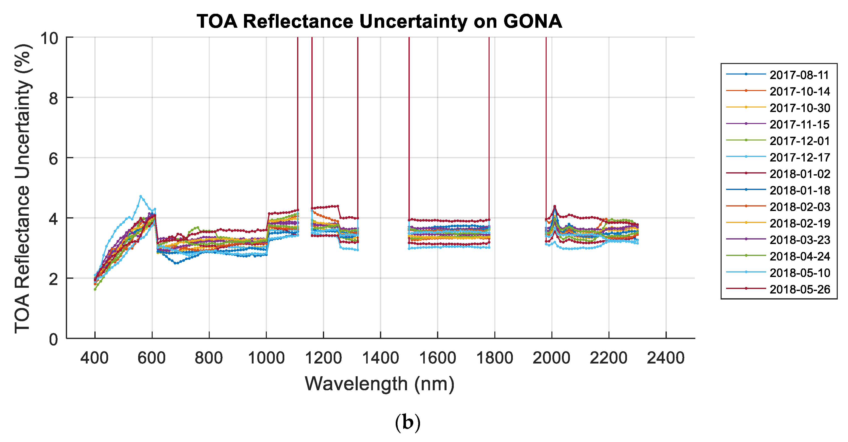
Figure 9a,b show TOA reflectance spectra for all cloud-free ETM+ overpasses of GONA from 2017 to 2018 at ~10:59 local standard time (~08:59 UTC) and the associated uncertainties that are produced by the RadCalNet technical working group. As with RVUS, the variation in TOA reflectance is within 10% during the acquisition period. The corresponding uncertainties are approximately 3% to 4%, indicating that reflectance measurements at GONA are relatively consistent.

2.2. Sensor Overview

Table 1. Sensor overview.

Satellite and Sensor
	Landsat 7 ETM+	Landsat 8 OLI	S2A MSI	S2B MSI
Launch date	1999-04-15	2013-02-11	2015-06-13	2017-03-07
Spectral bands (used in this study)	7 (7)	9 (8)	13 (11)	13 (11)
Pixel size (m)	30	30	10, 20, 60	10, 20, 60
Conversion to TOA reflectance equation *	${\rho }_{\lambda }=\frac{(M_{\rho }\times DN+A_{\rho })\times d^2}{\cos \left({\theta }_{\mathrm{SZA}}\right)}$ [8]		${\rho }_{\lambda }=DC/10000$ [9]

* $M_{\rho }$ is a band-specific multiplicative rescaling factor, $A_{\rho }$ is a band-specific additive rescaling factor, $d$ is Earth–Sun distance in astronomical units, ${\theta }_{\mathrm{SZA}}$ is the solar zenith angle for each pixel in the processed ROI, DN is the (calibrated) pixel digital values, $DC$ is the (calibrated) pixel digital count, and ${\rho }_{\lambda }$ is the final TOA reflectance. A metadata file included with the ETM+ and OLI image data products provides specific values for the rescaling factors.

provides the relevant background information for each sensor used in this study. Also included in the table are the equations used to convert the provided image data from calibrated DN values to TOA reflectance.

3. Methodology

This section describes the methodology used to conduct the study. Most of the processing steps are straightforward and require minimal description.

3.1. Data Selection

Each sensor’s imaging schedule was checked against the dates when RadCalNet data measurements were acquired. Overpass dates were selected when the site was imaged by a sensor of interest and RadCalNet acquired the corresponding surface measurements. The selected image datasets were downloaded from the sensor operator; ETM+, OLI, and MSI image data were downloaded through the US Geological Survey (USGS) EarthExplorer portal. All downloaded image data products were preprocessed by the sensor operator’s ground processing system with full radiometric correction and precision geometric registration/correction.

3.2. Cloud and Cloud Shadow Filtering

To screen out cloud effects, the maximum allowed cloud cover for the scenes retrieved from Earth Explorer was set at 10%. As cloud shadows may not be readily identified in the filtering, all downloaded images of the RadCalNet sites were visually inspected to ensure only cloud-free and shadow-free image data were used.

3.3. Image ROI Reflectance Extraction

Given the spatial resolution of the sensors and the representative region of the RadCalNet TOA reflectances, 30 pixel × 30 pixel (~1 km × 1 km) regions of interest (ROI) were selected for RVUS and 3 pixel × 3 pixel (~100 m × 100 m) ROI were selected for LCFR and GONA; these were centered at the representative region’s latitude/longitude coordinates given in Section 2. The cloud-free pixels from these ROIs were selected, then converted to TOA reflectances using the transformation equations provided in Table 1.

3.4. Image View Angle Effect Corrections

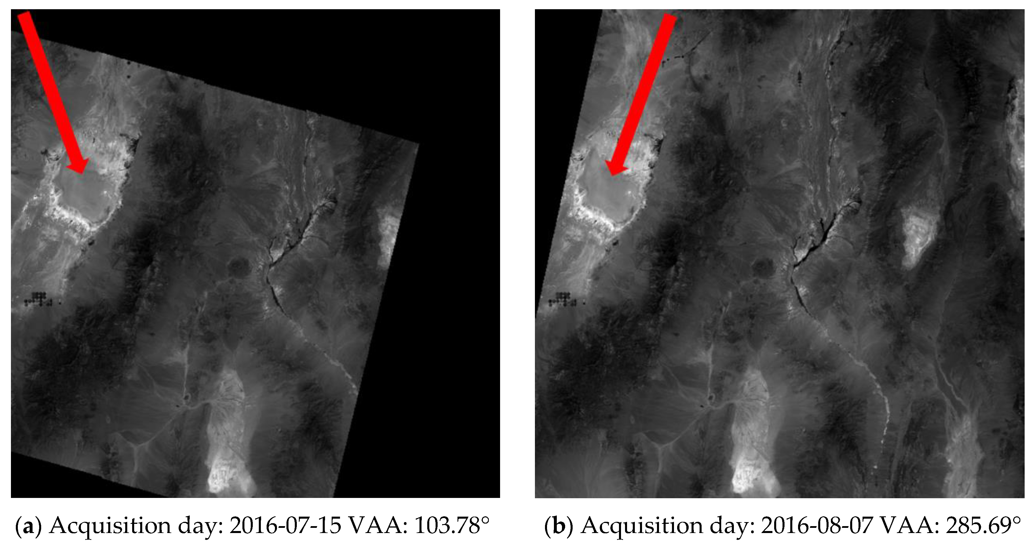
The RVUS, LCFR, and GONA sites are located in the ETM+ and OLI scene centers and the sensor zenith angles are no more than 0.1°; for these sensors, BRDF effects due to the view angle could be considered insignificant. However, for the MSI sensors, the RVUS and LCFR sites are located in overlapping orbital swaths (Figure 10), thus requiring application of a viewing angle effect correction.

A simple series of steps was performed to correct the viewing angle effect [10]. First, to obtain the correction coefficients $a_{\lambda }$ and $b_{\lambda }$, a linear regression was performed on the observed TOA reflectances versus the variable $x$:

$${\rho }_{i,\lambda }^{\mathrm{MSI}}=a_{\lambda }\times x+b_{\lambda },$$

(1)

where ${\rho }_{i,\lambda }^{\mathrm{MSI}}$ is the MSI TOA reflectance on date $i$ measured for band $\lambda$, and the variable $x$ is defined as follows

$$x=\sin {\theta }_{\mathrm{z}}\cos {\theta }_{\mathrm{a}},$$

(2)

where ${\theta }_{\mathrm{z}}$ and ${\theta }_{\mathrm{a}}$ are the sensor viewing zenith and viewing azimuth angles, respectively. A “reference” TOA reflectance ${\rho }_{\lambda }^{\mathrm{r}}$ was then estimated from the mean reflectance of band $\lambda$ across all dates. Finally, the corrected reflectance ${\rho }_{i,\lambda }^{\mathrm{c}}$ was calculated as the ratio of the observed and regression-predicted TOA reflectances scaled by the “reference” reflectance:

$${\rho }_{i,\lambda }^{\mathrm{c}}=\frac{{\rho }_{\lambda }^{\mathrm{r}}\times {\rho }_{i,\lambda }^{\mathrm{MSI}}}{a_{\lambda }\times x+b_{\lambda }},$$

(3)

Note that in order to compare the effectiveness of this viewing angle effect correction method for MSI sensors, a set of results were made without that correction as described in Section 4.1 and Section 4.2, and then this method was applied to the measurements.

3.5. RadCalNet Reflectance Extraction

First, the TOA reflectance data from each RadCalNet site were extracted. Second, the extracted spectra were linearly interpolated to estimate the TOA reflectance at the sensor overpass times. Third, interpolated the relative spectral response of the sensors from 1 nm to 10 nm to match the spectral resolution of RadCalNet spectral data. Lastly, the RadCalNet spectral measurements were normalized to the corresponding multispectral value for the sensor of interest in order to allow direct comparison to the sensor-measured TOA reflectance:

$${\rho }_{\mathrm{RCN}}=\frac{{\displaystyle \sum _{\lambda 1}^{\lambda 2}{\rho }_{\lambda }^{\mathrm{H}}\times SR{F}_{\lambda }}}{{\displaystyle \sum _{\lambda 1}^{\lambda 2}SR{F}_{\lambda }}},$$

(4)

where ${\rho }_{\lambda }^{\mathrm{H}}$ is the RadCalNet TOA spectral reflectance, $SR{F}_{\lambda }$ is the relative spectral response function of the sensor, and ${\lambda }_1$ and ${\lambda }_2$ define the band of interest with 10 nm steps. ${\rho }_{\mathrm{RCN}}$ is the integrated equivalent reflectance of the RadCalNet-predicted TOA reflectance in the specific sensor band.

3.6. Reflectance difference Analysis

In this study, both the relative TOA reflectance difference and the standard deviation of the difference were used as an index to evaluate the reliability of the RadCalNet sites. The relative difference (as a percentage) was calculated as

$$\Delta \rho \%=\frac{{\rho }_{\mathrm{S}}-{\rho }_{\mathrm{RCN}}}{{\rho }_{\mathrm{RCN}}}\times 100\%$$

(5)

where ${\rho }_{\mathrm{S}}$ is the sensor-measured TOA reflectance, ${\rho }_{\mathrm{RCN}}$ is the corresponding RadCalNet-predicted TOA reflectance, and $\Delta \rho \%$ is the relative difference in TOA reflectance.

From the processing procedure described above, a time series of relative TOA reflectance difference data points were generated for each RadCalNet site. To quantitatively indicate the variation of the results for comparisons between the sites, the TOA reflectance difference standard deviation was calculated as follows

$$\sigma =\sqrt{\frac{1}{n-1}{\displaystyle \sum }_{k=1}^n{\left(\Delta {\rho }_k-\overline{\Delta \rho }\right)}^2}$$

(6)

where $\sigma$ is the TOA reflectance difference uncertainty of the site and $n$ is the number of overpass events at each site.

3.7. TOA Reflectance Comparison Uncertaity Analysis

To quantitatively indicate the comparison results among the sites, the TOA reflectance comparison uncertainties were performed considering five sources of uncertainties associated (i) uncertainty from the RadCalNet predicted reflectance, (ii) uncertainty from spectral response function, (iii) uncertainty from temporal linear interpolation, (iv) uncertainty from spectral interpolation, and (v) sensor calibration uncertainties, which are approximately 5%, 3%, and 4% for ETM+, OLI, and both MSIs, respectively, as reported in Chander, G., etc., Mishra, N., etc., and Czapla-Myers, J., etc. [11,12,13]. To calculate the total uncertainty, first, uncertainties (i) and (ii) were propagated through Equation (4) using a Monte Carlo simulation method [14], assuming spectral correlation matrix (correlation between the wavelengths) values were decreasing in the subdiagonal, adjacent to the main diagonal, ranging from 0.9 to 0.1, with an interval of 0.1; the remaining correlation value used to fill up the matrix was 0.05 (the correlation in the main diagonal equal to 1). Second, for the uncertainty associated with temporal linear interpolation, is was assumed that the RadCalNet predicted values before and after the sensor over pass time are the variation limitations of the temporal interpolated TOA reflectance, then the reflectance error between before/after values and the interpolated values are calculated, the larger absolute error was indicated as the uncertainty associated with temporal interpolation. Third, the spectral resolution uncertainty has been assumed as 0.25% for all bands based on previous work [15]. Last, assuming independence among the uncertainty sources (except (i) and (ii)), the final uncertainties were calculated.

4. Results

4.1. Comparison of RVUS Results

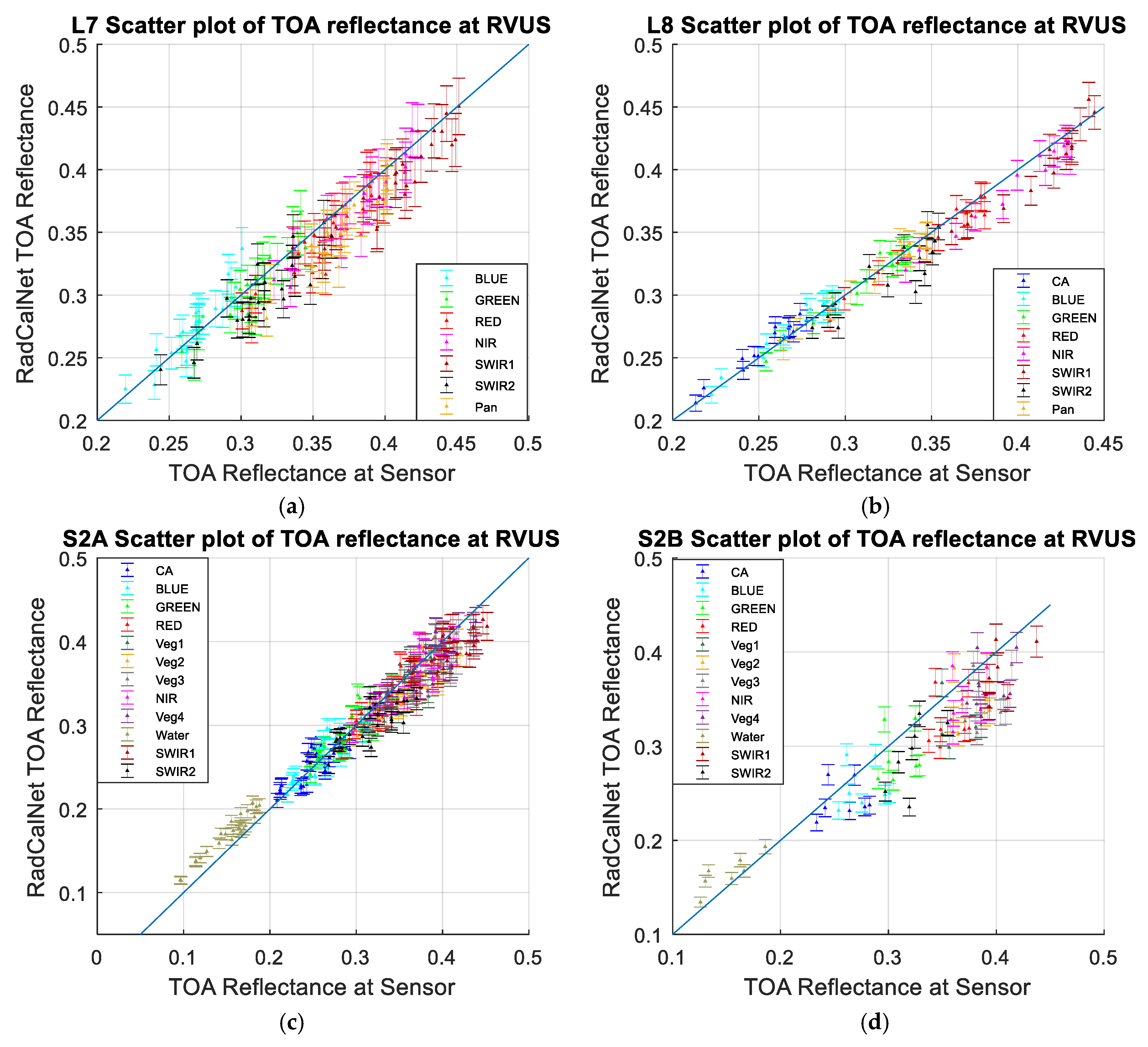
Figure 11a–d shows scatterplots of the RadCalNet predicted TOA reflectances and the corresponding sensor-measured TOA reflectances. The error bars in each figure represent the overall uncertainty of each data point that discussed in Section 3.7. The blue line in each figure is a standard 1:1 line.

In general, the 1:1 lines for ETM+ and OLI fall within the estimated uncertainty range in all bands for most of the data points. However, the lines tend to lie at the lower ends of the range at shorter wavelengths and at the upper end of the range at longer wavelengths. For the MSI sensors, two states can be observed in the data: (i) a net offset above the 1:1 line in the water band (indicating the RadCalNet-predicted TOA reflectance is greater than the value measured by the sensor) and (ii) a net offset below the 1:1 line in the SWIR bands (indicating that the sensor-measured TOA reflectance is greater than the RadCalNet-predicted value). The overall scatter of the data about the 1:1 line appears to be more pronounced in the S2B MSI data, part of this reason may be due to the reduced amount of data relative to the other sensors; the general pattern in its data is consistent with that observed for S2A MSI.

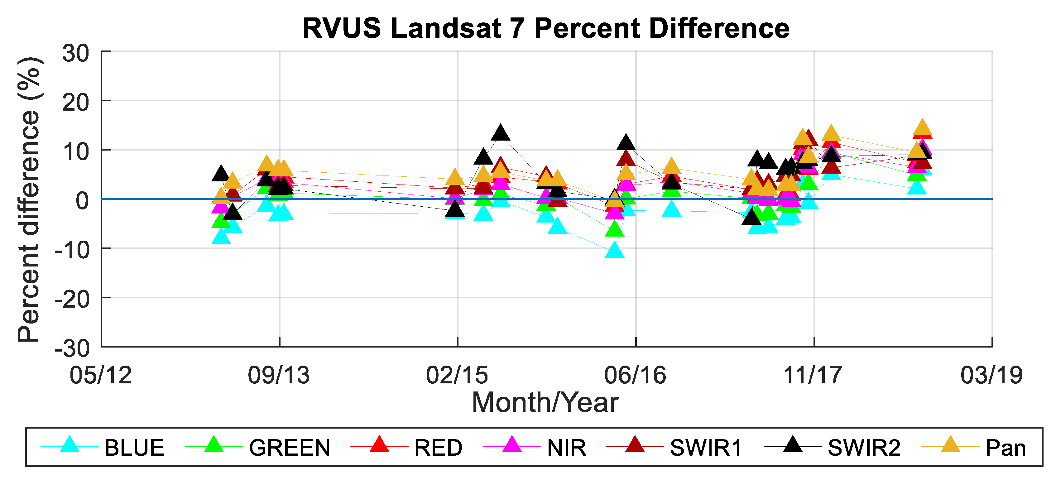
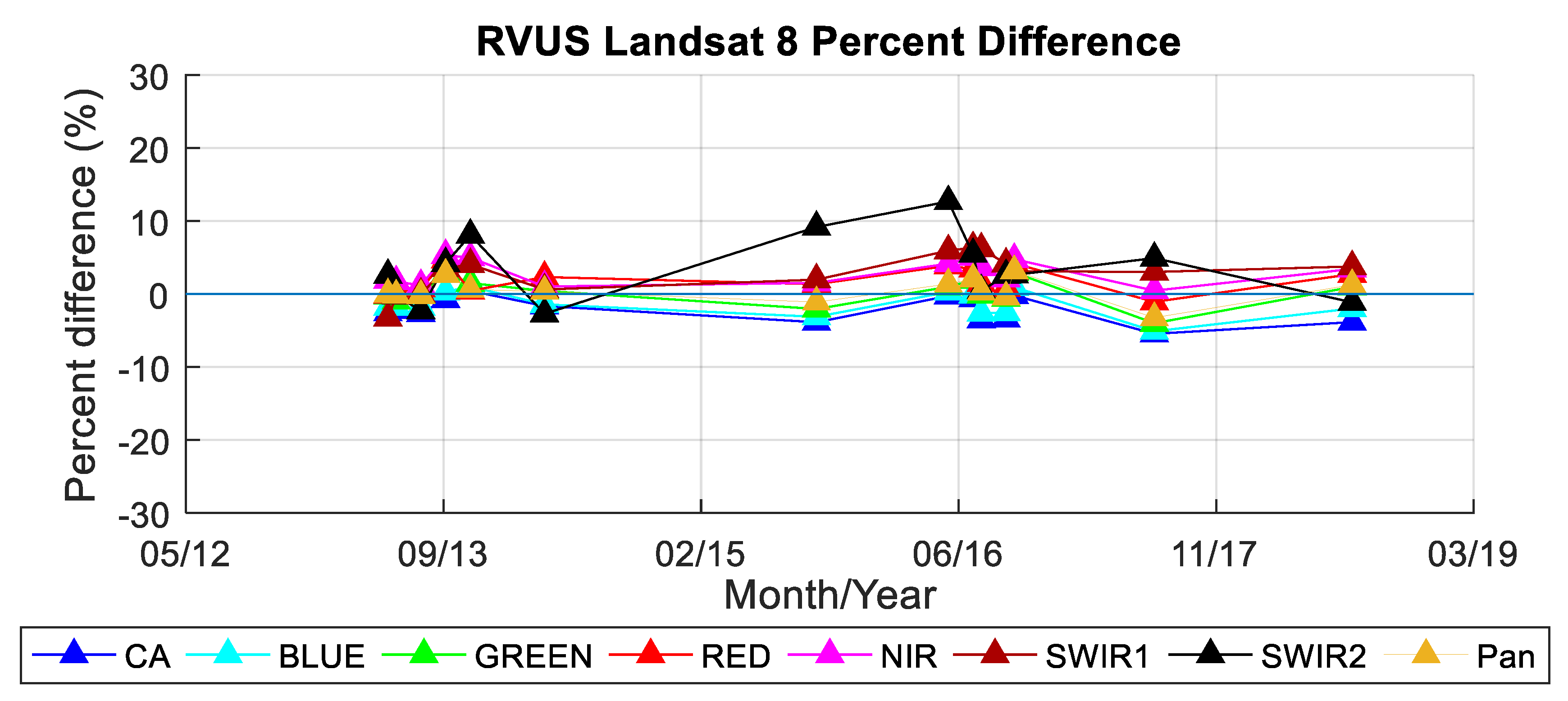
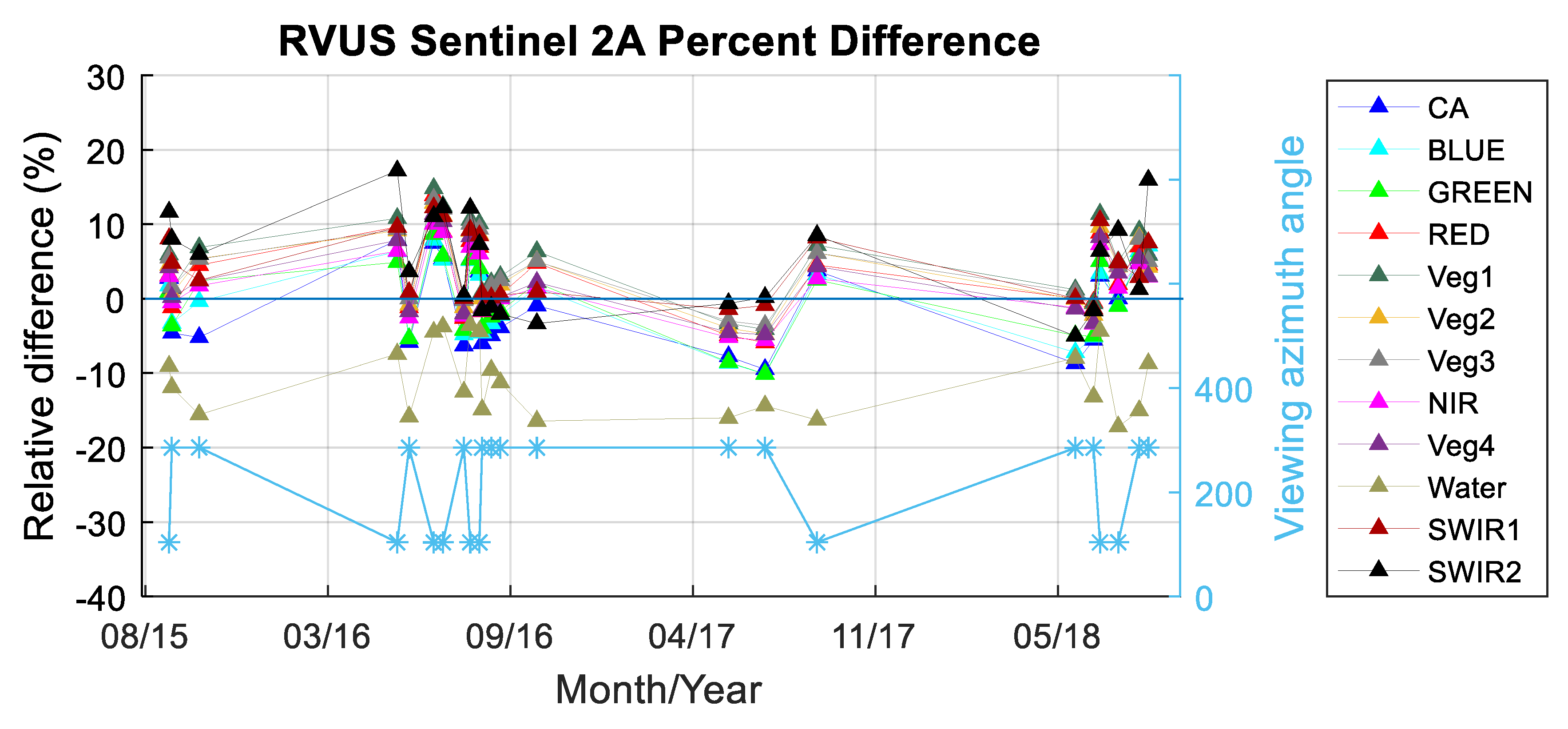
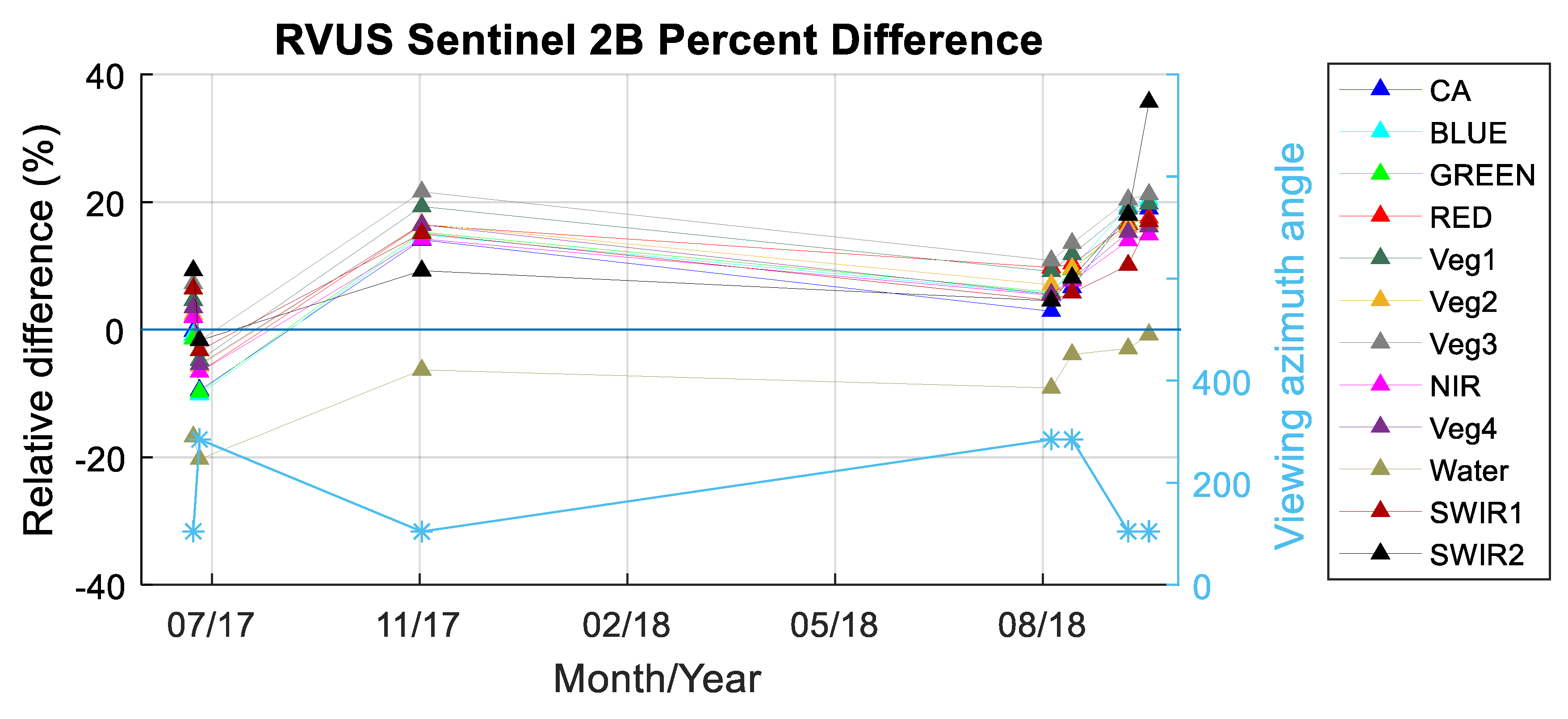
Figure 12, Figure 13, Figure 14 and Figure 15 show the relative TOA reflectance difference results between RadCalNet and ETM+, OLI, S2A MSI, and S2B MSI, respectively, without viewing angle correction. In general, the relative differences for ETM+, OLI, and S2A MSI are within ±10%; for the S2A MSI water band, the differences are within −20% and 0%. For S2B MSI, the relative differences are generally between 0% and 20% in all bands except the water band, where the differences are within −20% and 0%. Interestingly, the reflectance differences in the MSI sensors exhibit an “up and down” behavior not seen in the ETM+ and OLI reflectance differences.

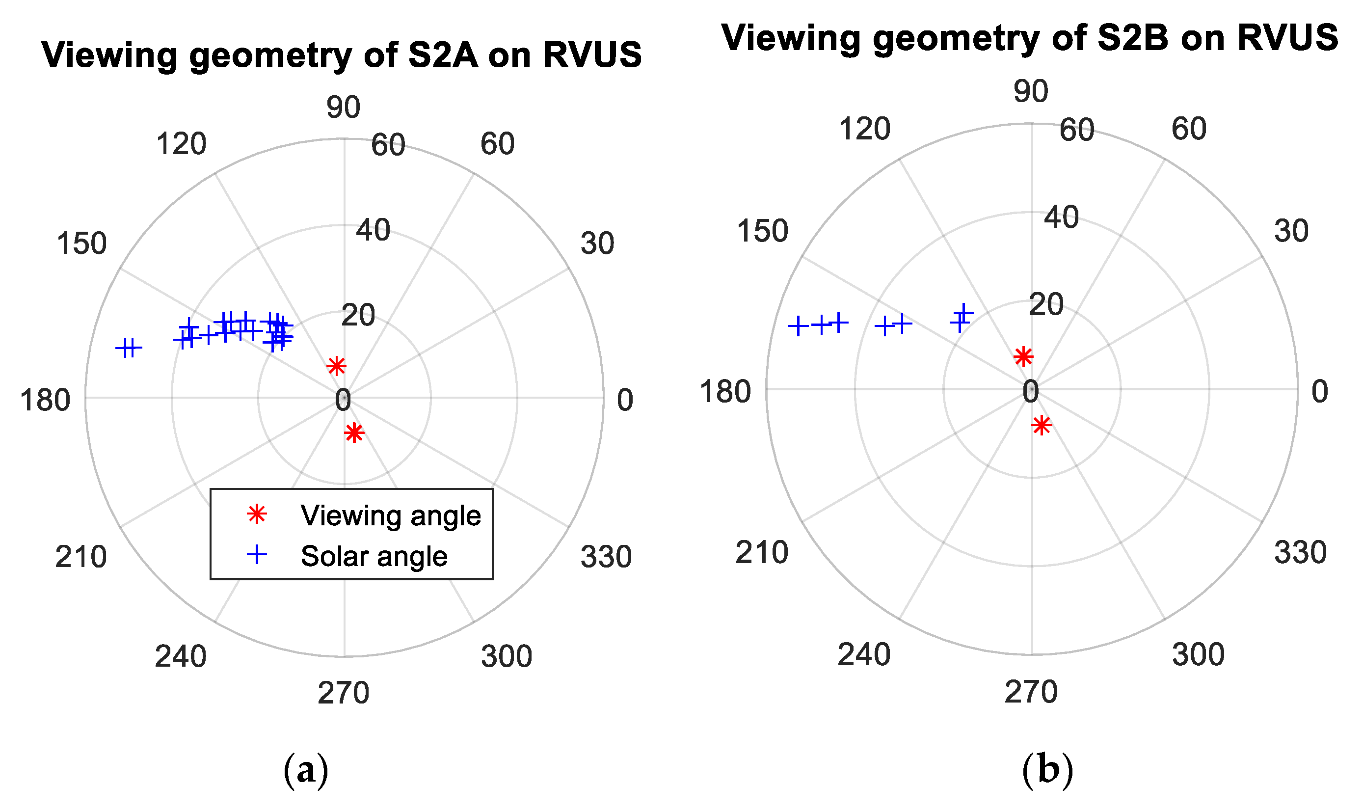
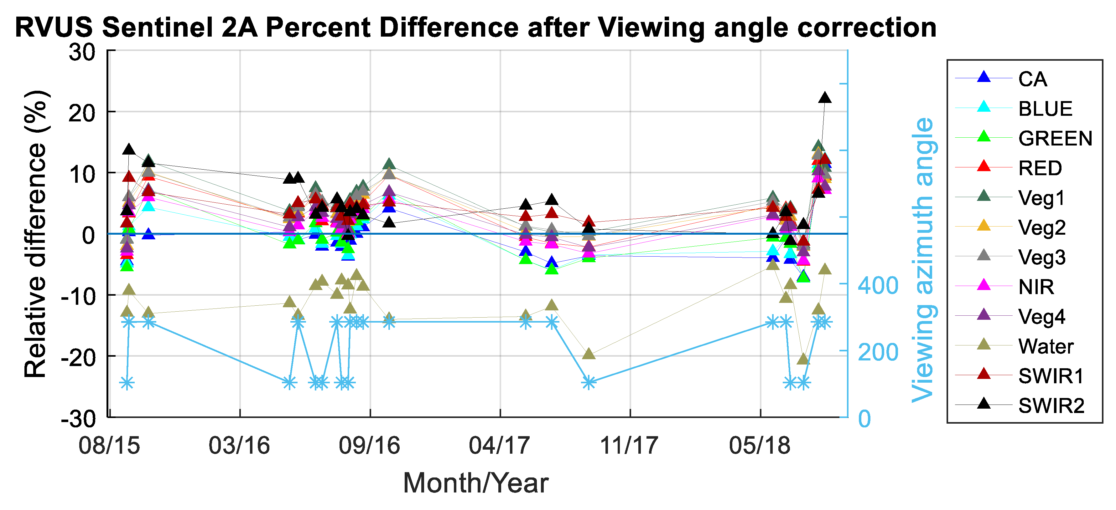
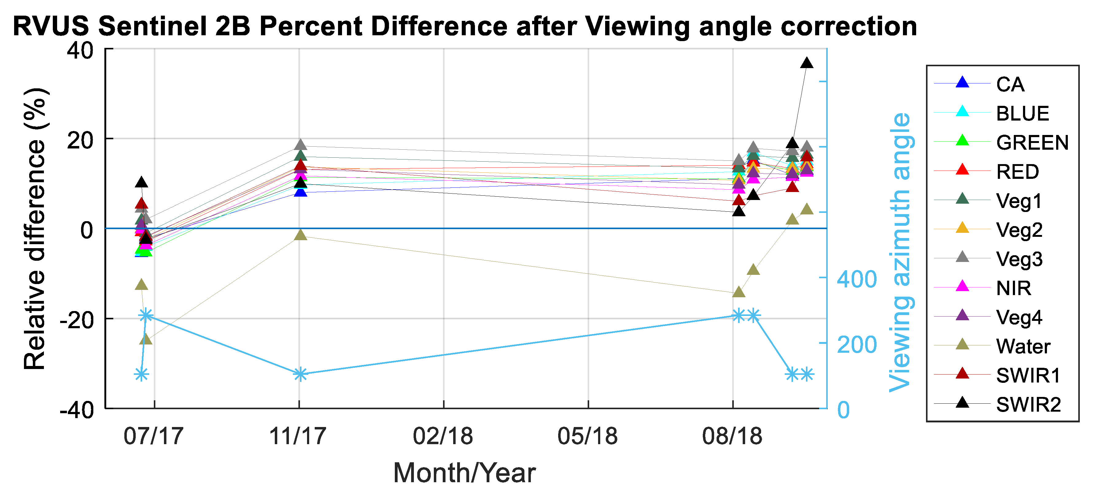
Further investigation into the apparent oscillatory behavior in the MSI relative TOA reflectance differences suggests that differences in the individual MSI viewing geometries is the most likely reason. Figure 16a,b shows polar plots of the available sensor view angle (red asterisks) and solar illumination angle (blue plus signs) for S2A and S2B at RVUS (with the zenith angles represented by circles of increasing radii). The viewing azimuth angles for both MSIs are located in opposite directions due to overlapping swaths from adjacent orbits. Figure 17 and Figure 18 show the viewing azimuth angle (VAA) against the relative reflectance difference of the two Sentinel sensors. The relationship between the relative reflectance difference and the viewing azimuth is obvious. Therefore, the correction described in Section 3.4 was applied.

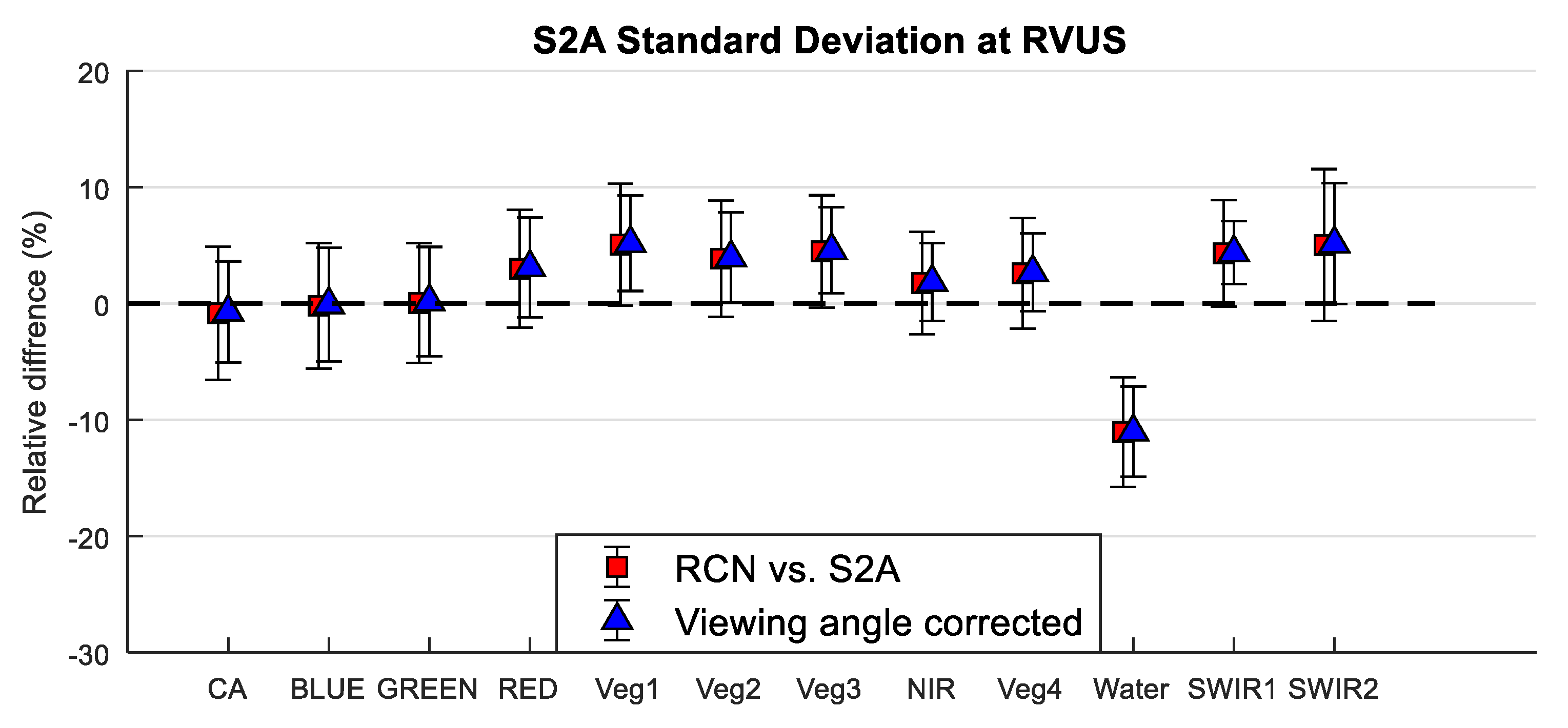
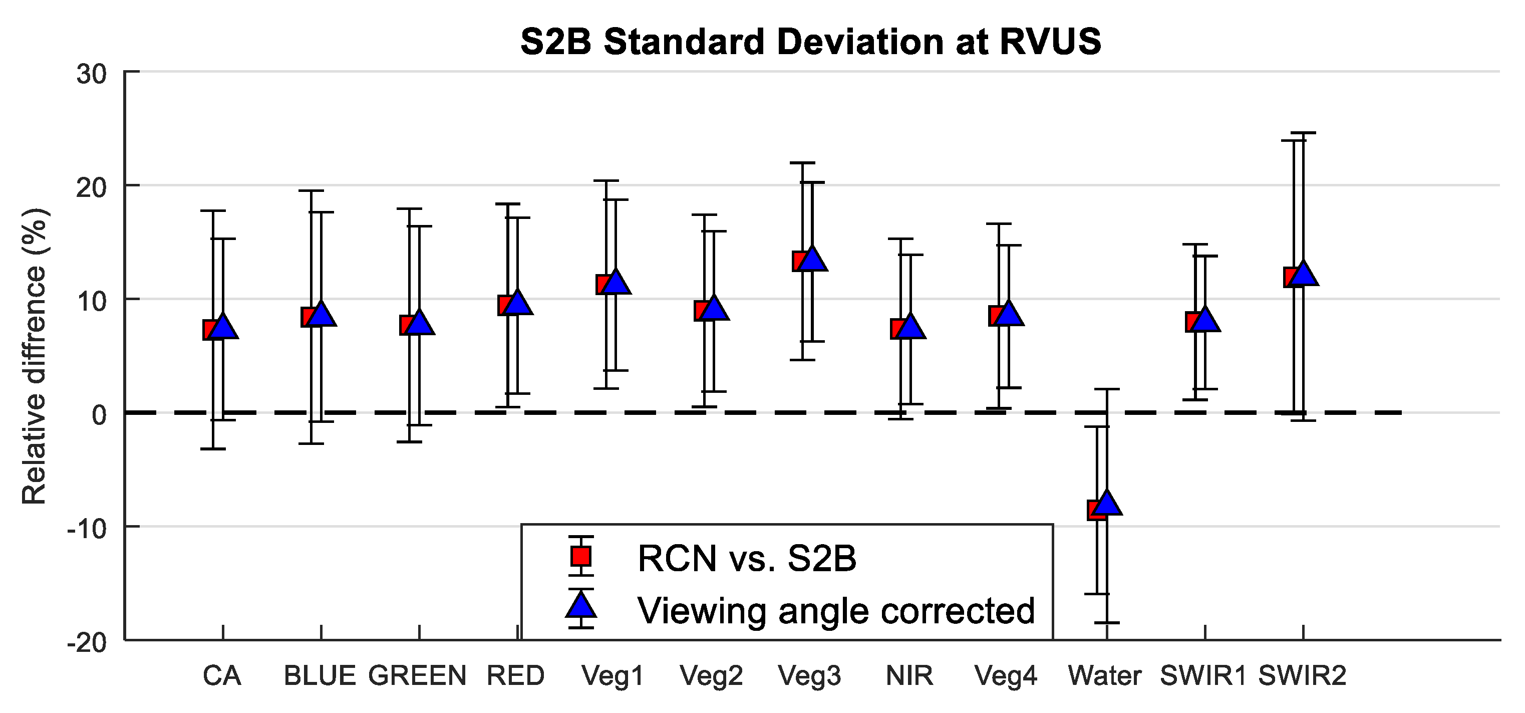
Figure 17 and Figure 18 show the MSI relative reflectance data after application of the view angle effect correction method. The correction significantly reduces the impact of the viewing azimuth angle related effect. Figure 19 and Figure 20 show the average relative TOA reflectance differences with standard deviation for each MSI at RVUS before and after application of the viewing angle effect correction. The average relative difference before and after correction does not significantly change; however, the standard deviation of the differences reduces to approximately 1% in all bands except the water and SWIR 2 bands in S2B MSI. As indicated earlier, the higher variability in the S2B MSI data is most likely due to its much smaller lifetime dataset compared to the other sensors.

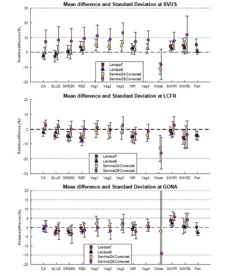
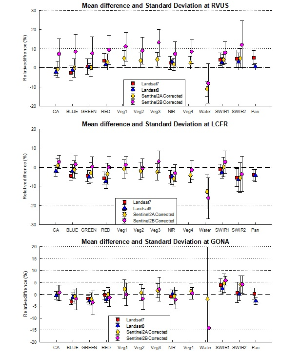
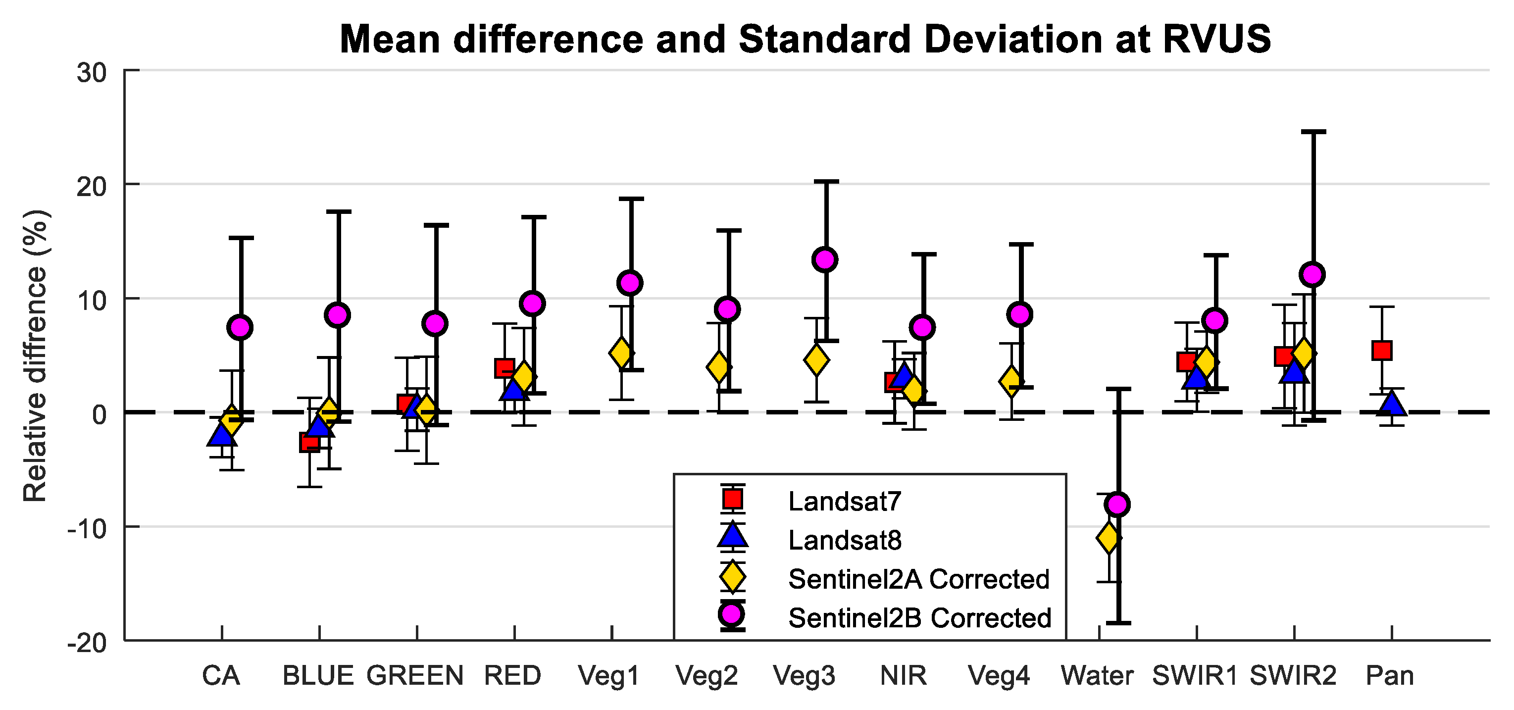
Figure 21 shows the relative TOA reflectance difference standard deviation between RadCalNet and ETM+, OLI, and S2A/2B MSI (after application of the viewing angle effect correction) at RVUS.

Table 2. Number of overpass dates, mean relative reflectance difference, and standard deviation for each sensor, RVUS.

Diff% ± Standard Deviation%
	ETM+	OLI	S2A MSI After Viewing Angle Effect Correction	S2B MSI After Viewing Angle Effect Correction
# of Overpasses	23	14	23	7
CA	N/A	−2.2 ± 1.7	−0.7 ± 4.4	7.3 ± 8.0
Blue	−2.6 ± 3.9	−1.4 ± 1.7	−0.1 ± 4.9	8.4 ± 9.2
Green	0.7 ± 4.1	0.2 ± 1.9	0.2 ± 4.7	7.6 ± 8.8
Red	3.9 ± 3.9	1.8 ± 1.8	3.1 ± 4.3	9.4 ± 7.7
Veg1	N/A	N/A	5.2 ± 4.1	11.2 ± 7.5
Veg2	N/A	N/A	4.0 ± 3.9	8.9 ± 7.0
Veg3	N/A	N/A	4.6 ± 3.7	13.3 ± 7.0
NIR	2.6 ± 3.6	3.0 ± 1.7	1.9 ± 3.3	7.3 ± 6.5
Veg4	N/A	N/A	2.7 ± 3.3	8.4 ± 6.3
Water	N/A	N/A	−11.0 ± 3.9	−8.2 ± 10.3
SWIR 1	4.4 ± 3.4	2.8 ± 2.8	4.4 ± 2.7	7.9 ± 5.8
SWIR 2	4.9 ± 4.5	3.3 ± 4.5	5.2 ± 5.2	11.9 ± 12.7
Pan	5.4 ± 3.8	0.5 ± 1.6	N/A	N/A

summarizes the number of overpasses and the corresponding mean and standard deviation of the band-specific TOA relative reflectance differences for each sensor.

The mean relative TOA reflectance difference of ETM+, OLI, and S2A MSI are generally within ± 6% across all bands. This is not the case for the water band of S2A MSI, which has differences of –11.0% ± 3.9%. The mean relative reflectance difference of S2B, however, is within 7% to 13.3% in all bands except the water band, which has a difference of approximately –8.2% ± 10.3%. With respect to the standard deviation, OLI has the smallest deviation, ETM+ and S2A MSI are comparable, and S2B MSI has the largest standard deviation, which is not surprising given its small number of available overpasses at RVUS.

Based on the consistency of results among ETM+, OLI, and S2A MSI, it could be concluded that RVUS can yield consistent, NIST-traceable calibration results for both a sensor and the site itself.

4.2. Comparison of LCFR Results

Similar comparisons were made to evaluate the LCFR data. As is the case with RVUS, LCFR is also located in the ETM+ and OLI scene centers and the sensor zenith angles are no more than 0.1°. For the MSI sensors, the site is also located in overlapping orbital swaths, thus requiring application of the viewing angle effect correction.

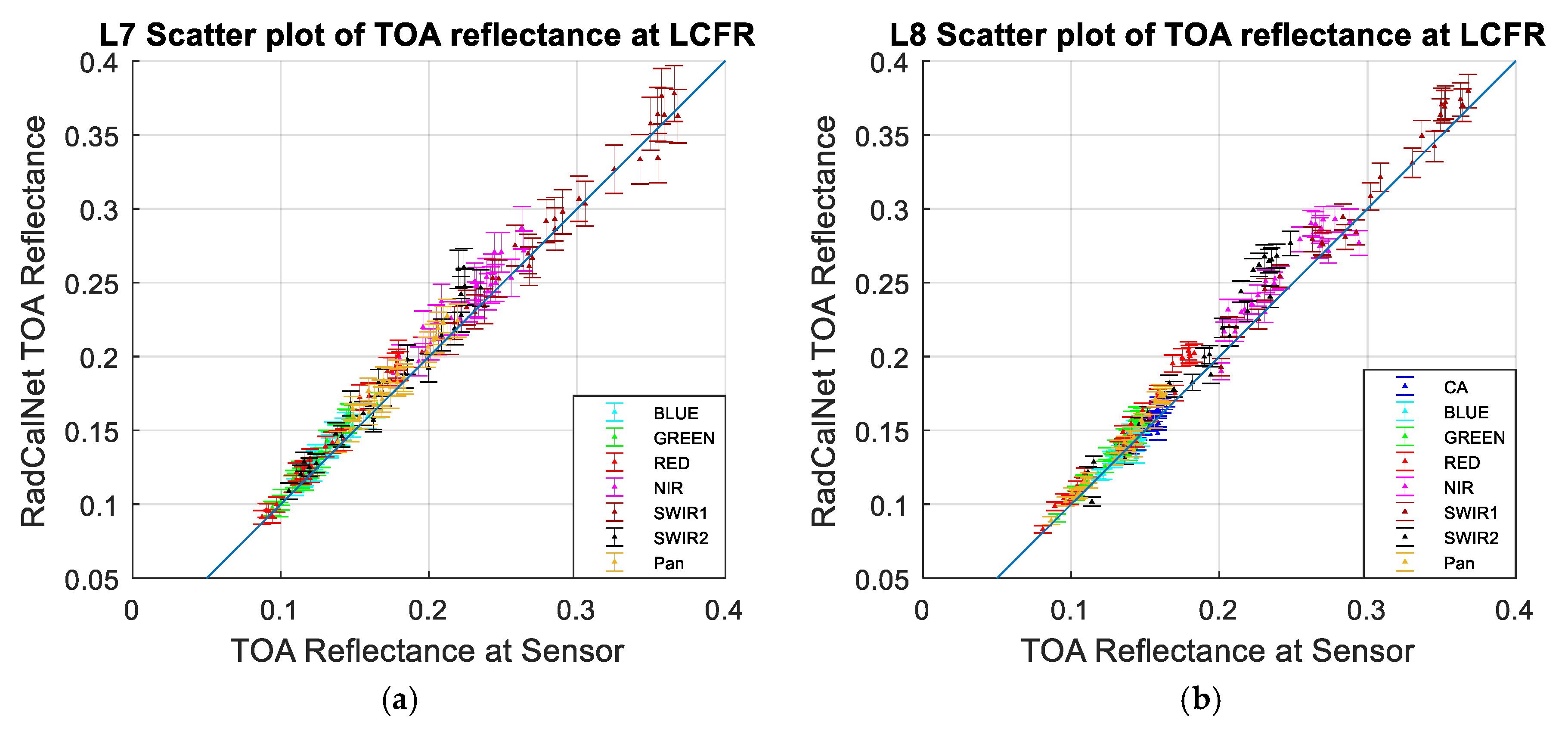
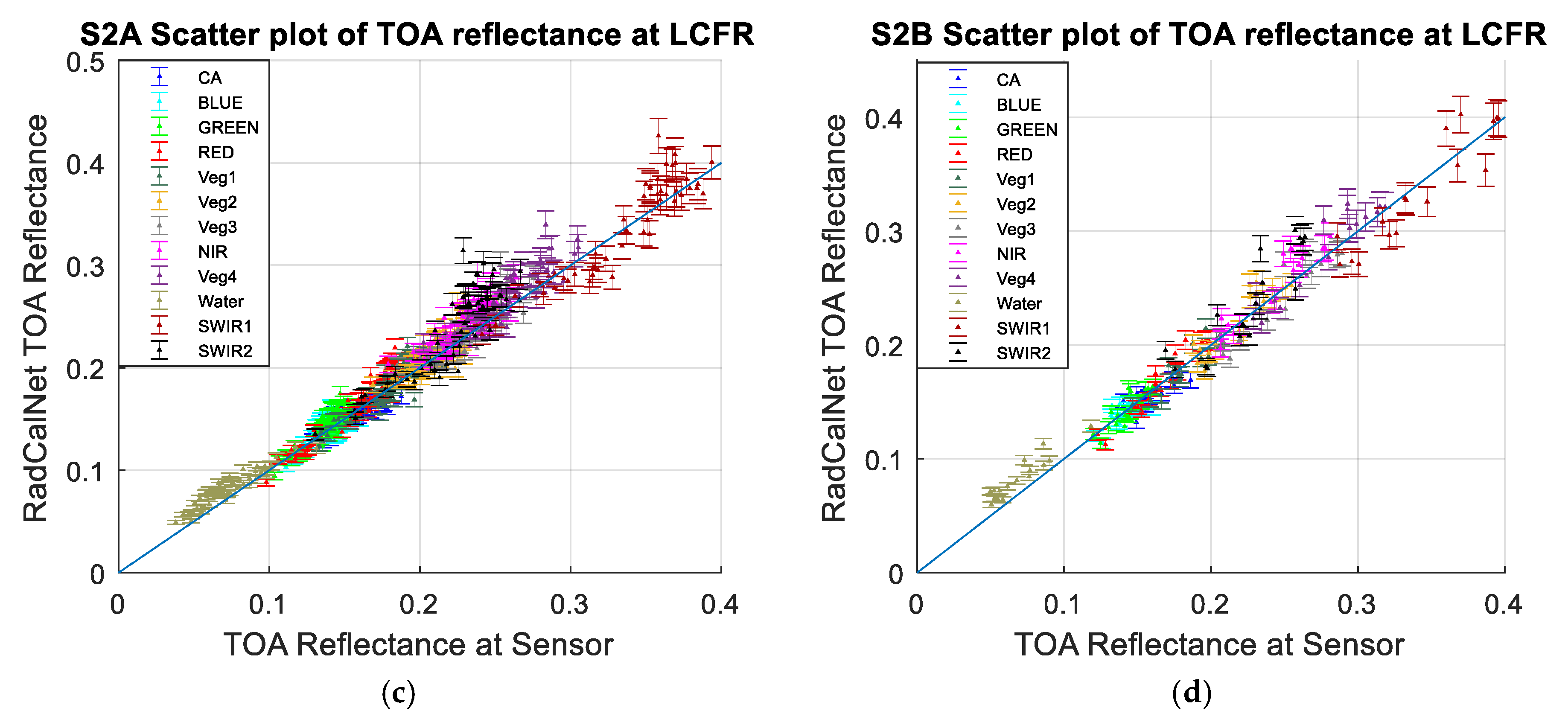
Figure 22a–d shows scatterplots of the RadCalNet-predicted TOA reflectances and the corresponding sensor-measured TOA reflectances at LCFR; as before, the blue line is the standard 1:1 line. Figure 22c,d shows the MSI scatterplots before application of the viewing angle effect correction. For ETM+ and OLI, most of the data points consistently lie above the 1:1 line, indicating the predicted TOA reflectance is higher than the measured ETM+ and OLI values. For MSI sensors, the data points are not as concentrated in the longer wavelength bands.

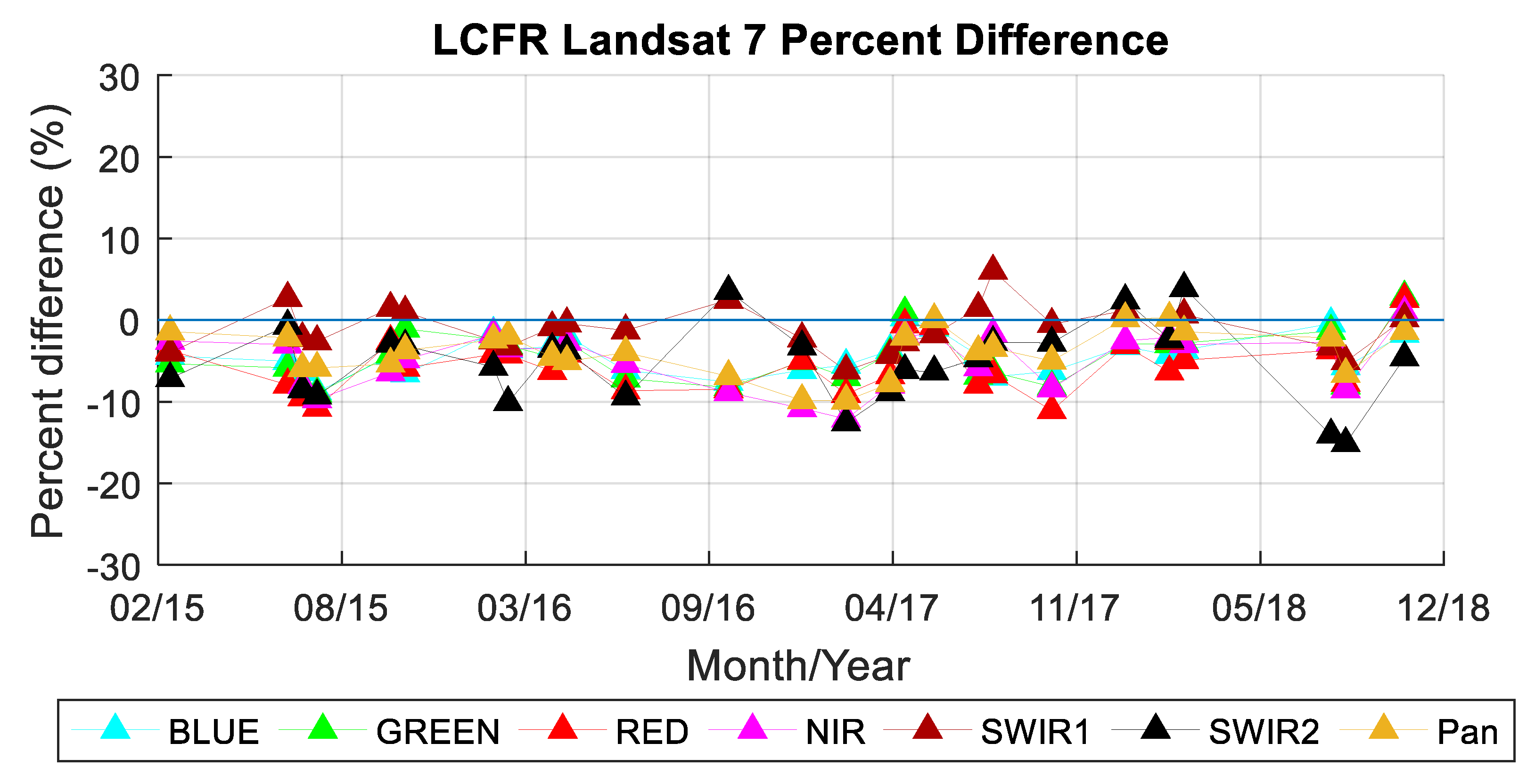
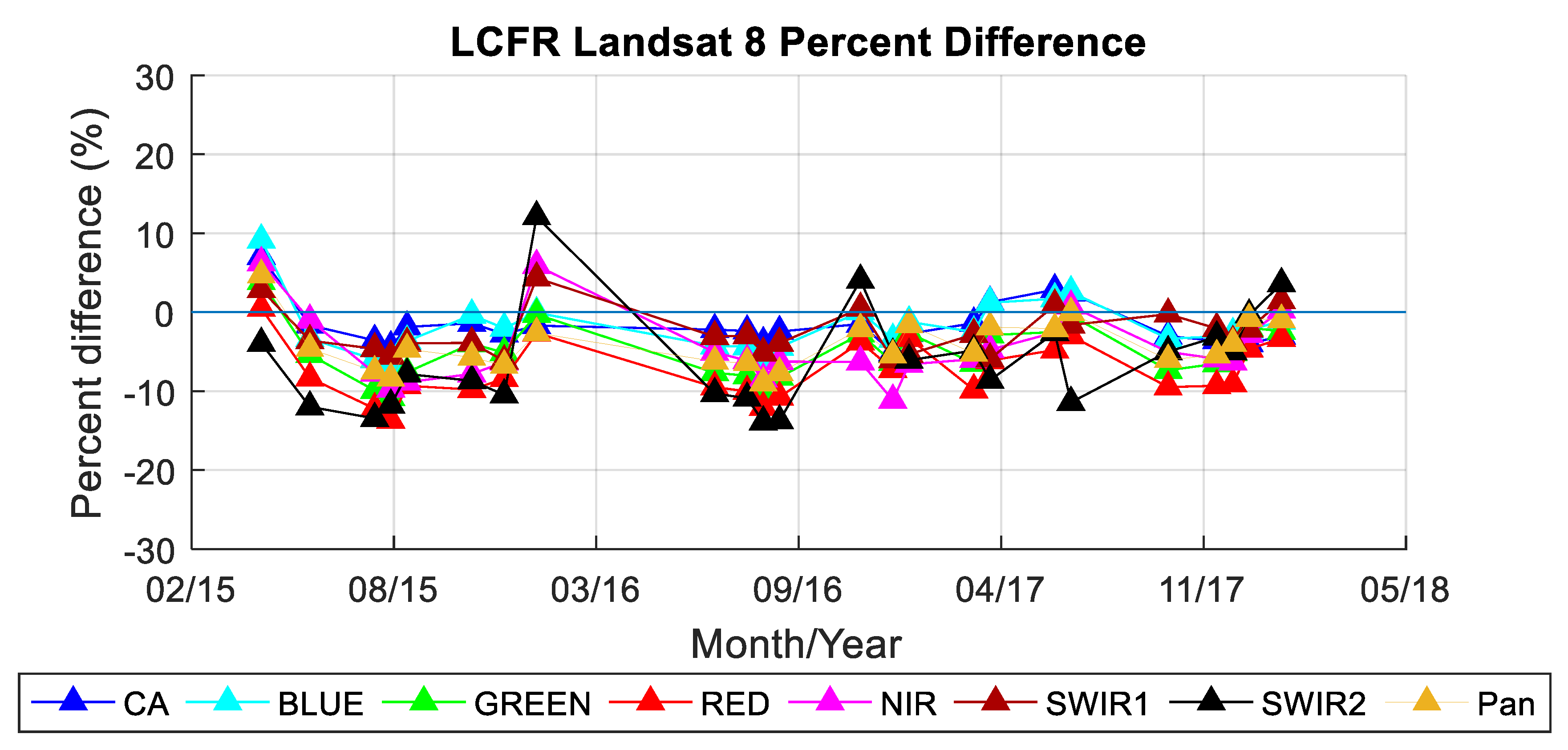
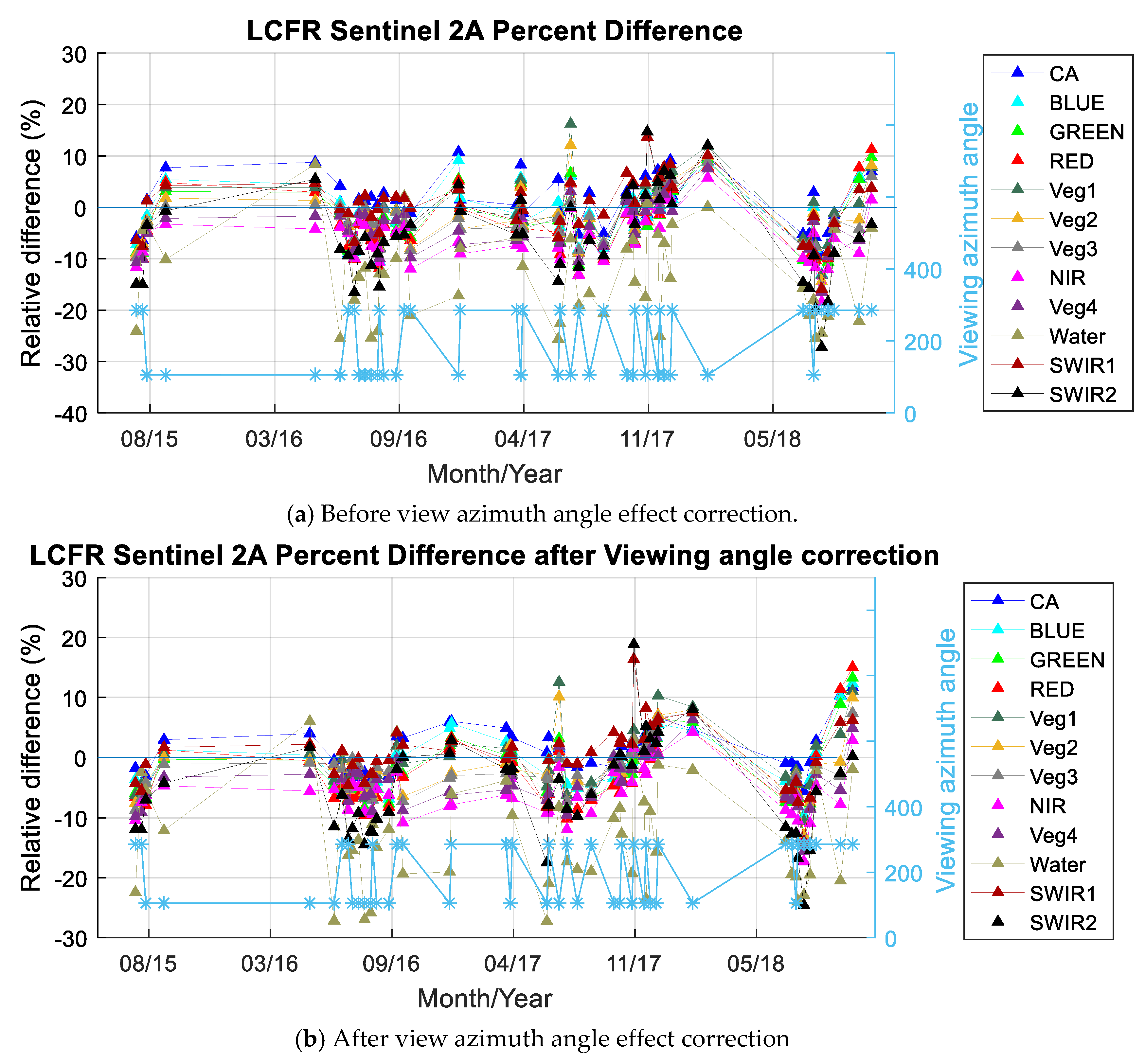
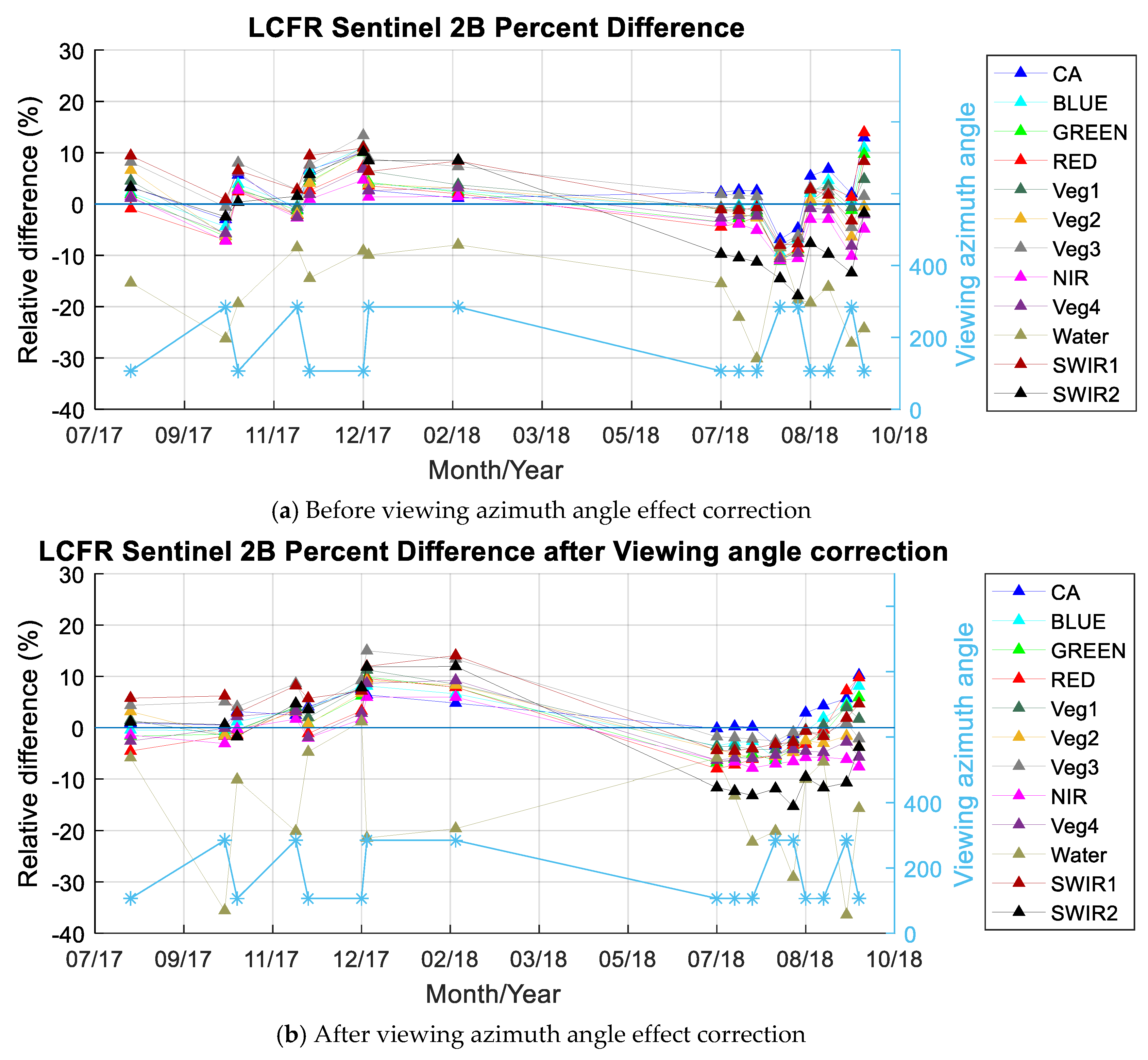
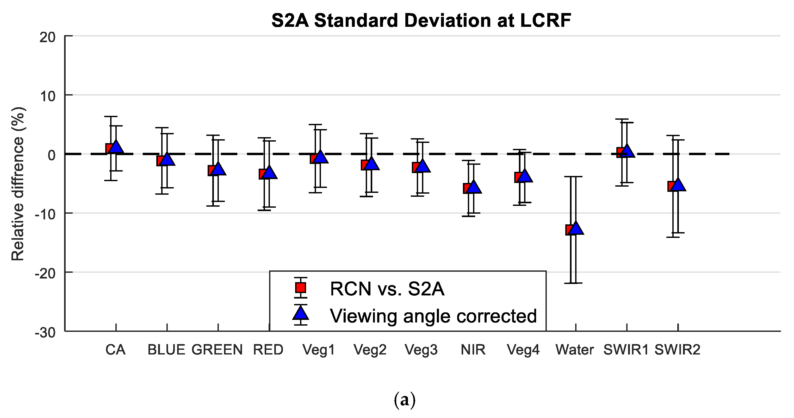
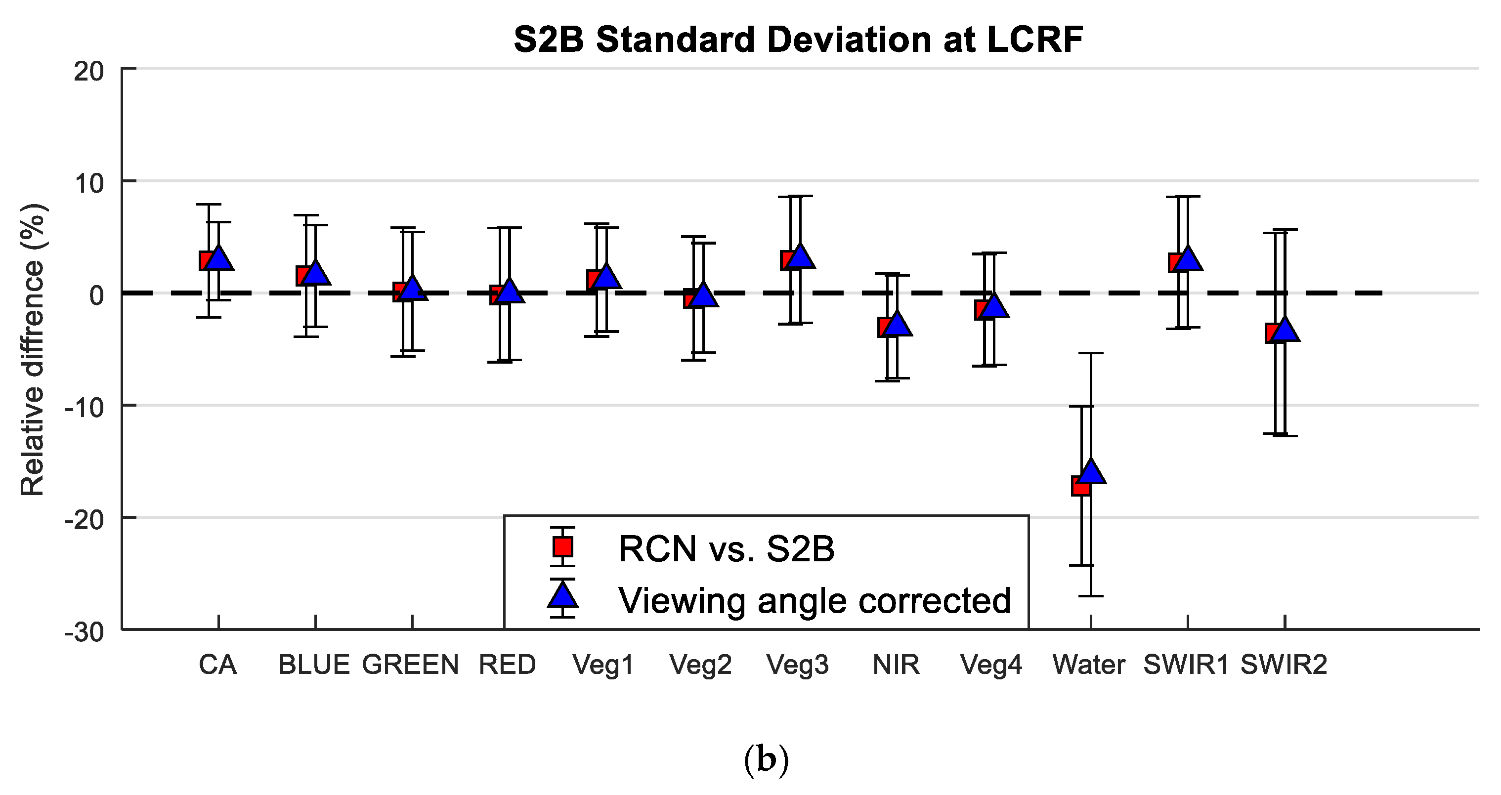
Figure 23 and Figure 24 show the temporal relative reflectance differences between LCFR RadCalNet predictions and the ETM+/OLI measurements, respectively. Figure 25 and Figure 26 show the relative TOA reflectance difference between the MSI sensors and RadCalNet before and after viewing angle effect correction, respectively. Figure 27 shows the corresponding mean and standard deviation values. The fluctuation of relative difference with respect to MSI viewing azimuth angle is generally reduced after application of the viewing angle effect correction. As with the RVUS results, the viewing angle effect correction preserves the mean relative difference. At LCFR, the correction reduces the scatter by approximately 0.5% for most bands except both water bands and the S2B MSI SWIR 2 band.

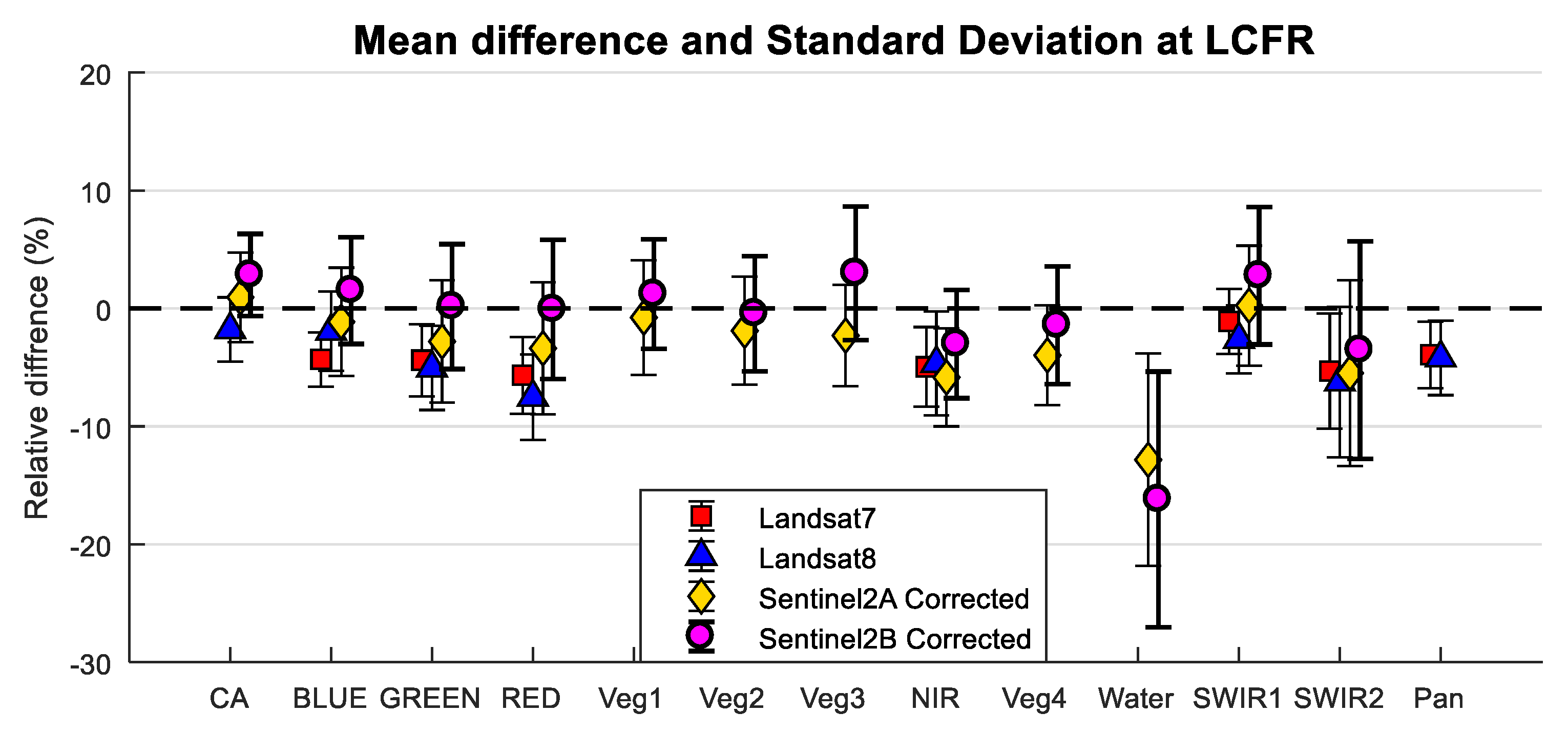
Figure 28 shows the relative TOA reflectance differences at LCFR between ETM+, OLI, and both MSIs after application of the viewing angle effect correction.

Table 3. Number of overpass dates, mean relative reflectance difference, and standard deviation for each sensor, LCFR.

Diff% ± Standard Deviation%
	ETM+	OLI	S2A MSI After Viewing Angle Effect Correction	S2B MSI After Viewing Angle Effect Correction
# of Overpasses	26	24	48	17
CA	N/A	−1.8 ± 2.7	0.9 ± 3.8	2.8 ± 3.5
Blue	−4.3 ± 2.3	−1.9 ± 3.4	−1.1 ± 4.6	1.5 ± 4.5
Green	−4.4 ± 3.1	−5.0 ± 3.6	−2.8 ± 5.2	0.2 ± 5.3
Red	−5.7 ± 3.3	−7.5 ± 3.6	−3.4 ± 5.6	−0.1 ± 5.9
Veg1	N/A	N/A	−0.8 ± 4.9	1.2 ± 4.6
Veg2	N/A	N/A	−1.9 ± 4.6	−0.4 ± 4.9
Veg3	N/A	N/A	−2.3 ± 4.3	3.0 ± 5.7
NIR	−5.0 ± 3.4	−4.7 ± 4.4	−5.8 ± 4.2	−3.0 ± 4.6
Veg4	N/A	N/A	−4.0 ± 4.2	−1.4 ± 5.0
Water	N/A	N/A	−12.8 ± 9.0	−16.2 ± 10.8
SWIR 1	−1.1 ± 2.7	−2.6 ± 2.9	0.2 ± 5.1	2.8 ± 5.8
SWIR 2	−5.3 ± 4.9	−6.2 ± 6.4	−5.5 ± 7.9	−3.5 ± 9.2
Pan	−3.9 ± 2.8	−4.2 ± 3.2	N/A	N/A

gives the number of overpasses and band-specific TOA reflectance difference means and standard deviations. As mentioned above, the value of standard deviation for all MSI bands is reduced by approximately 0.5% after the viewing angle effect correction; however, they are still approximately 1% greater than the corresponding ETM+ and OLI standard deviations. The mean relative difference of all ETM+, OLI, and 2A MSI bands are between approximately −10% and 1%; except the MSI water band, which is −12.8% ± 9.0%. The corresponding differences for S2B MSI bands are approximately within −3.5% to 3%; the water band difference is significantly greater, approximately −16.2% ± 10.8%.

4.3. Comparison of GONA Results

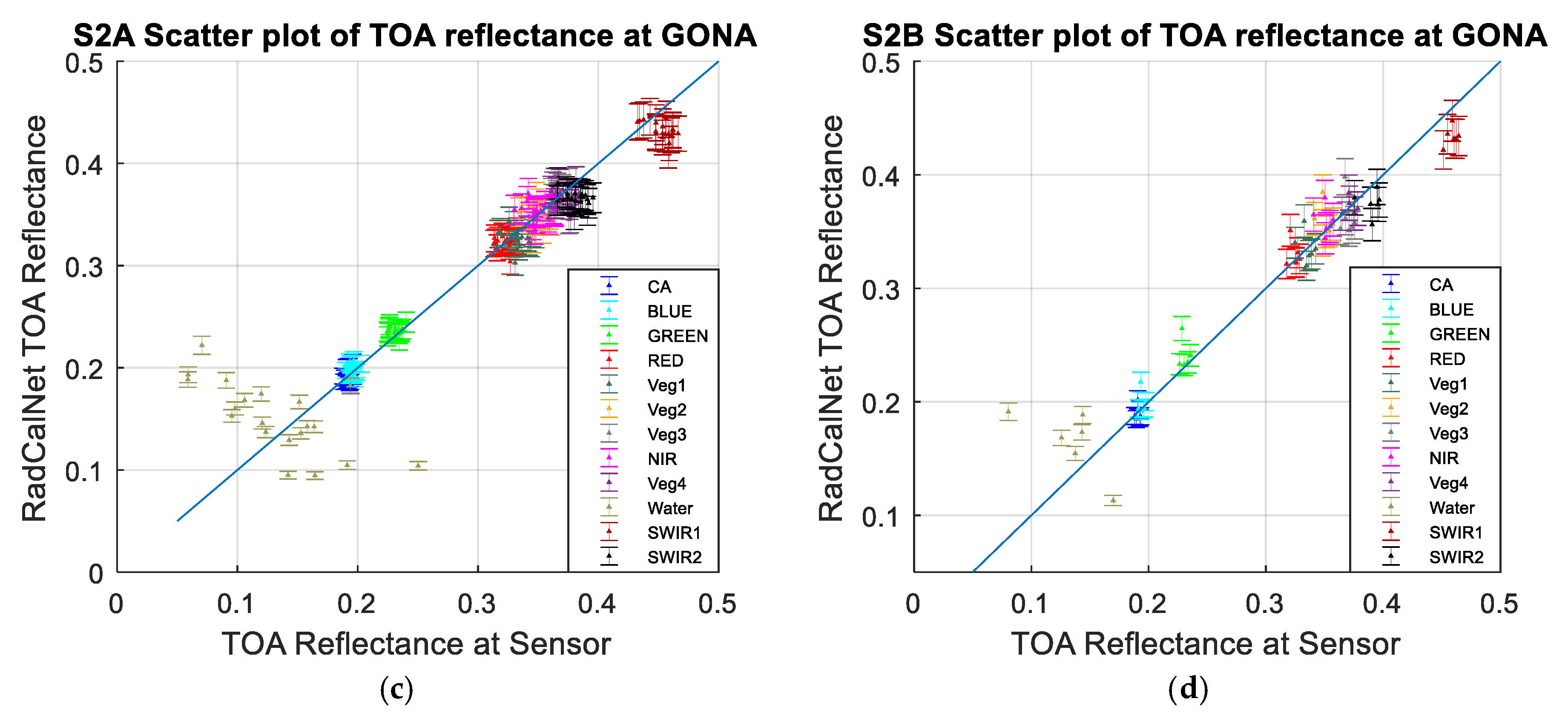
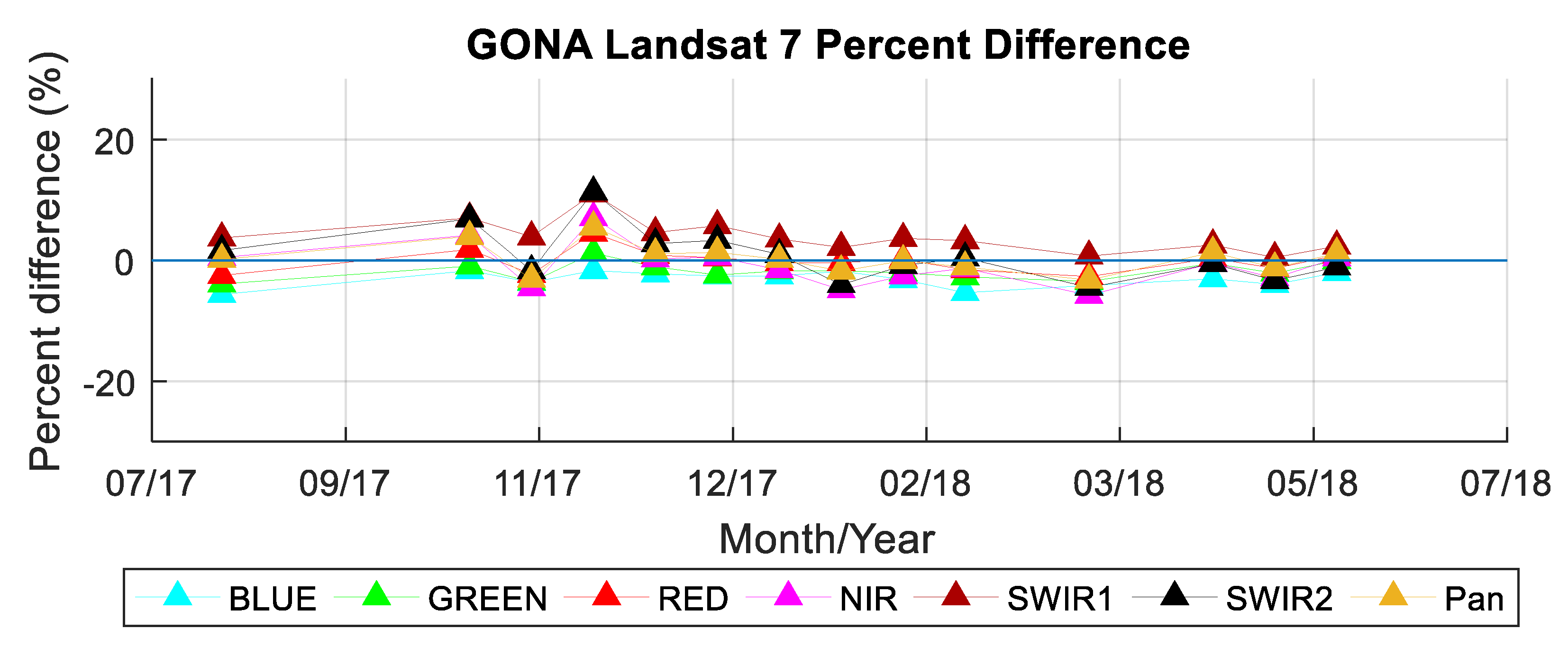
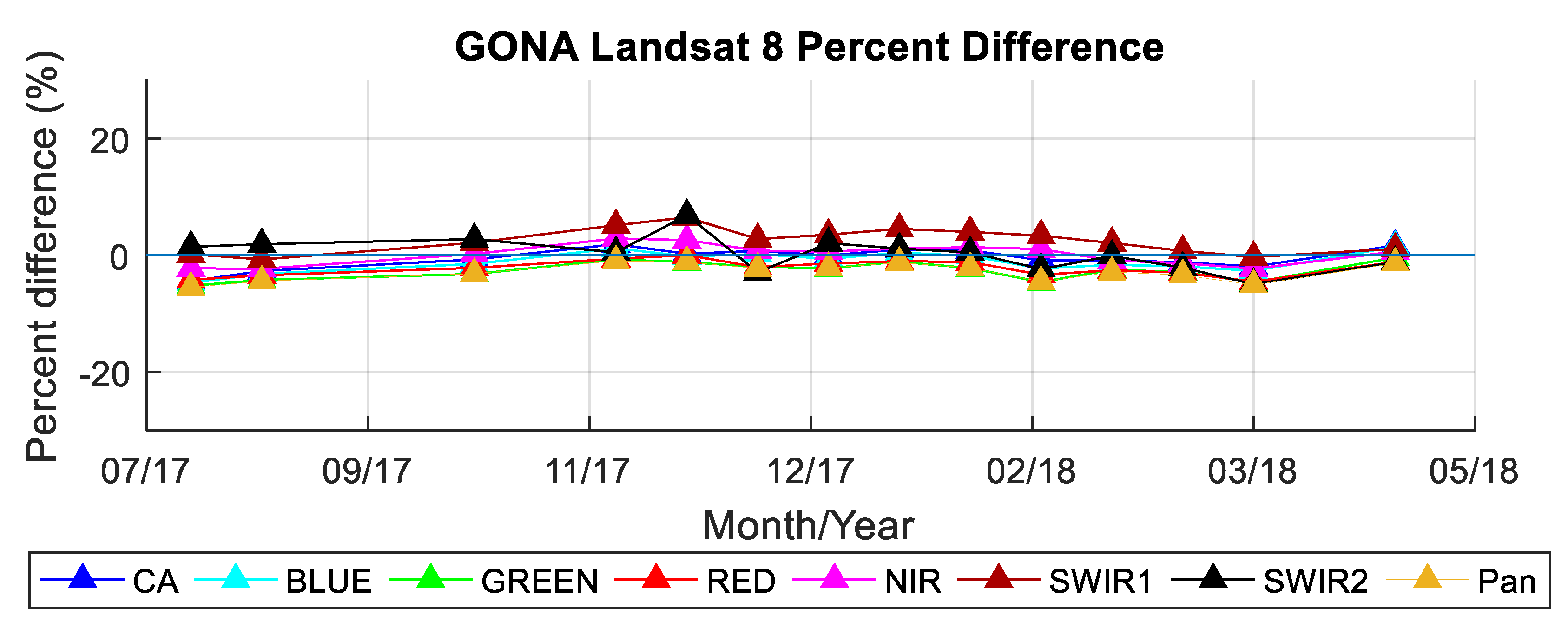
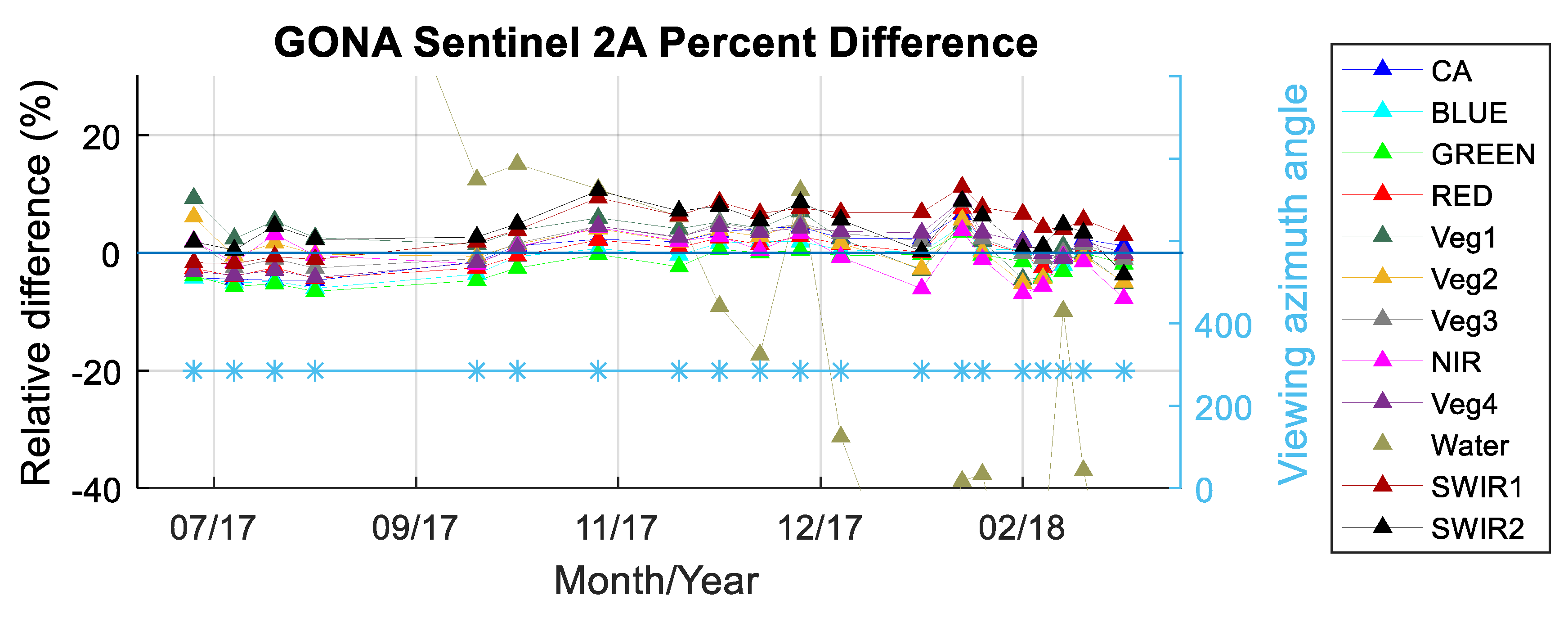
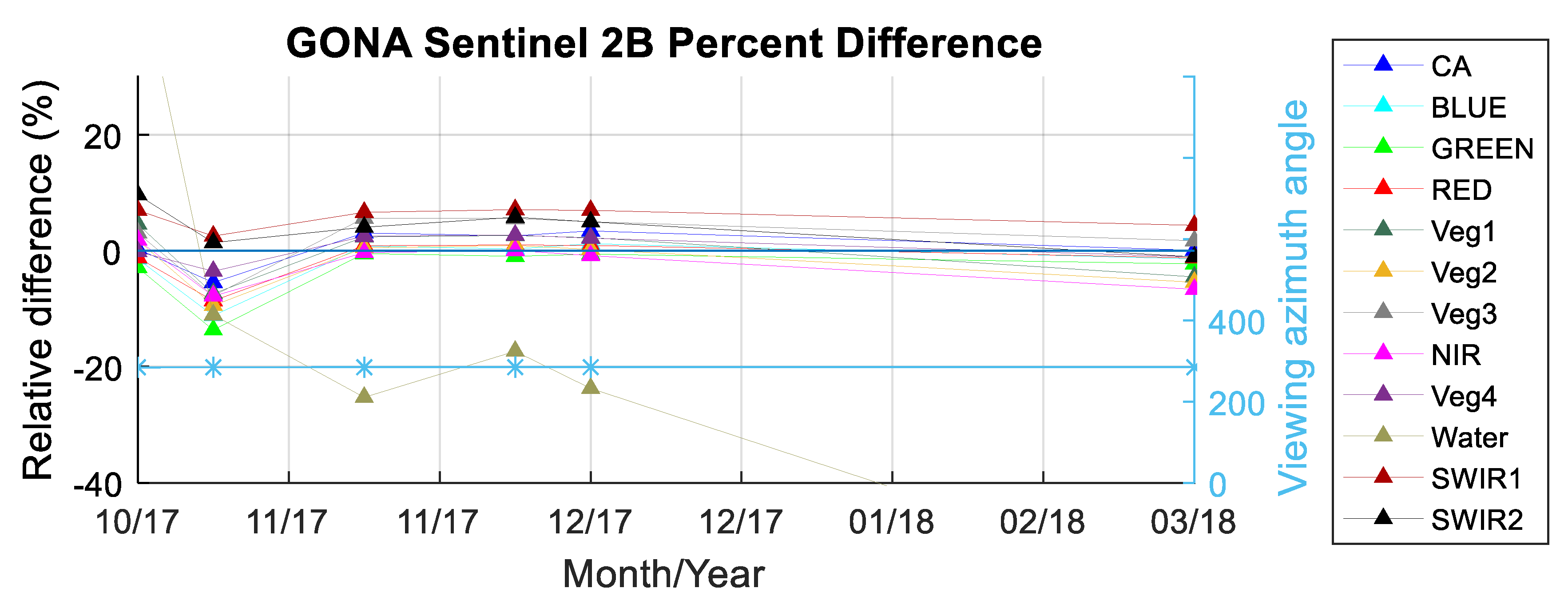
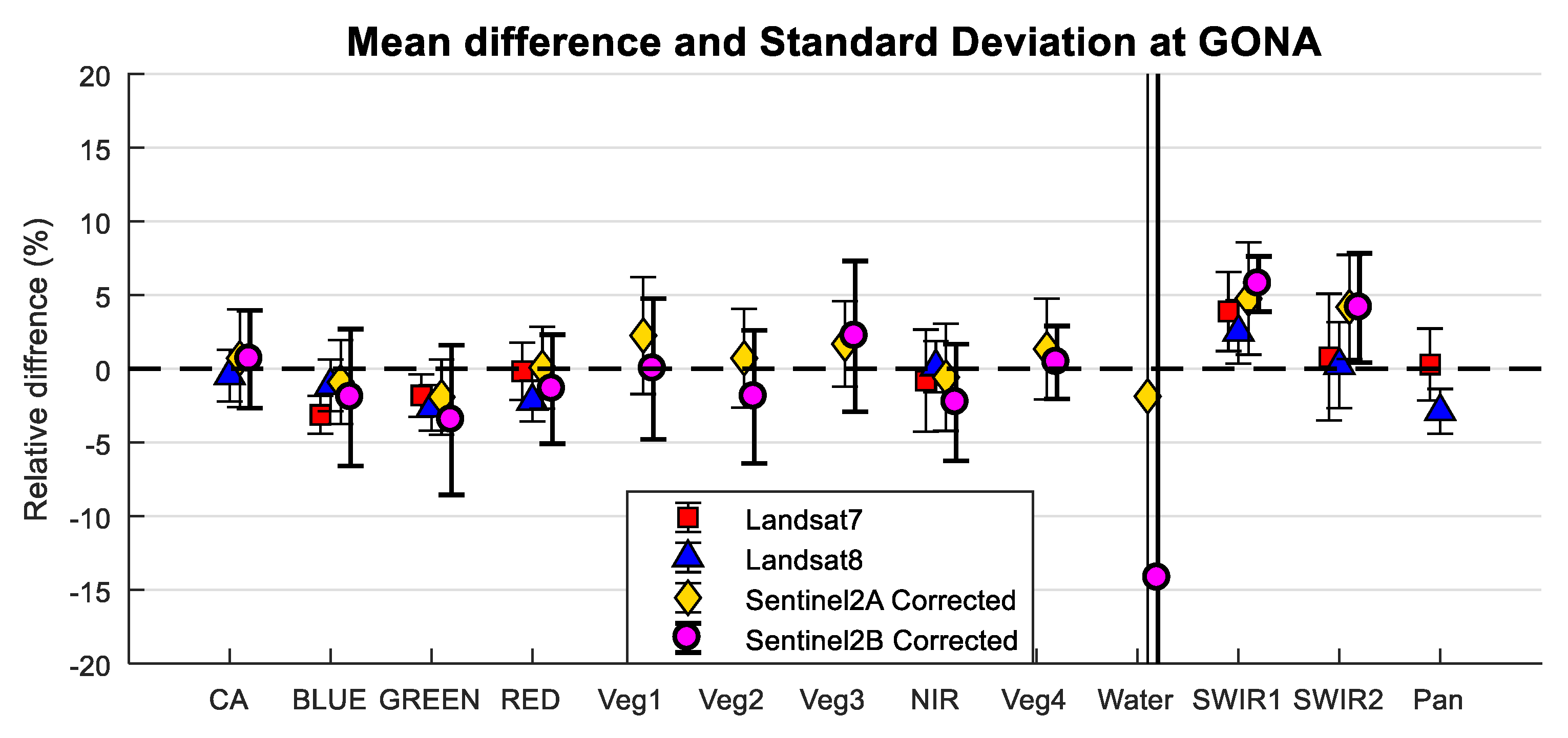
A major difference between GONA and the other sites studied in this work is that it is not located in adjacent swaths for the MSI sensors, and as a result a viewing angle effect correction is not needed. Performing the same comparisons as for the previous sites, the scatterplots and the temporal results for each sensor are shown in Figure 29a–d and Figure 30, Figure 31, Figure 32 and Figure 33, respectively. The average results are shown in Figure 34 and

Table 4. The number of overpass cases, mean, and standard deviation of TOA relative reflectance difference between three sensors and GONA site of all bands.

Diff% ± Standard Deviation%
	ETM+	OLI	S2A MSI After Viewing Angle Effect Correction	S2B MSI After Viewing angle Effect Correction
# of case	14	14	20	6
CA	N/A	−0.5 ± 1.7	0.7 ± 3.3	0.7 ± 3.3
Blue	−3.1 ± 1.3	−1.1 ± 1.8	−0.9 ± 2.8	−1.9 ± 4.6
Green	−1.8 ± 1.4	−2.7 ± 1.6	−1.9 ± 2.6	−3.5 ± 5.1
Red	−0.2 ± 1.9	−2.2 ± 1.4	0.1 ± 2.8	−1.4 ± 3.7
Veg1	N/A	N/A	2.3 ± 4.0	−0.0 ± 4.8
Veg2	N/A	N/A	0.7 ± 3.4	−1.9 ± 4.5
Veg3	N/A	N/A	1.7 ± 2.9	2.2 ± 5.1
NIR	−0.8 ± 3.5	0.2 ± 1.7	−0.6 ± 3.6	−2.3 ± 4.0
Veg4	N/A	N/A	1.3 ± 3.4	0.4 ± 2.5
Water	N/A	N/A	−1.9 ± 55.1	−14.2 ± 35.5
SWIR 1	3.9 ± 2.7	2.5 ± 2.1	4.8 ± 3.8	5.8 ± 1.9
SWIR 2	0.8 ± 4.3	0.2 ± 2.9	4.2 ± 3.5	4.1 ± 3.7
Pan	0.3 ± 2.4	−2.9 ± 1.5	N/A	N/A

.

It can be seen from Figure 29 that the data points for each sensor are more concentrated at GNBA than at the other sites in all bands except the MSI water bands, where the data points are extremely scattered. The authors of this paper reviewed the estimated water vapor content from each overpass, and found them similar to the values at RVUS. Consequently, an explanation for the observed scatter is yet unknown. On the other hand, the reasons for the overall concentration at GONA may be due to fewer data points, no overlap region for the MSI sensors, and less variation in the sensor-measured TOA reflectances shown in Figure 8 and Figure 9.

For the studied sensors, this site is much more consistent with respect to the mean relative TOA reflectance difference and standard deviation. It should be noted this site began active operation on 2017-07-19, and thus has much fewer coincident overpasses than RVUS and LCFR (Table 4).

The trends of average relative reflectance difference as a function of band in each sensor shown in Figure 34 are similar, and are generally within ±5% in all bands except the S2B MSI water band, which is within approximately ±20%. These results are consistent with the corresponding RVUS results for ETM+, OLI and S2A MSI. Note that as shown in Figure 8, data from the 2300 nm to 2500 nm spectral region was removed. As this region lies within parts of the SWIR 2 bands in ETM+, OLI, and S2A MSI, an additional uncertainty will be introduced when calculating the relative difference, even though the mean relative difference in the SWIR 2 band of each sensor is within approximately 4.2%. Another factor to consider is that at GONA, the relative mean differences of S2B MSI are consistent with the other sensors. This intersensor difference is most likely due to the one viewing azimuth direction used at this site, which changes the relative mean difference and reduces the data scatter.

5. Conclusions

This work focuses on the performance comparison of the acquired surface measurements at the RVUS, LCFR, and GONA RadCalNet sites using ETM+, OLI, and S2A/S2B MSI sensors. It has identified a significant viewing angle effect at RVUS and LCFR that affects the MSIs; this effect manifests as differences in azimuth angle between overlapping swaths from adjacent orbits, and is caused by BRDF effects due to the view angle. A correction has been developed and applied to the MSI data; the resulting standard deviations in TOA reflectance between RadCalNet and S2A/S2B MSIs were reduced by approximately 2% and 0.5%, respectively.

With application of the viewing angle effect correction to the MSI data, the average relative reflectance differences at RVUS and GONA are consistently within ± 5% in all bands except the S2A MSI water band and S2B MSI bands at RVUS, which are generally within a range of 7% to 13%. These two sites, overall, provide comparable results among each of the studied sensors. The large differences observed in S2B MSI at RVUS need to be further investigated, however.

The average relative reflectance differences observed at LCFR are different from those at RVUS and GONA in general. For ETM+, OLI, and S2A MSI, the average relative reflectance difference of all bands in each sensor is between approximately −10% and 1%. However, except the water band, the corresponding S2B MSI average relative reflectance differences are within −3.5% and 3%, which is consistently higher than other sensors. Some of this difference may be explained by the fact there are less data.

An automated RadCalNet concept has been under consideration and development by the CEOS IVOS WG for several years, and has demonstrated significant potential for use in sensor radiometric calibration. The data from RadCalNet are easy to acquire and use. Considering the results shown in this work, more effort is needed to better understand the behavior at LCFR, above and beyond the obvious difference that it is a vegetative site. At this time, perhaps the most significant limitation on the accuracy of the RadCalNet data is the development of an appropriate site-specific BRDF characterization and correction.

References

- Wenny, B.; Bouvet, M.; Thome, K.J.; Czapla-Myers, J.S.; Fox, N.; Gory, P.; Henry, P.; Meygret, A.; Li, C.; Ma, L.; et al. RadCalNet: A prototype radiometric calibration network for Earth observing imagers. In Proceedings of the Joint Agency Commercial Imagery Evaluation (JACIE) Workshop, Fort Worth, TX, USA, 12–14 April 2016. [Google Scholar]
- RadCalNet Technical Working Group. RadCalNet Guidance: Instrumentation and Data Processing (QA4EO-WGCV-RadCalNet-G3_v1); Committee on Earth Observation Satellites, 2018. Available online: https://www.radcalnet.org/documentation/RadCalNetGenDoc/G3-RadCalNetGuidance-InstrumentationAndDataProcessing_V1.pdf (accessed on 5 March 2019).
- Czapla-Myers, J.S.; Thome, K.J.; Leisso, N.P. Radiometric calibration of earth-observing sensors using an automated test site at Railroad Valley, Nevada. Can. J. Remote Sens. 2010, 36, 474–487. [Google Scholar] [CrossRef]
- University of Arizona. RadCalNet Site Description (QA4EO-WGCV-IVO-CSP-002_RVUS); Committee on Earth Observation Satellites: Railroad Valley, NV, USA, 2016. [Google Scholar]
- Czapla-Myers, J.; McCorkel, J.; Anderson, N.; Thome, K.; Biggar, S.; Helder, D.; Mishra, N. The ground-based absolute radiometric calibration of Landsat 8 OLI. Remote Sens. 2015, 7, 600–626. [Google Scholar] [CrossRef]
- CNES Physics for Optical Measurement Department. RadCalNet Site Description (QA4EO-WGCV-IVO-CSP-002_LCFR); Committee on Earth Observation Satellites: La Crau, France, 2016. [Google Scholar]
- National Physical Laboratory. RadCalNet Site Description (QA4EO-WGCV-IVO-CSP-002_GONA); Committee on Earth Observation Satellites: Gobabeb, Namibia, 2016. [Google Scholar]
- Zanter, K. Landsat 8 (L8) Data Users Handbook. Landsat Science Official Website. 2016. Available online: https://landsat.usgs.gov/landsat-8-l8-data-users-handbook (accessed on 20 January 2018).
- Gatti, A.; Bertolini, A. Sentinel-2 Products Specification Document. 2013. Available online: https://earth.esa.int/documents/247904/685211/Sentinel-2+Products+Specification+Document (accessed on 23 February 2015).
- Kaewmanee, M. Pseudo Invariant Calibration Sites: PICS Evolution. In Proceedings of the Conference on Characterization and Radiometric Calibration for Remote Sensing (CALCON), Logan, UT, USA, 18–20 June 2018. [Google Scholar]
- Chander, G.; Markham, B.L.; Helder, D.L. Summary of current radiometric calibration coefficients for Landsat MSS, TM, ETM+, and EO-1 ALI sensors. Remote Sens. Environ. 2009, 113, 893–903. [Google Scholar] [CrossRef] [Green Version]
- Mishra, N.; Haque, M.O.; Leigh, L.; Aaron, D.; Helder, D.; Markham, B. Radiometric cross calibration of Landsat 8 operational land imager (OLI) and Landsat 7 enhanced thematic mapper plus (ETM+). Remote Sens. 2014, 6, 12619–12638. [Google Scholar] [CrossRef]
- Czapla-Myers, J.; McCorkel, J.; Anderson, N.; Biggar, S. Earth-observing satellite intercomparison using the Radiometric Calibration Test Site at Railroad Valley. J. Appl. Remote Sens. 2017, 12, 012004. [Google Scholar] [CrossRef]
- Pinto, C.T.; Ponzoni, F.J.; Castro, R.M.; Leigh, L.; Kaewmanee, M.; Aaron, D.; Helder, D. Evaluation of the uncertainty in the spectral band adjustment factor (SBAF) for cross-calibration using Monte Carlo simulation. Remote Sens. Lett. 2016, 7, 837–846. [Google Scholar] [CrossRef]
- Chander, G.; Helder, D.L.; Aaron, D.; Mishra, N.; Shrestha, A.K. Assessment of spectral, misregistration, and spatial uncertainties inherent in the cross-calibration study. IEEE Trans. Geosci. Remote Sens. 2013, 51, 1282–1296. [Google Scholar] [CrossRef]
Figure 1.
(a) A 2017-07-04 operational land imager (OLI) image of RVUS and its surface measurement region (yellow square). (b) The site view of Railroad Valley [3].
Figure 2.
(a) Measured surface reflectance acquired every 30 minutes between 09:00 and 15:00 local time at RVUS on 2015-07-15 and (b) the associated uncertainties.
Figure 3.
(a) RVUS top-of-atmosphere (TOA) reflectances derived from cloud-free ETM+ overpasses, 2013–2018 and (b) the associated uncertainties.
Figure 4.
(a) 2017-04-20 OLI image of LCFR and its surface measurement region (red square). (b) Typical LCFR surface cover at the beginning of summer [5].
Figure 5.
(a) Measured surface reflectance acquired every 30 minutes between 09:00 and 15:00 local time at LCFR on 2015-06-02 and (b) the associated uncertainties.
Figure 6.
(a) LCFR TOA reflectances derived from cloud-free ETM+ overpasses, 2015–2018; (b) the associated uncertainty.
Figure 7.
In (a) 2017-08-19 OLI image of GONA and its surface measurement region (yellow square); and in (b) Typical GONA surface cover [6].
Figure 8.
(a) Measured surface reflectance acquired every 30 minutes between 09:00 and 15:00 local time at GONA on 2017-08-08; (b) the associated uncertainties.
Figure 9.
(a) GONA TOA reflectances derived from cloud-free ETM+ overpasses, 2017–2018; (b) the associated uncertainty.
Figure 10.
Two S2A MSI images of RVUS acquired on (a) 2016-07-15 and (b) 2016-08-07, respectively. The arrows indicate the sensor viewing direction.
Figure 11.
Scatterplots of RVUS RadCalNet predicted and measured TOA reflectances for (a) ETM+, (b) OLI, (c) S2A MSI, and (d) S2B MSI.
Figure 12.
Relative reflectance difference between ETM+ and RadCalNet at RVUS.
Figure 13.
Relative reflectance difference between OLI and RadCalNet at RVUS.
Figure 14.
Relative reflectance difference between S2A MSI and RadCalNet at RVUS without viewing angle correction. The blue line with ‘*’ is the viewing azimuth angle.
Figure 15.
Relative reflectance difference between S2B MSI and RadCalNet at RVUS without viewing angle correction. The blue line with ‘*’ is the viewing azimuth angle.
Figure 16.
Sensor viewing and solar geometries at RVUS for (a) S2A and (b) S2B.
Figure 17.
Relative reflectance difference between S2A MSI and RadCalNet at RVUS after viewing azimuth angle effect correction.
Figure 18.
Relative reflectance difference between S2B MSI and RadCalNet at RVUS after viewing azimuth angle effect correction.
Figure 19.
The average relative reflectance difference of S2A MSI and RadCalNet before and after viewing angle effect correction.
Figure 20.
The average relative reflectance difference of S2B MSI and RadCalNet at RVUS before and after viewing angle effect correction.
Figure 21.
The average relative reflectance difference of Landsat 7, Landsat 8, and S2A/S2B MSI after viewing angle effect correction at RVUS.
Figure 22.
Scatterplots of LCFR RadCalNet predicted and measured TOA reflectances for (a) ETM+, (b) OLI, (c) S2A MSI, and (d) S2B MSI.
Figure 23.
Relative reflectance difference between ETM+ and RadCalNet at LCFR.
Figure 24.
Relative reflectance difference between OLI and RadCalNet at LCFR.
Figure 25.
Percent TOA reflectance difference between S2A MSI and RadCalNet at LCFR (a) before and (b) after viewing azimuth angle effect correction.
Figure 26.
Percent TOA reflectance difference between S2B MSI and RadCalNet at LCFR (a) before and (b) after viewing azimuth angle effect correction.
Figure 27.
The average relative reflectance difference of S2A (a) and S2B (b) before and after viewing angle effect correction on LCFR.
Figure 28.
The average relative reflectance difference of Landsat 7 and Landsat 8 before and after viewing angle effect correction of Sentinel 2A on LCFR.
Figure 29.
Scatterplots of GONA RadCalNet predicted and measured TOA reflectances for (a) ETM+, (b) OLI, (c) S2A MSI, and (d) S2B MSI.
Figure 30.
Relative reflectance difference between ETM+ and RadCalNet at GONA.
Figure 31.
Relative reflectance difference between OLI and RadCalNet at GONA.
Figure 32.
Relative reflectance difference between S2A MSI and RadCalNet at GONA.
Figure 33.
Relative reflectance difference between S2B MSI and RadCalNet at GONA.
Figure 34.
The average relative reflectance difference of the Landsat 7, Landsat 8, and Sentinel 2A view angle effect corrected on GONA.