Challenges and Best Practices for Deriving Temperature Data from an Uncalibrated UAV Thermal Infrared Camera

 , , , , ,
Abstract
:
1. Introduction
2. Materials and Methods
2.1. Laboratory Experiments
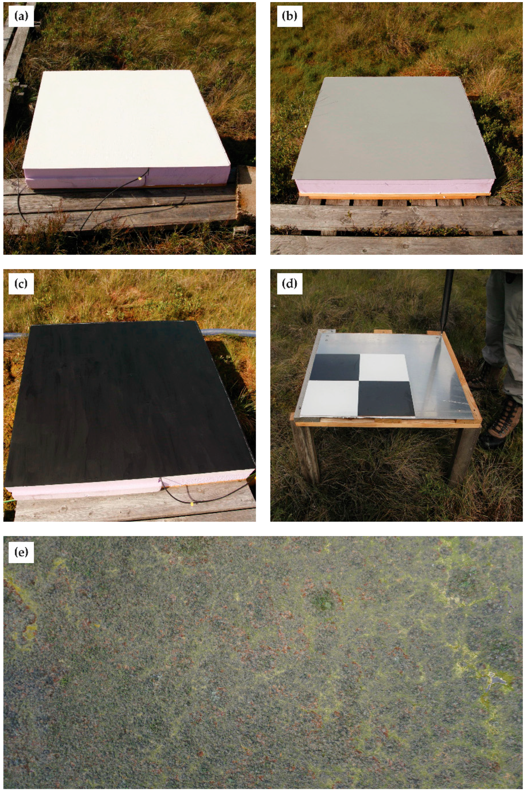
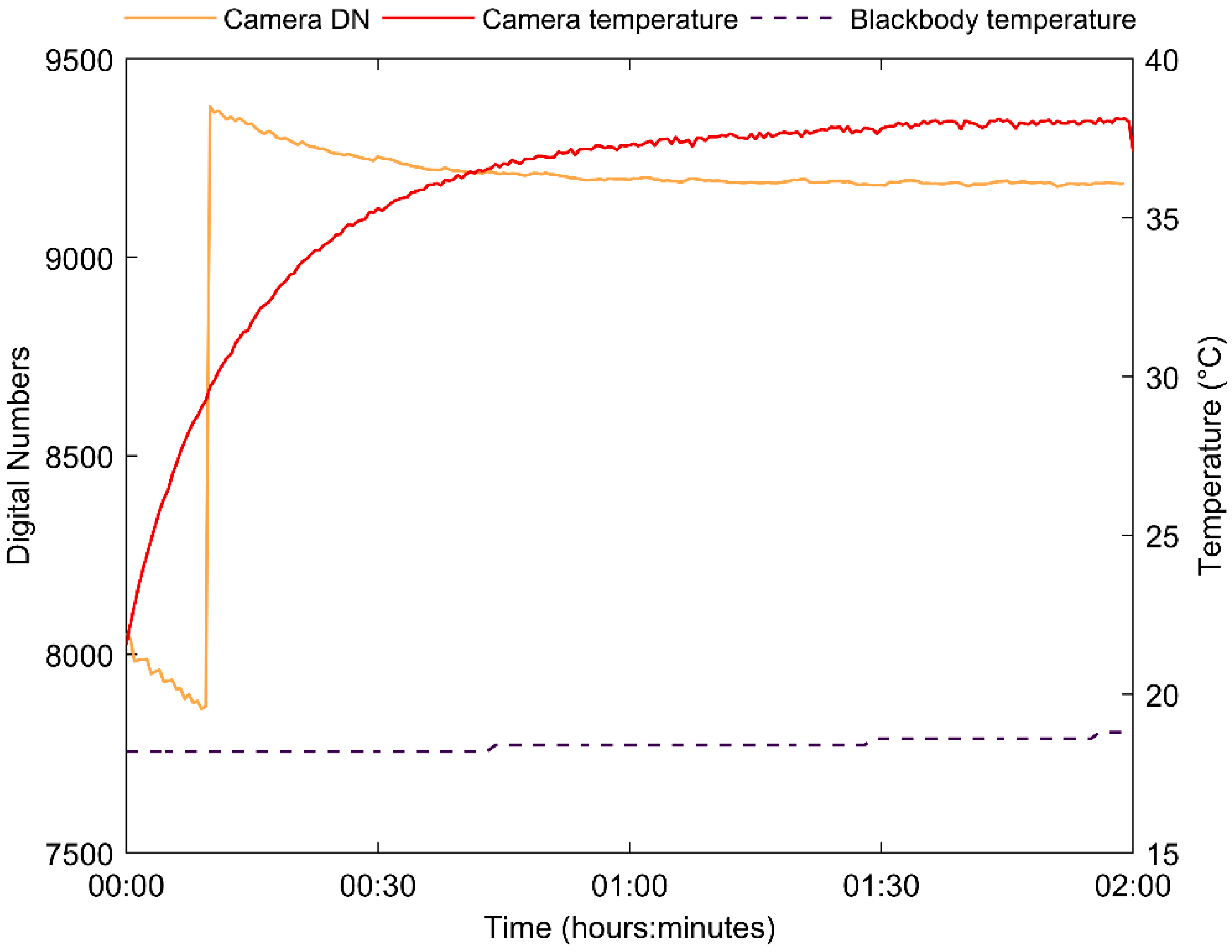
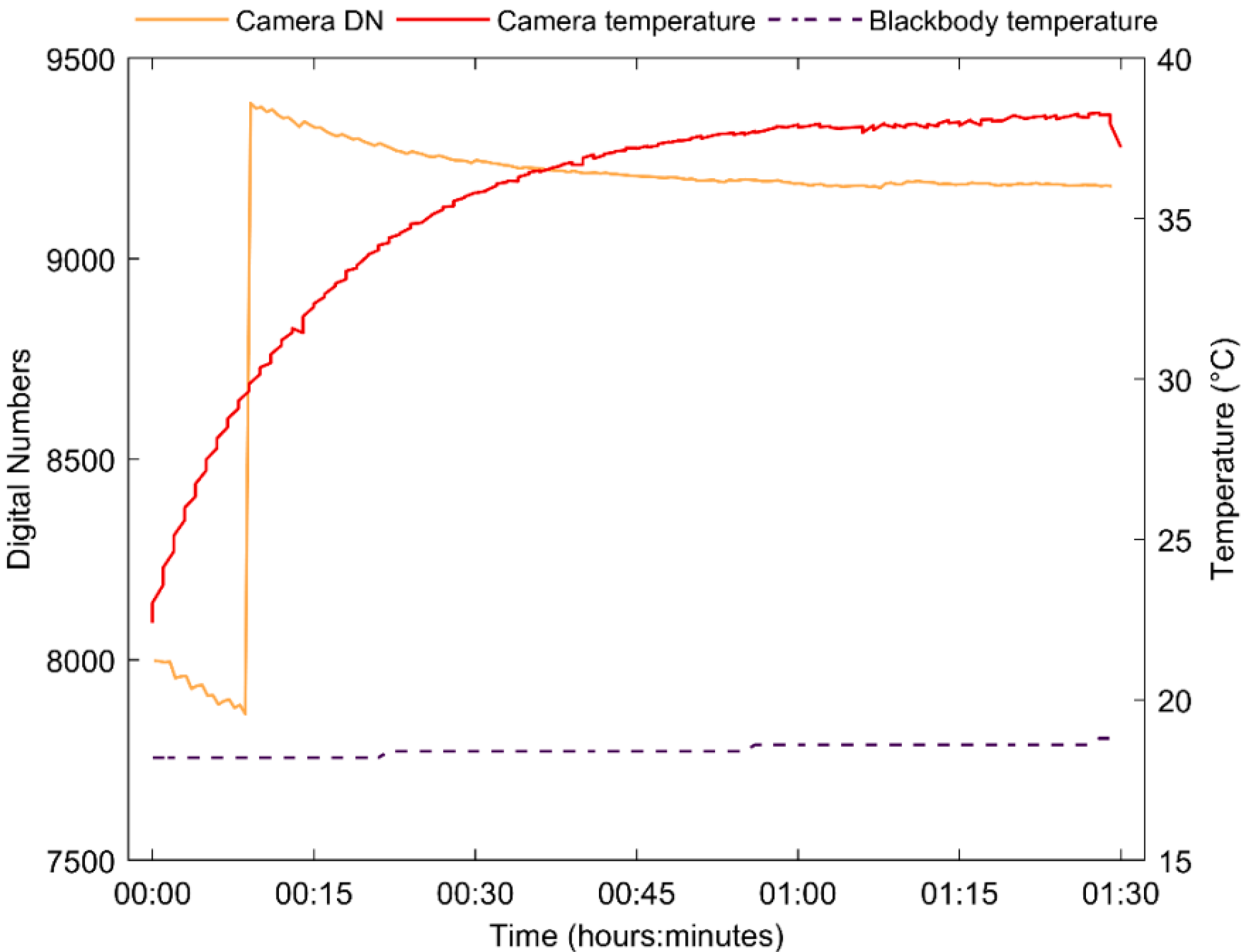
2.1.1. Stabilization Time and Blackbody Curves
2.1.2. Wind and Radiative Effects
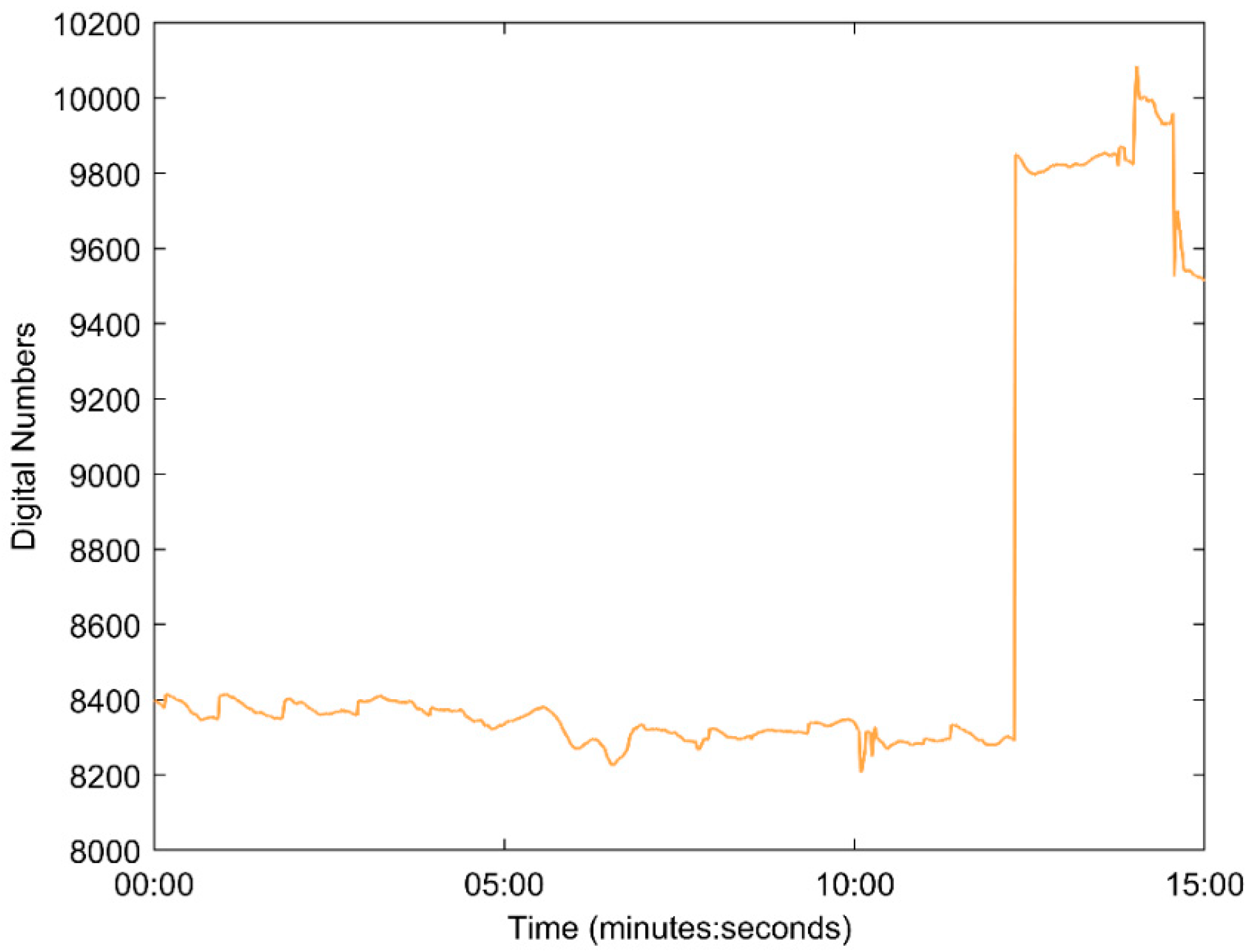
2.1.3. Sensor Noise
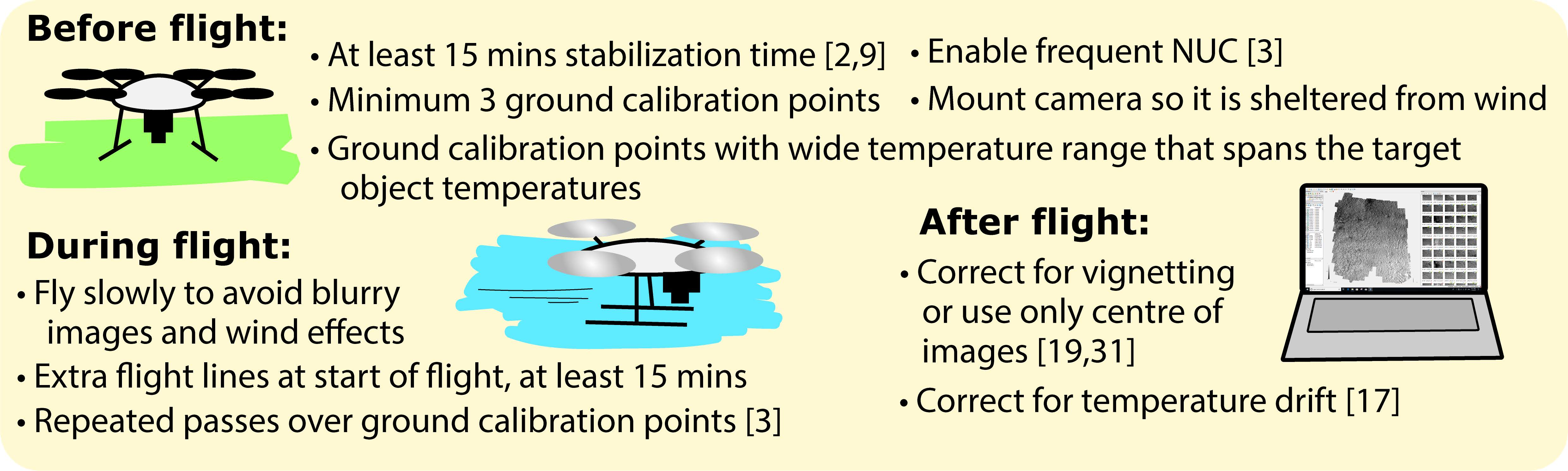
2.2. Field Calibration and Validation
2.2.1. Radiometric Calibration
2.2.2. Orthomosaic Creation
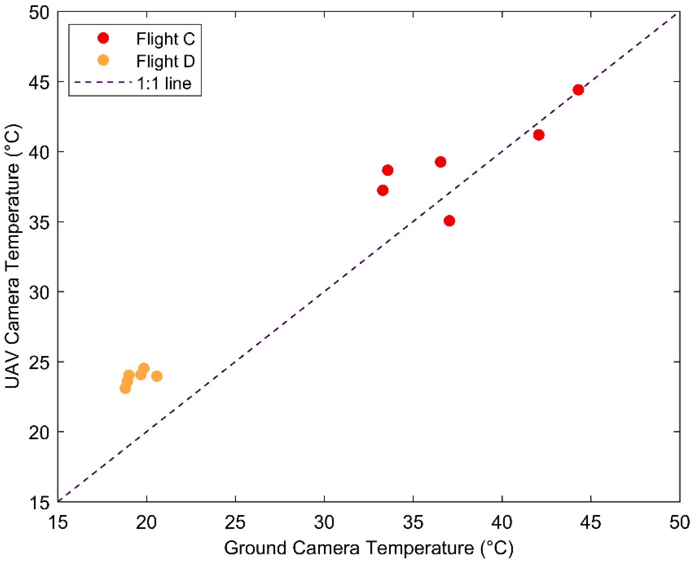
2.2.3. Validation
3. Results
3.1. Laboratory Experiments
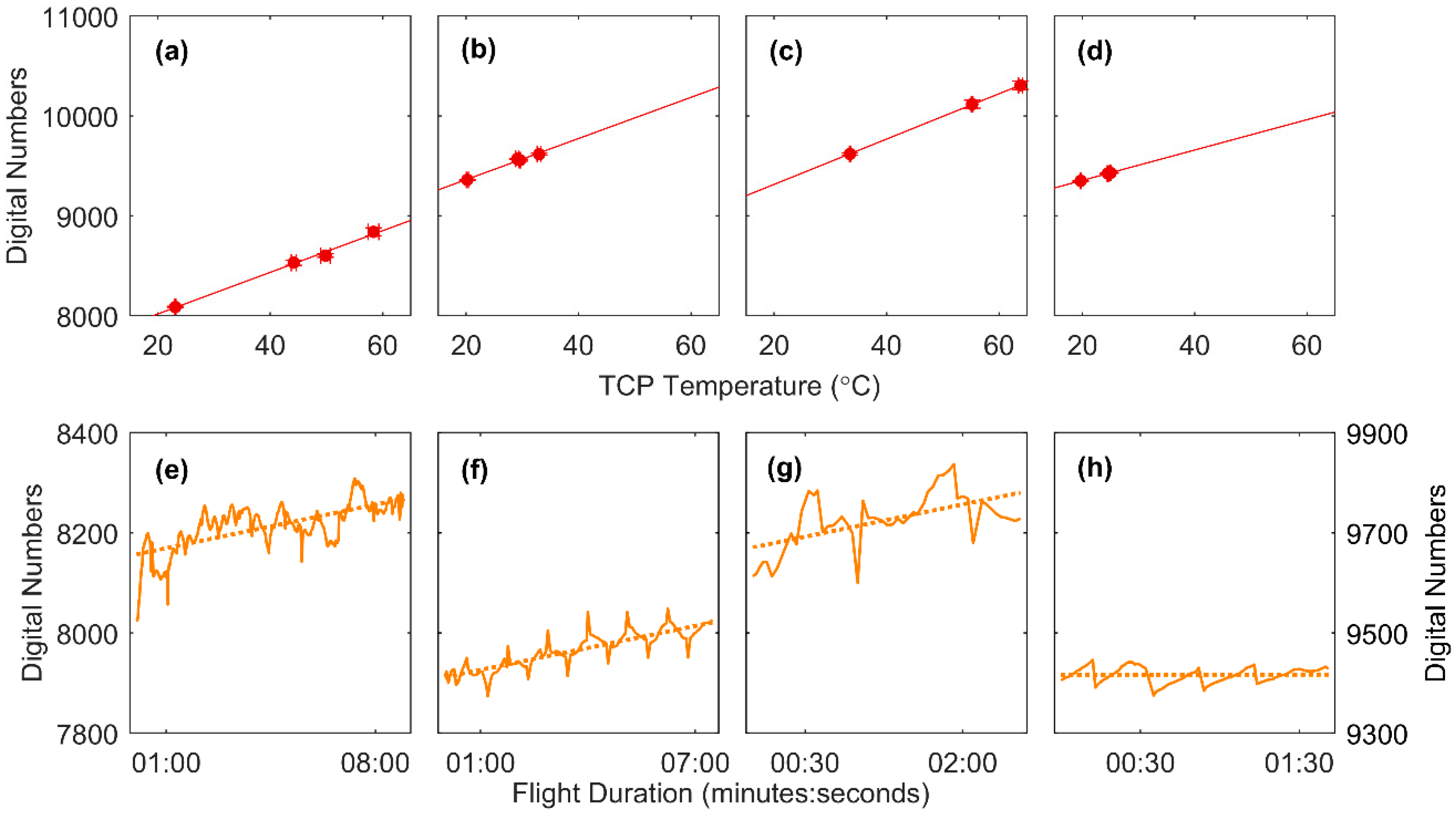
3.1.1. Stabilization Time
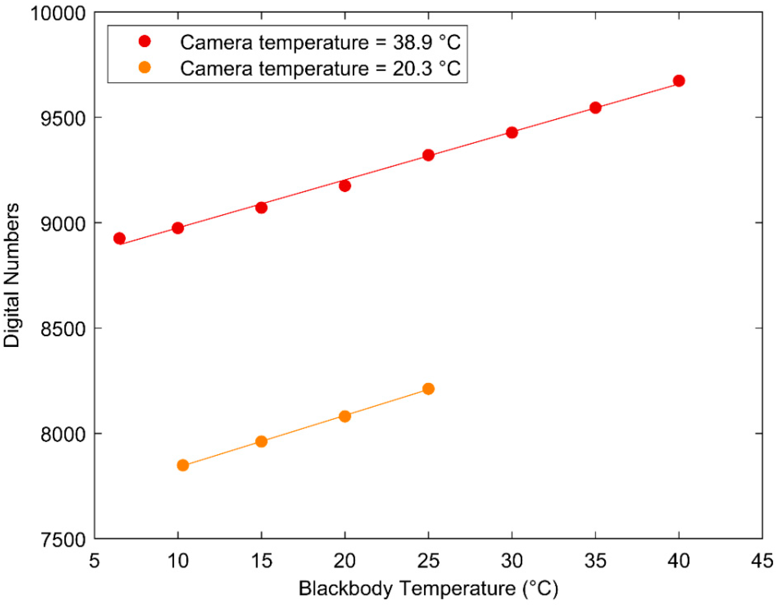
3.1.2. Blackbody Curves
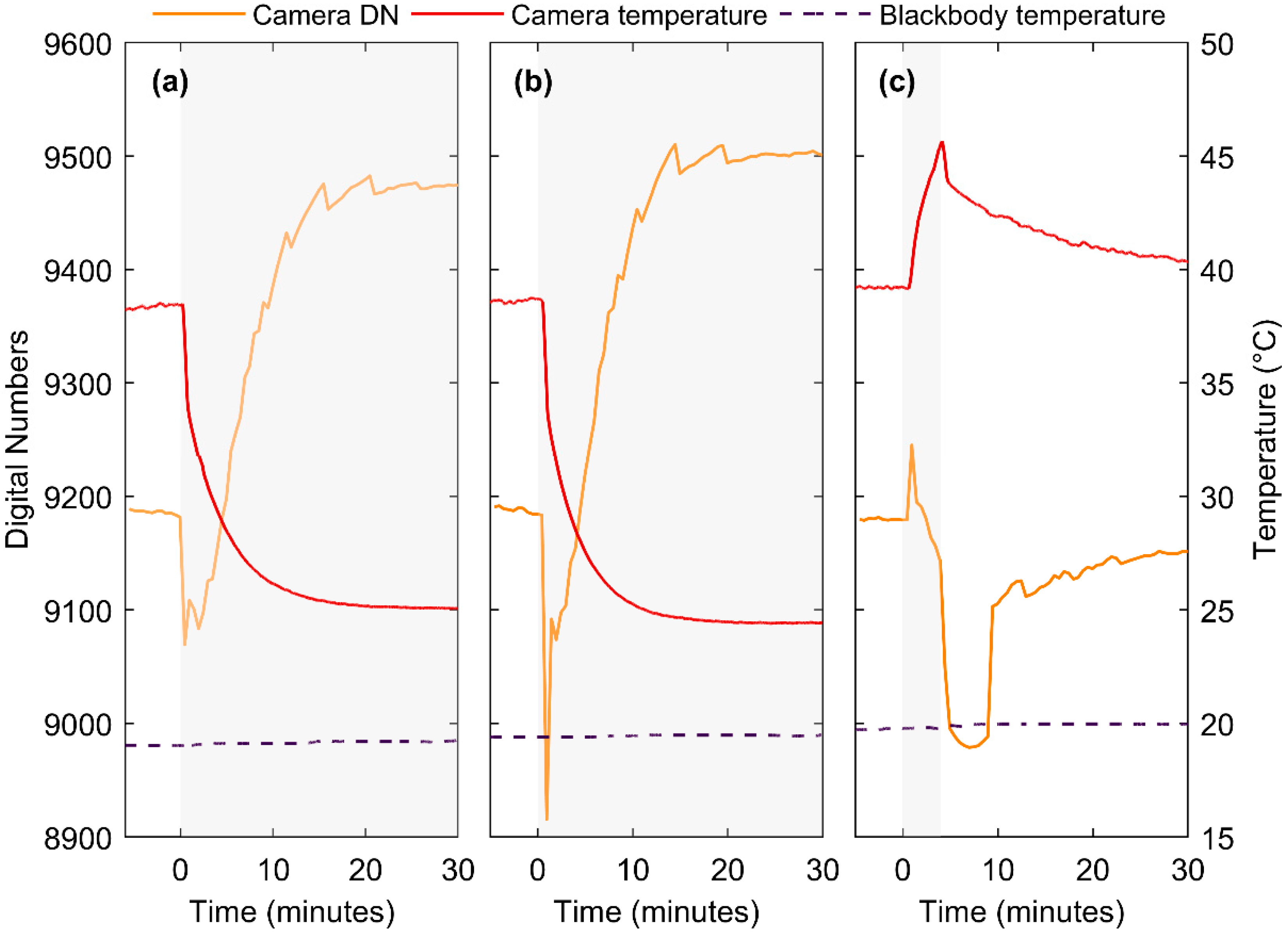
3.1.3. Wind and Radiative Effects
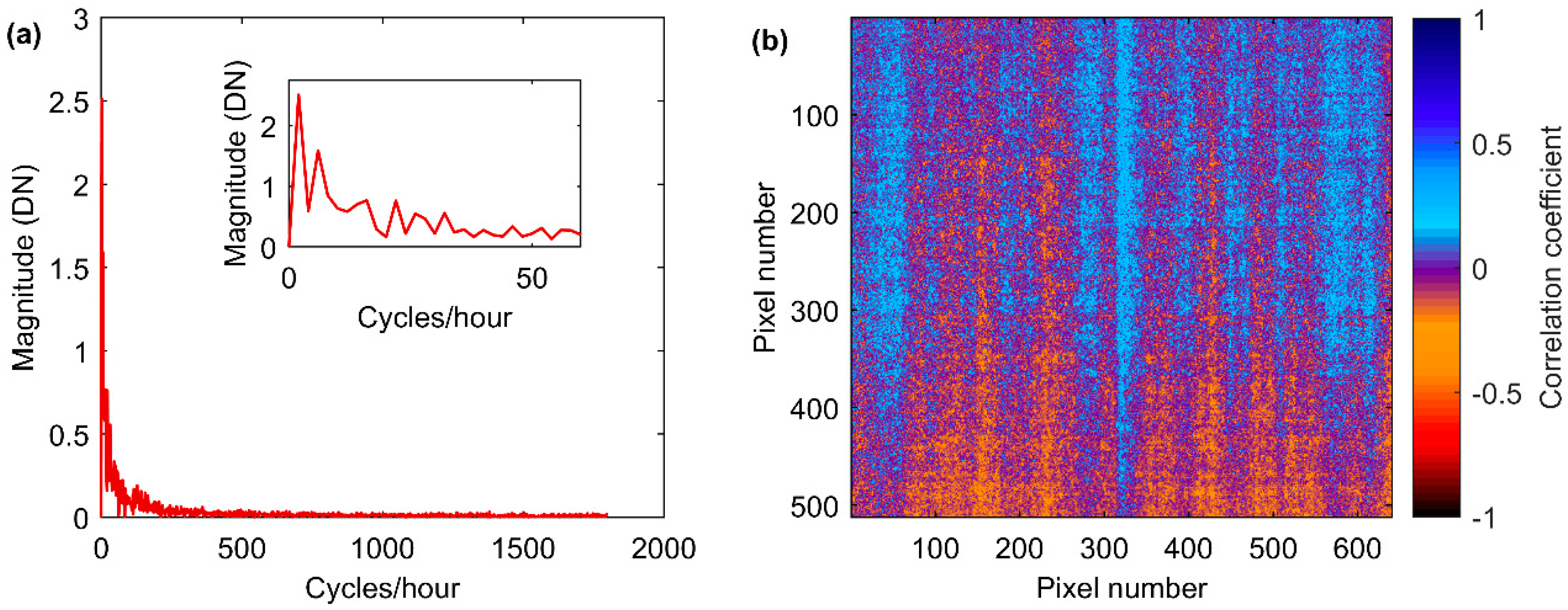
3.1.4. Sensor Noise
3.2. Field Calibration and Validation
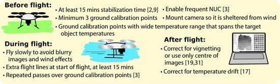
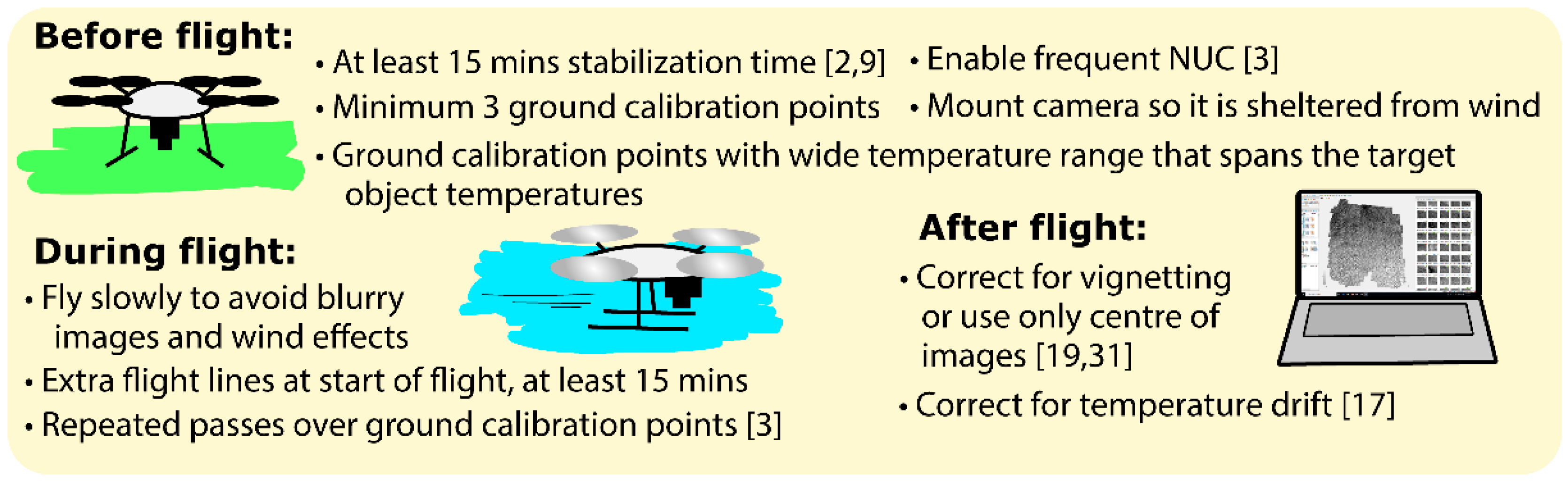
4. Discussion and Recommendations
4.1. Stabilization Time
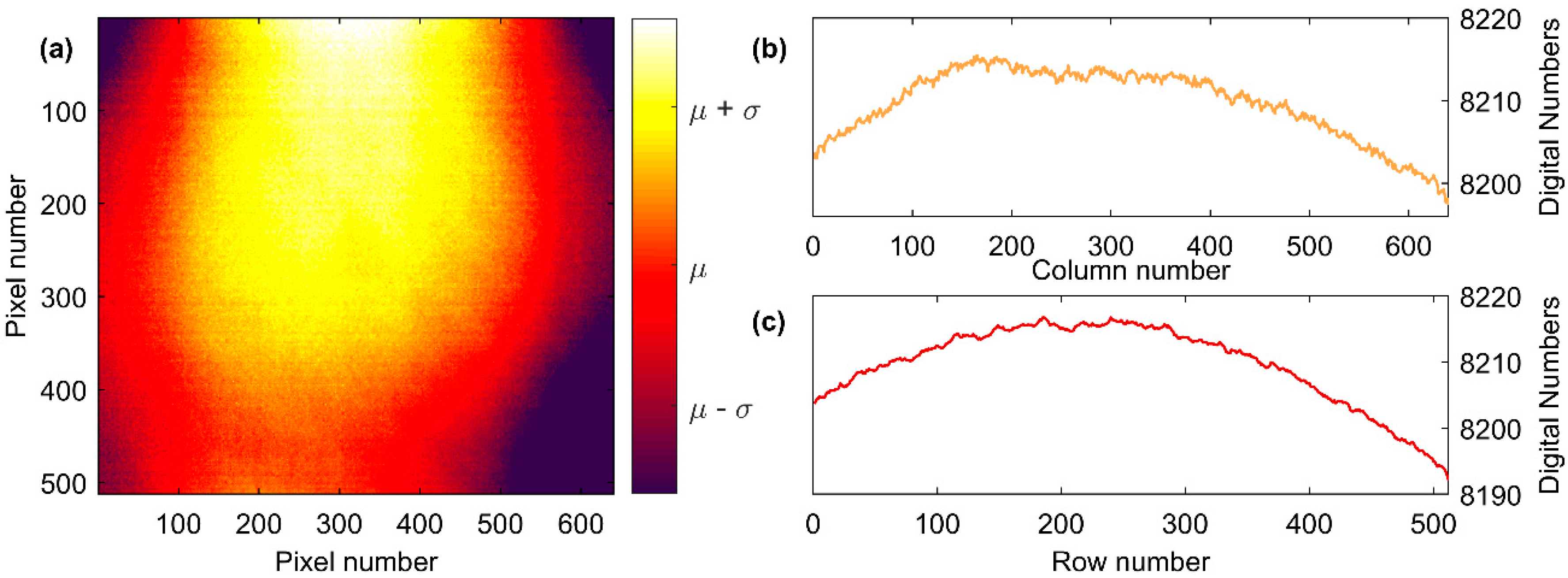
4.2. Camera Accuracy and Vignetting
4.3. Relationship between DN and Surface Temperature
4.4. Wind Effects and Temperature Drift
4.5. Field Validation
4.6. Challenges and Applicability
4.7. Future Work
5. Conclusions
Author Contributions
Funding
Acknowledgments
Conflicts of Interest
Appendix A


References
- USGS. Landsat 8 Data Users Handbook; USGS: Sioux Falls, SD, USA, 2018.
- Berni, J.A.J.; Zarco-Tejada, P.J.; Suarez, L.; Fereres, E. Thermal and Narrowband Multispectral Remote Sensing for Vegetation Monitoring From an Unmanned Aerial Vehicle. IEEE Trans. Geosci. Remote Sens. 2009, 47, 722–738. [Google Scholar] [CrossRef] [Green Version]
- Gómez-Candón, D.; Virlet, N.; Labbé, S.; Jolivot, A.; Regnard, J.L. Field phenotyping of water stress at tree scale by UAV-sensed imagery: New insights for thermal acquisition and calibration. Precis. Agric. 2016, 17, 786–800. [Google Scholar] [CrossRef]
- Gonzalez-Dugo, V.; Zarco-Tejada, P.; Berni, J.A.J.; Suárez, L.; Goldhamer, D.; Fereres, E. Almond tree canopy temperature reveals intra-crown variability that is water stress-dependent. Agric. For. Meteorol. 2012, 154–155, 156–165. [Google Scholar] [CrossRef]
- Hoffmann, H.; Jensen, R.; Thomsen, A.; Nieto, H.; Rasmussen, J.; Friborg, T. Crop water stress maps for an entire growing season from visible and thermal UAV imagery. Biogeosciences 2016, 13, 6545–6563. [Google Scholar] [CrossRef] [Green Version]
- Brenner, C.; Thiem, C.E.; Wizemann, H.D.; Bernhardt, M.; Schulz, K. Estimating spatially distributed turbulent heat fluxes from high-resolution thermal imagery acquired with a UAV system. Int. J. Remote Sens. 2017, 38, 3003–3026. [Google Scholar] [CrossRef] [PubMed] [Green Version]
- Berni, J.A.J.; Zarco-Tejada, P.J.; Sepulcre-Cantó, G.; Fereres, E.; Villalobos, F. Mapping canopy conductance and CWSI in olive orchards using high resolution thermal remote sensing imagery. Remote Sens. Environ. 2009, 113, 2380–2388. [Google Scholar] [CrossRef]
- Hoffmann, H.; Nieto, H.; Jensen, R.; Guzinski, R.; Zarco-Tejada, P.; Friborg, T. Estimating evaporation with thermal UAV data and two-source energy balance models. Hydrol. Earth Syst. Sci. 2016, 20, 697–713. [Google Scholar] [CrossRef] [Green Version]
- Smigaj, M.; Gaulton, R.; Suarez, J.C.; Barr, S.L. Use of miniature thermal cameras for detection of physiological stress in conifers. Remote Sens. 2017, 9, 957. [Google Scholar] [CrossRef]
- Sugiura, R.; Noguchi, N.; Ishii, K. Correction of low-altitude thermal images applied to estimating soil water status. Biosyst. Eng. 2007, 96, 301–313. [Google Scholar] [CrossRef]
- Jensen, A.M.; Neilson, B.T.; McKee, M.; Chen, Y. Thermal remote sensing with an autonomous unmanned aerial remote sensing platform for surface stream temperatures. In Proceedings of the 2012 IEEE International Geoscience and Remote Sensing Symposium, Munich, Germany, 22–27 July 2012. [Google Scholar]
- Stark, B.; Smith, B.; Chen, Y. Survey of thermal infrared remote sensing for Unmanned Aerial Systems. In Proceedings of the 2014 International Conference on Unmanned Aircraft Systems (ICUAS), Orlando, FL, USA, 27–30 May 2014. [Google Scholar]
- Olbrycht, R.; Więcek, B.; De Mey, G. Thermal drift compensation method for microbolometer thermal cameras. Appl. Opt. 2012, 51, 1788–1794. [Google Scholar] [CrossRef]
- Budzier, H.; Gerlach, G. Calibration of uncooled thermal infrared cameras. J. Sensors Sens. Syst. 2015, 4, 187–197. [Google Scholar] [CrossRef] [Green Version]
- Nugent, P.W.; Shaw, J.A.; Pust, N.J. Correcting for focal-plane-array temperature dependence in microbolometer infrared cameras lacking thermal stabilization. Opt. Eng. 2013, 52, 061304. [Google Scholar] [CrossRef] [Green Version]
- Ribeiro-Gomes, K.; Hernández-López, D.; Ortega, J.F.; Ballesteros, R.; Poblete, T.; Moreno, M.A. Uncooled thermal camera calibration and optimization of the photogrammetry process for UAV applications in agriculture. Sensors 2017, 17, 2173. [Google Scholar] [CrossRef] [PubMed]
- Mesas-Carrascosa, F.J.; Pérez-Porras, F.; de Larriva, J.E.M.; Frau, C.M.; Agüera-Vega, F.; Carvajal-Ramírez, F.; Martínez-Carricondo, P.; García-Ferrer, A. Drift correction of lightweight microbolometer thermal sensors on-board unmanned aerial vehicles. Remote Sens. 2018, 10, 615. [Google Scholar] [CrossRef]
- Smigaj, M.; Gaulton, R.; Barr, S.L.; Suarez, J.C. Investigating the performance of a low-cost thermal imager for forestry applications. In Proceedings of the Image and Signal Processing for Remote Sensing XXII, Edinburgh, UK, 26–28 September 2016. [Google Scholar]
- Meier, F.; Scherer, D.; Richters, J.; Christen, A. Atmospheric correction of thermal-infrared imagery of the 3-D urban environment acquired in oblique viewing geometry. Atmos. Meas. Tech. 2011, 4, 909–922. [Google Scholar] [CrossRef] [Green Version]
- Aubrecht, D.M.; Helliker, B.R.; Goulden, M.L.; Roberts, D.A.; Still, C.J.; Richardson, A.D. Continuous, long-term, high-frequency thermal imaging of vegetation: Uncertainties and recommended best practices. Agric. For. Meteorol. 2016, 228, 315–326. [Google Scholar] [CrossRef] [Green Version]
- Hammerle, A.; Meier, F.; Heinl, M.; Egger, A.; Leitinger, G. Implications of atmospheric conditions for analysis of surface temperature variability derived from landscape-scale thermography. Int. J. Biometeorol. 2017, 61, 575–588. [Google Scholar] [CrossRef]
- Olbrycht, R.; Więcek, B. New approach to thermal drift correction in microbolometer thermal cameras. Quant. Infrared Thermogr. J. 2015, 12, 184–195. [Google Scholar] [CrossRef]
- FLIR Tech Note: Radiometric Temperature Measurements. Available online: https://www.flir.com/globalassets/guidebooks/suas-radiometric-tech-note-en.pdf (accessed on 20 November 2018).
- Palmer, J.M. The measurement of transmission, absorption, emission, and reflection. In Handbook of Optics—Volume II: Devices, Measurements and Properties; Bass, M., Van Stryland, E.W., Williams, D.R., Wolfe, W.L., Eds.; McGraw-Hill, Inc.: New York, NY, USA, 1995; pp. 25.1–25.25. ISBN 0-07-047974-7. [Google Scholar]
- Mölder, M.; Kellner, E. Excess resistance of bog surfaces in central Sweden. Agric. For. Meteorol. 2002, 112, 23–30. [Google Scholar] [CrossRef]
- Kettridge, N.; Baird, A. Modelling soil temperatures in northern peatlands. Eur. J. Soil Sci. 2008, 59, 327–338. [Google Scholar] [CrossRef]
- Royer, A.; Bussieres, N.; Goita, K. Characterization of land surface thermal structure from NOAA-AVHRR data over a northern ecosystem. Remote Sens. Environ. 1997, 60, 282–298. [Google Scholar]
- Maes, W.H.; Huete, A.R.; Steppe, K. Optimizing the processing of UAV-based thermal imagery. Remote Sens. 2017, 9, 476. [Google Scholar] [CrossRef]
- Mitchell, H.B. Image Fusion: Theories, Techniques and Applications; Springer-Verlag: Berlin/Heidelberg, Germany, 2010; Volume 134, ISBN 9783642112157. [Google Scholar]
- Goldman, D.B. Vignette and Exposure Calibration and Compensation. IEEE Trans. Pattern Anal. Mach. Intell. 2010, 32, 2276–2288. [Google Scholar] [CrossRef] [PubMed]
- Aasen, H.; Honkavaara, E.; Lucieer, A.; Zarco-Tejada, P.J. Quantitative remote sensing at ultra-high resolution with UAV spectroscopy: A review of sensor technology, measurement procedures, and data correction work flows. Remote Sens. 2018, 10, 1091. [Google Scholar] [CrossRef]
- Pix4D SA. Pix4Dmapper 4.1 User Manual. Available online: https://support.pix4d.com/hc/en-us/articles/204272989-Offline-Getting-Started-and-Manual-pdf- (accessed on 20 November 2018).
- Zhou, H.X.; Lai, R.; Liu, S.Q.; Jiang, G. New improved nonuniformity correction for infrared focal plane arrays. Opt. Commun. 2005, 245, 49–53. [Google Scholar] [CrossRef]
- Jensen, A.M.; Mckee, M. Calibrating thermal imagery from an unmanned aerial vehicle AggieAir. In Proceedings of the 2013 IEEE International Geoscience and Remote Sensing Symposium, Melbourne, VIC, Australia, 21–26 July 2013. [Google Scholar]
- Turner, D.; Lucieer, A.; Malenovský, Z.; King, D.H.; Robinson, S.A. Spatial co-registration of ultra-high resolution visible, multispectral and thermal images acquired with a micro-UAV over antarctic moss beds. Remote Sens. 2014, 6, 4003–4024. [Google Scholar] [CrossRef]
- Horny, N. FPA camera standardisation. Infrared Phys. Technol. 2003, 44, 109–119. [Google Scholar] [CrossRef]
- Kaltenbach, H.-M. A Concise Guide to Statistics; Springer: Berlin/Heidelberg, Germany, 2012; ISBN 9783642235023. [Google Scholar]
- Smigaj, M.; Gaulton, R.; Barr, S.L.; Suárez, J.C. UAV-Borne thermal imaging for forest health monitoring: Detection Of disease-induced canopy temperature increase. Int. Arch. Photogramm. Remote Sens. Spat. Inf. Sci. 2015, 40, 349–354. [Google Scholar] [CrossRef]
- Kim, Y.; Still, C.J.; Hanson, C.V.; Kwon, H.; Greer, B.T.; Law, B.E. Canopy skin temperature variations in relation to climate, soil temperature, and carbon flux at a ponderosa pine forest in central Oregon. Agric. For. Meteorol. 2016, 226–227, 161–173. [Google Scholar] [CrossRef]
- Goodall, T.R.; Bovik, A.C.; Paulter, N.G. Tasking on natural statistics of infrared images. IEEE Trans. Image Process. 2016, 25, 65–79. [Google Scholar] [CrossRef]
- Aasen, H.; Bolten, A. Multi-temporal high-resolution imaging spectroscopy with hyperspectral 2D imagers—From theory to application. Remote Sens. Environ. 2018, 205, 374–389. [Google Scholar] [CrossRef]
- Burkart, A.; Aasen, H.; Alonso, L.; Menz, G.; Bareth, G.; Rascher, U. Angular dependency of hyperspectral measurements over wheat characterized by a novel UAV based goniometer. Remote Sens. 2015, 7, 725–746. [Google Scholar] [CrossRef]
- Duffour, C.; Lagouarde, J.P.; Roujean, J.L. A two parameter model to simulate thermal infrared directional effects for remote sensing applications. Remote Sens. Environ. 2016, 186, 250–261. [Google Scholar] [CrossRef]


| Name | Date | Start Time | Stabilization Time (min) | Flight Time (min) | Number of Images | Number of TCPs | Flight Altitude (m) | Resolution (cm/pixel) | Analysis |
|---|---|---|---|---|---|---|---|---|---|
| A | 28 June 2017 | 10:44 | 15 | 11 | 448 | 4 | 50 | 6.3 | Sensitivity |
| B | 11 July 2018 | 19:52 | 20 | 8 | 108 | 4 | 61 | 7.5 | Sensitivity |
| C | 12 July 2018 | 14:47 | 0 1 | 4 | 39 | 3 | 53 | 6.8 | Validation |
| D | 12 July 2018 | 20:27 | 15 | 2 | 58 | 3 | 53 | 6.8 | Validation |
| Flight | Calibration | R2-adj | p-Value | Mean image DN | R2-adj | p-Value |
|---|---|---|---|---|---|---|
| A | DN = 20.8(TCP) + 7601 | 0.99 | <0.01 | DN = 12.4(mins) + 8157 | 0.46 | <0.001 |
| B | DN = 20.6(TCP) + 8950 | 0.97 | <0.01 | DN = 14.6(mins) + 9411 | 0.74 | <0.001 |
| C | DN = 22.7(TCP) + 8861 | 0.99 | <0.01 | DN = 43.0(mins) + 9670 | 0.34 | <0.001 |
| D | DN = 15.2(TCP) + 9050 | 0.99 | <0.05 | DN = 0.37(mins) + 9416 | 0 | >0.05 |
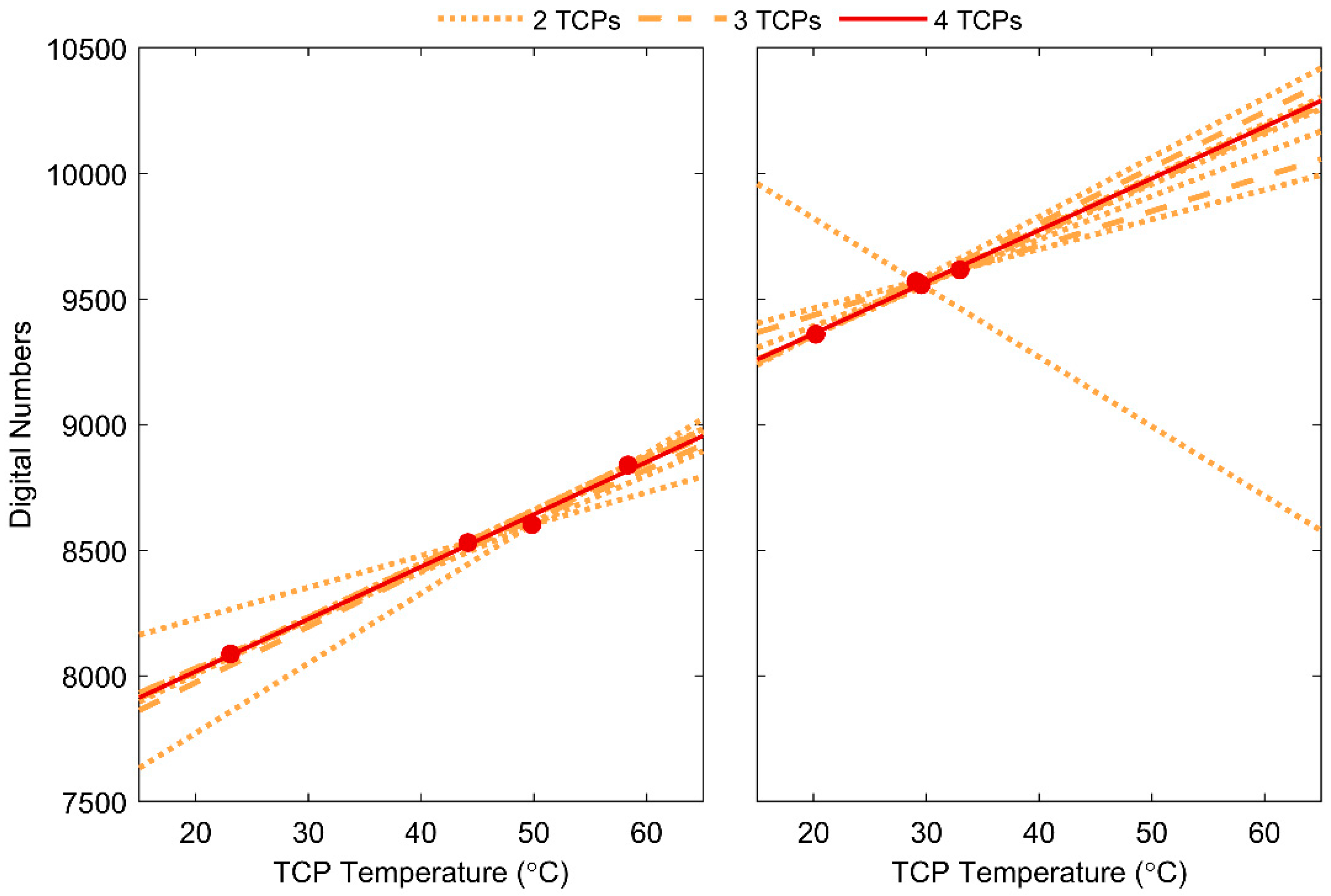
| Flight | 4 TCP Mean (°C) | Max Δ 3 (°C) | Min Δ 3 (°C) | Max Δ 2 (°C) | Min Δ 2 (°C) |
|---|---|---|---|---|---|
| A | 29.5 | 1.4 | 0.15 | 10.3 | 0.17 |
| B | 25.1 | 2.8 | 0.02 | 7.7 | 0.17 |
© 2019 by the authors. Licensee MDPI, Basel, Switzerland. This article is an open access article distributed under the terms and conditions of the Creative Commons Attribution (CC BY) license (http://creativecommons.org/licenses/by/4.0/).
Share and Cite
Kelly, J.; Kljun, N.; Olsson, P.-O.; Mihai, L.; Liljeblad, B.; Weslien, P.; Klemedtsson, L.; Eklundh, L. Challenges and Best Practices for Deriving Temperature Data from an Uncalibrated UAV Thermal Infrared Camera. Remote Sens. 2019, 11, 567. https://0-doi-org.brum.beds.ac.uk/10.3390/rs11050567
Kelly J, Kljun N, Olsson P-O, Mihai L, Liljeblad B, Weslien P, Klemedtsson L, Eklundh L. Challenges and Best Practices for Deriving Temperature Data from an Uncalibrated UAV Thermal Infrared Camera. Remote Sensing. 2019; 11(5):567. https://0-doi-org.brum.beds.ac.uk/10.3390/rs11050567
Chicago/Turabian StyleKelly, Julia, Natascha Kljun, Per-Ola Olsson, Laura Mihai, Bengt Liljeblad, Per Weslien, Leif Klemedtsson, and Lars Eklundh. 2019. "Challenges and Best Practices for Deriving Temperature Data from an Uncalibrated UAV Thermal Infrared Camera" Remote Sensing 11, no. 5: 567. https://0-doi-org.brum.beds.ac.uk/10.3390/rs11050567