1. Introduction
The survey and quantification of woody debris left over from harvesting operations on managed forests is an important part of forestry operations. Post-harvest debris plays an important role in maintaining the quality of a site, by promoting nutrient and water retention, and providing a temperature-stabilized micro-climate for soil organisms that promote forest regrowth [
1,
2]. Post-harvest debris also has potential use as a source of biofuel [
3]; accurate quantification of debris left over from harvesting allows for appropriate quantities of debris to be extracted, while ensuring sustainable forest management is achieved. The quantification of post-harvest Coarse Woody Debris (CWD) (i.e., larger pieces of debris arising from a tree’s stem, as opposed to small branches or slash) is also an important step in reconciling differences between pre-harvest estimates of timber yield (i.e., derived from either in-field or LiDAR-based census/imputation [
4]) and actual timber yield achieved at harvest. Differences between estimated and actual yields may arise due to errors in pre-harvest inventories or sub-optimal harvesting operations (i.e., sub-optimal bucking of trees into logs [
5]) that result in variations in the amount of CWDs left over at a site after harvest. The ability to quantify CWDs at a post-harvest site therefore potentially allows for a “reconciliation” between these causes to be made, which is an important step in improving future inventories (i.e., by correcting or fine-tuning inventory models).
Measurements of post-harvest debris have traditionally been made using manual counting/sampling methods in the field such as sample plot inventory and line-transect intercept methods [
6]. Although these methods are accurate at the scale of the sample plot, and allow for a distinction to be made between coarse versus fine woody debris, they are extremely labor-intensive and do not necessarily provide good estimates of debris over large areas. Methods based on aerial photography and/or remote sensing are often less time-consuming and labor-intensive than their ground-based counterparts, and have been used to measure piles of residue [
7] or scattered debris [
8,
9,
10,
11] using imagery, LiDAR, synthetic aperture radar, spectrometer data, or some combination of them. The majority of existing remotely sensed-based approaches rely on either manual interpretation of imagery or indirect inference of woody debris quantity (i.e., volume, ground cover etc.) from properties of the image such as surface height and image texture, owing to the limited spatial resolution available from, for example, manned aircraft. Low-flying Unmanned Aerial Vehicles (UAVs), or “drones”, provide the ability to collect high-spatial-resolution imagery for quantifying debris in clear cut areas, but challenges remain in the interpretation of this imagery into measurements of debris of different size classes in an automated way.
In this paper, we propose and evaluate new automated methods for the collection and interpretation of high-resolution, UAV-borne imagery over post-harvested forests for estimating quantities of fine and CWD. Using high-resolution, color geo-registered mosaics generated from UAV-borne images, we develop manual and automated processing methods for detecting, segmenting and counting both fine and CWD, including tree stumps. Automated methods are developed based on deep learning image processing techniques such as Convolutional Neural Networks (CNNs) [
12,
13] for detecting individual stumps/logs and segmenting the surface of the woody material from background image data. Algorithms are then developed to measure key geometric parameters from each piece of woody debris/stump (i.e., length, diameter) to evaluate the total volume of woody material, while providing a distinction between classes of debris (i.e., coarse vs. fine debris). Results of these methods are compared against sample plot measurements of debris made in the field and measurements derived from manual annotation of high-resolution aerial images.
1.1. Remote Sensing and Airborne Measurements of Woody Debris
On a post-harvest site, there are typically two conditions that logging residue is left in: individual pieces dispersed across the site or piles created by machines. Estimation of volume from machine-created piles has been performed using both ground-based and remotely sensed methods. Measuring pile volume is simplified by the fact that occluding material is often separated from piles, and the dimensions of each pile can be measured directly for example by using geometric measurements, terrestrial laser scanning [
14] and/or terrestrial/aerial photogrammetry [
15] on manually segmented piles. Trofymow et al. [
7] compared the accuracy in volume estimation of machine-piled logging residue between simple ground-based geometry calculations and remote sensing methods using LiDAR/orthophotography from manned aircraft, and concluded that remote sensing methods gave superior results. Eamer and Walker [
8] developed an automated approach to segment logs using a combination of LiDAR and orthophotography to quantify the sand storage capacity of logs. In this work, the logs were scattered, rather than being in piles, and thus they required a faster approach, using supervised classification to identify the logs. Logs were easily discernible due to the homogeneous background color of the sands and no distinction was made between coarse and fine woody debris.
Regarding detecting and mapping woody debris in scattered and unstructured environments, several approaches have been developed. Smikrud and Prakash [
11] developed an approach to detecting scattered large woody debris in aerial photographs in riverine environments. An automatic image processing pipeline was developed consisting of high-pass filtering of the second principal image component, low-pass filtering, and thresholding to differentiate between wood and no-wood areas. This method of classification does not distinguish between different sizes of woody debris. Similarly, Ortega et al. [
10] used a photogrammetry approach with orthophotos captured from a digital camera mounted on a tandem minitrike (a form of low-cost aircraft) to map the aerial coverage of large woody debris and snags in rivers. Neither of these approaches were able to estimate the actual volume of woody material nor distinguish between different size classes of debris. Regarding remote sensing methods that indirectly measure woody debris, Huang et al. [
9] developed an approach to mapping CWD areal coverage in a post-fire forest using low spatial resolution airborne Synthetic Aperture Radar (SAR) and Airborne Visible/Infrared Imaging Spectrometer (AVIRIS) sensors by regressing a relationship between CWD quantity and sensed backscatter parameters. They achieved a relatively low correlation coefficient of 0.54 between CWD areal coverage and sensor parameters.
UAVs or ‘drones’, a low-cost alternative to manned aircraft, have also been explored as a potential method of estimating the volume of post-harvest CWD residue. UAVs have the potential to operate at lower altitudes than manned fixed-wing aircraft or helicopters (hence producing higher resolution imagery), but have a lower payload carrying capacity, and hence are typically restricted to carrying imaging sensors in practical operations (as opposed to LiDAR, which typically requires the use of a larger, (manned) aircraft). Davis [
16] used UAV-borne imagery and structure from motion/photogrammetry to create 2 cm per-pixel imagery and digital surface models of a post-harvest forest and automatically estimate the volume of both scattered and machine-piled log residue. The DSM was computed before log pixels were separated from the background using a mean-shift segmentation and thresholding of the red channel of the orthomosaic. Once a CWD mask was obtained, the DSM of the estimated background and logs were subtracted from one another and multiplied by the cell resolution. The results were varied, with the UAV predicted volume error for individual 10 m × 10 m plots ranging from 1% to 842% (over-estimation) when compared with ground measurements. Challenges remained in the algorithm adapting to varying backgrounds, with poor performance observed when the background had high reflectance in the red channel of the imagery. Regarding works focused on tree stumps, Puliti et al. [
17] used an iterative region-growing approach to detect tree stumps in photogrammetry collected from a UAV. Results showed that tree stumps could be detected with an accuracy of 68–80%. Samiappan et al. [
18] used traditional computer vision techniques such as Hough transform with drone imagery to count tree stumps with an accuracy of 77% and estimate their diameter with an RMSE of 4.3 cm.
1.2. Advances in Computer Vision and Deep Learning
In recent years there have been several breakthroughs in image recognition within the field of computer vision. CNNs, a deep learning approach developed decades ago for automatic recognition of zip code data [
12], have had a resurgence of interest with the advent of increasingly powerful computers and the availability of large datasets. CNNs have been used to achieve record breaking performance on many benchmark datasets, using large parameterized models with multiple layers of feature learners. CNNs learn generic low-level features such as edges in their early layers and higher-level features such as shapes which are more class specific in their upper layers [
12,
13]. The adoption of CNNs in computer vision have signaled a shift in the literature from analytical, model-based approaches where features are engineered towards data-driven approaches where features are learnt.
The field of remote sensing has progressively adopted CNN approaches for tasks involving image recognition [
19]. While object detection from high altitudes remains a more difficult task than traditional object detection from ground-based platforms, CNNs have been used to detect objects such as aircraft, ships, oil tanks, basketball courts and tennis courts from aerial and satellite images [
20,
21,
22,
23,
24,
25]. Pixelwise labelling of images captured from airborne and spaceborne platforms has been approached using CNN architectures designed for semantic segmentation in the computer vision literature.
1.3. Contributions of Our Approach
Past approaches to measuring woody debris in post-harvest forests using remotely sensed data have had limited success in working in environments where debris is scattered, or at distinguishing between different size classes of debris (i.e., fine versus coarse debris), which is a necessary step in estimating the total volume of debris when debris is scattered. In this paper, we exploit recent developments in computer vision and deep learning to perform accurate detection and segmentation of individual pieces of woody debris in an automatic way, using high-spatial-resolution imagery available from a UAV, hence allowing for the quantification of woody debris volume over unstructured sites. The use of image interpretation (as opposed to relying on additional sensors such as LiDAR) facilitates the use of lightweight UAVs for survey and data collection, providing a cost-effective assessment methodology.
2. Materials and Methods
2.1. Study Area and Imagery Surveys
In October 2015, fieldwork was undertaken at the Canobolas State Forest (33
22
S 149
02
E), New South Wales, Australia over a harvested compartment of pine trees (
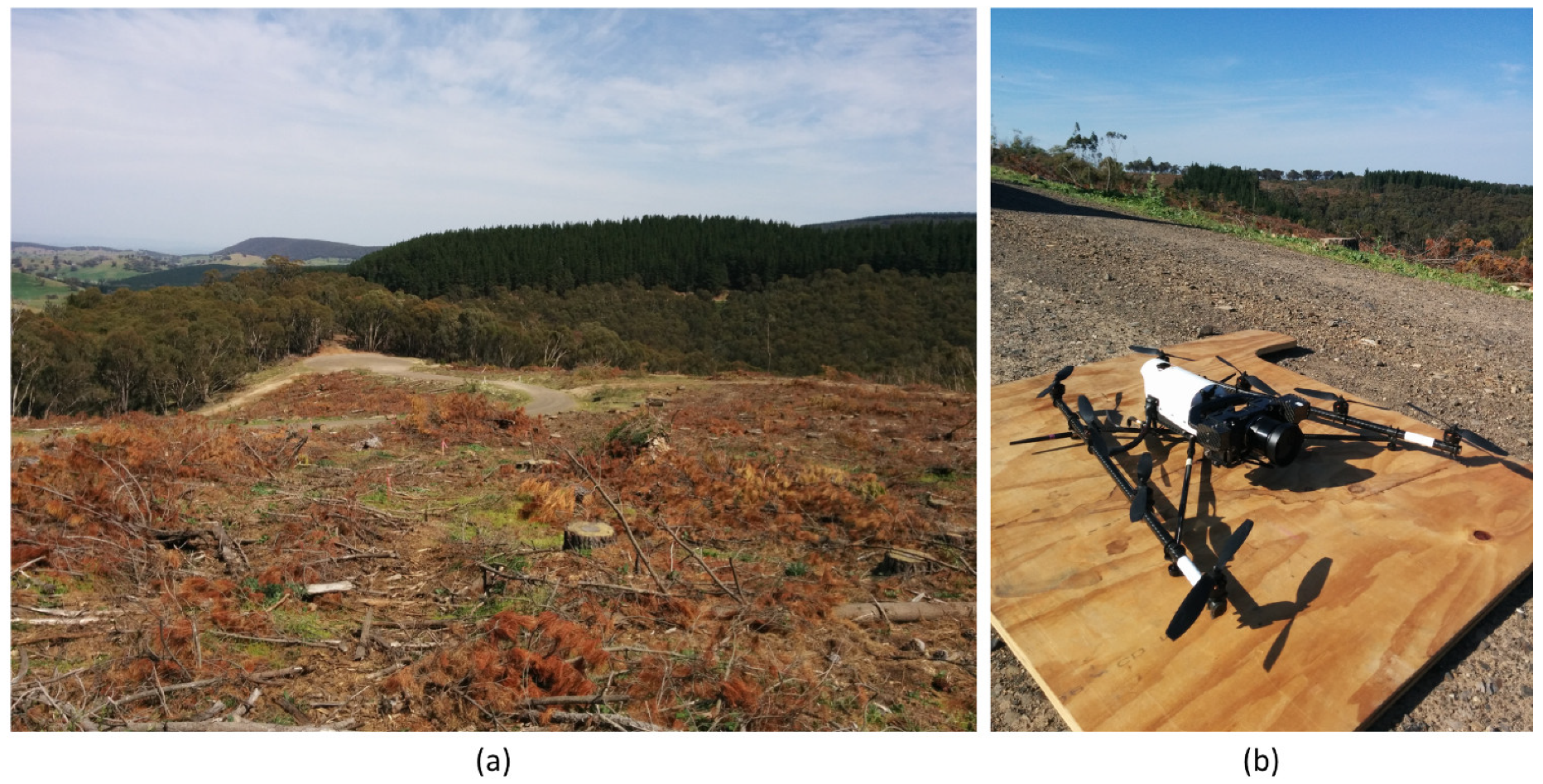
Pinus radiata). Harvesting at the site had occurred in May 2015, and the site was characterized by a combination of coarse and fine woody debris, partially senesced and live pine needles, bare ground, weeds, and shrubs (see
Figure 1a).
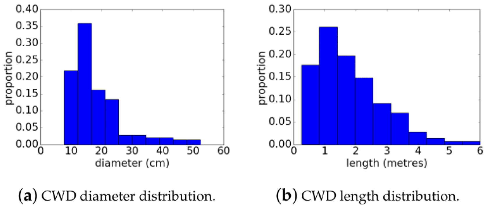
At the study site, nine sampling quadrats were selected, each a 10-by-10 m square region of ground. Plots were characterized visually to have either a ‘low’, ‘medium’ or ‘high’ quantity of debris and plot locations were selected to achieve three plots for each of these classifications. Plot locations were measured by tape measure and marked out using survey poles. Survey-grade (cm-accuracy) Differential-GPS (DGPS) was used to measure the locations of the plot corner coordinates, and these were marked using 15-by-15 cm purple visual targets to ensure plot boundaries were visible from the air during UAV survey. Subsequent to the UAV flights, in situ measurements of woody debris were made by hand in the field. Survey-grade DGPS was used to measure the location of each and every stump located in each plot, with diameters and heights of each stump measured by hand using a tape measure. Within each plot, all pieces of wood with diameter greater than 2.5 cm were manually measured in the field using calipers and a tape measure. The length and diameter of all pieces was recorded, and wood marked with spray paint to avoid double-counting.
An AscTec Falcon-8 UAV, (
Figure 1b) was flown over the study site to collect geo-referenced color imagery. The UAV uses eight controlled rotors and an on-board navigation system using inertial sensors and GPS to provide fully autonomous trajectory following control over a pre-arranged flight path. Takeoff and landing of the UAV was performed manually by an experienced remote aircraft pilot from a 1-by-1 m wooden board (placed on an adjacent road) with a laptop-based ground station operated from the back of a parked four-wheel drive. The AscTec Falcon-8 can fly at altitudes from 10–100 m with an endurance of approximately 15 min. The UAV carried a consumer-grade color digital camera with a resolution of 24 MPix, which provided a resolution on the ground of approximately 2 mm per pixel at 15 m altitude and 4 mm per pixel at 30 m altitude. A single flight at 30 m altitude was used to cover the entire study site of approximately 4.5 hectares and four targeted flights at 10–15 m altitudes (variations due to changes in topographic elevation) were used to cover all of the 10-by-10 m sample plot areas at the highest possible resolution (approximately 2 mm per pixel). All UAV flights were performed in the morning of the 7 October 2015.
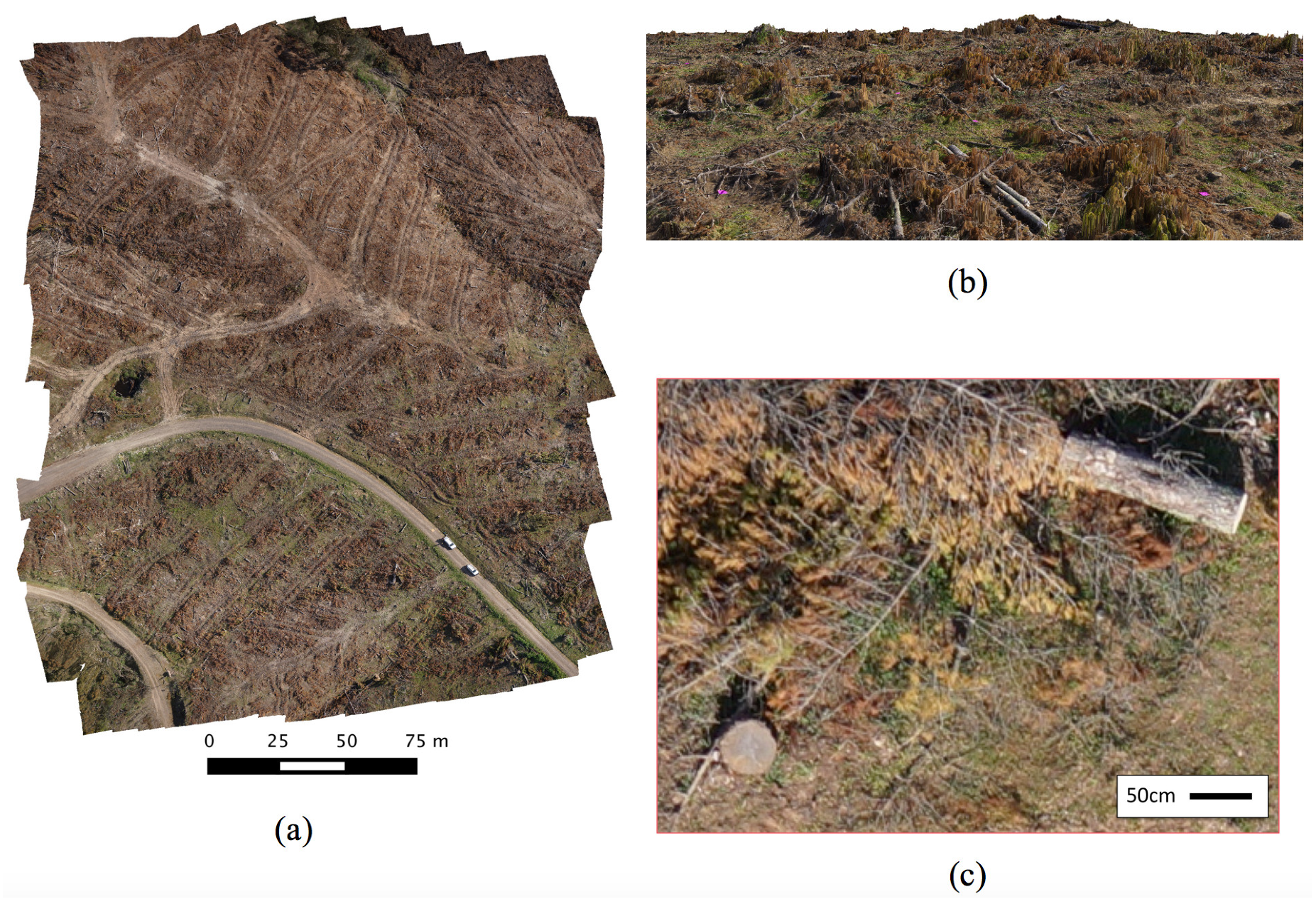
Collected images were post-processed using a structure-from-motion/ photogrammetry software package Agisoft Photoscan (
http://www.agisoft.com/) (also using on-board UAV navigation data) to produce high-resolution geo-referenced imagery mosaics and digital surface models (
Figure 2). All parameters in the software were set to “high-accuracy” and “high-resolution” and the digital surface model was constructed using the “height field” option.
2.2. Manual Analysis of High-Resolution Imagery
For each of the imagery mosaics over the 10 × 10 m plots, stumps and all visible woody material with a diameter greater than 2.5 cm were manually annotated using ImageJ version 1.41 (
https://imagej.nih.gov/ij/) and visualized using QGIS version 2.8 (
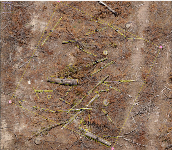
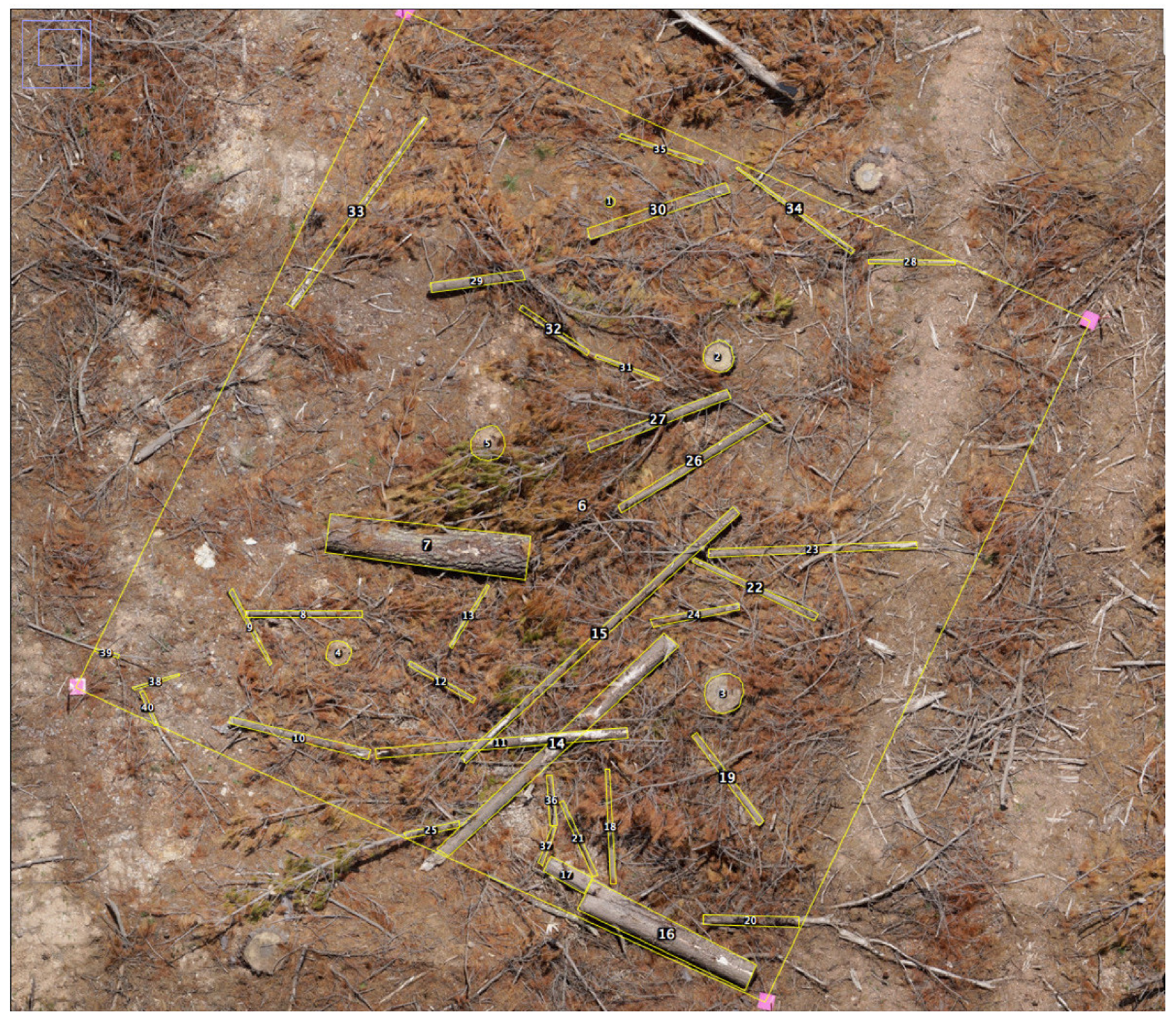
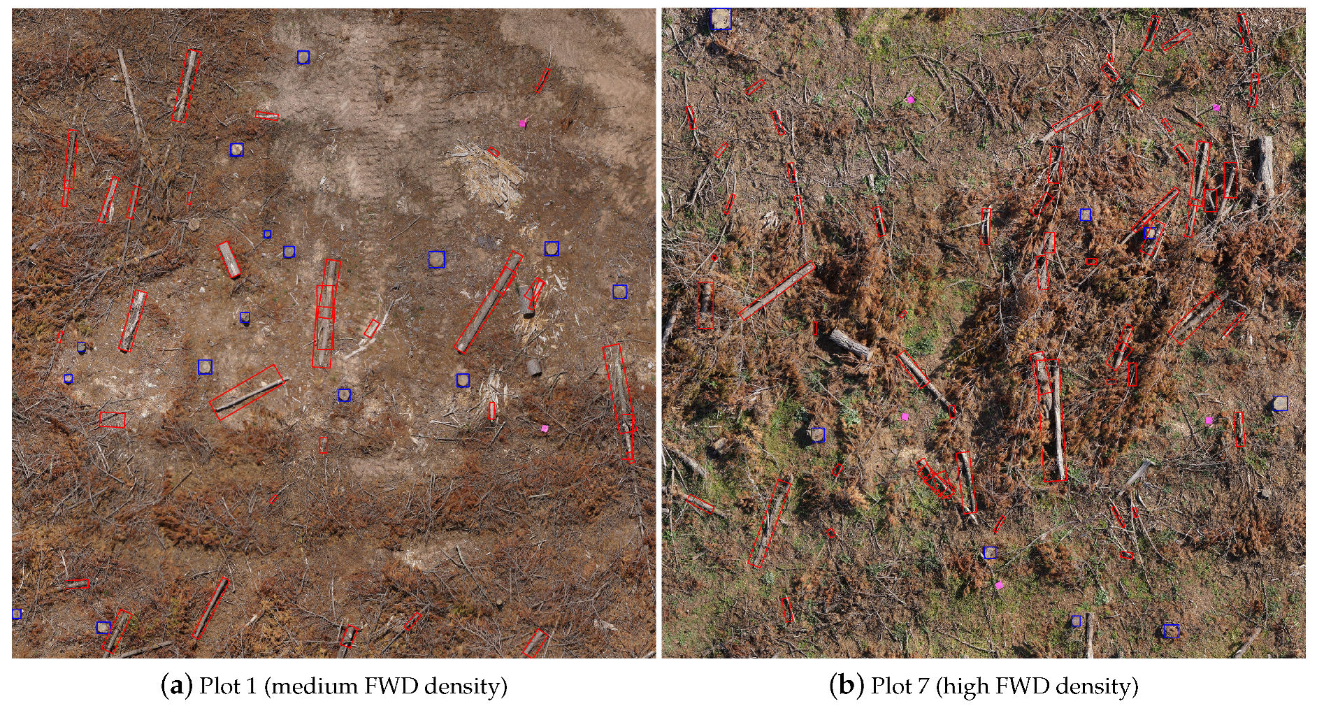
http://www.qgis.org). CWD was defined in this study as larger pieces of debris, with a diameter >10 cm, arising from a tree’s stem or large branch, as opposed to the smaller branches (Fine Woody Debris (FWD)), foliage or bark. The coordinates of all visible CWD and the outlines of stumps were annotated by manually clicking on the imagery coordinates corresponding to the outline of each piece of visible wood or stump, hence creating a separate closed polygon in the two-dimensional coordinates of the image for each piece (
Figure 3). All polygon coordinates were transformed from image coordinates into horizontal Northing and Easting coordinates in meters using the geo-registration parameters of the imagery mosaic.
For each polygon corresponding to a piece of woody debris (coarse and fine debris, excluding stumps), scripts were used to compute the major and minor axes of the polygon in the horizontal X-Y plane. Polygons were then approximated as cylinders with length provided as the major axis of the annotated polygon and diameter from the minor axis of the polygon. The volume (V) of each piece was then calculated using Equation (
1):
where
l is the length and
d is the diameter. To clarify,
d here represents the average diameter. The same calculation for volume was applied to the list of in situ, manually measured wood from the field (diameters and lengths) to yield reference measurements of total log timber volume for each plot.
For visible stumps, the outlines recorded in the annotated polygons were used to calculate the average diameter and cross-sectional area at the height for which the tree had been felled. In order to estimate the volume of each tree stump from the annotated polygon, information about the stump height was extracted from the digital surface height model imagery layer provided through structure-from-motion image processing. For each annotated stump (circular polygon drawn around stump boundary), another polygon was automatically created, a doughnut shape, extending out 10 cm from the stump boundary. The height of the stump was calculated by taking the mean elevation of all pixels from the digital surface model imagery layer inside the original stump polygon and subtracting the minimum elevation measurement from within the second doughnut shaped polygon (approximating a region of ground around the stump). This height was then multiplied by the cross-sectional area of each stump to approximate the stump volume.
2.3. Automated Stump Detection
The Faster-RCNN [
26] object detector was used to detect tree stumps in the plot images. The detector uses a CNN to extract feature maps from the image. Bounding boxes are proposed from the feature maps using a Region Proposal Network (RPN). These bounding boxes are then fed back into a CNN for classification of their content and refinement of the box coordinates. The parameters of Faster-RCNN are learnt by training the network with images of objects that have been annotated with a bounding box and classification label. The network parameters are incrementally optimized to reduce a cost that is a function of the error of the predicted bounding box coordinates and class label.
The Faster-RCNN stump detector was pre-trained on the MS COCO dataset [
27], before being fine-tuned on the annotated stump data. The MS COCO dataset was curated for computer vision research and contains a variety of generic object classes. It is common practice to use a dataset such as MS COCO to pre-train networks, as many of the low-level image features, such as edges and lines, generalize to any object class. The parameters used for training the stump detector, selected based on those used in [
26], are summarized in
Table 1. The annotated stump data consisted of positive and negative examples of stumps. Negative examples were split into three separate classes, including logs, the pink markers used to identify boundaries in the field and a background class which contained images of things that looked similar to stumps (for example, patches of dirt that had a circular shape or small sections of gravel). This was to reduce the number of false positive detections.
The plot mosaics were large (each side was roughly between 5800–8800 pixels). Due to the computational constraints of the Faster-RCNN network on the image size, once trained, the detector was made to perform inference on a pixel sliding window. The coordinates of bounding boxes corresponding to detections of stumps made in these windows were then converted to the global plot coordinates. The sliding window was made to convolve over the image with a stride of 400 pixels in both the horizontal and vertical directions, thus having an overlap of 200 pixels. This is because of the high likelihood that all stumps are smaller than 200 pixels (i.e., 67.80 cm). The overlap was used to guarantee a full view of every stump in at least one of the detection windows. This is important as the detector was trained on full stumps rather than partial stumps. If there is no a priori knowledge of the stump size, then a larger overlap can be used at the expense of computation time.
The overlapping sliding window introduced duplicate bounding boxes pertaining to partial and full views of the same stumps from several different windows. Redundant boxes were eliminated by leveraging the known shape of the stumps (a circle). Stumps detected from a full view are most likely to be square, while those detected from a partial view are more likely to be rectangular. To suppress all but the boxes associated with full views, boxes with close proximity i.e., their centers within 150 pixels of each other, were grouped together and all boxes other than the squarest one (all sides closest to being equal) were removed.
2.4. Automated CWD Volume Estimation
The pipeline for automatically estimating the volume of CWD from aerial imagery is divided into three main steps: log detection, segmentation, and rectangle fitting. Scattered CWD in a plot are detected and segmented at the pixel level, with rectangles then fitted to each log. By approximating the logs as cylinders (which have a diameter that is constant in the image and depth axes), the rectangle dimensions can be used to estimate the volume of each without the need for any DSM or other 3D information.
Section 2.4.1 gives an overview of the whole method and
Section 2.4.2,
Section 2.4.3 and
Section 2.4.4 describe the log detection, segmentation, and rectangle fitting and refinement components in more detail.
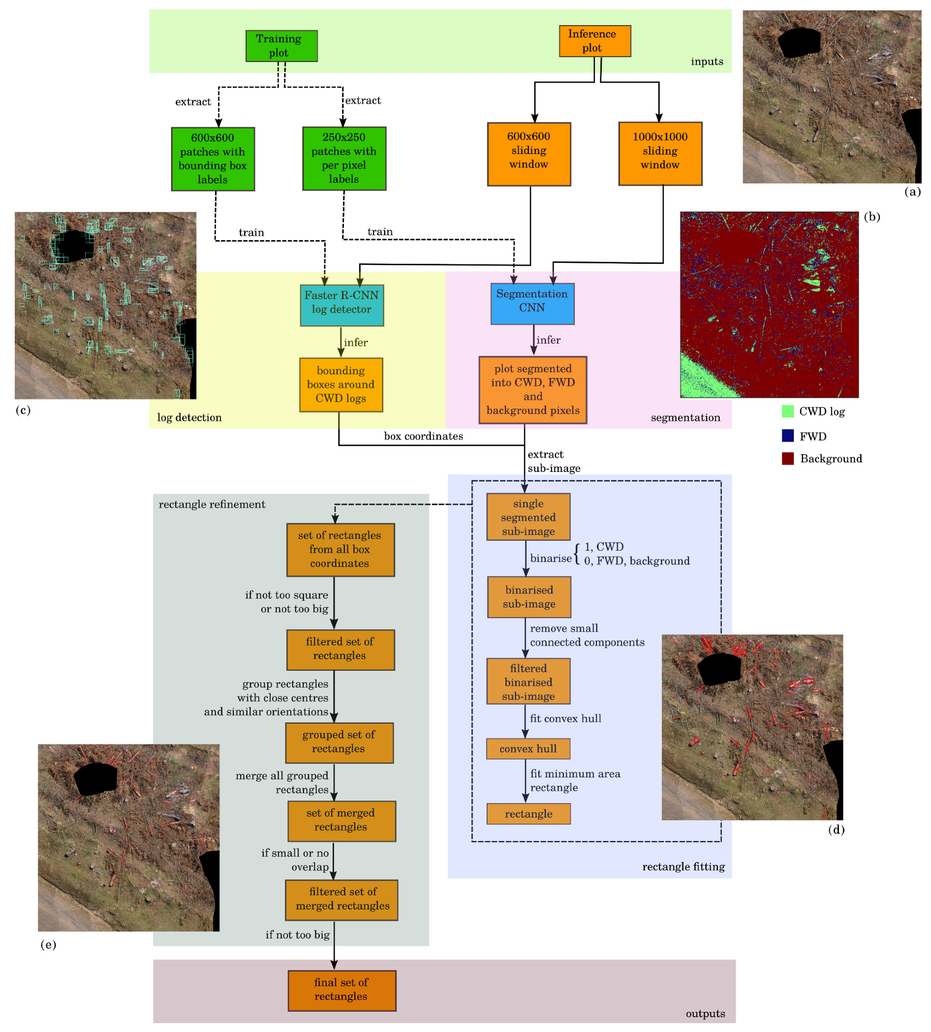
2.4.1. Summary of Algorithm
The overall process is comprised of a training and inference phase. In the training phase, a Faster-RCNN CWD detector and segmentation network are individually trained on images extracted from a given plot mosaic allocated for training. Once the models are trained, new plot mosaics are passed through the pipeline for detection, segmentation, and rectangle fitting to estimate the volume of CWD in the scene (the inference phase). The log detection module provides axis aligned bounding boxes containing CWD and the segmentation module provides per-pixel identification of CWD. The pixel identification has a finer spatial scale, but there are significant false positives as there is less object knowledge used. The log detection uses object knowledge and hence has less false positives, but the result is coarse. The rectangle fitting module fuses these two pieces of information together. Using techniques from computational geometry, rectangular bounding boxes are fitted that are aligned with the major and minor axes of the logs. By approximating the logs as cylinders, the dimensions of these bounding boxes can be used to estimate the length and diameter (and hence volume) of each log.
Figure 4 shows a flowchart of summarizing the entire process.
2.4.2. Log Detection
The Faster-RCNN object detector was used to localize the positions of CWD logs in the plot images. The Faster-RCNN log detector was also pre-trained on the MS COCO dataset [
27] prior to being fine-tuned on the annotated log data. The parameters used for training the log detector are the same as for the stump detector, summarized in
Table 1.
The annotated data for training Faster-RCNN must contain both positive examples (i.e., images of CWD) and negative examples (e.g., images of stumps, grass patches, etc.) to make it both robust and precise. In many cases, a single log might span multiple
images, so the training data must include partial views of logs as well as logs with occlusions. The specific details of the training data are discussed in
Section 2.6.
As explained in
Section 2.3, the detector performs inference by sliding a
pixel window over the mosaic. Unlike in the case of stump detection, the size of many of the logs in the plots exceeds 600 pixels, so there is likely to be several bounding boxes allocated to a single log. For accuracy in the rectangle fitting step, these bounding boxes need to overlap as much as possible. Thus, a small stride (less than 600 pixels) is necessary. However, if the stride is too small, the process becomes much slower and there is a greater chance of false positives. A stride of 100–200 pixels was found to work well in the experiments in this study.
Another consideration is the size of the bounding box labels that Faster-RCNN is trained on. For instance, a diagonal log could be labelled with either one large bounding box or several smaller boxes that fit the log more tightly. If the boxes are too big, the chance of multiple CWD logs present in a single box increases. This has a negative impact on the rectangle fitting stage, which will be explained in more detail in
Section 2.4.4. If, however, the boxes are too small, it will be more difficult for Faster-RCNN to detect the logs as less contextual information is available. This trade-off was explored in the experiments.
2.4.3. Segmentation
A segmenting CNN was trained to segment images into three classes: CWD, FWD (including small branches still attached to CWD), and background (i.e., ground, grass, etc.). To achieve this, a simple three-layer Fully Convolutional Network (FCN) was designed. The network architecture was inspired by the FCN of [
30] which maps input images to dense per-pixel labelled images. The FCN of [
30] was designed for segmentation tasks with scenes comprising of classes such as people, vehicles, and animals. These objects typically require more context to classify, and hence the FCN downscales the image resolution at each layer to increase the receptive field of the filters.
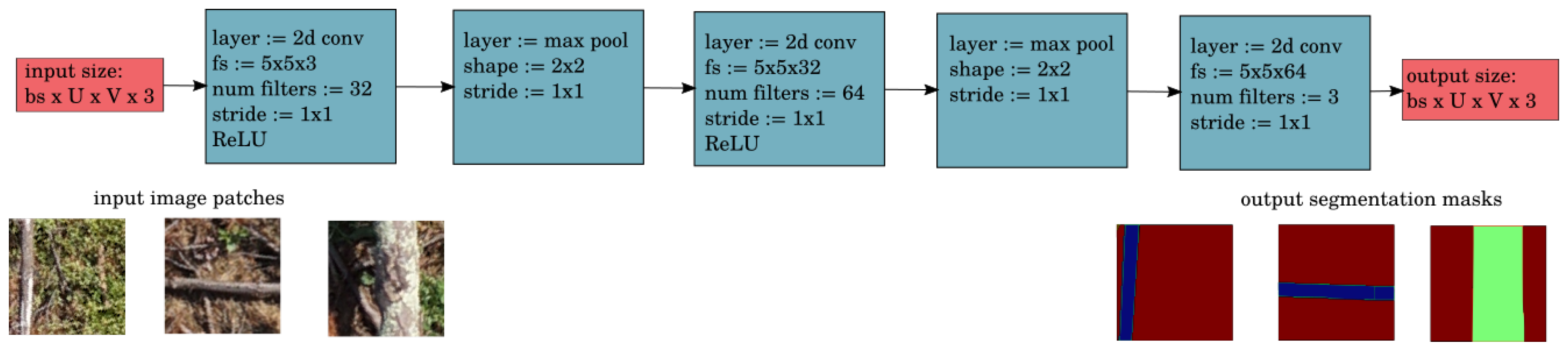
The CNN used for CWD segmentation in this work draws from the FCN, but has some modifications (
Figure 5). Firstly, it only has three layers. This was found to be adequate for the given segmentation task and far more computationally efficient. Secondly, it has no downsampling of the image and no loss in spatial resolution, and hence, finer predictions can be made. Fine-scale predictions are necessary for accurate volumetric estimation. The trade-off for this is a smaller receptive field, but this was found to be sufficient as images were acquired from a high altitude and the logs did not require a large context to distinguish them from the FWD and background classes.
The architecture of the CNN used for segmentation consists of three convolutional layers. The first layer has 32,
filters, the second layer has 64,
filters and the third layer has three,
filters. Each convolutional layer is followed by a ReLU layer [
31] and a
max pooling layer. There are no fully connected layers, so the output is an image with the same dimensions as the input, where each channel is a map of scores for one class (CWD, FWD, and background).
As in FCN, a per-pixel SoftMax function is applied at the output of the final convolutional layer. This function normalizes the output of the network to appear similar to one-hot class labels, which are binary vectors with a one at the class of the datum and zeroes at all other classes. During training, the output of each SoftMax function is compared with one-hot class labels using the standard cross-entropy loss function to optimize the network. The training parameters used for the segmentation CNN are given in
Table 1. For predictions during inference, the index of the maximum across the class axis of the SoftMax layer output is computed for each pixel to get its segmentation label.
An issue with training the CNN is the vast class imbalance. The background class contains many more samples than the CWD and FWD classes. To counteract this, each batch of images used to train the CNN was balanced by weighting the pixels in the loss function so that each class contributed evenly. To make the CNN more generalizable, the images in each batch were also augmented using rotations and flips. This increases the training set size and makes the CNN more robust to this type of variation in the data.
The segmentation CNN does not have fixed input dimensions, so unlike Faster-RCNN the image size during inference can be different to the image size during training. However, there is a computational limitation on the size of images which can be passed through the network. Hence, for computational efficiency, the CNN is trained on images (where the third dimension is the RGB channels), and a sliding window is input into the CNN during inference. Because the segmentation is per pixel, no overlap is required for the sliding window. Hence, its stride for inference is 1000 pixels.
2.4.4. Rectangle Fitting and Refinement
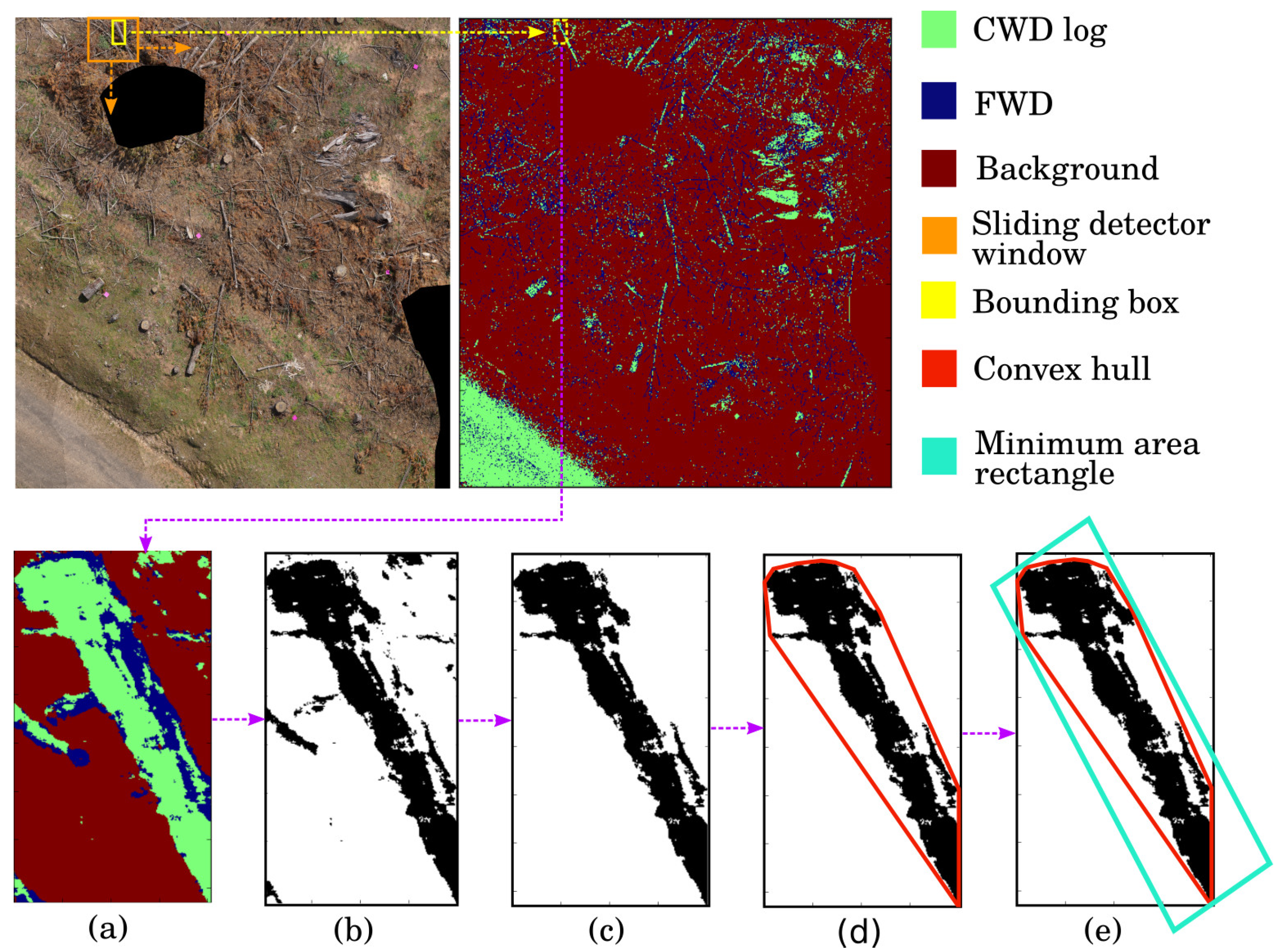
Once the Faster-RCNN log detector and segmentation CNN models are trained, they are applied to the plot mosaic to output a set of bounding boxes containing CWD and a segmented mosaic, respectively. The resulting bounding boxes are axis aligned in the north-east directions; additional processing steps were required to estimate the length and diameter of each log (via rectangle fitting) to calculate volume. The coordinates of a given bounding box are used to extract an image from the segmented mosaic (
Figure 6a). This segmented sub-image is binarized so that CWD pixels have one value and the background and FWD pixels (including branches from logs) have another value (
Figure 6b). Connected components within the binarized sub-image are found, and any components with fewer than 1000 connected pixels are removed as they are likely to be false positives (
Figure 6c). A convex hull is fitted around all remaining components in the sub-image (
Figure 6d), and the rectangle with the smallest area is fitted around the convex hull (
Figure 6e). The result of this process is a rectangle of known dimensions fitted roughly around each detected log.
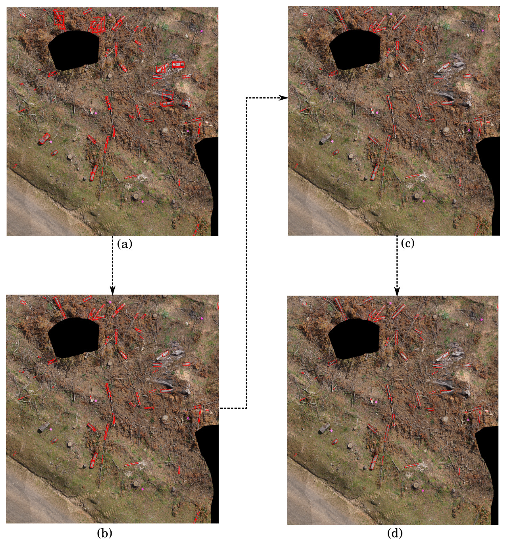
This is followed by a refinement process of the rectangles, where non-realistic rectangles are discarded. As logs should be rectangular rather than square, any rectangles that are too square or unreasonably large are removed (
Figure 7b). The former is achieved by removing any rectangle with an aspect ratio close to 1 (greater than 0.8 and less than 1.2). The latter is done by removing any rectangle whose smallest side is larger than 140 pixels (47.5 cm), since logs are expected to have at least one short side (corresponding to their diameter if they are assumed to be cylindrical).
The size of many of the logs exceeds that of an image which can be passed into the log detector. Hence, it is common to have several overlapping bounding boxes spanning a single log. Due to the overlapping bounding boxes, there should be many overlapping rectangles. To unify them, similar rectangles are grouped together (
Figure 7c), where similarity is characterized by how close their centers and angular orientations are within some tolerance. Two rectangles that belong to the same log should be close together (within 150 pixels) and should be oriented in a similar direction (rotational disparity within 10 degrees). The grouping is done by first seeding a group with a similar pair of rectangles and then subsequently adding a new rectangle if it is similar to any rectangle in the group. New groups are seeded if a similar pair is dissimilar to any other group. Two entire groups can also be merged together if they contain similar rectangles. The more the bounding boxes overlap, the easier the grouping process is. Once this process of grouping is complete, each group of similar rectangles is merged into one meta rectangle by fitting a convex hull around the corner points of all rectangles in the group, and then finding the rectangle of minimum area that fits this convex hull.
After merging, if there is a sufficient amount of overlap between resulting rectangles (greater than 0.75% of the smaller rectangle), this is likely due to two distinctly similar groups of rectangles that correspond to the same rectangle, often resulting in a smaller rectangle within a larger one. In this case, the rectangle with the smaller area is removed (
Figure 7d). Finally, abnormally large rectangles resulting from the merging process (those with no side shorter than 300 pixels i.e., 101.7 cm) are removed. The diameter threshold for removing large rectangles in this step should be higher than for the previous large rectangle removal step. This is because of the possibility of merged rectangles being fitted to logs that are slightly curved or bent such that their apparent diameter is larger. The remaining rectangles should each correspond to distinct logs, and their width and height should align with the length and diameter of the logs. Once a rectangle has been fitted to each CWD log, its volume can be estimated using Equation (
1).
2.5. Implementation Details
Image processing routines were carried out on a 64-bit computer with an Intel Core i7-7700K Quad Core CPU @ 4.20GHz processor and Nvidia GeForce GTX 1080Ti 11GB graphics card. The deep learning framework used was Tensor Flow version 1.4.1 (in python).
2.6. Training Data for Automated Detection/Segmentation Algorithms
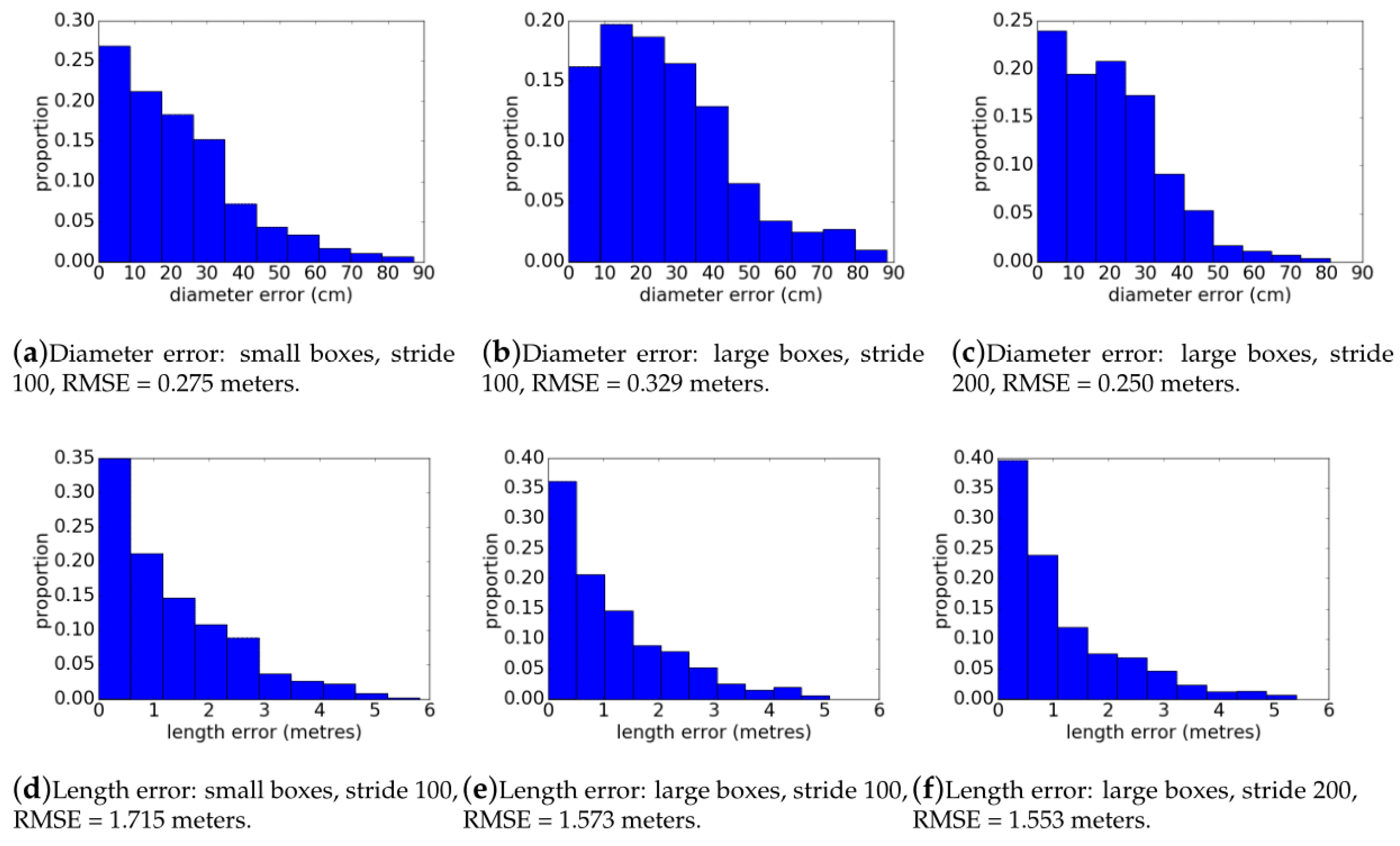
To train the Faster R-CNN detectors, image crops were sampled from each plot and given bounding box annotations. When labelling logs, two annotation styles were used. One set of the annotations covered the entire log visible in each image. Thus, the number of images with log annotations ranged from 10–20 per plot, and bounding box labels were more likely to contain background noise, particularly of the logs were not aligned with the axes of the image crop. This method of training the detector is referred to as ‘large boxes’ in the rest of the paper. The other style used much smaller (the length was capped at the diameter of the log), tighter fitting bounding boxes that were automatically generated from the per-pixel labels. In the case of a large log, several small bounding boxes were used to annotate its different sections. Multiple translated views of the same logs with bounding boxes were also used. Using this method, several hundred images of annotations were generated for each plot. This method of training the detector is referred to as ‘small boxes’ in the rest of the paper. For each plot, 30 additional images, containing solely background classes, were annotated. The background classes comprised stump, grass (weed), patches of bare ground that resembled stumps, marker, and FWD. These were used as negative cases to reduce the number of false positive detections. The detector trained on the ‘large bounding boxes’ was also used as the stump detector in the experiments (as stump was one of the background classes).
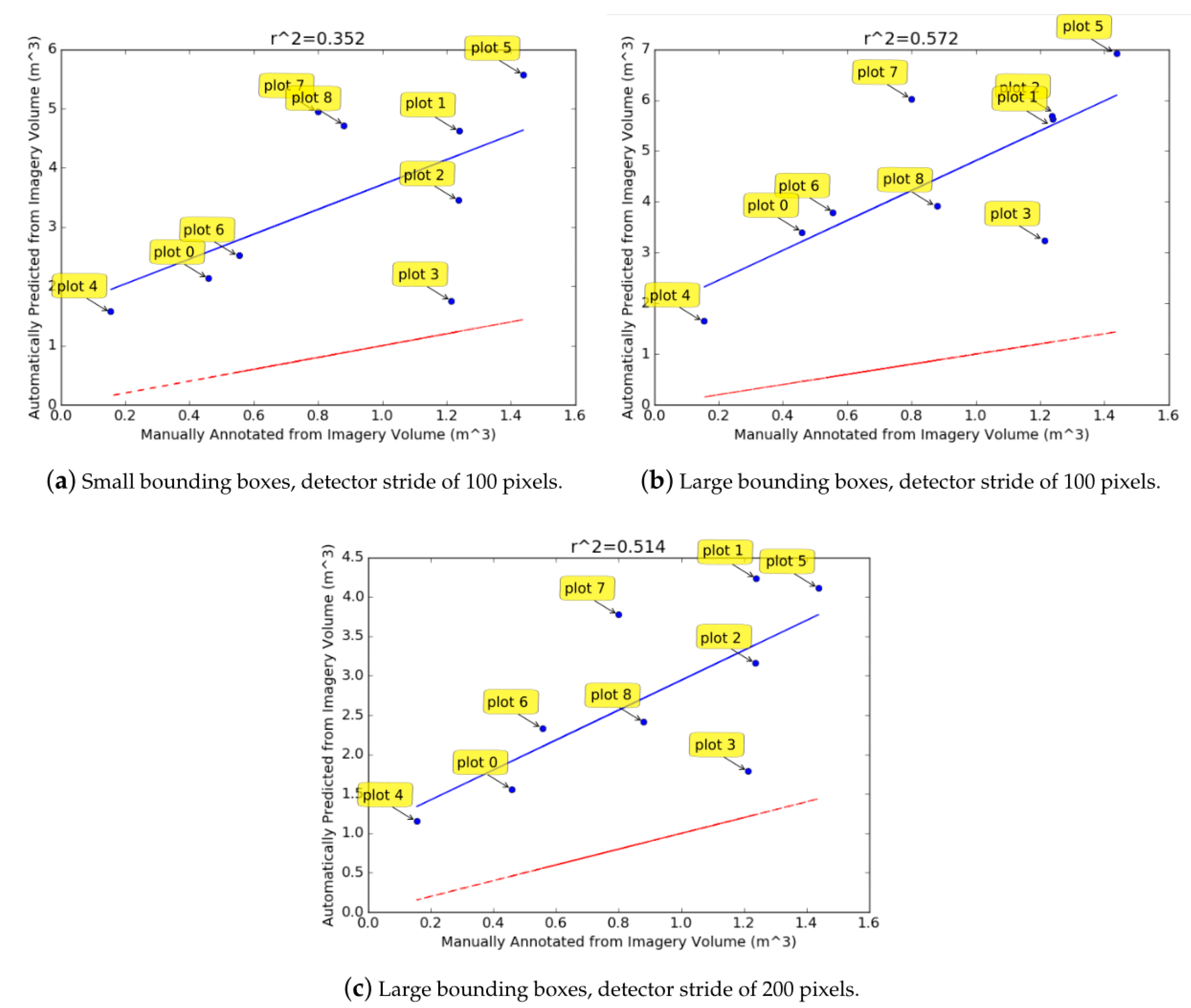
For the CWD detection, three types of detector were trained for the experiments: ‘small boxes, stride 100’, ‘large boxes, stride 100’ and ‘large boxes, stride 200’. The ‘small boxes, stride 100’ detector was trained using the small boxes described above and a stride of 100 pixels in the x and y directions was used for the sliding window in the inference phase. The ‘large boxes, stride 100’ and ‘large boxes, stride 200’ detectors were trained with the large bounding boxes described above. The stride for the detector during inference was 100 and 200 pixels respectively. For the small bounding box case, there were significantly more training examples than for the large bounding box scenario.
For the segmentation CNN, 1000 image crops were randomly sampled from the per-pixel labelled mosaic for each plot. The stump labels were removed, leaving CWD, FWD, and background. Each sampled image crop was .
2.7. Cross-Validation of Automated Stump Detection and CWD Volume Estimation Algorithms
Cross-validation, where the dataset is divided into varying testing and training partitions, was used to validate how well the proposed approach generalized to datasets that it was not trained on. For each fold of the cross-validation, two plots were used for training and seven plots were used for testing. Since there were two distinct background colors in the plots captured by the UAV (
Table 2), the plots were grouped based on this color so that the models trained would be exposed to both backgrounds. Plots 0, 1, 2 and 3 formed the group one and plots 4, 5, 6, 7, and 8 formed group 2. Each fold consists of a combination of one plot from each group. This allows for a maximum of 20 folds (20 possible combinations of plots). From this list of 20 folds, ten folds were selected at random. The combinations of plots for these folds are listed in
Table 3. The Faster-RCNN detector and Segmentation CNN models were trained on data from the plot combinations associated with each fold. Inference using the entire pipeline was then conducted on all other plots. The performance of the pipeline for each plot when trained on each fold was reported in the results.
The motivation behind the autonomous algorithms was to reduce the large manual effort currently required in the field to estimate the volume of CWD and locate stumps. While labelling images for training an autonomous approach is already significantly easier than the usual field work, the number of labelled plots used for training was kept low (two) to further reduce manual effort.
2.8. Evaluation Metrics for Automated Stump/Log Detection
A stump was considered detected if the pixel intersection over union, given by:
between a ground truth bounding box
and predicted bounding box
was greater than
[
32]. Using this measure for correct bounding box detection, the precision and recall for each class was calculated. The precision and recall are given by:
where
are the true positives,
are the false positives and
are the false negative matches with a detection confidence threshold of 0.97.
For the logs, the detection accuracy was determined, as well as the accuracy of the dimensions of the rectangles, as this was critical to estimating the volume. Because it was difficult for a single rectangle to fit an entire log, the detection accuracy was relaxed such that partial log detections were counted as long as the total intersecting area of rectangles and logs for rectangles covering a given log summed to at least of the log area. Thus, recall was the proportion of all logs that had at least half of their area covered by predicted rectangles (such that the result was not skewed by having multiple rectangles on a single log). The precision was the proportion of all predicted rectangles that belonged to a detected log.
From the predicted rectangles that contributed to a log detection, the error in the length and width dimensions of these rectangles was also determined. These were aggregated into histograms over all folds and plots. Error associated with rectangles only fitting to partial logs were captured in these statistics, as rectangles that only fit a partial log have a large error in their length dimension.
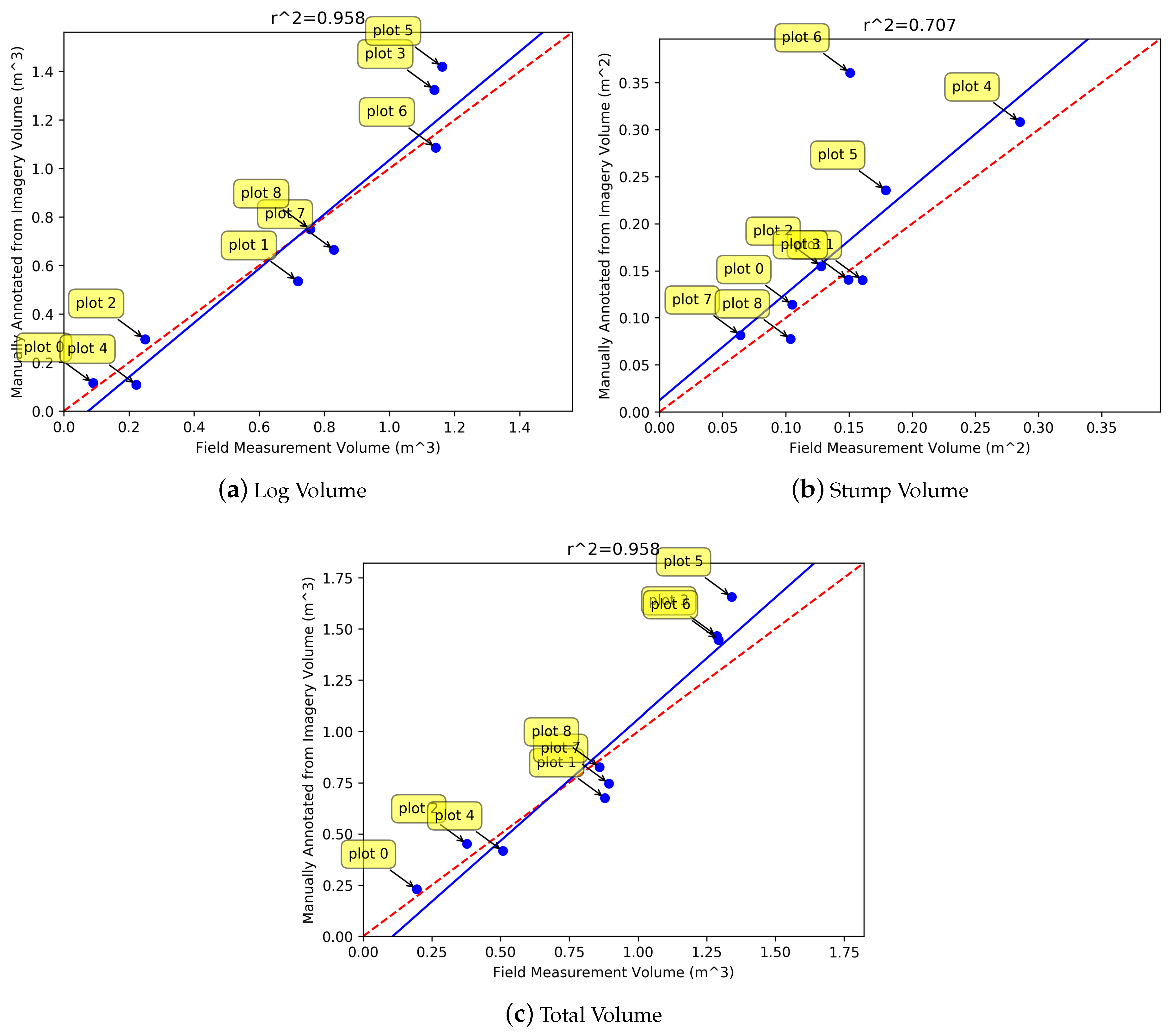
Regression analysis is used to analyze the relationship between the predicted and ground truth plot volume for the different plots, with used to determine the correlation. While the volume predicted from manual annotations of UAV imagery is compared with the volume calculated from the field measurements, the volume predicted from the automated method is compared with the volume predicted from the manual UAV image annotations. There are pieces of CWD that were missed in the UAV manual annotation because they were completely covered by slash, but the objective of the study was to evaluate the automated method in terms of what was visible from the air. A secondary motivation for using the UAV manual annotation as a reference for the automated method is that additional pieces of CWD outside of the marker region could be annotated, increasing the number of samples for the study. This was done for plots 0, 1, and 2, which had few samples in the marked region.
4. Discussion
The recall for the stump detection decreased slightly for the plots with a higher FWD density (
Table 4). In the lower density plots, most of the stumps are clearly visible, where as in the high-density plots some of the stumps are occluded by debris and only partially visible from above. Faster-RCNN is successful in detecting many of these partially visible stumps. However, for the cross-validation folds where it has not been trained on many partially occluded stumps, the recall is lower.
The issue of occlusion is also a challenge for the log rectangle fitting. From the results of
Table 5, the recall is low for plot 8 where the density of the debris is highest. Many of the logs in
Figure 9b are only partially fitted with rectangles as part of their length is occluded. If rectangles are fitted to two parts of the same log, separated by some occluding debris, then they will not be merged together if the centers of the rectangles exceed the 150-pixel merging threshold. If, however, this threshold is increased to allow logs with large occlusions to be merged, then more logs with similar rotations within the greater radius will be incorrectly merged, most likely resulting in the rectangle being discarded. This was determined to be more problematic than missing the volume of the occluded section of the log.
For both the stump detection and the log rectangle fitting, the trainable CNN components for detection and segmentation generalize well to unseen data. In the cross-validation results for the precision and recall, for a given fold, the performance on a training plot was typically only slightly higher than the performance on a validation plot.
There was some variation in the results across different folds. For example, the stump detector from folds 2 and 3 has poor performance overall in comparison to the other folds. This could be related to the data used for training. Training examples from plot 6 were used for both folds 2 and 3, suggesting that these examples could either have been inaccurately annotated or were not a good representation of a typical plot, such that the models they were used to train did not generalize well to the other scenes. Given that the performance on plot 6 was high for both folds 2 and 3, it is most likely to be the latter. For the log rectangle fitting, performance was particularly bad for fold 2. This is also likely attributed to plot 6 having non-representative training examples, as the performance is high on plot 6 but low for many of the other plots. It could also be related to the examples in plot 2 (which was the other plot used to train fold 2). The precision and recall of the rectangles are both low for plot 2 fold 2, suggesting that the label related labels themselves for this plot were poorly annotated. However, given the small number of plots it is difficult to draw definitive conclusions.
In comparison to other works, the use of a CNN-based approach demonstrated a strong improvement over more traditional methods. Using the region-growing approach, Puliti et al. [
17] had difficulty in differentiating stumps and log residuals. With adequate training examples, a CNN-based approach learns the features it requires to distinguish these classes despite their similar appearance. In trying to fit circles to detect stumps, Samiappan et al. [
18] discusses how the stumps in their dataset are actually imperfect ovals rather than circles, reducing detection accuracy. A CNN-based approach is trained to be robust to small variations in the data such as this. The high-resolution imagery was also advantageous for stump detection. Samiappan et al. [
18] suffered from degraded performance due to the resolution of the imagery as shape boundaries were difficult to delineate. The resolution of Puliti et al. [
17] resulted in stumps with relatively small diameters frequently being missed.
The variance in the results of
Table 5 and of
Figure 10 across methods are linked to how the Faster-RCNN object detector component is trained. When smaller boxes are trained on, the precision score is lower. Low precision indicates too many detections are being made, resulting in a high number of false positives. Objects such as FWD that look similar to CWD are being incorrectly predicted as logs. This can be explained by the bounding boxes seeing less of the log, and hence having a more limited overall view of what a log is. When larger bounding boxes are used for training, the precision is higher. However, with larger bounding boxes being predicted, there is an increased likelihood of additional CWD logs also being inside the box. As a result, the convex hull is fit around the additional logs (see
Figure 6e), and the rectangle that is fit has inaccurate dimensions. This is reflected in the higher diameter error of the predicted rectangles, which causes the histograms of
Figure 10a,b to be more skewed towards the higher error, (this effect is the cause of some of the wider rectangles in
Figure 9b, where there are many logs overlapping with one another). When the larger stride is used for the sliding window, fewer bounding boxes are predicted and this skews the distribution of diameter errors slightly towards lower error (i.e., lower RMSE). There is a noticeable reduction in the number of predicted rectangles with a diameter error of greater than 50 cm. This training strategy does however result in a slightly poorer recall. This is evident in
Figure 6, where some logs that appear obvious have been missed. This is likely to be related to the fewer detections found due to the larger stride. Some logs might not be detected properly if they do not have a favorable translation in the sliding window, and with fewer sliding windows this becomes more prevalent. This method has the highest overall precision of the three approaches.
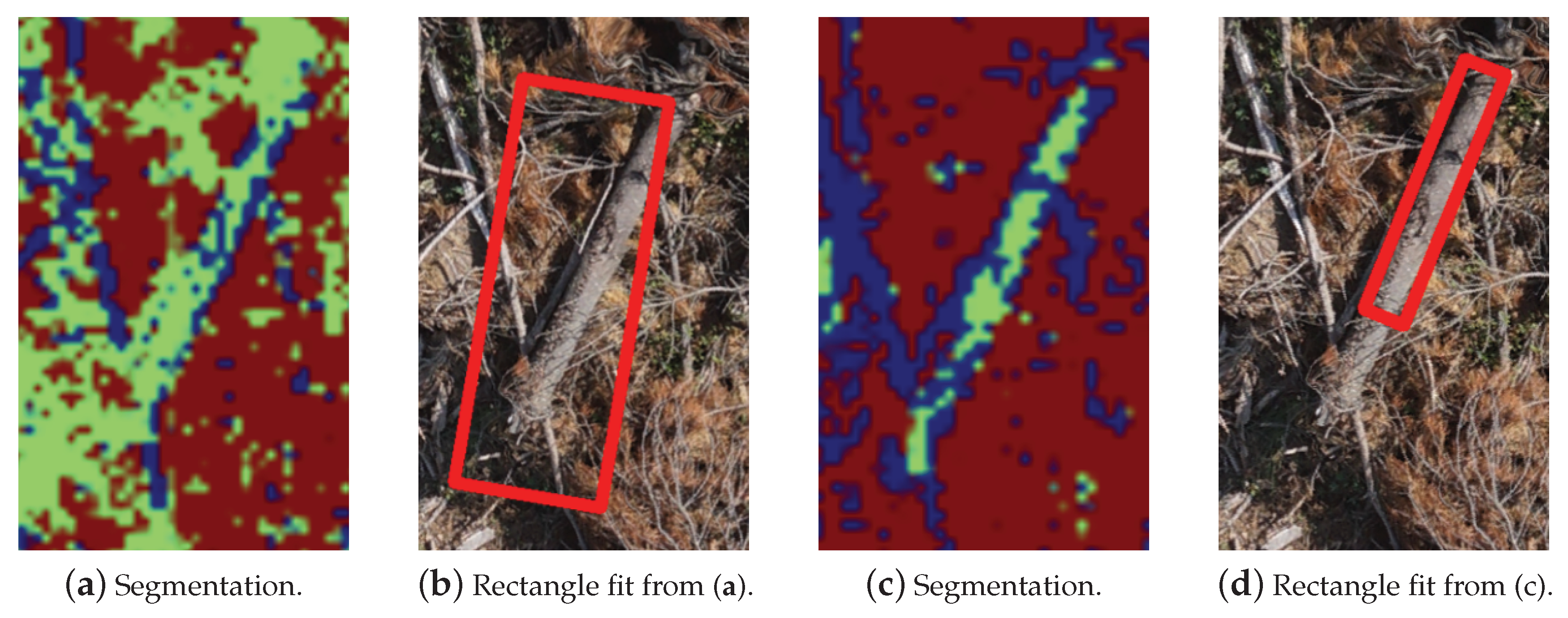
The segmentation is critical for the accuracy of the rectangle fitting step. The CNN must classify the pixels corresponding to the fine branches attached to a log as FWD, not CWD. Otherwise the convex hull will fit around the branches and the shorter length of the fitted rectangle will be an overestimate of the diameter of the CWD log. An example of this is seen in
Figure 15. The segmentation model that results in
Figure 15a labels much of the pixels corresponding to FWD in the background as CWD, and the resulting rectangle in
Figure 15b is poorly fitted to the CWD. However, the segmentation model that produces
Figure 15c appropriately labels FWD and background pixels, so that the fit around the CWD is much tighter (
Figure 15d), although still not perfect as it has labelled some of the CWD pixels as FWD.
The results in
Figure 9 show that some of the fitted rectangles are overlapping slightly even after the refinement step. This indicates that when merging, there were at least two distinct groups of rectangles and the overlap of the resulting merged rectangles is less than the threshold. The threshold cannot be lowered, or else intersecting logs will not be fitted with rectangles. Also, if the merging thresholds are relaxed, then the rectangles fitting to nearby logs will be merged.
The reason for the rectangle fitting having a lower overall recall than the stump detection is because of the additional steps on top of detection that are required for rectangle fitting. Rectangles around logs can be discarded if they become excessively large due to poor merging in the refinement step or nearby logs corrupting the convex hull before rectangle fitting occurs. The precision is also lower because the log detection is harder than the stump detection as it must differentiate between the sometimes very similar CWD and FWD. This results in many false positives, which is especially the case when training on smaller bounding boxes.
The
values for the volume estimation results (
Figure 12) suggest that there is a correlation (although weak) between the automatically predicted volumes and the volume calculated from the manual annotations. However, the predicted volumes are consistently larger than those found from manual annotations. This is likely to be because most rectangles overestimate the diameter of the CWD logs due to errors accumulating in the convex hull and merging phases of the pipeline (e.g.,
Figure 10b there is a large proportion of diameters with an error of 10–40 cm). The over-estimation of the diameter can be observed in the
Figure 9 results. Since the volume of a cylinder is proportional to the square of the diameter, any errors in the diameter estimation have large repercussions for the volume estimation. The weakly correlated prediction and manually annotated volumes indicates that the over-estimation of log diameters is fairly consistent. By observing the errors in
Figure 10a–c, and considering the typical diameter of CWD logs, it was empirically deduced that the logs estimated in the results of
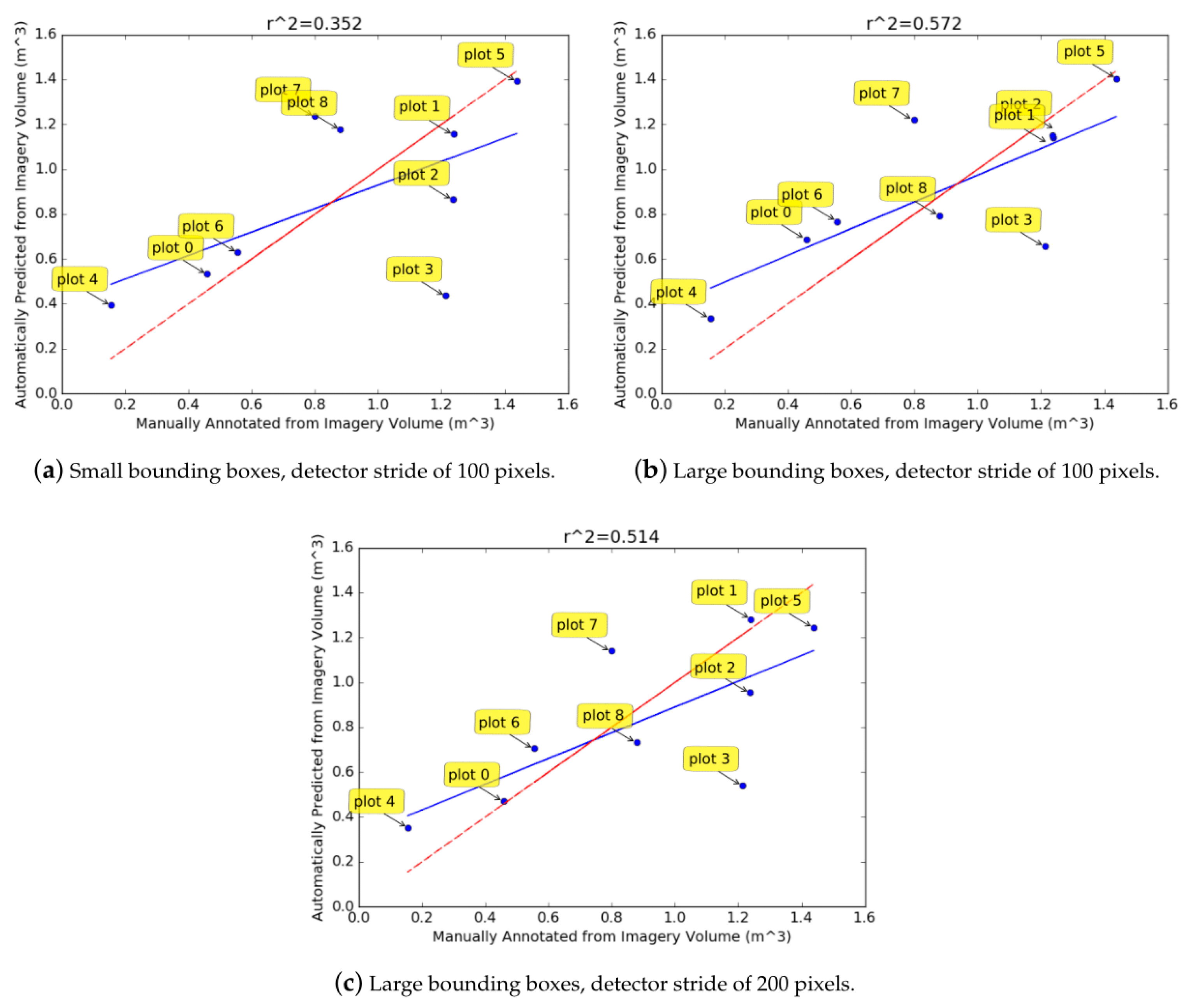
Figure 12 were about 45–55% too large. When the diameter of all rectangles was reduced to account for this over-estimation and the volumes were re-calculated (
Figure 13), the regressed blue line was closer to the red line which indicates that the predicted volumes were more accurate. Scaling the diameter does not change the correlation value, as all logs for a given method are scaled uniformly. The scaling attempts to correct the consistent over-estimation of the diameters.
The remaining lack of correlation of the predictions and ground truth could be attributed to the detections not having a perfect precision and recall, as well additional error variation in the diameter and length estimates of the logs. Plot 7 has a high error in
Figure 13a–c. Its density could be a factor contributing to this, as greater density results in more errors when fitting the convex hull (explained previously). Because of the small number of plots, the correlation result is very sensitive to any relatively large deviations from the regression line (such as plots 3 and 7).
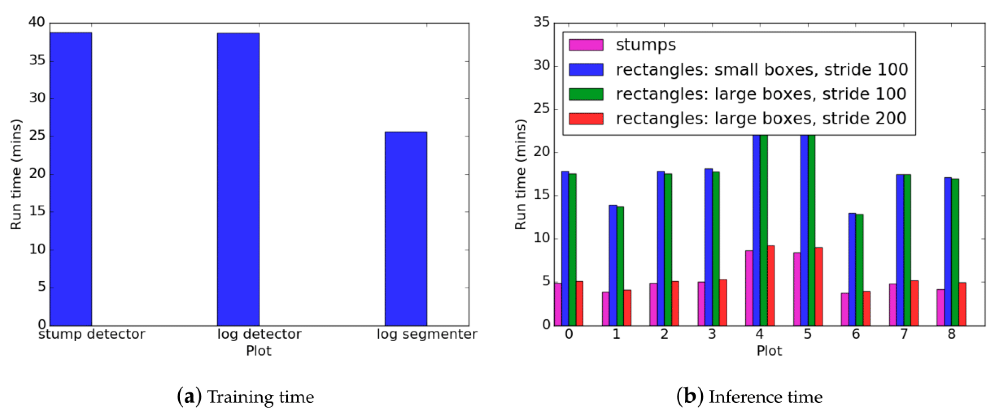
The results of
Figure 14 are typical from a machine learning pipeline in that training time is higher than inference. The inference phase is usually significantly faster than the training time (in the order of seconds). In this case, it took several minutes for inference to occur on a single plot. This is due to the object detection which must be run once for each sliding window. Since the sliding window has a small stride (100 pixels for the stumps, and 100–200 pixels for the logs), the object detector is run hundreds to thousands of times. This explains why having the stride of 200 pixels is significantly faster than the stride of 100 pixels for the rectangle fitting of logs. The rectangle fitting inference was also slightly longer than the stump detection inference despite the stride being the same. This is because of the additional segmentation and computational geometry steps. However, the extra time required for these steps is marginal due to the segmentation algorithm having a much larger stride (1000 pixels) and hence a faster inference in comparison to the object detector. Training time for the segmentation network was also faster than the object detector because the network has fewer parameters.
In comparison to the UAV-borne work of [
16], the CWD log volume estimation of this work was able to adapt to variations in the background better. Davis [
16] relies on the red channel of the image to differentiate the debris from the ground. However, this method is not robust to different backgrounds as was noted when there was flooding, causing the volumetric estimation performance to decrease. The CNN-based log segmentation and detection models in this work are trained on different background to instill invariance. Davis [
16] uses a traditional computer vision approach, the mean-shift algorithm, to estimate a debris mask. It cannot differentiate between the coarse and fine pieces of debris, which is necessary for volumetric estimation, resulting in over-estimates of the volume that are larger than those of this study. The CNN-based segmentation model in this paper is trained to segment coarse and fine debris separately.
5. Conclusions
Using a sample size of nine plots, the results indicated that the use of UAV-derived, high-resolution imagery and digital annotation of the imagery provided an alternative to in situ, field-based manual measurements (calipers and tape measure), with equivalent measurement results, and hence accuracy. Differences were due to several factors: not all timber was visible from the air, as in some quadrats large pieces of debris lay underneath other branches and pine needle foliage, making it difficult to discern from the air. Although stump areas corresponded well ( = 0.971), the correspondence between stump heights measured in the field vs. those extracted from digital surface models was poor ( = 0.374). This was owing to several factors including the fact that the digital surface model sometimes only provided measurements of material elevation (rather than ground elevation) because of clutter such as debris and slash.
Automated algorithms were able to effectively detect stumps and results showed that stems could be detected on average with a precision of 83.9% and a recall of 81.8%. They were also able to distinguish between different size classes of debris (CWD versus FWD) to estimate the volume of CWD, but with worse accuracy than the manually annotated imagery. However, once the detection and segmentation models were trained, the automated approach required significantly less effort than the manual, digital annotation.
The traditional in situ measuring method had the advantages of requiring minimal equipment (calipers and tape measure) but took more time in the field and more personnel. The UAV imagery-based methods for manual and autonomous annotation took less time in the field for both setup and data collection, but required specialized equipment (a UAV) and specialized/trained personnel to operate the UAV (remote aircraft pilot for takeoff/landing). Both the in situ and manual imagery-based annotation method took approximately the same amount of time in post-fieldwork activities/analysis. Both of these methods provided essentially equivalent results in terms of quantifying woody debris volume on the ground; however, it should be noted that the ability to quantify debris from the air was dependent on the amount of occlusion owing to slash and pine needle foliage present at the site. The biases introduced by these types of occlusions are a limitation for remote sensing approaches. The autonomous imagery-based method required less time in post-fieldwork activities/analysis at the expense of accuracy. The capacity to collect more data while taking less time in the field using the UAV imagery-derived estimates, provides the advantage that a larger sample size of post-harvest debris could be collected, giving a potentially better representation of the actual debris quantity over a full harvested compartment. This would obviously require more time for post-fieldwork analysis.
In addition to the quantification of woody debris, our method provides a map of detected stumps. One potential use of this stem map is in validating stocking estimates (number of trees per hectare) made during pre-harvest inventories, for example by LiDAR-based imputation, that use individual tree detection methods. If post-harvest stem maps can be correlated with pre-harvest stem maps generated from LiDAR, this has the potential to assist in the refinement of imputation models for future inventory activities.
An improved method of estimating post-harvest residues may greatly assist in the assessment of the feasibility of extraction of that resource for applications such as bioenergy - as currently significant volumes of pine plantation harvest residues are under-used [
33]. Their estimation is also useful for maintaining the quality of a site, and can be used to reconcile differences between pre-harvest estimates of timber yield and actual timber yield. For future work, the autonomous algorithm could potentially be made more accurate by incorporating information from the digital surface model derived using structure from motion and photogrammetry. The surface model captures variations in the height owing to larger logs and could also provide queues to segmenting different ground cover types owing to the structural texture present. The surface model can be converted into a rasterized grayscale image layer that could be added to the existing color image layers and provided as part of the input data to the image-based machine learning algorithms presented here. Future work will also consider the use of UAV-borne imagery for characterizing post-harvest site variables such as access roads and skid trails.


