Application of A Simple Landsat-MODIS Fusion Model to Estimate Evapotranspiration over A Heterogeneous Sparse Vegetation Region


Abstract
:
1. Introduction
2. Materials and Methods
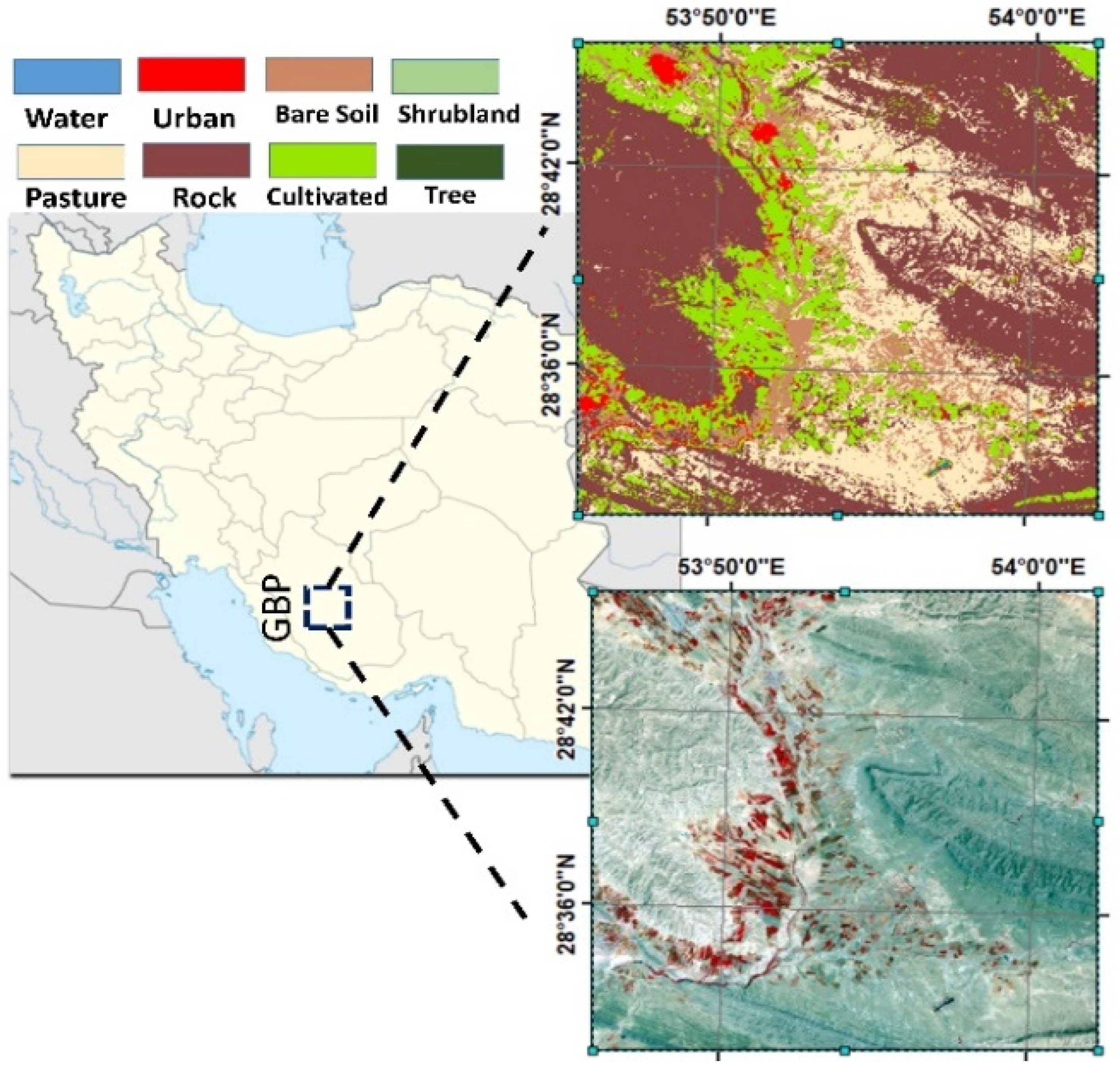
2.1. Study Site
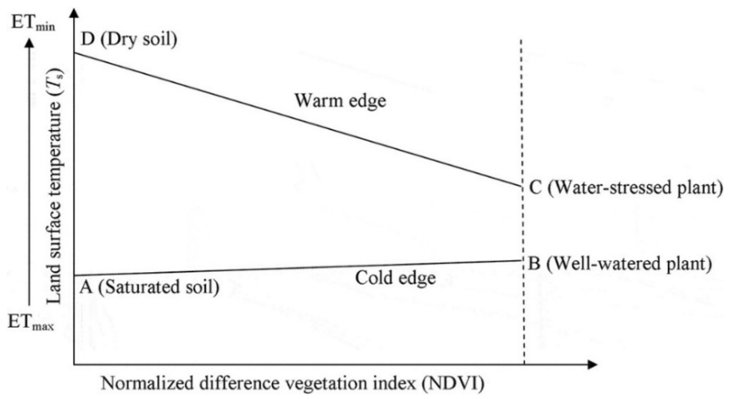
2.2. The METRIC Algorithm
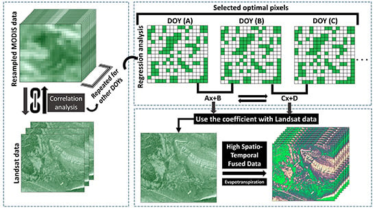
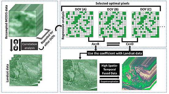
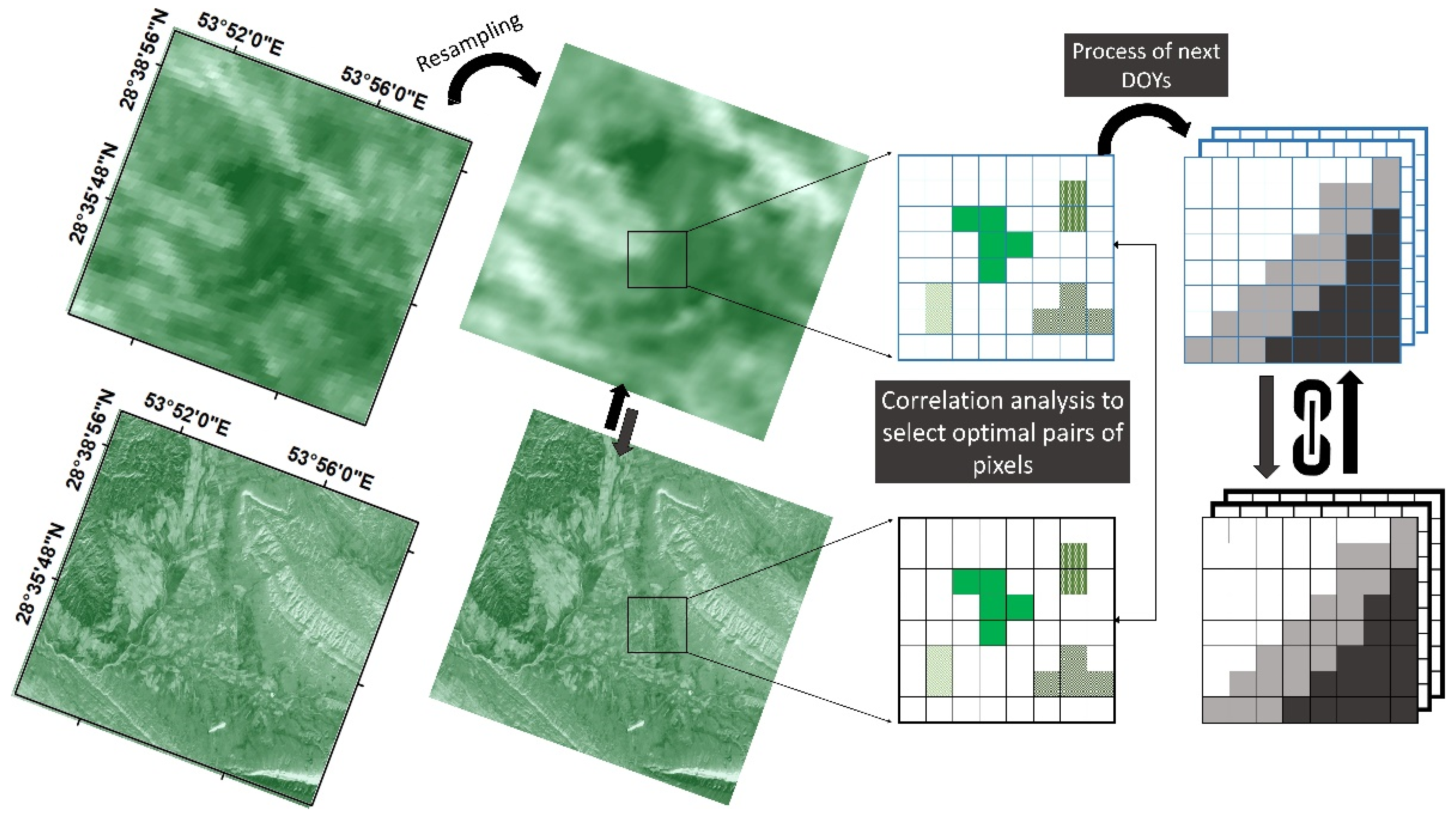
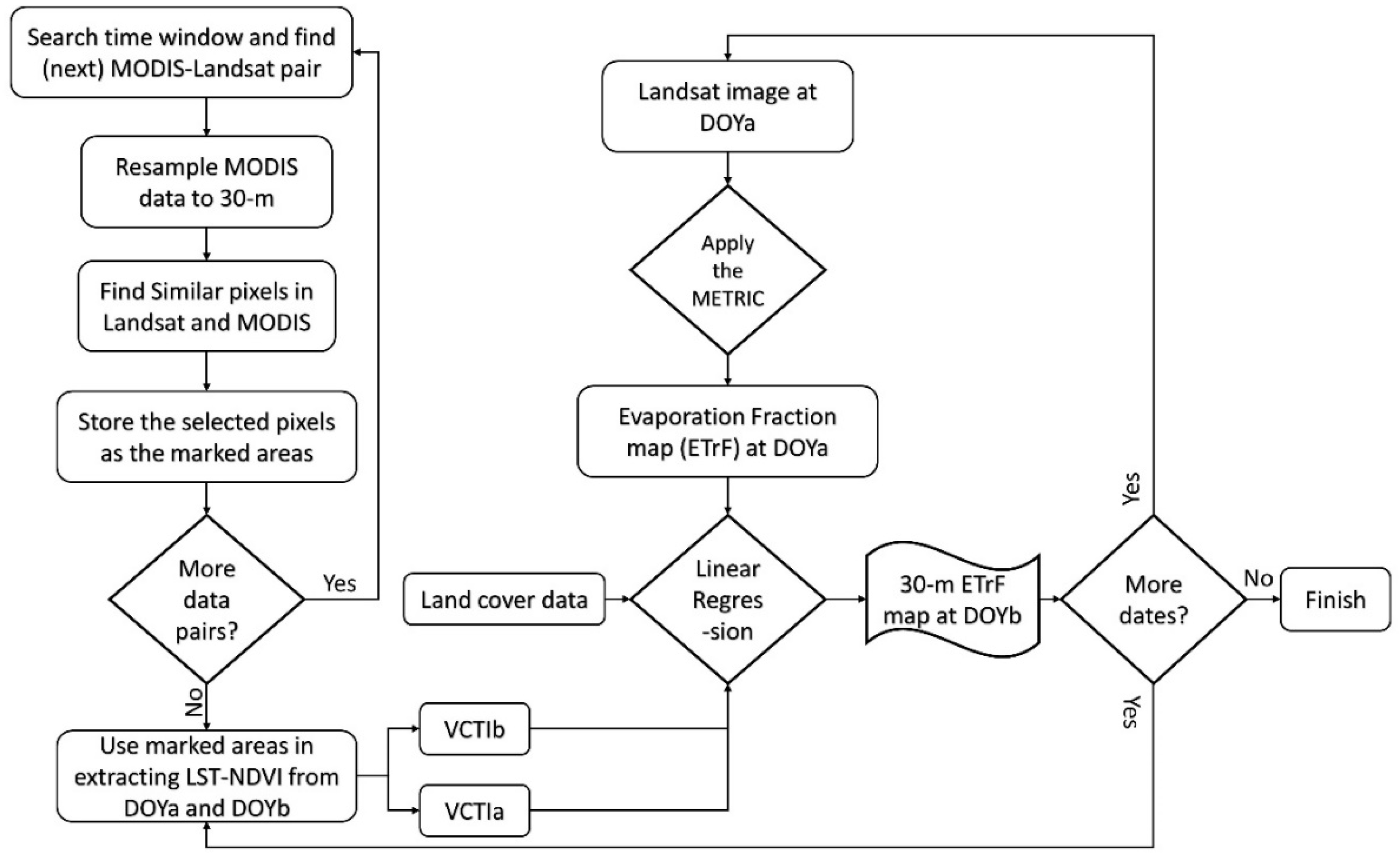
2.3. The MODIS–Landsat Fusion Model
2.4. Modifications to the Fusion Model
2.5. Frequency Update Experiments
2.6. Data and Model Evaluation
2.6.1. Data
2.6.2. Model Evaluation
3. Results and Discussion
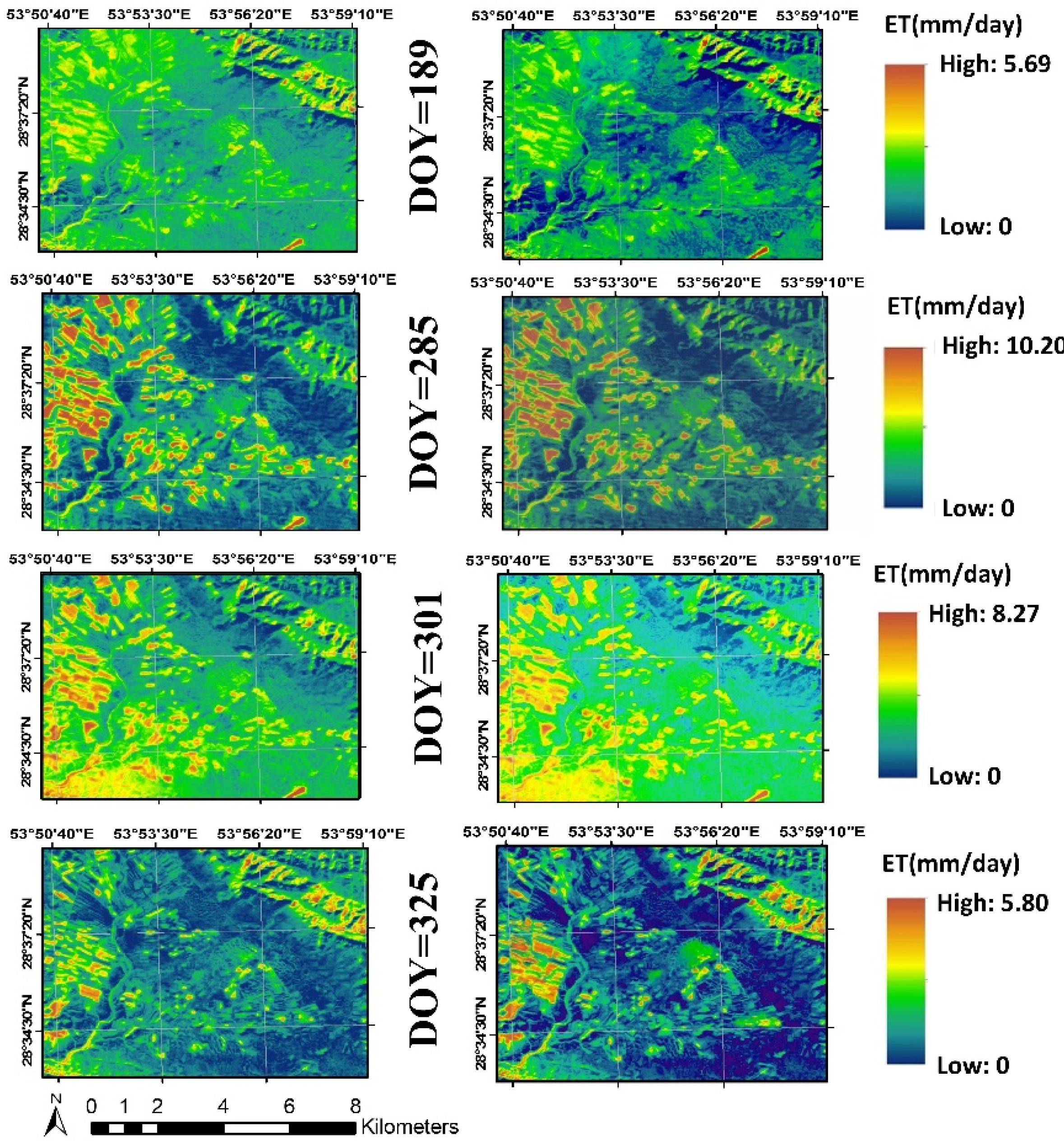
3.1. Initial Results with the Original and Modified Models
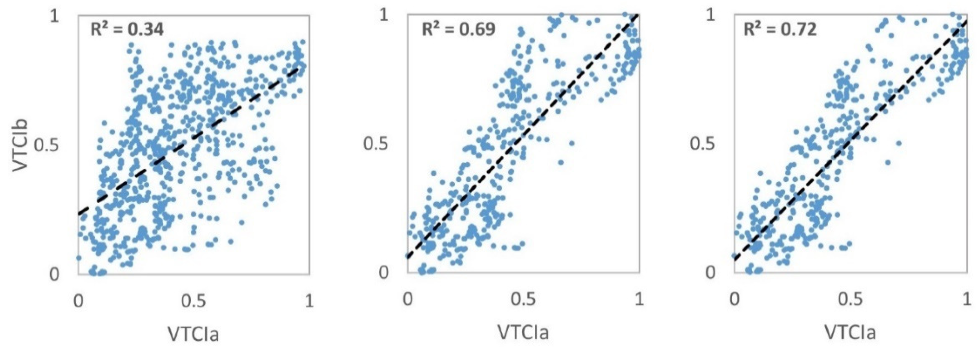
3.2. Pixel Level Evaluation Results
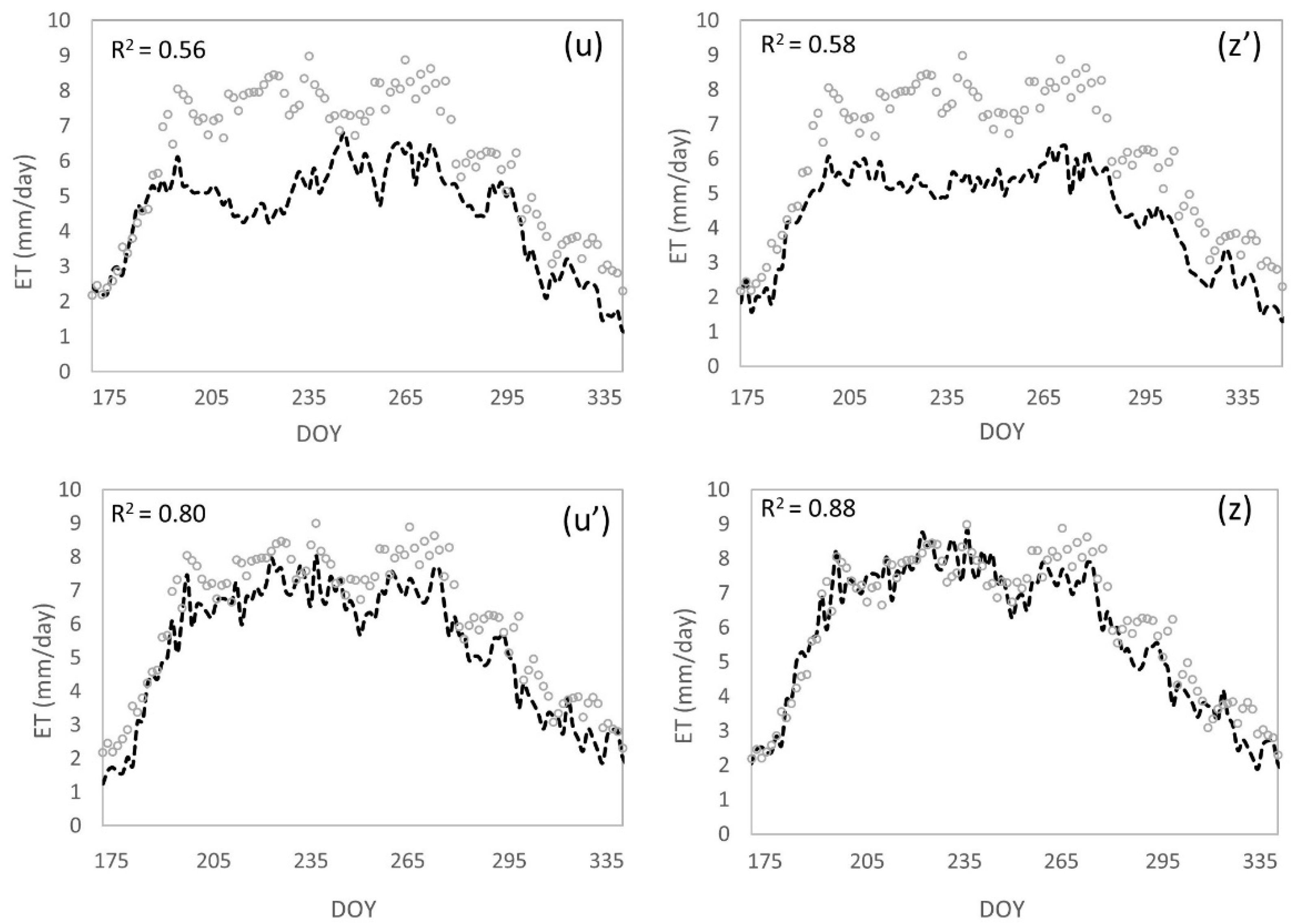
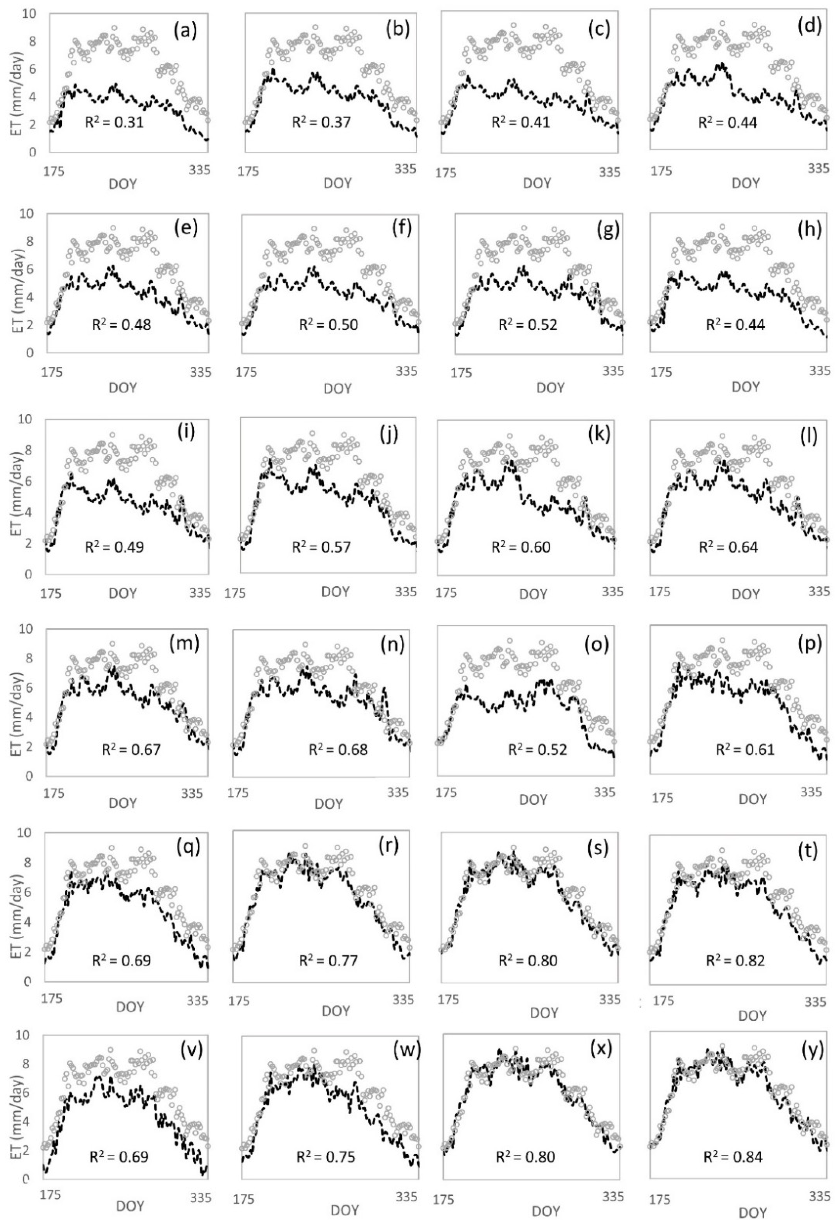
3.3. Effects of Data Update Frequency on the Fusion Model
3.4. Comparison at the Watershed Level
4. Conclusions
Author Contributions
Funding
Acknowledgments
Conflicts of Interest
References
- Tilman, D.; Cassman, K.G.; Matson, P.A.; Naylor, R.; Polasky, S. Agricultural sustainability and intensive production practices. Nature 2002, 418, 671–677. [Google Scholar] [CrossRef] [Green Version]
- Tabari, H.; Talaee, P.H. Temporal variability of precipitation over Iran: 1966–2005. J. Hydrol. 2011, 396, 313–320. [Google Scholar] [CrossRef]
- Bastiaanssen, W.G.M.; Menenti, M.; Feddes, R.A.; Holtslag, A.A.M. A remote sensing surface energy balance algorithm for land (SEBAL). 1. Formulation. J. Hydrol. 1998, 212, 198–212. [Google Scholar] [CrossRef] [Green Version]
- Su, Z. The Surface Energy Balance System (SEBS) for estimation of turbulent heat fluxes. Hydrol. Earth Syst. Sci. 2002, 6, 85–100. [Google Scholar] [CrossRef] [Green Version]
- Allen, R.G.; Tasumi, M.; Trezza, R. Satellite-based energy balance for mapping evapotranspiration with internalized calibration (METRIC)—Model. J. Irrig. Drain. Eng. 2007, 133, 380–394. [Google Scholar] [CrossRef]
- Irmak, S.; Kabenge, I.; Rudnick, D.; Knezevic, S.; Woodward, D.; Moravek, M. Evapotranspiration crop coefficients for mixed riparian plant community and transpiration crop coefficients for Common reed, Cottonwood and Peach-leaf willow in the Platte River Basin, Nebraska-USA. J. Hydrol. 2013, 481, 177–190. [Google Scholar] [CrossRef]
- Trezza, R.; Allen, R.; Tasumi, M. Estimation of actual evapotranspiration along the Middle Rio Grande of New Mexico using MODIS and landsat imagery with the METRIC model. Remote Sens. 2013, 5, 5397–5423. [Google Scholar] [CrossRef]
- French, A.N.; Hunsaker, D.J.; Thorp, K.R. Remote sensing of evapotranspiration over cotton using the TSEB and METRIC energy balance models. Remote Sens. Environ. 2015, 158, 281–294. [Google Scholar] [CrossRef]
- Wagle, P.; Bhattarai, N.; Gowda, P.H.; Kakani, V.G. Performance of five surface energy balance models for estimating daily evapotranspiration in high biomass sorghum. ISPRS J. Photogramm. Remote Sens. 2017, 128, 192–203. [Google Scholar] [CrossRef]
- Jamshidi, S.; Zand-Parsa, S.; Pakparvar, M.; Niyogi, D. Evaluation of Evapotranspiration over a Semi-Arid Region using Multi-Resolution Data Sources. J. Hydrometeorol. 2019. [Google Scholar] [CrossRef]
- Thoreson, B.; Clark, B.; Soppe, R.; Keller, A.; Bastiaanssen, W.; Eckhardt, J. Comparison of evapotranspiration estimates from remote sensing (SEBAL), water balance, and crop coefficient approaches. In Proceedings of the World Environmental and Water Resources Congress 2009: Great Rivers, Kansas City, MI, USA, 17–21 May 2009; pp. 1–15. [Google Scholar] [CrossRef]
- Mkhwanazi, M.M.; Chávez, J.L. SEBAL-A: A Remote Sensing ET Algorithm that Accounts for Advection with Limited Data. Part I: Development and Validation. Hydrol. Days 2015, 7, 15046–15067. [Google Scholar] [CrossRef] [Green Version]
- Gowda, P.; Chávez, J.; Howell, T.; Marek, T.; New, L. Surface energy balance based evapotranspiration mapping in the Texas high plains. Sensors 2008, 8, 5186–5201. [Google Scholar] [CrossRef] [PubMed]
- Lian, J.; Huang, M. Evapotranspiration estimation for an oasis area in the Heihe River Basin using Landsat-8 images and the METRIC model. Water Resour. Manag. 2015, 29, 5157–5170. [Google Scholar] [CrossRef]
- Semmens, K.A.; Anderson, M.C.; Kustas, W.P.; Gao, F.; Alfieri, J.G.; McKee, L.; Prueger, J.H.; Hain, C.R.; Cammalleri, C.; Yang, Y. Monitoring daily evapotranspiration over two California vineyards using Landsat 8 in a multi-sensor data fusion approach. Remote Sens. Environ. 2016, 185, 155–170. [Google Scholar] [CrossRef] [Green Version]
- Carper, W.; Lillesand, T.; Kiefer, R. The use of intensity-hue-saturation transformations for merging SPOT panchromatic and multispectral image data. Photogramm. Eng. Remote Sens. 1990, 56, 459–467. [Google Scholar]
- Shettigara, V.K. A generalized component substitution technique for spatial enhancement of multispectral images using a higher resolution data set. Photogram. Enggineer. Remote Sens. 1992, 58, 561–567. [Google Scholar]
- Yocky, D.A. Multiresolution wavelet decomposition I me merger of landsat thematic mapper and SPOT panchromatic data. Photogramm. Eng. Remote Sens. 1996, 62, 1067–1074. [Google Scholar]
- Pohl, C.; Van Genderen, J.L. Review article multisensor image fusion in remote sensing: Concepts, methods and applications. Int. J. Remote Sens. 1998, 19, 823–854. [Google Scholar] [CrossRef]
- Zhang, Y. Understanding image fusion. Photogramm. Eng. Remote Sens. 2004, 70, 657–661. [Google Scholar]
- Thomas, C.; Ranchin, T.; Wald, L.; Chanussot, J. Synthesis of multispectral images to high spatial resolution: A critical review of fusion methods based on remote sensing physics. IEEE Trans. Geosci. Remote Sens. 2008, 46, 1301–1312. [Google Scholar] [CrossRef]
- Gao, F.; Masek, J.; Schwaller, M.; Hall, F. On the blending of the Landsat and MODIS surface reflectance: Predicting daily Landsat surface reflectance. IEEE Trans. Geosci. Remote Sens. 2006, 44, 2207–2218. [Google Scholar] [CrossRef]
- Anderson, M.C.; Kustas, W.P.; Norman, J.M.; Hain, C.R.; Mecikalski, J.R.; Schultz, L.; González-Dugo, M.P.; Cammalleri, C.; d’Urso, G.; Pimstein, A. Mapping daily evapotranspiration at field to continental scales using geostationary and polar orbiting satellite imagery. Hydrol. Earth Syst. Sci. 2011, 15, 223–239. [Google Scholar] [CrossRef] [Green Version]
- Gevaert, C.M.; García-Haro, F.J. A comparison of STARFM and an unmixing-based algorithm for Landsat and MODIS data fusion. Remote Sens. Environ. 2015, 156, 34–44. [Google Scholar] [CrossRef]
- Hilker, T.; Wulder, M.A.; Coops, N.C.; Linke, J.; McDermid, G.; Masek, J.G.; Gao, F.; White, J.C. A new data fusion model for high spatial-and temporal-resolution mapping of forest disturbance based on Landsat and MODIS. Remote Sens. Environ. 2009, 113, 1613–1627. [Google Scholar] [CrossRef]
- Roy, D.P.; Ju, J.; Lewis, P.; Schaaf, C.; Gao, F.; Hansen, M.; Lindquist, E. Multi-temporal MODIS–Landsat data fusion for relative radiometric normalization, gap filling, and prediction of Landsat data. Remote Sens. Environ. 2008, 112, 3112–3130. [Google Scholar] [CrossRef]
- Zhu, X.; Chen, J.; Gao, F.; Chen, X.; Masek, J.G. An enhanced spatial and temporal adaptive reflectance fusion model for complex heterogeneous regions. Remote Sens. Environ. 2010, 114, 2610–2623. [Google Scholar] [CrossRef]
- Weng, Q.; Fu, P.; Gao, F. Generating daily land surface temperature at Landsat resolution by fusing Landsat and MODIS data. Remote Sens. Environ. 2014, 145, 55–67. [Google Scholar] [CrossRef]
- Hazaymeh, K.; Hassan, Q.K. Fusion of MODIS and Landsat-8 surface temperature images: A new approach. PLoS ONE 2015, 10, e0117755. [Google Scholar] [CrossRef] [PubMed]
- Chen, B.; Huang, B.; Xu, B. Comparison of spatiotemporal fusion models: A review. Remote Sens. 2015, 7, 1798–1835. [Google Scholar] [CrossRef]
- Bhandari, S.; Phinn, S.; Gill, T. Preparing Landsat Image Time Series (LITS) for monitoring changes in vegetation phenology in Queensland, Australia. Remote Sens. 2012, 4, 1856–1886. [Google Scholar] [CrossRef]
- Feng, M.; Sexton, J.O.; Huang, C.; Masek, J.G.; Vermote, E.F.; Gao, F.; Narasimhan, R.; Channan, S.; Wolfe, R.E.; Townshend, J.R. Global surface reflectance products from Landsat: Assessment using coincident MODIS observations. Remote Sens. Environ. 2013, 134, 276–293. [Google Scholar] [CrossRef]
- Arai, E.; Shimabukuro, Y.E.; Pereira, G.; Vijaykumar, N.L. A multi-resolution multi-temporal technique for detecting and mapping deforestation in the Brazilian Amazon rainforest. Remote Sens. 2011, 3, 1943–1956. [Google Scholar] [CrossRef]
- Singh, D. Generation and evaluation of gross primary productivity using Landsat data through blending with MODIS data. Int. J. Appl. Earth Obs. Geoinf. 2011, 13, 59–69. [Google Scholar] [CrossRef]
- Cammalleri, C.; Anderson, M.C.; Gao, F.; Hain, C.R.; Kustas, W.P. A data fusion approach for mapping daily evapotranspiration at field scale. Water Resour. Res. 2013, 49, 4672–4686. [Google Scholar] [CrossRef] [Green Version]
- Hong, S.; Hendrickx, J.M.H.; Borchers, B. Down-scaling of SEBAL derived evapotranspiration maps from MODIS (250 m) to Landsat (30 m) scales. Int. J. Remote Sens. 2011, 32, 6457–6477. [Google Scholar] [CrossRef]
- Singh, R.; Senay, G.; Velpuri, N.; Bohms, S.; Verdin, J. On the downscaling of actual evapotranspiration maps based on combination of MODIS and Landsat-based actual evapotranspiration estimates. Remote Sens. 2014, 6, 10483–10509. [Google Scholar] [CrossRef]
- Anderson, M.C.; Allen, R.G.; Morse, A.; Kustas, W.P. Use of Landsat thermal imagery in monitoring evapotranspiration and managing water resources. Remote Sens. Environ. 2012, 122, 50–65. [Google Scholar] [CrossRef]
- Cammalleri, C.; Anderson, M.C.; Gao, F.; Hain, C.R.; Kustas, W.P. Mapping daily evapotranspiration at field scales over rainfed and irrigated agricultural areas using remote sensing data fusion. Agric. For. Meteorol. 2014, 186, 1–11. [Google Scholar] [CrossRef] [Green Version]
- Ke, Y.; Im, J.; Park, S.; Gong, H. Downscaling of MODIS One kilometer evapotranspiration using Landsat-8 data and machine learning approaches. Remote Sens. 2016, 8, 215. [Google Scholar] [CrossRef]
- Yang, Y.; Anderson, M.C.; Gao, F.; Hain, C.R.; Semmens, K.A.; Kustas, W.P.; Noormets, A.; Wynne, R.H.; Thomas, V.A.; Sun, G. Daily Landsat-scale evapotranspiration estimation over a forested landscape in North Carolina, USA, using multi-satellite data fusion. Hydrol. Earth Syst. Sci. 2017, 21, 1017–1037. [Google Scholar] [CrossRef] [Green Version]
- Yi, Z.; Zhao, H.; Jiang, Y. Continuous Daily Evapotranspiration Estimation at the Field-Scale over Heterogeneous Agricultural Areas by Fusing ASTER and MODIS Data. Remote Sens. 2018, 10, 1694. [Google Scholar] [CrossRef]
- Bhattarai, N.; Quackenbush, L.J.; Dougherty, M.; Marzen, L.J. A simple Landsat–MODIS fusion approach for monitoring seasonal evapotranspiration at 30 m spatial resolution. Int. J. Remote Sens. 2015, 36, 115–143. [Google Scholar] [CrossRef]
- Sandholt, I.; Rasmussen, K.; Andersen, J. A simple interpretation of the surface temperature/vegetation index space for assessment of surface moisture status. Remote Sens. Environ. 2002, 79, 213–224. [Google Scholar] [CrossRef]
- Wang, W.; Huang, D.; Wang, X.-G.; Liu, Y.-R.; Zhou, F. Estimation of soil moisture using trapezoidal relationship between remotely sensed land surface temperature and vegetation index. Hydrol. Earth Syst. Sci. 2011, 15, 1699–1712. [Google Scholar] [CrossRef] [Green Version]
- Sesnie, S.E.; Dickson, B.G.; Rosenstock, S.S.; Rundall, J.M. A comparison of Landsat TM and MODIS vegetation indices for estimating forage phenology in desert bighorn sheep (Ovis canadensis nelsoni) habitat in the Sonoran Desert, USA. Int. J. Remote Sens. 2012, 33, 276–286. [Google Scholar] [CrossRef]
- Tong, A.; He, Y. Comparative analysis of SPOT, Landsat, MODIS, and AVHRR normalized difference vegetation index data on the estimation of leaf area index in a mixed grassland ecosystem. J. Appl. Remote Sens. 2013, 7, 73599. [Google Scholar] [CrossRef]
- Ke, Y.; Im, J.; Lee, J.; Gong, H.; Ryu, Y. Characteristics of Landsat 8 OLI-derived NDVI by comparison with multiple satellite sensors and in-situ observations. Remote Sens. Environ. 2015, 164, 298–313. [Google Scholar] [CrossRef]
- Busetto, L.; Meroni, M.; Colombo, R. Combining medium and coarse spatial resolution satellite data to improve the estimation of sub-pixel NDVI time series. Remote Sens. Environ. 2008, 112, 118–131. [Google Scholar] [CrossRef]
- Allen, R.G.; Pereira, L.S.; Raes, D.; Smith, M. Crop Evapotranspiration-Guidelines for computing crop water requirements-FAO Irrigation and drainage paper 56. FAO Rome 1998, 300, D05109. [Google Scholar]
- Pakparvar, M. Evaluation of floodwater spreading for groundwater recharge in Gareh Bygone Plain, southern Iran. Ph.D. Thesis, Ghent University, Ghent, Belgium, 2015. [Google Scholar]
- Pakparvar, M.; Cornelis, W.; Pereira, L.S.; Gabriels, D.; Hosseinimarandi, H.; Edraki, M.; Kowsar, S.A. Remote sensing estimation of actual evapotranspiration and crop coefficients for a multiple land use arid landscape of southern Iran with limited available data. J. Hydroinformatics 2014, 16, 1441–1460. [Google Scholar] [CrossRef]
- Shahrokhnia, M.H.; Sepaskhah, A.R. Single and dual crop coefficients and crop evapotranspiration for wheat and maize in a semi-arid region. Theor. Appl. Climatol. 2013, 114, 495–510. [Google Scholar] [CrossRef]
- Noshadi, M.; Jamshidi, S. Modification of water movement equations in the PRZM3 for simulating pesticides in soil profile. Agric. Water Manag. 2014, 143, 38–47. [Google Scholar] [CrossRef]
- Gheysari, M.; Mirlatifi, S.M.; Homaee, M.; Asadi, M.E. Determination of crop water use and crop coefficient of corn silage based on crop growth stages (In Persian). J. Agric. Eng. Res. 2006, 7, 125–142. [Google Scholar]


| Crop Type | Planting Date | Harvesting | Average Irrigation Depth (mm) | Seasonal Crop Water Use (Mm3) | Initial Kc | Mid-Season Kc | End-Season Kc |
|---|---|---|---|---|---|---|---|
| Corn | Early July | Early December | 1000 | 5.44 | 0.52 | 1.15 | 0.40 |
| – | Original Method | Using Selective Filter | Using Selective Filter and Weighting Coeff. |
|---|---|---|---|
| 213–227 | 0.27 | 0.63 | 0.70 |
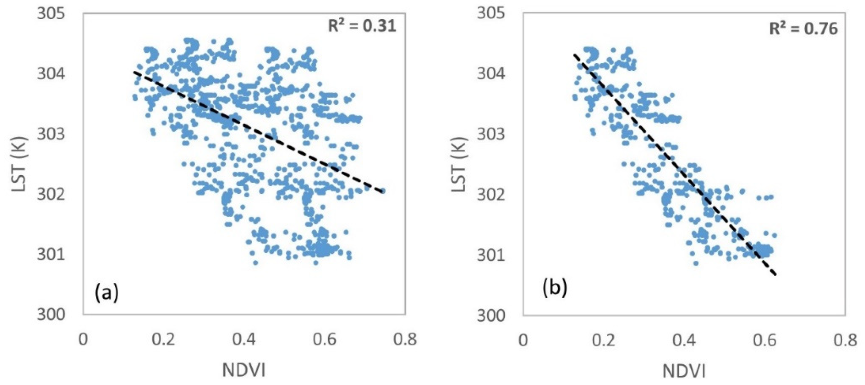
| 228–242 | 0.31 | 0.67 | 0.76 |
| 243–257 | 0.33 | 0.69 | 0.72 |
| 258–271 | 0.38 | 0.70 | 0.72 |
| 272–285 | 0.35 | 0.71 | 0.75 |
| 286–299 | 0.30 | 0.69 | 0.73 |
| 300–315 | 0.32 | 0.64 | 0.72 |
| DOY | Observed ET (mm/day) | METRIC ET (mm/day) | Fused ET (mm/day) | ||
|---|---|---|---|---|---|
| Cultivated Area | Sparse Vegetation | Cultivated Area | Sparse Vegetation | ||
| 189 | 3.5 | 3.2 | 1.1 | 2.75 | 0.4 |
| 285 | 7.2 | 6.8 | 3.5 | 6.2 | 2.4 |
| 301 | 4.3 | 4.1 | 1.8 | 4.0 | 1.6 |
| 325 | 2.9 | 2.5 | 1.0 | 2.3 | 0.3 |
| Landsat Images | No MODIS | 48-day | 40-day | 32-day | 24-day | 16-day | Hybrid | 8-day |
|---|---|---|---|---|---|---|---|---|
| 1 DOY = 189 | --- | (a) ** 2.53 53.5 4.21 | (b) ** 3.29 39.5 3.11 | (c) ** 3.47 36.3 2.86 | (d) ** 3.6 33.8 2.66 | (e) ** 4.03 25.9 2.04 | (f) ** 4.2 22.8 1.5 | (g) ** 4.26 21.7 1.4 |
| 2 DOY = 189,325 | --- | (h) ** 3.06 43.7 3.44 | (i) ** 3.51 35.4 2.79 | (j) ** 3.95 27.3 2.15 | (k) ** 4.28 21.4 1.68 | (l) ** 4.63 14.9 1.17 | (m) ** 4.73 13.0 1.1 | (n) ** 4.77 12.3 0.97 |
| 3 DOY = 189,285 325 | (o) ** 2.83 48.0 3.78 | --- | --- | (p) ** 4.30 21.0 1.65 | (q) * 4.73 13.1 1.03 | (r) ns 4.95 7.1 0.69 | (s) ns 5.00 6.5 0.61 | (t) ns 5.1 6.2 0.55 |
| 4 DOY = 189,285 301,325 | (u) ** 3.75 31.0 2.44 | --- | --- | (v) * 4.49 17.5 1.38 | (w) * 4.94 9.1 0.72 | (x) ns 5.02 6.0 0.53 | (y) ns 5.19 4.2 0.41 | (z) 5.25 3.5 0.37 |
© 2019 by the authors. Licensee MDPI, Basel, Switzerland. This article is an open access article distributed under the terms and conditions of the Creative Commons Attribution (CC BY) license (http://creativecommons.org/licenses/by/4.0/).
Share and Cite
Jamshidi, S.; Zand-Parsa, S.; Naghdyzadegan Jahromi, M.; Niyogi, D. Application of A Simple Landsat-MODIS Fusion Model to Estimate Evapotranspiration over A Heterogeneous Sparse Vegetation Region. Remote Sens. 2019, 11, 741. https://0-doi-org.brum.beds.ac.uk/10.3390/rs11070741
Jamshidi S, Zand-Parsa S, Naghdyzadegan Jahromi M, Niyogi D. Application of A Simple Landsat-MODIS Fusion Model to Estimate Evapotranspiration over A Heterogeneous Sparse Vegetation Region. Remote Sensing. 2019; 11(7):741. https://0-doi-org.brum.beds.ac.uk/10.3390/rs11070741
Chicago/Turabian StyleJamshidi, Sajad, Shahrokh Zand-Parsa, Mojtaba Naghdyzadegan Jahromi, and Dev Niyogi. 2019. "Application of A Simple Landsat-MODIS Fusion Model to Estimate Evapotranspiration over A Heterogeneous Sparse Vegetation Region" Remote Sensing 11, no. 7: 741. https://0-doi-org.brum.beds.ac.uk/10.3390/rs11070741