Sentinel-1 SAR Amplitude Imagery for Rapid Landslide Detection
by
 , , and
Alessandro C. Mondini
1,* ,
,
Michele Santangelo
1,
Margherita Rocchetti
1,
Enrica Rossetto
2,
Andrea Manconi
3 and
and
Oriol Monserrat
4 1
CNR IRPI, Via della Madonna Alta, 126, 06128 Perugia, Italy
2
Independent Researcher
3
ETH Zurich, Department of Earth Sciences, Sonneggstrasse 5, 8092 Zurich, Switzerland
4
Centre Tecnològic de Telecomunicacions de Catalunya (CTTC), Division of Geomatics, Av. Gauss 7, E-08860 Castelldefels, Barcelona, Spain
*
Author to whom correspondence should be addressed.
Remote Sens. 2019, 11(7), 760; https://0-doi-org.brum.beds.ac.uk/10.3390/rs11070760
Submission received: 12 February 2019
/
Revised: 18 March 2019
/
Accepted: 26 March 2019
/
Published: 29 March 2019
(This article belongs to the Special Issue Landslide Hazard and Risk Assessment)
Abstract
:Despite landslides impact the society worldwide every day, landslide information is inhomogeneous and lacking. When landslides occur in remote areas or where the availability of optical images is rare due to cloud persistence, they might remain unknown, or unnoticed for long time, preventing studies and hampering civil protection operations. The unprecedented availability of SAR C-band images provided by the Sentinel-1 constellation offers the opportunity to propose new solutions to detect landslides events. In this work, we perform a systematic assessment of Sentinel-1 SAR C-band images acquired before and after known events. We present the results of a pilot study on 32 worldwide cases of rapid landslides entailing different types, sizes, slope expositions, as well as pre-existing land cover, triggering factors and climatic regimes. Results show that in about eighty-four percent of the cases, changes caused by landslides on SAR amplitudes are unambiguous, whereas only in about thirteen percent of the cases there is no evidence. On the other hand, the signal does not allow for a systematic use to produce inventories because only in 8 cases, a delineation of the landslide borders (i.e., mapping) can be manually attempted. In a few cases, cascade multi-hazard (e.g., floods caused by landslides) and evidences of extreme triggering factors (e.g., strong earthquakes or very rapid snow melting) were detected. The method promises to increase the availability of information on landslides at different spatial and temporal scales with benefits for event magnitude assessment during weather-related emergencies, model tuning, and landslide forecast model validation, in particular when accurate mapping is not required.
1. Introduction
A landslide is defined as the movement of a mass of rock, debris, or earth down a slope under the influence of gravity [1]. Landslides are triggered by natural phenomena including earthquakes, rapid snow melting and intense or prolonged rainfall, or they are induced by human activities such as timber clearcut or road construction, or a combination of both [2]. They can occur singularly or in groups of tens, hundreds or even thousands in a region (We here refer to event landslide as to those slope failures appearing ‘fresh’ in remote sensing images and in the field, we also name them triggered landslides. Furthermore, we refer to a landslide event to indicate situations where multiple landslides were caused by a single triggering factor (i.e., an earthquake or a typhoon). They can also be named triggered events. An event inventory portrays a landslide event).
Landslides occur anywhere in the world causing victims, economic losses and damages to properties. Despite many authors recognize the importance of collecting accurate information on the location, type and magnitude of triggered event landslides, landslide information is lacking [3]. In many cases, landslide events can remain completely unnoticed or be only partially documented, depending on their impact on vulnerable elements (people, structures and infrastructures). This implies that knowledge on landslide triggered events can be at least biased by incomplete inventories, and reveals that our comprehension of landslides phenomena at the global/continental scale in relationship to triggering events is based on few complete event inventories [4,5]. Arguably, limited or incomplete event landslide data affects landslide modeling as well as landslide forecast models performance validation [6]. Obtaining information on landslides both in urbanized and uninhabited areas can be carried out by systematically analysing monoscopic or (better) stereoscopic aerial images available for a territory [7,8]. Generally, expert trained geomorphologists collect data on landslide occurrence by visual interpretation of such images based on a set of well-defined criteria that build on image characteristics such as color, tone, mottling, texture, object pattern (i.e., the radiometric signature), shape, size, site topography, curvature, morphologic and structural setting (i.e., the morphologic signature) [9]. If landslides are identified and mapped using archival aerial photographs, event landslide are assigned the date of the aerial photograph based on the characteristics of ‘freshness’ of slope failures, unless the date of the triggering event(s) is known. In such cases, uncertainty is introduced in assigning a date and extent to the actual triggered event. Uncertainty can be reduced drastically if landslides are detected and mapped using images acquired on-purpose right after a triggering event.
Over the last 10 years, availability of optical satellite images has significantly increased, enlarging to the global scale the potential coverage of landslide event inventory maps, also thanks to an higher revisiting time compared to aerial photographs. Optical images can be used to produce event inventories applying (i) visual interpretation or (ii) (semi-) automatic procedures. In the first case, image interpretation (along with field checks) is usually applied “on demand” because it is time consuming and expensive, hence an unknown number of landslides within triggered events can remain unnoticed or unreported. In the optical field, visual (heuristic) interpretation of images and derived products has been preparatory for (i) quantitative image analysis through image classification methods, (ii) many machine learning frameworks [10] for (iii) automatic and semi automatic recognition and mapping. The large availability of high resolution satellite data and the development of quantitative image processing techniques for event landslide detection and mapping is a potential source to systematically obtain information on slope instabilities over large areas [3,11], but it is not fully exploited, mainly because these techniques are still implemented and tested over specific test sites following already known events [12]. The systematic and/or automatic detection of new event landslides is rare [12].
Despite their undoubted potential, optical images have intrinsic limitations due to the cloud cover that usually is dense during and right after events triggered by intense rainfall [12,13]. Equatorial South America, the Congo River basin in Africa, and Southeast Asia are the cloudiest regions of the world, with annual cloud frequencies (proportion of days with a positive cloud flag) higher than eighty percent [14]. Thirtysix percent of a year of conterminous (from 30 April 2013 to 29 April 2014) United States Landsat-8 observations were obscured by cloud and an additional seven percent were obscured by cirrus. Globally, locations with very persistent cloud at the time of Landsat-5, Landsat-7, and MODIS overpass, have been observed to include Equatorial Africa, Amazonia, northern boreal regions, and Southeast Asia [15,16,17]. Darjeeling Himalayas in West Bengal province, India, witnesses every year loss of human lives and colossal damages to properties due to landslides [18]. Landslides mainly occur during the monsoon season when from June to September it rains almost every day (20/27 days each month) [18,19]. From June 2018 to September 2018, only 2 optical images in the monitoring service offered by ©2019 Planet Labs Inc. (www.planet.com) that is able to image anywhere on Earth daily with occasionally some missing date, show less than thirty percent of clouds over 58 images.
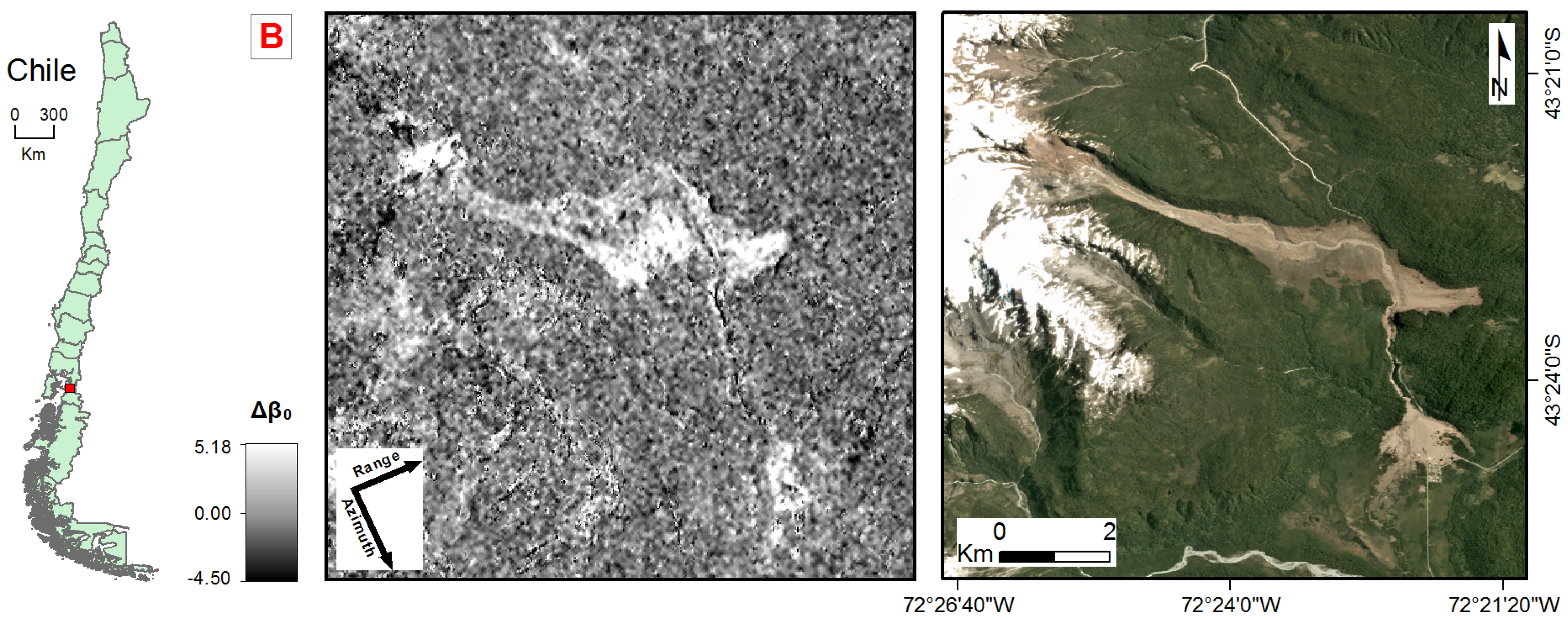
In Chile, the first cloudless image available in the service after a landslide occurred in Santa Lucia the 16 December 2017 is on the 10th of January (25 days later with 12 available images). Direct consequences can be like in the 2015 Nepal and 2016 Ecuador earthquakes crises where the unavailability of optical images hampered the capacity of the emergency response coordinators to properly cope with the event [20,21]. The use of Synthetic Aperture Radar (SAR) amplitude images can mitigate the cloud coverage issue, since the SAR signal is capable of imaging the ground surface day and night and in all weather conditions. SAR amplitude is already used to monitor land surface cover [22,23], crops [24,25], snow extent and conditions [26,27,28], glacial melt [29] and movements [30], soil moisture [31,32], and vegetation water content [33,34,35,36], to detect floods [37], natural fires [38], and earthquakes [39]. SAR products are also started to be used in rapid response situations [40], including flood services [41], to track eruption progressions [42], to produce reliable damage proxy maps of building [43] and many examples of earthquakes ground deformations maps.
All of these applications are based on measures of changes in land surface radar backscatter which can be measured by SAR-specific change detection techniques using repeat-pass imagery [36]. Most of the recently proposed SAR-based change detection techniques utilize the concept of difference images or ratio for suppressing background information and enhancing change information [44]. In a difference image, the values of the pixels associated with land cover changes present values significantly different from those of the pixels associated with unchanged areas [45,46]. Ratio image formation is helpful in suppressing image background structure and improve the detectability of potential changes from SAR data [44]. Ratio images in change detection logarithmic scaling changes the multiplicative speckle noise in the ratio-image into additive noise [47] helpful in the successive uses (classifications).
Detection of landslides by using measures of changes between pre-post amplitude SAR images is based on the assumption that landslide occurrence changes the local land cover and some of its properties (e.g., roughness and/or the complex dielectric value of the backscattering material which, in turn, depends on the moisture content [48]). When the volumetric moisture content of the top layer of the soil stripped by a landslide is high at the moment of the post event image acquisition, the backscatter signal should drop leaving dark pixels in the measures of changes. Vice-versa, new dry outcrops should result in a positive growth of the signal and then in bright pixels. Back-scattering might also increase when the roughness (at the scale of the used wavelength) increases [48]. Such modifications do not necessarily occur with all types of slope failures, but they are most commonly associated with high-mobility (i.e., rapid moving) landslides. We refer to rapid landslides as those failures that occur through a single parossistic acceleration (i.e., debris slides, avalanches, flows, and rapid deep slides) [49]. These failures present an almost complete emptying of the source area, a transit area affected in part by deposition and in part by erosion of the most superficial soil strata, whereas the accumulation zone consists mainly of completely disrupted material covering the pre-existing land surface. Landslides showing these features are often classified as rock slides, rock avalanches, debris flows, earth flows, mud flows, and lahar. For such failures, measures of the backscattered waves amplitudes recorded by some pre- and post-event SAR images may change along with the land cover, which is the basic condition for their detection [12,13,50,51].
Currently, the use of SAR amplitude images for landslide recognition and mapping is not widespread. Obstacles in their use are represented by a complex pre-processing [12,13], the acquisition geometry that can affect the quality of the images over mountainous areas where landslides are likely to occur, a certain difficulty to use the SAR signal in a traditional statistical classification approach mainly due to speckling [48], and poor familiarity to use this kind of product in the landslide mapping community. Sporadic examples exist from the use of airborne and satellite SAR data to detect, characterize, and map single landslides or single landslide events using amplitude. In a pioneering study, Singhroy et al. (1998) used Radarsat-1 images and C-HH airborne SAR data, combined with Landsat TM images, to identify diagnostic features of large landslides together with flow slides on sensitive marine clays in Canada [52]. Czuchlewski et al. (2003) employed L-band airborne SAR polarimetry to detect surface changes produced by the Tsaoling landslide, the largest slope failure triggered by the 21 September 1999 Chi-Chi 7.6 Mw earthquake in Taiwan [53]. Zhao et al. (2013) inferred the Jiweishan rock slide in China using changes in SAR backscattering intensity in ALOS/PALSAR images. Manconi et al. (2014) and Raspini et al. (2015) used very high resolution X-band COSMO-SkyMed amplitude images and pixel-offset technique for a rapid mapping of the Montescaglioso (Italy) landslide displacements [51,54]. Plank et al. (2016) combined multi-temporal information extract from optical and polarimetric SAR data to map a rotational slide near Charleston, West Virginia, USA and a mining waste earth flow near Bolshaya Talda, Russia [13]. Mondini (2017) used continuous measures of SAR amplitude changes and spatial autocorrelation to intercept hundreds of landslides occurred in Myammar in 2015 [12]. Tessari et al. (2017) measured the variation in the SAR amplitude between COSMO-SkyMed SAR acquisitions to detect the area affected by two landslides located in the North-Eastern Italian pre-Alps [55] while Konishi and Suga (2018) investigated the potential of the backscattering coefficient difference and the intensity correlation between pre- and post-disaster COSMO-SkyMed images for landslide detection in the Kii Peninsula [56].
Phase difference in SAR images and Interferometric Synthetic Aperture Radar (DInSAR) techniques have been used to identify single landslides [57,58,59,60,61] or single events [62] trough their ground displacements. Coherence between two SAR images in combination with interferometry is proposed for earthquake induced landslide detection over a large area in Nepal [40] while DInSAR and Advanced-DInSAR time-series have become common practice for deep seated slow moving landslide activity evaluation [63,64,65,66,67], landslide inventories improvements [68,69], precursor detection [70,71], and documented by the numbers of already published state of art articles [3,61,72,73,74,75,76].
The Sentinel-1 mission is enhancing the perspective in the use of SAR for landslide event disasters capturing [12]. The constellation has been specifically designed to use the phase of the SAR signal and perform, over land, advanced Differential Interferometric Synthetic Aperture Radar (DInSAR) [77].
The high revisit time, the relative high spatial resolution, the global coverage, the free availability, and new processing software, offer an unprecedented opportunity to exploit the amplitude of the SAR signal in new application fields for large scale natural hazard induced land surface changes phenomena [12,78,79]. In this work, we investigate the possibility to systematically capture rapid landslides through visual image interpretation of standard measures of amplitude changes in SAR Sentinel-1 Topsar IW-SLC images. We selected 32 worldwide events in random geo-environmental settings, land covers, type, size, and exposition. All the events occurred between May 2015 and September 2018, the period covered by the availability of Sentinel-1 images. We obtained information about landslides and their occurrence mainly using ‘the landslide blog’ (https://blogs.agu.org/landslideblog/) [80] but also searching in local newspapers, and local websites.
The procedure to pre-process the SAR images was instead the same for all test cases and included radiometric, and geometric corrections of the amplitude to obtain Beta Nought radar brightness coefficient in slant coordinates, and measures of changes of between images acquired before and after the landslide occurrence using the natural logarithm of the ratio of post event and pre event (Log-Ratio).
Maps of changes have been interpreted to detect the presence of landslides reported in the archival information selected. The test cases were classified in three main categories: landslides were (i) clearly visible; (ii) hardly visible (probably not detected if no archival information was available); (iii) not visible. The 32 test cases were then characterized based on the size of the landslides, the geometry of acquisition with respect to the slope exposition, lithology, land use, triggering factors, and climate regime.
The paper is organized as follows: in Section 2, the test cases are shortly listed and presented; Section 3 explains the work-flow to prepare the measures of changes of and the criteria adopted for the interpretation of the images; in Section 4 and Section 5, results are presented, analysed and discussed to highlight the potential of the presented technique and its limitations; in Section 6 conclusions are drawn and the future developments based on the outcomes of this work are also presented.
2. Test Cases
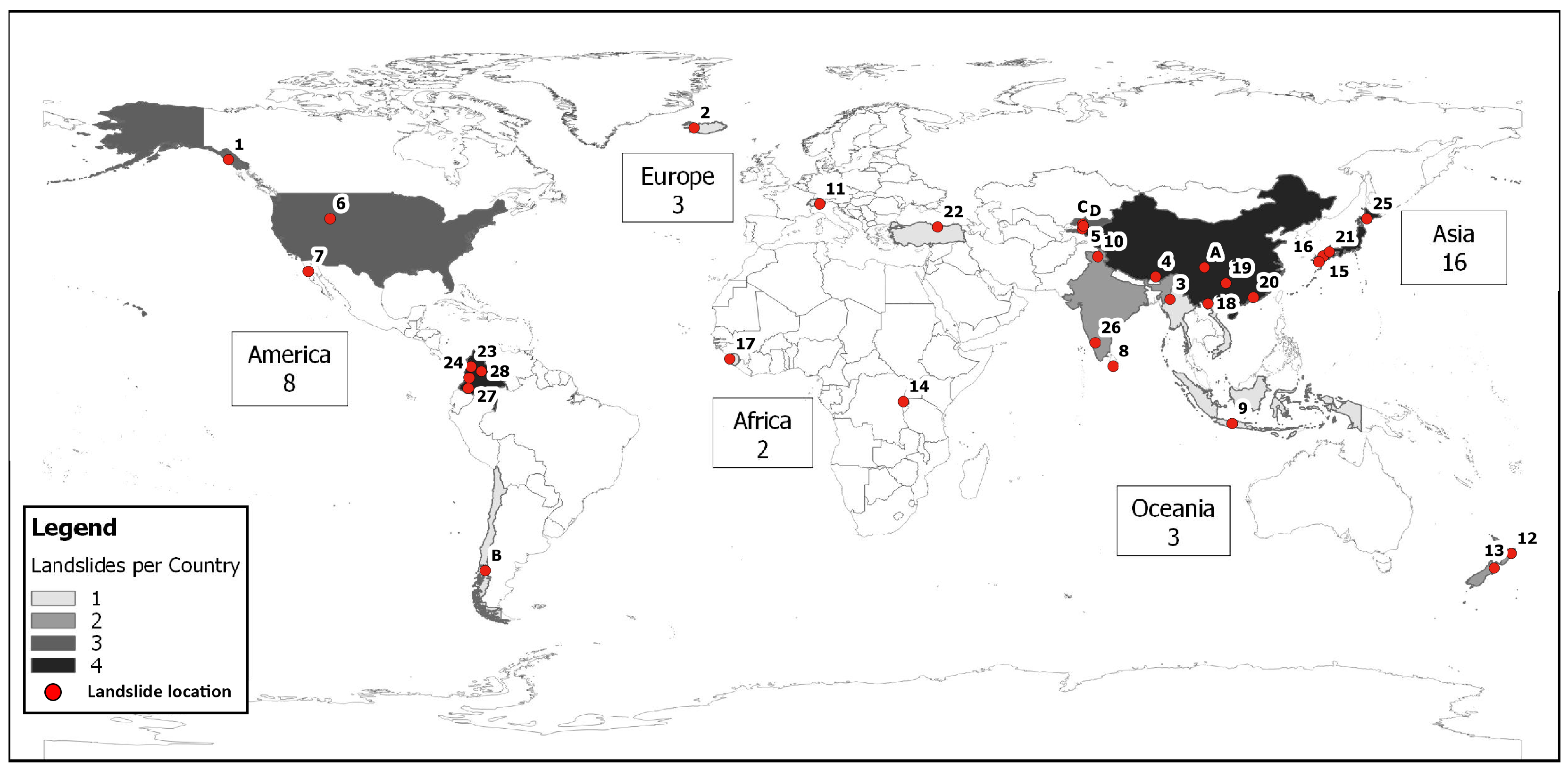
We assembled a list of 32 landslides events (Table 1) to study from a variety of different sources including reports of meteorological and seismic events that triggered slope failures, local and national newspapers available on the Internet. The main source of information was represented by the blog ‘The landslide blog’ [80,81]. The blog is continuously updated with landslide events occurring worldwide and in most of the cases together with information concerning geological aspects. The list includes two events that occurred during the writing of the paper, the first occurred during extreme monsoon rainfalls in India in August 2018 and the second, triggered by the Hokkaido Eastern Iburi Earthquake that hit the Japanese isle of Hokkaido in September 2018. fiftythree percent of selected landslides took place in Asia, about twenty five percent in America. Figure A1 in Appendix A summarizes the geographical distribution of the events. All landslides occurred in the period ranging from May 2015 to September 2018, in the temporal window nominally covered by the availability of the Sentinel-1 images. In this study we considered only rapid shallow landslides including shallow debris slides, debris avalanches, and debris flows and deep landslides including large debris slides and rock avalanches, debris flows, rock slides, and rapid earth flows [49] because they leave clear signs on the land surface. Other parameters including dimension (from 1000 m to 21 km), exposition, land cover, slope, lithology, and climate regimes were set free (Table 2). More than fifty-nine percent of the landslides are rainfall induced, and rainfall contributed together with earthquakes or rapid snow melting for twenty-one percent of the events. The triggering factors remain unknown for four cases. Lithological information was derived from different sources of information, mainly from national scale geological maps, and land cover from Google Earth. Table 1 and Table 2 resume all the information that we were able to collect for the selected cases.
3. Data and Pre-Processing
We downloaded Sentinel-1 Images from the Copernicus Open Access Hub [82] in Level-1 Single Look Complex (SLC) mode, with VV or VV-VH polarizations depending on the availability over the different test sites, and Interferometric Wide (IW) acquisition mode. SLC products are based on focused SAR data, geo-referenced using orbit and attitude data from the satellite, and provided in slant-range geometry [83]. Topsar Interferometric Wide (IW) swat mode is the main acquisition mode provided by ESA. It consists of one image per sub-swath per polarization and each sub-swath is made up of bursts as if they were independent SLC images. Size of the files ranges from 2 Gigabytes to 4 Gigabytes for single pol images in zip format, and from 4 Gigabytes to 8 Gigabytes for dual pol images respectively. As a general rule, we chose pre- and post-event images so as to have the shortest possible temporal window containing the event and, when available, in ascending and descending mode. In 17 cases the acquisition temporal window between pre- and post-event images is of 12 days, in 8 cases of 24 days, the remaining cases range between 32 and 72 days. Turkey-Giresun (Table 1, case 22, 288 days), Japan-Kumamoto (Table 1, case 16, 105 days), test cases represent an exception to this rule originated by some special event conditions described later. In two cases, the post-event image is acquired just one day after the landslide occurrence, in one case two days after. On average, only considering cases where the date of the landslide occurrence is known (27), the time delay of the used post-event acquisition is less than 10 days. Table A1 in Appendix B recaps the images used in this work.
3.1. Measures of Changes of between Pre- and Post-Event Images
The final procedure to obtain the measure of changes of amplitude between two consecutive Sentinel-1 images acquired over the same area includes: thermal noise removal, radar brightness coefficient computation in slant range or calibration [84], when available, orbit state vectors refinement with precise orbit files automatically downloaded from Array’s servers [85], Topsar de-burst, and eventually multi-looking with a number of range looks of 4 and azimuth looks of 1 to obtain a mean ground resolution square pixel of about 14 m. The two outputs are then co-registered and stacked using or (i) the SRTM 1Sec HGT auto downloaded DEM DEM-assisted co-registration, and nearest neighborhood interpolation type for the slave image (always the post-event), or (ii) the cross-correlation based co-registration with an estimate of the initial coarse offset with a width and height windows of 128, row and column interpolation factors of 4 max number of interpolations of 10 and 2000 Ground Control Points (GCPs) with a GCP tolerance of 0.25. The first represented our preferred (or first try) option, however, in some cases the procedure failed likely due to DEM inaccuracies in areas with large topographic gradients (e.g., near the Himalayan belt). Stacked images are filtered using the adaptive Frost algorithm [86], with a filter size in X and Y of 5 pixels, and a damping factor of 2. The natural logarithm of the ratio between the post-event and pre-event elaborated image is computed, and eventually ellipsoid corrected or terrain corrected to transform the measure of Intensity changes expressed by the logarithm in ground coordinates from slant coordinates. Changes can be thus visualized and interpreted in both coordinate systems.
Separately, masks of shadows and pixels in layovering were prepared to exclude from the interpretation areas with signal problems. All the pre-processing operations were assembled and executed in batch using the Graph Processing Tool (GPT) in SNAP 6.0, the software made available by ESA under the Scientific Exploitation of Operational Mission (SEOM) programme [87] Toolbox Exploitation Platform [88] for image processing.
3.2. Interpretation
We adopted a photo-interpretation approach to identify landslides in the images showing the measures of changes of . The photo interpretation approach applied to event landslide detection and mapping is usually based on the recognition of a morphological and a radiometric signature [3,9,89].
The morphological signature is the group of all the morphometric features that characterize a given slope, including slope, aspect, cross-sectional and longitudinal curvature (which allows to identify concave-convex profile slopes), roughness, among others. The morphological signature is traditionally examined using stereoscopic aerial or satellite images [3,9,89,90,91], or alternatively using high to ultra-resolution topographic data obtained by LiDAR [92,93,94] or derived through photogrammetric techniques [95] not possible in this context.
In optical images, the radiometric signature of a landslide is composed by a set of images characteristics analysed simultaneously to recognise most of the visible changes produced by an event landslide where it occurs. Such characteristics include the intensity (tone) and the wavelength (color) of the light reflected by the target, and their spatial distribution (texture, pattern, mottling, shape). Color and tone allow interpreters deriving information on the land cover (e.g., distinguishing between a bare soil and a vegetated area, or between a dry and a wet area). The spatial arrangement of the radiometric signal in the space generates what is referred to as texture, pattern, mottling and shape. In remote sensing images, such continuous features are sampled (and represented) in a grid of pixel. Therefore, the spatial arrangement of pixels is referred to the clustering of pixels showing similar tone and color characteristics. The texture refers to the granularity of the image (e.g., salt and pepper or mottled), the pattern refers to the presence of geometrical features (e.g., parallel alignments), the mottling refers to the size and distribution of the clusters of pixels within the image (e.g., darker or lighter tones areas), and the shape describes the outline of pixel clusters (e.g., elongated, irregular). Depending on the experience of the interpreters, the photo-interpretation can stop at the simple reading of the photographic and morphologic features or proceed to the identification of real-world objects, their classification and eventually make deductions about the processes.
Using images of measures of bi-temporal changes of , the detection of landslides can be done only for those landslides which have induced changes in the complex dielectric constant and or roughness of the land cover (i.e., rapid landslides). Furthermore, the dimension of the change must be enough large to visually emerge from the salt-and-pepper matrix coming from the incoherent changes occurring between two SAR images. A change of few pixels is likely to remain unnoticed in particular when the surrounding matrix of pixels shows other signatures of changes of similar sizes. From an interpreter’s point of view, in this case landslide detection can build only on considerations on the clustering of pixels with similar values of change immersed/plunged in a bulk of randomly distributed values of changes as results of changes in speckling. Therefore, the only concept that could be borrowed from the consolidated photo-interpretation technique is the analysis of the spatial distribution of the radiometric signal, which, in this case, is the pattern, texture, mottling, and shape of the clusters of pixels showing similar values of change of .
In this experiment, the assignment consisted in the ability of three differently skilled photo interpreters to detect event landslides occurred in a given space and temporal window. The process of recognition was carried out by using simultaneously images of changes in azimuth-range geometry and ellipsoidal geometry. In case of large events (many changes), subsets of 5 × 5 km around the landslides were used to constrain the search and save time.
4. Results and Analysis
Three main scenarios were identified based on the interpretation outcomes: (i) no clusters; (ii) a single clear cluster (iii) multiple clusters with different textures and shapes were identified. The first step of the interpretation consisted in detecting a cluster or a group of clusters that could correspond to the event landslide reported in the chronicle information and/or seen in the optical images. Secondly, the interpreters systematically analysed the frames to detect further clusters possibly attributable to event landslides. It was observed that single cluster scenario mainly occurred in environments without presence of snow or floods. Multiple clusters where instead detected in case of large triggered events (i.e., earthquakes or typhoons) or in presence of snow melting.
Based on these scenarios, case studies were grouped in three main categories (i) set 1: landslides were not visible; (ii) set 2: landslides were hardly visible (probably not detected if no archival information was available); (iii) set 3: landslides were clearly visible (Table 1).
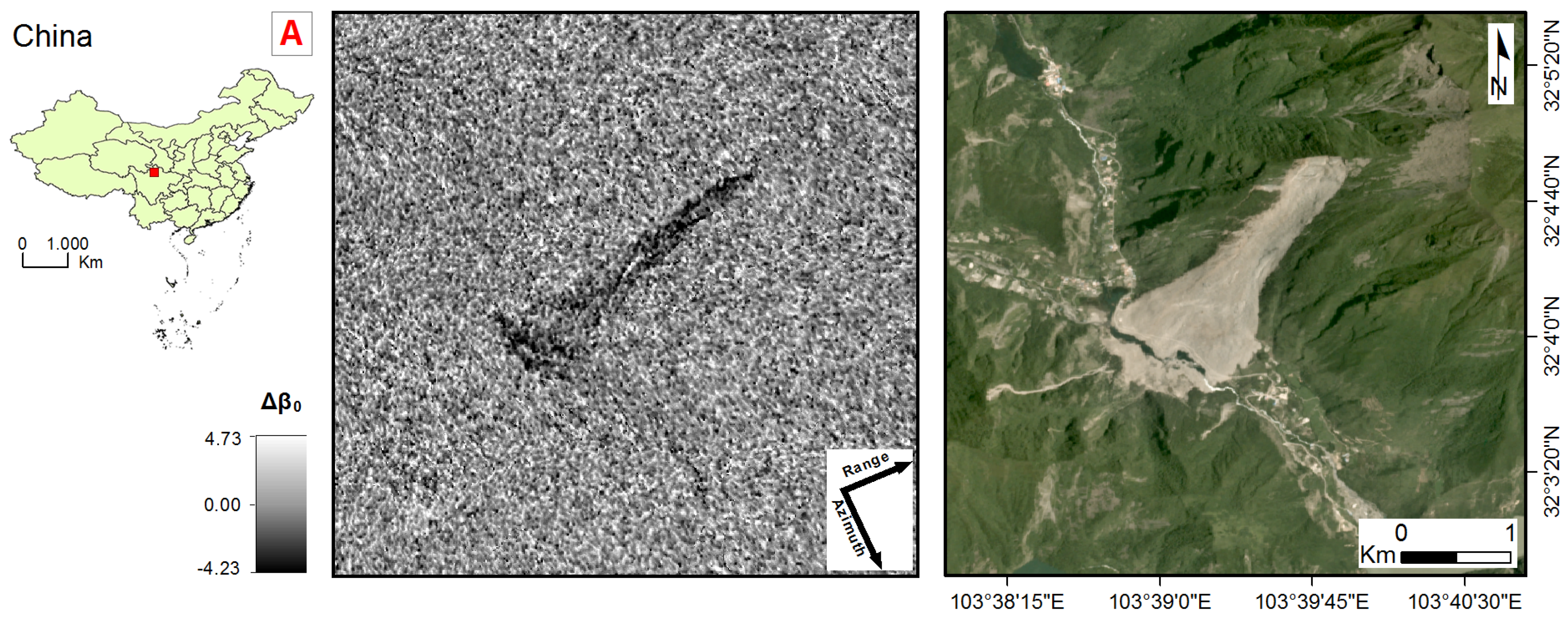
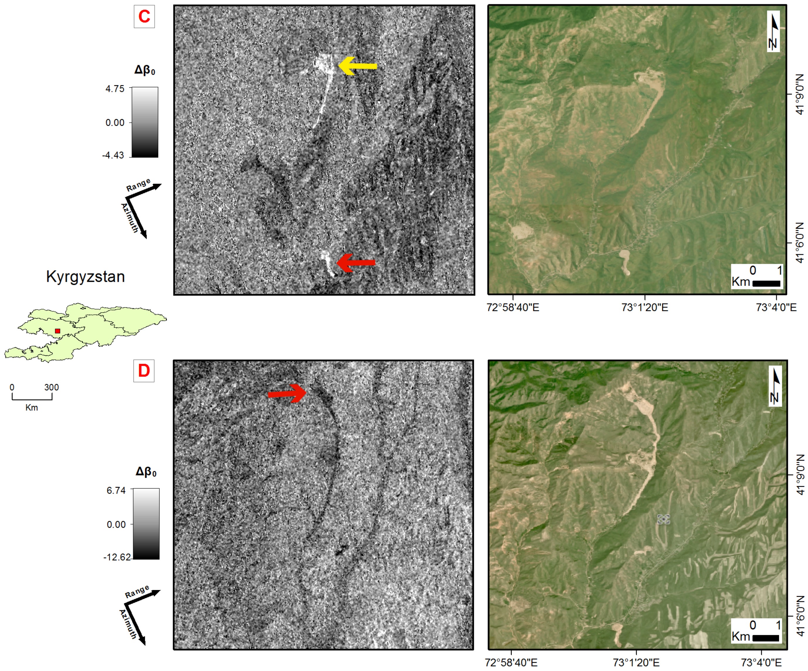
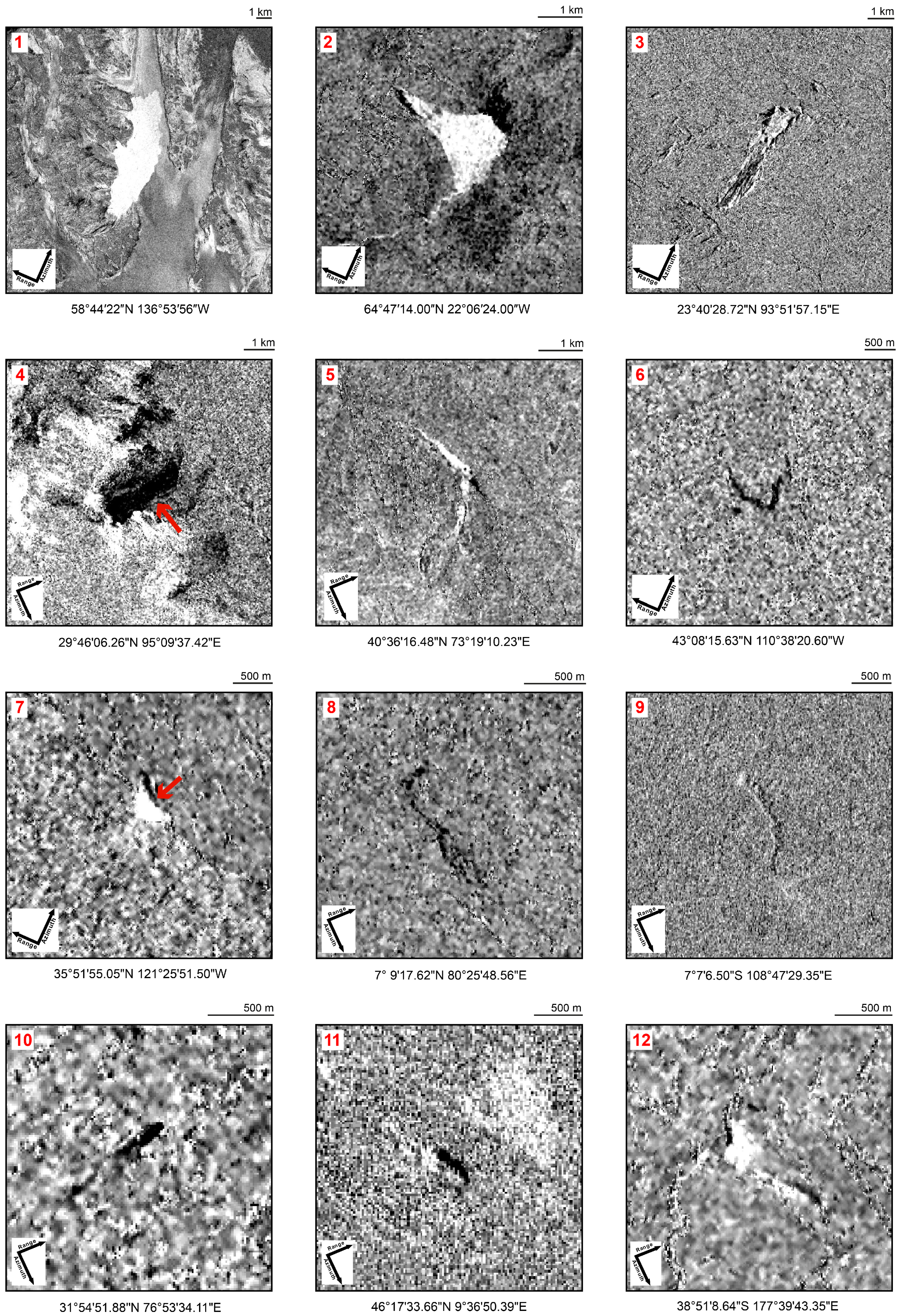
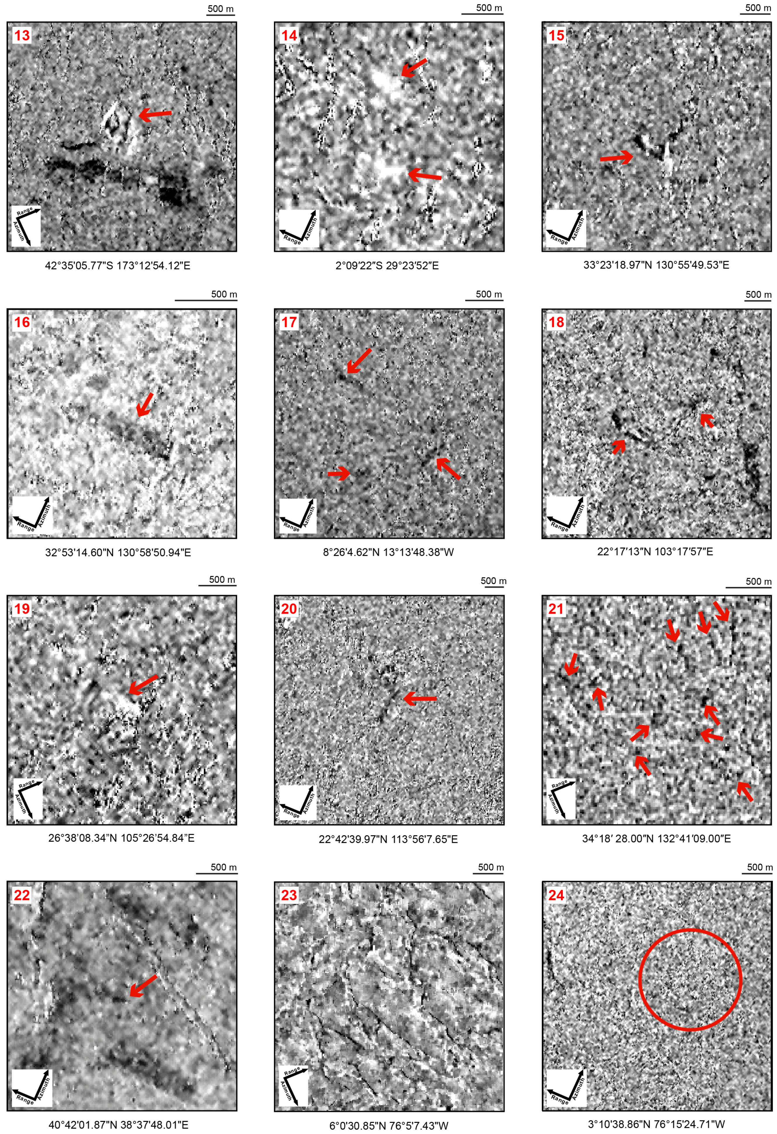
Despite the different skill of the interpreters, the agreement in the classification of the interpretation is almost total: we did not succeed in four cases (set 1), one case was identified using the coordinates (set 2), and finally we clearly identified 27 cases (set 3). In 8 cases (Table 1, cases A, B, C, D, 1, 2, 3, 4) the interpreters agreed that images show enough elements to delineate the landslide borders (mapping) and even classify their types. All results except for Colombia-Mocoa (Table 1, case 27) and Colombia-Medellin (Table 1, case 28) are shown in Figure 1, Figure 2, Figure 3, Figure 4, Figure 5 and Figure 6. Colombia-Mocoa and Colombia-Medellin landslides coordinates are approximatively 1°10′45.90″N, 76°41′4.46″W and 6°19′8.11″N, 75°29′11.39″W, respectively.
In all the figures, the measures of SAR amplitude changes are reflected over the vertical axis when satellite images are acquired in descending mode, and over the horizontal axis when satellite images are acquired in ascending mode to display landslides as closest as possible into some ground coordinates. We will now analyse the peculiarities of the test cases. General discussion on this work is demanded to the next paragraph.
Set 1 includes four test cases and they are all in Colombia. Landslides in the Colombia-Mocoa (Table 1, case 27) and Colombia-Corinto (Figure 5, case 24) test cases are multiple but very small and they occurred along narrow valleys partially North-South oriented. The first area is moderately affected by layovering (less than ten percent in the investigated area), also in proximity of the landslide, while the second is not, or just marginally. These elements might have disturbed the capacity of the interpreter to recognize the continuity of some (small) elements of changes. In particular in the Colombia-Corinto case we clearly recognized the presence of the final part of the mud flow that hit the city of Corinto, but we were not able to detect the sources (located in the red circle in Figure 5, case 24). Similarly, in the Colombia-Salgar case (Figure 5, case 23) the signs of the run-outs along the channels are visible but not the source areas.
More difficult is to justify the failure in the Colombia-Medellin (Table 1, case 28) test case having a favorable relative geometry in ascending mode. Since the landslide affected a cave, at least partially, the changes of the surface caused by the landslide might not be enough to be measured by the proposed technique.
The Turkey-Giresun test case (Figure 5, case 22) is the only one in set 2. It represents the most discussed example. The standard procedure that includes the coupling of the last pre-event image together with the first post-event image available in the ESA repository resulted too difficult to interpret. In fact, the presence of snow in the pre-event image but not in the post-event causes many signals that disturb the interpretation. Using a pre-event image without snow, the measure of changes resulted clearer but still the landslide was identified through coordinates. In particular, the geometry of the cluster was almost rectangular in shape and appeared homogeneously black in color, and then impossible to associate without unambiguity to a landslide.
Set 3 includes all the other cases, where landslides were unambiguously identified. for the SriLanka-Aranayake (Figure 4, case 8), and Japan-Kumamoto (Figure 5, case 16) cases we did not follow the standard procedure of image selection, for different reasons. In the first (SriLanka-Aranayake), we failed when we tried to co-register the first post-event to the last pre-event. We opted to use the following available post-event. The reasons for the problems in the co-registration are unknown. In the second case (Japan-Kumamoto) the images acquired close to the event have only the VV channel and in the measure of changes there are not strong signals despite of the type of situation that was supposed to be favorable. Coupling images in VH channel one acquired just after the earthquake, and one a few month later we obtained a better signal.
The effects of the acquisition mode are particularly clear in four cases. The Rwanda-Bucyurabuhoro test case (Figure 5, case 14), shows very clear signs of the target (and also of other landslides triggered in the same event) only in the ascending acquisition even if the main landslide exposition is South East. In the descending mode, there is an eastward topographic barrier in the affected slope that does not allow the signal to illuminate well the whole landslide body. The Sierra Leone-Freetown (Figure 5, case 17) test case shows well the displacement of the scarf North South oriented. Part of the end of the run out results visible as well, but it is difficult to see the connection between the two different geomorphological features, probably because the geometry is unfavorable and the lack of the descending acquisition does not help. Also the Switzerland-Bondo landslide (Figure 4, case 11), shows an extremely clear signal for most of the path to rapidly disappear because of a dramatic change in the relative geometry acquisition caused by a nearly orthogonal bend at the confluence between the channel where the landslide initiated and the valley of the main river. The Japan-Hita test case (Figure 5, case 15) is an example where the expected favorable geometry of acquisition (descending) works worse then the other (ascending) and the presence of very little layovering does not justify the result. The signal in the ascending is very clear.
The China-Shenzhen test case (Figure 5, case 20) is quite clear and there are also some evidences of the interaction between the landslide and the impacted and surrounding urban environment.
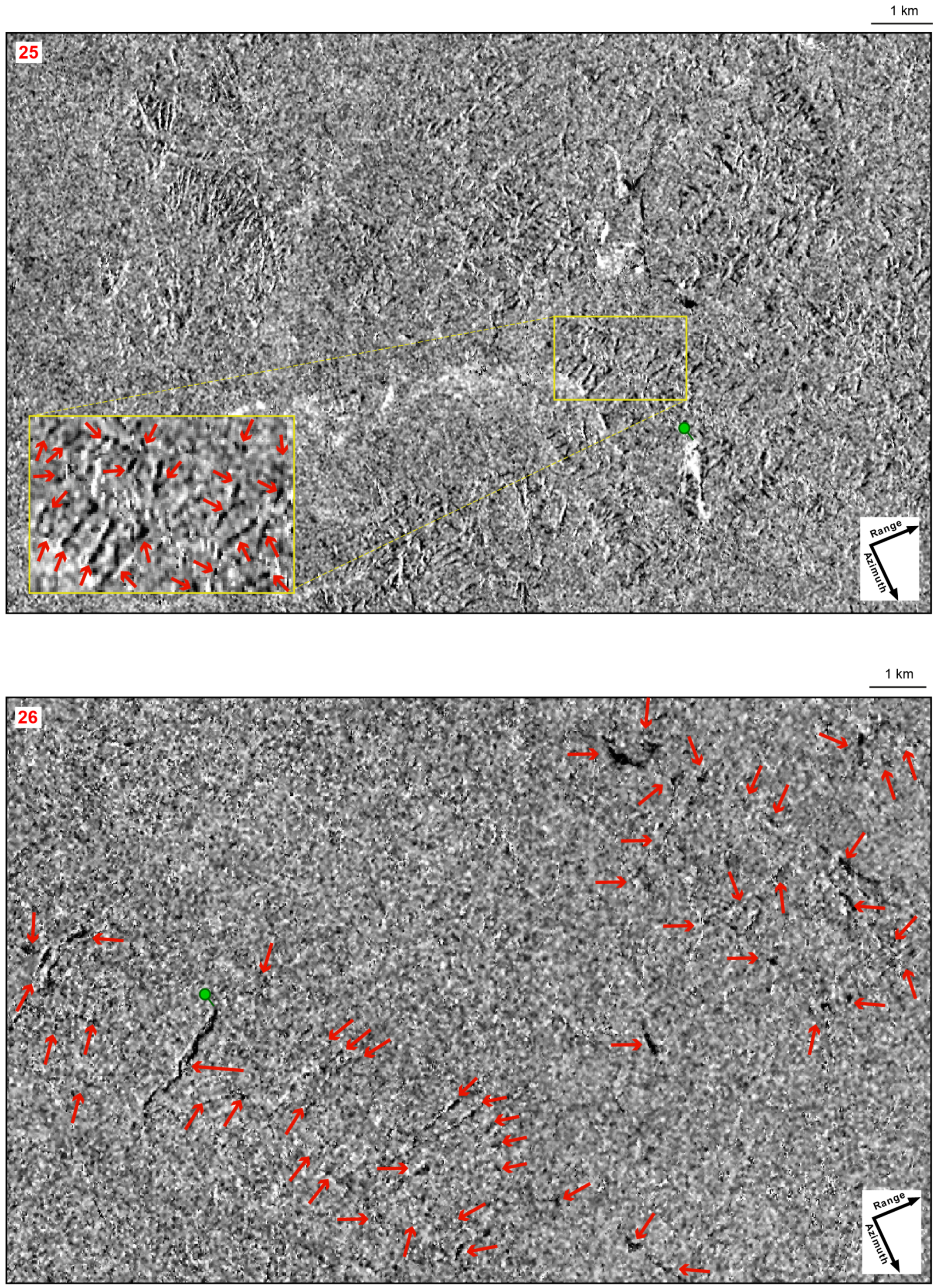
Test cases where landslides events are caused by the same triggering factors include: Myanmar-Tonzang (Figure 4, case 3), Indonesia-Pasir Panjang (Figure 4, case 9), Japan-Kure (Figure 5, case 21), and India-Kodagu (Figure 6, case 26) caused by strong rainfall, and, China-Yarlung Tsangpo (Figure 4, case 4), New Zealand-Kaikoura (Figure 5, case 13), Japan-Kumamoto (Figure 5, case 16), and Japan-Hokkaido (Figure 6, case 25) caused by earthquakes. In most of the cases, multiple signs of changes are present, including cases where landslides caused dams and then floods (New Zealand-Kaikoura, Figure 5, case 13 and, Japan-Kumamoto, Figure 5, case 16) in a multi-hazard cascade process. The landslide in Iceland (Figure 4, case 2) triggered a flood as well. Figure 6, shows spectacular examples (Japan-Hokkaido, Figure 6, case 25, and India-Kodagu, Figure 6, case 26) of event landslides intercepted by the procedure.
We did not know the date of occurrence of the China-Yarlung Tsangpo landslide (Table 1, case 4) and then we downloaded a temporal series of images that allowed us to constrain the date of occurrence in between two acquisitions (from 18 to 30 November 2017), following the big earthquake occurred the 19 November 2017. As far as we know, the precise date of occurrence remains still unknown but we can say that the landslide followed the earthquake of at least 12 days.
The remaining test cases apparently present no peculiarities and the identification resulted unambiguous and easy. In Figure 1, Figure 2 and Figure 3, respectively the China-Maoxian (case A), Chile-Villa Santa Lucia (case B), and Kyrgyzstan Amaluu-Bulak and Kyzyl-Senir (cases C and D) cases that show how landslides can be even mapped. In top left Figure 3 the yellow arrow indicates a landslide that is clearly visible in the image but it is not part of the test cases because no relative chronicle information was found. This is a landslide that might be potentially mapped.
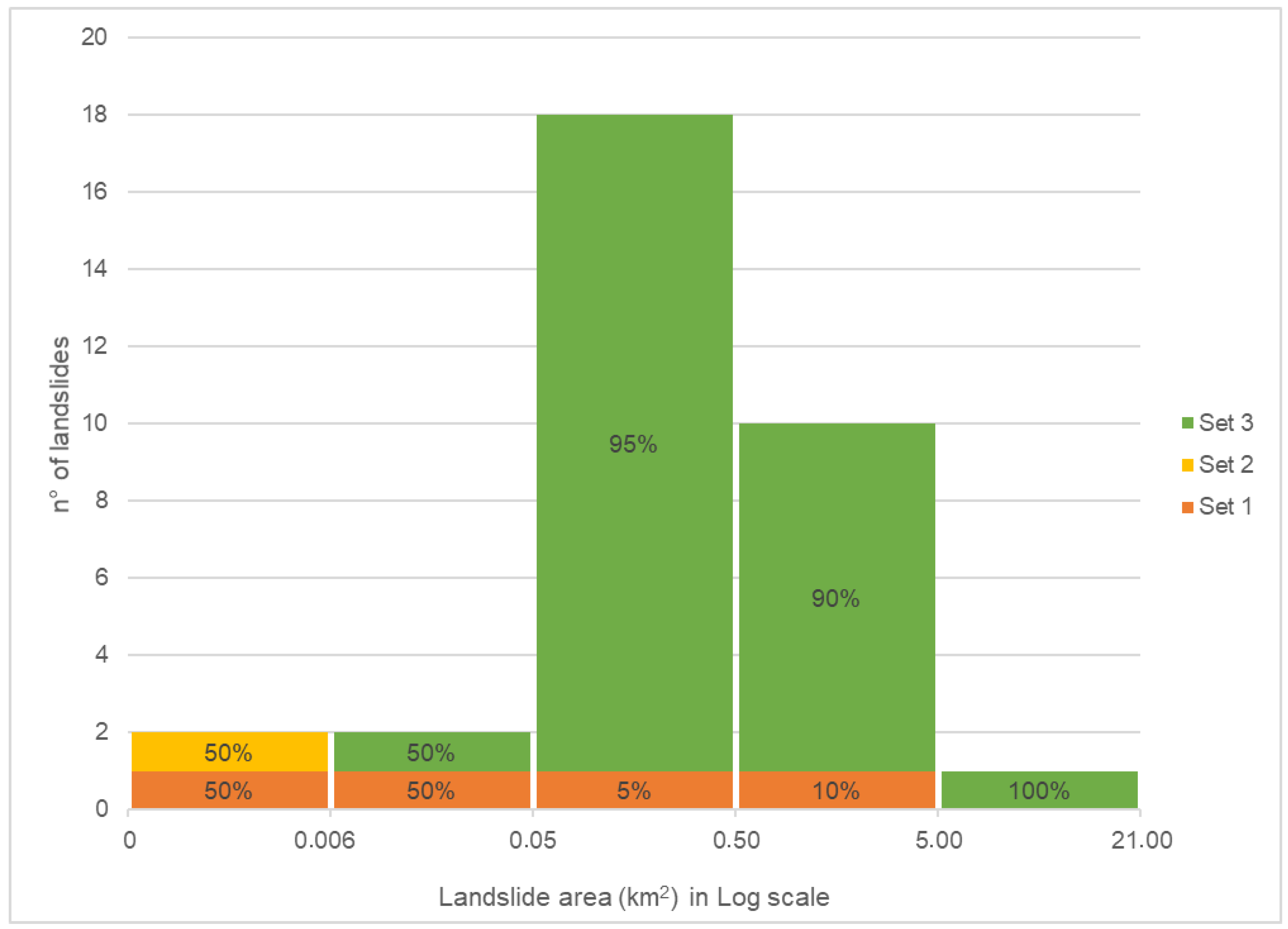
In Figure 7, the histogram displays the number of landslides in five logarithmic intervals of landslide areas. The different colors in the bars represent the different set membership percentages. The bin size was chosen to avoid empty bins.
5. Discussion
Information about landslides timely during or immediately after an event is an invaluable source for emergency response and management. We test here photo-interpretative approaches to identify rapid landslide occurrence in measures of SAR amplitude changes. The scope of the method is to obtain preliminary information when cloud coverage hampers the possibility of using optical images. We selected only cases where chronicle information reported about a high-mobility new triggered landslide occurrence, excluding a priory slow moving landslides for which many studies have been already carried out. Parameters including landslide size, direction of the movement, pre-event land cover, and triggering factors were set free in our selection.
The pre-processing of the images was the same for all the test cases with the purpose of evaluating its systematic applicability in different contexts. Occasionally, exceptions were done for the co-registration. We acknowledge that some test cases would have probably benefited of some ad-hoc tuning.
We worked with Level-1 SLC products because, in the past, more frequently available than Level-1 GRD products, they are not multi-looked, and they are in SAR coordinates allowing more options in the tuning of the pre-processing procedure. We verified that the multi-looking process, in particular with a Number of Range Looks of 4 and Azimuth Looks of 1 to obtain a ground square pixel of about 14 m, tends to produce maps more familiar to the interpreter. In fact they look more similar to the maps commonly used in terms of noise, orientation and proportions (less distorted). Figure 1, Figure 2 and Figure 3 show how the landslides features in the SAR measures of changes might still present some deformations in comparison with optical images that are caused by the use of a different reference system. Distortions required an adaptation effort in the photo-interpretation process. For very small features, the recognition of changes resulted in many cases ambiguous but easier measuring changes at higher spatial resolution before the multi-looking. The re-projection in ground coordinates introduces some tedious distortions that can affect the interpretation, particularly when landslides are small and they occur on steep slopes. In order to recognize changes caused by landslides and some geomorphological features, the final preference has been mainly assigned to maps in SAR coordinates with multi-looking.
All the downloaded images were in Interferometric Wide (IW) mode with 5 × 20 m spatial resolution in single look. IW is the main acquisition mode over land. We presume that some Strip Map mode images at 5 × 5 m spatial resolution in single look would have helped in recognizing changes in sets 1 and 2, and perhaps in a better definition of some local features of changes associated to the landslides under study. It is known that the detectability of small landslides increases with the increasing spatial resolution of optical images [9]. This has to be tested for SAR images. When available, we processed both VV, and VH channels and we noticed a better definition of the changes in the VH channel when landslides occurred in previously deeply vegetated areas, while VV offers sometimes more definition and contrast in presence of glaciers or snow. The interpretation was facilitated in presence of both the channels. We bore an unexpected problem at the level of co-registration when we analysed areas close to the Himalayan chain. The DEM-assisted co-registration procedure generated some triangular lacerations into the co-registered images in some cases involving the area affected by the changes. In these cases we co-registered the images using the procedure available in SNAP based on cross correlation. Comparative tests randomly selected (Table 1, cases 11, 15, 24, B, C) between the two procedures in areas where we did not experience problems in using the DEM-based procedure, did not show any influence of using one of the two procedures on the result.
We opted for a unique speckling filter set-up based on the Frost filter, which was already proved that suitable for working properly in mountainous areas [96] where landslides occur. The 5 × 5 moving window size represents a compromise between the need of the interpreter to (i) preserve the features potentially related to changes caused by small landslides and (ii) filter the noise. It was chosen through a trial and error process according to the preferences of the interpreters. Moving windows larger than 5 × 5 resulted too invasive and able to cover some features important for the interpretation of small landslides. The difference between 3 × 3 and 5 × 5 moving windows is not impacting and somehow difficult to evaluate.
Photo-interpretative methods cover the problems generated by the adaptive filters outliers [46,97] in the Log-Ratio index unsupervised thresholds identifications to detect changes. The Log-Ratio index is a conservative choice: it is widely used in many applications, relatively easy to implement, less sensitive to to calibration errors compared to the traditional methods based on differences [36], adapt to o enhance low-intensity pixels [35] to facilitate the interpretation in particular after multi-looking [36], and proved to be useful to detect landslides [12]. Speckling filtering is probably one of the main steps where dedicated solutions and tuned parameters would contribute more to reach, case by case, better results.
The geometry of a SAR image acquisition system, or the relative geometry between the satellite transmission/acquisition system and the target is an information to take into account in the interpretation of a SAR image. We adopted the criterion of choosing, as first try, the geometry of acquisition that should limit geometrical distortions in the single images and then in the change detection estimation, with ascending acquisitions for landslides exposed towards West, descending acquisitions for landslides exposing towards East and no preference for North-South moving direction. This criterion was not always respected due to the lack of images in both the acquisition configurations. When possible, we used both ascending and descending acquisitions for the interpretation of the same event. Our choice was betrayed at least in the Kumamoto-Japan test case (Table 1, case 16).
The relative geometry is a key point for the SAR intrinsic geometry distortions including layovering, shadowing and foreshortening that remain insurmountable limitations in the use of the images. The problem can be just partially mitigated by using the double orbit (ascending and descending) when available. This is somehow more evident for small landslides that induce limited changes difficult to trap when immersed in the salt and pepper noise originated by the random changes experienced between the pre- and post-event images.
There is a limit to landslide detection that is imposed by the images resolution, the limit is not absolute because it also depends on the signal contrast between within and outside the landslide border. The detection of event landslides in remote sensing optical images builds on the ability of an interpreter to discern the signature of the landslide from its neighboring area. Landslides are perceived by interpreters as anomalies in otherwise continuous features that characterize a landscape, such as land-use pattern (plowing, wood, cultivated land), anthropic elements (e.g., linear infrastructures), geological structures (bedding traces, faults traces), among others. The more the landslide signature (morphological and photographic in optical images) is different from the typical surrounding environment, the easier it can be detected by an image interpreter. For example, shallow landslides are harder to detect on a not plowed and not vegetated field during the autumn/winter seasons than on a grass-covered field. In our case, the only variables that can be taken into account are the pattern and shape of the clusters the portray the perturbation induced by the landslide occurrence, given that a change has occurred where clusters appear. There is no morphological elements, nor photographical elements that an interpreter can associate to a landslide feature or to an entire landslide. Our set of cases and imagery do not allow us to determine the lower limit of the detectable landslide size and more research is needed.
The other variables taken into account in this work, include geology and pre-existing land cover. All of them do not seem to influence the ability of the interpreter to recognize landslides. Landslides occurred in areas previously covered by vegetation resulted in some cases easier to detect, particularly in the VH channel. Earthquakes, rapid snow melting, and typhoons may cause situations with diffuse and different signs on the territory. In many cases, situations of cascade multi-hazard were found, particularly floods caused by landslide dams. Cases with single landslides resulted definitely much easier to detect, but the learning process experienced by the interpreters allowed to identify landslides previously unknown. This was particularly relevant for the events triggered by earthquakes in China, Japan, New Zealand, Myanmar, and in Kyrgyzstan.
We also stress that in some cases we were looking for a single landslide and we found populations of landslides caused by the same triggering factor. Examples are the Kaikoura case in New Zealand (Figure 5, case 13), the Amaluu-Bulak case in Kyrgyzstan (Figure 3, case C), the Kumamoto case in Japan (Figure 5, case 16), the Pasir Panjang case in Indonesia (Figure 4, case 9) and the Tonzang case in Myanmar (Figure 4, case 3). This can be seen as an indication that the photo-interpreter has increased the ability to associate patterns of emerging clusters of changes to landslides independently by an priori information.
The Hokkaido case in Japan and the Kodagu case in India (Figure 6, cases 25 and 26) encourage to speculate the use of the technique for a rapid identification of the areas affected by huge triggering events. Myanmar (Figure 4, case 3) and Japan (Figure 5, case 16) are other meaningful examples. For these events magnitude estimation, which requires a quantitative assessment of the number and the size of the triggered landslides, we consider worthwhile to carry out further research.
In at least two (Figure 5, cases 23 and 24) of the four unsuccessful cases we were able to identify some consequences of the event. This information can also be used for emergency purposes.
The good results obtained at least in 28 cases allow to state that the framework is enough general to be used worldwide to detect triggered high-mobility landslides. Results encourage for further research that might include fine tuning of the procedure according to the geo-environmental characteristics of specific areas, the use different measures of changes, the use of higher spatial resolution SAR images to overcome the problems of the interpreters in the recognition of small landslides or features (Figure 7), in different bands and polarizations and DEMs, in particular to increase the capacity of recognize small landslides.
6. Conclusions
This study applied photo-interpretative methods to detect landslides in measures of changes of amplitude in pre- and post-event Sentinel-1 images. The method was exploited in 32 cases worldwide. Landslides events are variegated and include single landslides or families of landslides caused by the same triggering factor, earthquakes, rapid snow melt, or intense rainfalls. They are all rapid landslides but vastly different in size, exposition, process and geographical, geological, and geomorphological settings. Photo-interpreters were able to capture 27 cases with the possibility of mapping features in at least 8 cases. One case was detected a posteriori knowing where the landslide occurred while in the remaining four cases (all in Colombia), the interpretation did not clearly recognize signs ascribable to landslides but to secondary effects like deposits at the end of the runouts. The rate of success of this study suggests that SAR Sentinel-1 images and photo-interpretation are a reliable combination for capturing rapid landslides. All weather SAR images permit to obtain information about the landslide occurrence during an rain event when optical images are not available or useless because of cloud presence with clear benefits in terms of disaster management civil protection operations. Furthermore, the unprecedented availability of Sentinel-1 images in terms of frequency of acquisition and spatial coverage promises to foster the production of information at global scale with positive feedbacks on the quality of hazard mapping and risk assessments and climate change impact evaluation. This study is vanguard (pioneer) and it shows many topics that merit future research. Priorities are given to: (i) customization of the procedure to measure changes according to specific test sites requirements, (ii) use ground coordinates, and (iii) and more in general, consolidate the learning process on the use of the SAR images.
Author Contributions
A.C.M. designed and coordinated the work, executed data processing and wrote the manuscript. M.S. photo interpreted the results and wrote the manuscript, M.R. executed data processing, photo interpreted the results, and wrote the manuscript, E.R. executed data processing and photo interpreted the results, A.M. and O.M. co-designed the work and wrote the manuscript.
Funding
This research was supported by the UKRI Natural Environment Research Council’s and UK Government’s Department for International Development’s Science for Humanitarian Emergencies and Resilience research programme (grant number NERC/DFID NE/P000649/1).
Acknowledgments
We thank the anonymous reviewers for their careful reading of our manuscript and their insightful comments and suggestions.
Conflicts of Interest
The authors declare no conflict of interest.
Appendix A
Figure A1.
Geographical distribution of the events (Table 1).
Figure A1.
Geographical distribution of the events (Table 1).

Appendix B

Table A1.
Sentinel-1 images used to retrieve the measures of amplitude changes.
| ID | Track | Orbit | POST EVENT Image | PRE EVENT Image |
|---|---|---|---|---|
| 1 | 152 | Ascending | S1A_IW_SLC__1SSV_20160806T024605_20160806T024633_012474_0137F7_D97D | S1A_IW_SLC__1SSV_20160526T024600_20160526T024628_011424_011617_44DD |
| 2 | 16 | Ascending | S1A_IW_SLC__1SDV_20180717T185857_20180717T185924_022838_0279F5_B025 | S1A_IW_SLC__1SDV_20180623T185856_20180623T185923_022488_026F84_32C6 |
| 3 | 143 | Ascending | S1A_IW_SLC__1SSV_20150811T114745_20150811T114812_007215_009DE4_76C9 | S1A_IW_SLC__1SSV_20150718T114744_20150718T114811_006865_00942A_2799 |
| 4 | 4 | Descending | S1A_IW_SLC__1SDV_20171130T233727_20171130T233754_019501_02117D_7793 | S1A_IW_SLC__1SDV_20171118T233727_20171118T233754_019326_020C05_F81A |
| 5 | 5 | Descending | S1A_IW_SLC__1SSV_20160504T011247_20160504T011314_011102_010BB5_702B | S1A_IW_SLC__1SSV_20160410T011247_20160410T011313_010752_0100E1_B6A9 |
| 6 | 122 | Ascending | S1A_IW_SLC__1SDV_20170606T011848_20170606T011915_005923_00A638_1C81 | S1B_IW_SLC__1SDV_20170525T011847_20170525T011914_005748_00A123_B3E7 |
| 7 | 35 | Ascending | S1B_IW_SLC__1SDV_20170531T020608_20170531T020635_005836_00A3AE_1AA5 | S1B_IW_SLC__1SDV_20170519T020608_20170519T020635_005661_009EA1_7930 |
| 8 | 19 | Descending | S1A_IW_SLC__1SSV_20160716T002448_20160716T002516_012166_012DD0_1B6A | S1A_IW_SLC__1SSV_20160505T002441_20160505T002509_011116_010C15_C69F |
| 9 | 149 | Descending | S1A_IW_SLC__1SDV_20180304T222520_20180304T222548_020871_023CCB_9BD6 | S1A_IW_SLC__1SDV_20180220T222520_20180220T222548_020696_023742_C994 |
| 10 | 136 | Descending | S1A_IW_SLC__1SDV_20170824T005106_20170824T005133_018058_01E522_0F86 | S1A_IW_SLC__1SDV_20170812T005105_20170812T005132_017883_01DFD4_6567 |
| 11 | 66 | Descending | S1B_IW_SLC__1SDV_20170825T053412_20170825T053439_007092_00C7F7_8018 | S1B_IW_SLC__1SDV_20170813T053411_20170813T053438_006917_00C2E7_8739 |
| 12 | 175 | Descending | S1A_IW_SLC__1SDV_20180306T172124_20180306T172154_020897_023D98_F7AC | S1A_IW_SLC__1SDV_20180222T172124_20180222T172154_020722_02380F_4AEE |
| 13 | 73 | Descending | S1A_IW_SLC__1SSV_20161116T173100_20161116T173127_013970_016811_1786 | S1A_IW_SLC__1SSV_20160905T173100_20160905T173127_012920_0146D2_B6AC |
| 14 | 174 | Ascending | S1A_IW_SLC__1SDV_20180517T162025_20180517T162025_021946_025EAC_6C74 | S1A_IW_SLC__1SDV_20180505T162024_20180505T162051_021771_02591D_2CC1 |
| 15 | 156 | Ascending | S1B_IW_SLC__1SDV_20170714T091327_20170714T091402_006482_00B65B_40D7 | S1B_IW_SLC__1SDV_20170702T091326_20170702T091401_006307_00B16E_AE76 |
| 16 | 54 | Ascending | S1A_IW_SLC__1SDV_20160519T092157_20160519T092224_011326_0112E1_78CD | S1A_IW_SLC__1SDV_20151203T092153_20151203T092220_008876_00CB00_AB71 |
| 17 | 60 | Ascending | S1A_IW_SLC__1SDV_20170818T190805_20170818T190832_017982_01E2CF_BCD8 | S1A_IW_SLC__1SDV_20170806T190804_20170806T190831_017807_01DD81_C220 |
| 18 | 26 | Ascending | S1A_IW_SLC__1SDV_20180718T111440_20180718T111507_022848_027A43_386E | S1A_IW_SLC__1SDV_20180612T111438_20180612T111505_022323_026A94_19D0 |
| 19 | 164 | Descending | S1A_IW_SLC__1SDV_20170906T225727_20170906T225755_018261_01EB46_0B57 | S1A_IW_SLC__1SDV_20170825T225727_20170825T225755_018086_01E5F4_9E67 |
| 20 | 11 | Ascending | S1A_IW_SLC__1SDV_20151224T103309_20151224T103339_009183_00D39A_1C3B | S1A_IW_SLC__1SDV_20151212T103310_20151212T103340_009008_00CEA9_624B |
| 21 | 90 | Descending | S1A_IW_SLC__1SDV_20180710T210818_20180710T210846_022737_0276D8_9F2E | S1A_IW_SLC__1SDV_20180628T210818_20180628T210845_022562_0271AB_CB0A |
| 22 | 43 | Ascending | S1A_IW_SLC__1SDV_20160224T151754_20160224T151821_010090_00EDDE_760B | S1A_IW_SLC__1SDV_20150512T151748_20150512T151815_005890_00795C_FD88 |
| 23 | 142 | Descending | S1A_IW_SLC__1SSV_20150531T105025_20150531T105052_006164_00804A_A3BF | S1A_IW_SLC__1SSV_20150507T105023_20150507T105050_005814_0077A0_F26B |
| 24 | 48 | Ascending | S1B_IW_SLC__1SDV_20171115T232058_20171115T232125_008299_00EAEE_E985 | S1B_IW_SLC__1SDV_20171103T232058_20171103T232125_008124_00E5AE_F328 |
| 25 | 46 | Descending | S1A_IW_SLC__1SDV_20180905T204111_20180905T204139_023568_029131_BE2C | S1A_IW_SLC__1SDV_20180824T204111_20180824T204138_023393_028B99_998A |
| 26 | 63 | Descending | S1A_IW_SLC__1SDV_20180826T004813_20180826T004840_023410_028C24_DF28 | S1A_IW_SLC__1SDV_20180802T004811_20180802T004838_023060_0280E6_1133 |
| 27 | 142 | Descending | S1B_IW_SLC__1SSV_20170408T105103_20170408T105131_005068_008DD8_FE30 | S1B_IW_SLC__1SSV_20170327T105103_20170327T105131_004893_0088CA_547D |
| 28 | 150 | Ascending | S1B_IW_SLC__1SDV_20161103T231341_20161103T231409_002801_004BE6_7629 | S1B_IW_SLC__1SDV_20161010T231341_20161010T231409_002451_00422E_DE56 |
| A | 62 | Descending | S1A_IW_SLC__1SDV_20170713T230410_20170713T230437_017459_01D2E8_0F0C | S1A_IW_SLC__1SDV_20170619T230409_20170619T230436_017109_01C859_BEC5 |
| B | 83 | Descending | S1B_IW_SLC__1SDV_20171224T095748_20171224T095815_008859_00FC9E_99BC | S1B_IW_SLC__1SDV_20171212T095748_20171212T095815_008684_00F709_A672 |
| C | 5 | Descending | S1A_IW_SLC__1SSV_20160504T011247_20160504T011314_011102_010BB5_702B | S1A_IW_SLC__1SSV_20160410T011247_20160410T011313_010752_0100E1_B6A9 |
| D | 5 | Descending | S1A_IW_SLC__1SSV_20160504T011247_20160504T011314_011102_010BB5_702B | S1A_IW_SLC__1SSV_20160410T011247_20160410T011313_010752_0100E1_B6A9 |
References
- Cruden, D.M.; Varnes, D.J. Landslide types and processes. In Landslides, Investigation and Mitigation, Special Report 247; Turner, A., Schuster, R., Eds.; Transportation Research Board: Washington, DC, USA, 1996; pp. 36–75. [Google Scholar]
- Aleotti, P.; Chowdhury, R. Landslide hazard assessment: Summary review and new perspectives. Bull. Eng. Geol. Environ. 1999, 58, 21–44. [Google Scholar] [CrossRef]
- Guzzetti, F.; Mondini, A.C.; Cardinali, M.; Fiorucci, F.; Santangelo, M.; Chang, K.T. Landslide inventory maps: New tools for an old problem. Earth Sci. Rev. 2012, 112, 42–66. [Google Scholar] [CrossRef] [Green Version]
- Guzzetti, F.; Malamud, B.D.; Turcotte, D.L.; Reichenbach, P. Power-law correlations of landslide areas in central Italy. Earth Planet. Sci. Lett. 2002, 195, 169–183. [Google Scholar] [CrossRef]
- Malamud, B.D.; Turcotte, D.L.; Guzzetti, F.; Reichenbach, P. Landslide inventories and their statistical properties. Earth Surf. Process. Landf. 2004, 29, 687–711. [Google Scholar] [CrossRef]
- Rossi, M.; Guzzetti, F.; Reichenbach, P.; Mondini, A.C.; Peruccacci, S. Optimal landslide susceptibility zonation based on multiple forecasts. Geomorphology 2010, 114, 129–142. [Google Scholar] [CrossRef]
- Dikau, R. The recognition of landslides. In Floods and Landslides: Integrated Risk Assessment; Casale, R., Margottini, C., Eds.; Springer: Berlin/Heidelberg, Germany, 1999; pp. 39–44. [Google Scholar]
- Saba, S.B.; van der Meijde, M.; van der Werff, H. Spatiotemporal landslide detection for the 2005 Kashmir earthquake region. Geomorphology 2010, 124, 17–25. [Google Scholar] [CrossRef]
- Fiorucci, F.; Giordan, D.; Santangelo, M.; Dutto, F.; Rossi, M.; Guzzetti, F. Criteria for the optimal selection of remote sensing optical images to map event landslides. Nat. Hazards Earth Syst. Sci. 2018, 18, 405–417. [Google Scholar] [CrossRef] [Green Version]
- Kanevski, M.; Pozdnoukhov, A.; Timonin, V. Machine Learning for Spatial Environmental Data: Theory, Applications and Software; EPFL Press: Lausanne, Switzerland; Boca Raton, FL, USA, 2009; p. 377. [Google Scholar]
- Martha, T.R.; Kerle, N.; van Westen, C.J.; Jetten, V.; Kumar, K.V. Segment Optimization and Data-Driven Thresholding for Knowledge-Based Landslide Detection by Object-Based Image Analysis. IEEE Trans. Geosci. Remote Sens. 2011, 49, 4928–4943. [Google Scholar] [CrossRef]
- Mondini, A.C. Measures of Spatial Autocorrelation Changes in Multitemporal SAR Images for Event Landslides Detection. Remote Sens. 2017, 9, 554. [Google Scholar] [CrossRef]
- Plank, S.; Twele, A.; Martinis, S. Landslide Mapping in Vegetated Areas Using Change Detection Based on Optical and Polarimetric SAR Data. Remote Sens. 2016, 8, 307. [Google Scholar] [CrossRef]
- Wilson, A.M.; Jetz, W. Remotely Sensed High-Resolution Global Cloud Dynamics for Predicting Ecosystem and Biodiversity Distributions. PLoS Biol. 2016, 14, e1002415. [Google Scholar] [CrossRef]
- Li, J.; Roy, D.P. A Global Analysis of Sentinel-2A, Sentinel-2B and Landsat-8 Data Revisit Intervals and Implications for Terrestrial Monitoring. Remote Sens. 2017, 9, 902. [Google Scholar] [Green Version]
- Kovalskyy, V.; Roy, D. The global availability of Landsat 5 TM and Landsat 7 ETM+ land surface observations and implications for global 30m Landsat data product generation. Remote Sens. Environ. 2013, 130, 280–293. [Google Scholar] [CrossRef] [Green Version]
- Ju, J.; Roy, D.P. The availability of cloud-free Landsat ETM+ data over the conterminous United States and globally. Remote Sens. Environ. 2008, 112, 1196–1211. [Google Scholar] [CrossRef]
- Surendranath, M.; Ghosh, S.; Ghoshal, T.B.; Rajendran, N. Landslide Hazard Zonation in Darjeeling Himalayas: A Case Study on Integration of IRS and SRTM Data. In Remote Sensing and GIS Technologies for Monitoring and Prediction of Disasters; Nayak, S., Zlatanova, S., Eds.; Springer: Berlin/Heidelberg, Germany, 2008; pp. 121–135. [Google Scholar]
- Starkel, L. The Role of Catastrophic Rainfall in the Shaping of the Relief of the Lower Himalaya (Darjeeling Hills). Geogr. Polon. 1972, 21, 103–160. [Google Scholar]
- Williams, J.G.; Rosser, N.J.; Kincey, M.E.; Benjamin, J.; Oven, K.J.; Densmore, A.L.; Milledge, D.G.; Robinson, T.R.; Jordan, C.A.; Dijkstra, T.A. Satellite-based emergency mapping using optical imagery: Experience and reflections from the 2015 Nepal earthquakes. Nat. Hazards Earth Syst. Sci. 2018, 18, 185–205. [Google Scholar] [CrossRef]
- BGS. Ecuador Earthquake Disaster Response. 2016. Available online: https://www.bgs.ac.uk/research/earthHazards/epom/ecuadorEarthquake.html (accessed on 28 January 2019).
- Da Costa Freitas, C.; de Souza Soler, L.; Sant’Anna, S.J.S.; Dutra, L.V.; dos Santos, J.R.; Mura, J.C.; Correia, A.H. Land Use and Land Cover Mapping in the Brazilian Amazon Using Polarimetric Airborne P-Band SAR Data. IEEE Trans. Geosci. Remote Sens. 2008, 46, 2956–2970. [Google Scholar] [CrossRef]
- Lonnqvist, A.; Rauste, Y.; Molinier, M.; Hame, T. Polarimetric SAR Data in Land Cover Mapping in Boreal Zone. IEEE Trans. Geosci. Remote Sens. 2010, 48, 3652–3662. [Google Scholar] [CrossRef]
- Xu, H.; Steven, M.D.; Jaggard, K.W. Monitoring leaf area of sugar beet using ERS-1 SAR data. Int. J. Remote Sens. 1996, 17, 3401–3410. [Google Scholar] [CrossRef]
- Yang, Z.; Li, K.; Liu, L.; Shao, Y.; Brisco, B.; Li, W. Rice growth monitoring using simulated compact polarimetric C band SAR. Radio Sci. 2014, 49, 1300–1315. [Google Scholar] [CrossRef] [Green Version]
- Guneriussen, T.; Johnsen, H.; Sand, K. DEM corrected ERS-1 SAR data for snow monitoring. Int. J. Remote Sens. 1996, 17, 181–195. [Google Scholar] [CrossRef]
- Bernier, M.; Fortin, J. The potential of times series of C-Band SAR data to monitor dry and shallow snow cover. IEEE Trans. Geosci. Remote Sens. 1998, 36, 226–243. [Google Scholar] [CrossRef]
- Nagler, T.; Rott, H.; Ripper, E.; Bippus, G.; Hetzenecker, M. Advancements for Snowmelt Monitoring by Means of Sentinel-1 SAR. Remote Sens. 2016, 8, 348. [Google Scholar] [CrossRef]
- Li, F.; Wang, Z.; Zhang, S.; Zhang, Y. Glacier Frontal Line Extraction from SENTINEL-1 SAR Imagery in Prydz Area. ISPRS Int. Arch. Photogramm. Remote Sens. Spat. Inf. Sci. 2018, XLII-3, 801–805. [Google Scholar] [CrossRef]
- Nagler, T.; Rott, H.; Hetzenecker, M.; Scharrer, K.; Magnússon, E.; Floricioiu, D.; Notarnicola, C. Retrieval of 3D-glacier movement by high resolution X-band SAR data. In Proceedings of the 2012 IEEE International Geoscience and Remote Sensing Symposium, Munich, Germany, 22–27 July 2012; pp. 3233–3236. [Google Scholar]
- Lu, Z.; Meyer, D.J. Study of high SAR backscattering caused by an increase of soil moisture over a sparsely vegetated area: Implications for characteristics of backscattering. Int. J. Remote Sens. 2002, 23, 1063–1074. [Google Scholar] [CrossRef]
- Yang, L.; Feng, X.; Liu, F.; Liu, J.; Sun, X. Potential of soil moisture estimation using C-band polarimetric SAR data in arid regions. Int. J. Remote Sens. 2019, 40, 2138–2150. [Google Scholar] [CrossRef]
- Beaudoin, A.; Toan, T.L.; Goze, S.; Nezry, E.; Lopes, A.; Mougin, E.; Hsu, C.C.; Han, H.C.; Kong, J.A.; Shin, R.T. Retrieval of forest biomass from SAR data. Int. J. Remote Sens. 1994, 15, 2777–2796. [Google Scholar] [CrossRef]
- Bazi, Y.; Bruzzone, L.; Melgani, F. An unsupervised approach based on the generalized Gaussian model to automatic change detection in multitemporal SAR images. IEEE Trans. Geosci. Remote Sens. 2005, 43, 874–887. [Google Scholar] [CrossRef] [Green Version]
- Bovolo, F.; Bruzzone, L. A detail-preserving scale-driven approach to change detection in multitemporal SAR images. IEEE Trans. Geosci. Remote Sens. 2005, 43, 2963–2972. [Google Scholar] [CrossRef] [Green Version]
- Rignot, E.J.M.; van Zyl, J.J. Change detection techniques for ERS-1 SAR data. IEEE Trans. Geosci. Remote Sens. 1993, 31, 896–906. [Google Scholar] [CrossRef] [Green Version]
- Oberstadler, R.; Hönsch, H.; Huth, D. Assessment of the mapping capabilities of ERS-1 SAR data for flood mapping: A case study in Germany. Hydrol. Process. 1997, 11, 1415–1425. [Google Scholar] [CrossRef]
- Jenkins, L.K.; Bourgeau-Chavez, L.L.; French, N.H.F.; Loboda, T.V.; Thelen, B.J. Development of Methods for Detection and Monitoring of Fire Disturbance in the Alaskan Tundra Using a Two-Decade Long Record of Synthetic Aperture Radar Satellite Images. Remote Sens. 2014, 6, 6347–6364. [Google Scholar] [CrossRef] [Green Version]
- Gamba, P.; Dell’Acqua, F.; Lisini, G. Change Detection of Multitemporal SAR Data in Urban Areas Combining Feature-Based and Pixel-Based Techniques. IEEE Trans. Geosci. Remote Sens. 2006, 44, 2820–2827. [Google Scholar] [CrossRef]
- Burrows, K.; Walters, R.J.; Milledge, D.; Spaans, K.; Densmore, A.L. A New Method for Large-Scale Landslide Classification from Satellite Radar. Remote Sens. 2019, 11, 237. [Google Scholar] [CrossRef]
- Martinis, S.; Kersten, J.; Twele, A. A fully automated TerraSAR-X based flood service. ISPRS J. Photogramm. Remote Sens. 2015, 104, 203–212. [Google Scholar] [CrossRef]
- Meyer, F.; McAlpin, D.; Gong, W.; Ajadi, O.; Arko, S.; Webley, P.; Dehn, J. Integrating SAR and derived products into operational volcano monitoring and decision support systems. ISPRS J. Photogramm. Remote Sens. 2015, 100, 106–117. [Google Scholar] [CrossRef]
- Yun, S.; Agram, P.S.; Fielding, E.J.; Simons, M.; Webb, F.; Tanaka, A.; Lundgren, P.; Owen, S.E.; Rosen, P.A.; Hensley, S. Damage Proxy Map from InSAR Coherence Applied to February 2011 M6.3 Christchurch Earthquake, 2011 M9.0 Tohoku-oki Earthquake, and 2011 Kirishima Volcano Eruption. In AGU Fall Meeting Abstracts; AGU Publ.: San Francisco, CA, USA, 2011; p. NH31A-1533. [Google Scholar]
- Ajadi, O.A.; Meyer, F.J.; Webley, P.W. Change Detection in Synthetic Aperture Radar Images Using a Multiscale-Driven Approach. Remote Sens. 2016, 8, 482. [Google Scholar] [CrossRef]
- Singh, A. Review Article Digital change detection techniques using remotely-sensed data. Int. J. Remote Sens. 1989, 10, 989–1003. [Google Scholar] [CrossRef] [Green Version]
- Bruzzone, L.; Fernández-Prieto, D. Automatic analysis of the difference image for unsupervised change detection. IEEE Trans. Geosci. Remote Sens. 2000, 38, 1171–1182. [Google Scholar] [CrossRef]
- Dekker, R.J. Speckle filtering in satellite SAR change detection imagery. Int. J. Remote Sens. 1998, 19, 1133–1146. [Google Scholar] [CrossRef]
- Oliver, C.; Quegan, S. Understanding Synthetic Aperture Radar Images; SciTech Radar and Defense Series; SciTech Publ.: Raleigh, NC, USA, 2004. [Google Scholar]
- Sidle, R.C.; Ochiai, H. Landslides: Processes, Prediction, and Land Use; Water Resources Monograph; AGU Publ: Washington, DC, USA, 2006; p. 312. [Google Scholar]
- Jin, Y.Q.; Wang, D. Automatic Detection of Terrain Surface Changes After Wenchuan Earthquake, May 2008, From ALOS SAR Images Using 2EM-MRF Method. IEEE Geosci. Remote Sens. Lett. 2009, 6, 344–348. [Google Scholar]
- Raspini, F.; Ciampalini, A.; Del Conte, S.; Lombardi, L.; Nocentini, M.; Gigli, G.; Ferretti, A.; Casagli, N. Exploitation of Amplitude and Phase of Satellite SAR Images for Landslide Mapping: The Case of Montescaglioso (South Italy). Remote Sens. 2015, 7, 14576–14596. [Google Scholar] [CrossRef] [Green Version]
- Singhroy, V.; Mattar, K.; Gray, A. Landslide characterisation in Canada using interferometric SAR and combined SAR and TM images. Adv. Space Res. 1998, 21, 465–476. [Google Scholar] [CrossRef]
- Czuchlewski, K.R.; Weissel, J.K.; Kim, Y. Polarimetric synthetic aperture radar study of the Tsaoling landslide generated by the 1999 Chi-Chi earthquake, Taiwan. J. Geophys. Res. Earth Surf. 2003, 108, 6006. [Google Scholar] [CrossRef]
- Manconi, A.; Casu, F.; Ardizzone, F.; Bonano, M.; Cardinali, M.; De Luca, C.; Gueguen, E.; Marchesini, I.; Parise, M.; Vennari, C.; et al. Brief Communication: Rapid mapping of landslide events: The 3 December 2013 Montescaglioso landslide, Italy. Nat. Hazards Earth Syst. Sci. 2014, 14, 1835–1841. [Google Scholar] [CrossRef]
- Tessari, G.; Floris, M.; Pasquali, P. Phase and amplitude analyses of SAR data for landslide detection and monitoring in non-urban areas located in the North-Eastern Italian pre-Alps. Environ. Earth Sci. 2017, 76, 85. [Google Scholar] [CrossRef]
- Konishi, T.; Suga, Y. Landslide detection using COSMO-SkyMed images: A case study of a landslide event on Kii Peninsula, Japan. Eur. J. Remote Sens. 2018, 51, 205–221. [Google Scholar] [CrossRef]
- Kimura, H.; Yamaguchi, Y. Detection of landslide areas using satellite radar interferometry. PE&RS Photogramm. Eng. Remote Sens. 2000, 66, 337–344. [Google Scholar]
- Riedel, B.; Walther, A. InSAR processing for the recognition of landslides. Adv. Geosci. 2008, 14, 189–194. [Google Scholar] [CrossRef] [Green Version]
- Zhao, C.; Lu, Z.; Zhang, Q.; de la Fuente, J. Large-area landslide detection and monitoring with ALOS/PALSAR imagery data over Northern California and Southern Oregon, USA. Remote Sens. Environ. 2012, 124, 348–359. [Google Scholar] [CrossRef]
- Zhao, C.; Zhang, Q.; Yin, Y.; Lu, Z.; Yang, C.; Zhu, W.; Li, B. Pre-, co-, and post- rockslide analysis with ALOS/PALSAR imagery: A case study of the Jiweishan rockslide, China. Nat. Hazards Earth Syst. Sci. 2013, 13, 2851–2861. [Google Scholar] [CrossRef]
- Zhao, C.; Lu, Z. Remote Sensing of Landslides—A Review. Remote Sens. 2018, 10, 279. [Google Scholar] [CrossRef]
- Ugai, K.; Yagi, H.; Wakai, A. Earthquake-Induced Landslides: Proceedings of the International Symposium on Earthquake-Induced Landslides, Kiryu, Japan, 2012; Springer: Berlin/Heidelberg, Germany, 2012. [Google Scholar]
- Geudtner, D.; Torres, R.; Snoeij, P.; Davidson, M.; Rommen, B. Sentinel-1 System capabilities and applications. In Proceedings of the 2014 IEEE Geoscience and Remote Sensing Symposium, Quebec City, QC, Canada, 13–18 July 2014; pp. 1457–1460. [Google Scholar]
- Schlögel, R.; Doubre, C.; Malet, J.P.; Masson, F. Landslide deformation monitoring with ALOS/PALSAR imagery: A D-InSAR geomorphological interpretation method. Geomorphology 2015, 231, 314–330. [Google Scholar] [CrossRef]
- Dai, K.; Li, Z.; Tomás, R.; Liu, G.; Yu, B.; Wang, X.; Cheng, H.; Chen, J.; Stockamp, J. Monitoring activity at the Daguangbao mega-landslide (China) using Sentinel-1 TOPS time series interferometry. Remote Sens. Environ. 2016, 186, 501–513. [Google Scholar] [CrossRef] [Green Version]
- Kalia, A.; Frei, M.; Lege, T. A Copernicus downstream-service for the nationwide monitoring of surface displacements in Germany. Remote Sens. Environ. 2017, 202, 234–249. [Google Scholar] [CrossRef]
- Novellino, A.; Cigna, F.; Brahmi, M.; Sowter, A.; Bateson, L.; Marsh, S. Assessing the Feasibility of a National InSAR Ground Deformation Map of Great Britain with Sentinel-1. Geosciences 2017, 7, 19. [Google Scholar] [CrossRef]
- Barra, A.; Monserrat, O.; Mazzanti, P.; Esposito, C.; Crosetto, M.; Mugnozza, G.S. First insights on the potential of Sentinel-1 for landslides detection. Geomat. Nat. Hazards Risk 2016, 7, 1874–1883. [Google Scholar] [CrossRef]
- Barra, A.; Monserrat, O.; Crosetto, M.; Cuevas-Gonzalez, M.; Devanthéry, N.; Luzi, G.; Crippa, B. Sentinel-1 Data Analysis for Landslide Detection and Mapping: First Experiences in Italy and Spain; Advancing Culture of Living with Landslides; Mikoš, M., Arbanas, Ž., Yin, Y., Sassa, K., Eds.; Springer International Publishing: Cham, Switzerland, 2017; pp. 201–208. [Google Scholar]
- Intrieri, E.; Raspini, F.; Fumagalli, A.; Lu, P.; Del Conte, S.; Farina, P.; Allievi, J.; Ferretti, A.; Casagli, N. The Maoxian landslide as seen from space: Detecting precursors of failure with Sentinel-1 data. Landslides 2018, 15, 123–133. [Google Scholar] [CrossRef]
- Dai, K.; Chen, G.; Xu, Q.; Li, Z.; Qu, T.; Hu, L.; Lu, H. Potential Landslide Early Detection near Wenchuan by a Qualitatively Multi-Baseline DInSAR Method. ISPRS Int. Arch. Photogramm. Remote Sens. Spat. Inf. Sci. 2018, XLII-3, 253–256. [Google Scholar] [CrossRef]
- Delacourt, C.; Allemand, P.; Berthier, E.; Raucoules, D.; Casson, B.; Grandjean, P.; Pambrun, C.; Varel, E. Remote-sensing techniques for analysing landslide kinematics: A review. Bull. Société Géologique Fr. 2007, 178, 89–100. [Google Scholar] [CrossRef]
- Vöge, M.; Frauenfelder, R.; Ekseth, K.; Arora, M.K.; Bhattacharya, A.; Basin, R.K. The use of SAR interferometry for landslide mapping in the Indian Himalayas. ISPRS Int. Arch. Photogramm. Remote Sens. Spat. Inf. Sci. 2015, XL-7/W3, 857–863. [Google Scholar]
- Casagli, N.; Cigna, F.; Bianchini, S.; Hölbling, D.; Füreder, P.; Righini, G.; Conte, S.D.; Friedl, B.; Schneiderbauer, S.; Iasio, C.; et al. Landslide mapping and monitoring by using radar and optical remote sensing: Examples from the EC-FP7 project SAFER. Remote Sens. Appl. Soc. Environ. 2016, 4, 92–108. [Google Scholar] [CrossRef] [Green Version]
- Casagli, N.; Frodella, W.; Morelli, S.; Tofani, V.; Ciampalini, A.; Intrieri, E.; Raspini, F.; Rossi, G.; Tanteri, L.; Lu, P. Spaceborne, UAV and ground-based remote sensing techniques for landslide mapping, monitoring and early warning. Geoenviron. Disasters 2017, 4, 9. [Google Scholar] [CrossRef]
- Pepe, A.; Calò, F. A Review of Interferometric Synthetic Aperture RADAR (InSAR) Multi-Track Approaches for the Retrieval of Earth’s Surface Displacements. Appl. Sci. 2017, 7, 1264. [Google Scholar] [CrossRef]
- Luca, C.D.; Bonano, M.; Casu, F.; Fusco, A.; Lanari, R.; Manunta, M.; Manzo, M.; Pepe, A.; Zinno, I. Automatic and Systematic Sentinel-1 SBAS-DInSAR Processing Chain for Deformation Time-series Generation. Procedia Comput. Sci. 2016, 100, 1176–1180. [Google Scholar] [CrossRef] [Green Version]
- Plank, S. Rapid Damage Assessment by Means of Multi-Temporal SAR—A Comprehensive Review and Outlook to Sentinel-1. Remote Sens. 2014, 6, 4870–4906. [Google Scholar] [CrossRef]
- Bioresita, F.; Puissant, A.; Stumpf, A.; Malet, J.P. A Method for Automatic and Rapid Mapping of Water Surfaces from Sentinel-1 Imagery. Remote Sens. 2018, 10, 217. [Google Scholar] [CrossRef]
- Petley, D. The Landslide Blog. 2018. Available online: https://blogs.agu.org/landslideblog (accessed on 15 November 2018).
- Petley, D. Global patterns of loss of life from landslides. Geology 2012, 40, 927–930. [Google Scholar] [CrossRef]
- ESA. Copernicus Open Access Hub. 2018. Available online: https://scihub.copernicus.eu/dhus/#/home (accessed on 15 November 2018).
- ESA. Level-1 SLC Products. 2018. Available online: https://sentinel.esa.int/web/sentinel/technical-guides/sentinel-1-sar/\hskip.11emplus.33emminus.07emproducts-algorithms/level-1-algorithms/single-look-complex (accessed on 15 November 2018).
- El-Darymli, K.; McGuire, P.; Gill, E.; Power, D.; Moloney, C. Understanding the significance of radiometric calibration for synthetic aperture radar imagery. In Proceedings of the 2014 IEEE 27th Canadian Conference on Electrical and Computer Engineering (CCECE), Toronto, ON, Canada, 4–7 May 2014; pp. 1–6. [Google Scholar]
- ESA. POD Precise Orbit Ephemerides. 2018. Available online: https://qc.sentinel1.eo.esa.int/aux_poeorb/ (accessed on 30 November 2018).
- Frost, V.S.; Stiles, J.A.; Shanmugan, K.S.; Holtzman, J.C. A Model for Radar Images and Its Application to Adaptive Digital Filtering of Multiplicative Noise. IEEE Trans. Pattern Anal. Mach. Intell. 1982, PAMI-4, 157–166. [Google Scholar] [CrossRef]
- ESA. Scientific Exploitation of Operational Missions. 2018. Available online: http://seom.esa.int/ (accessed on 15 November 2018).
- ESA. Science Toolbox Exploitation Platform. 2018. Available online: http://step.esa.int/main/welcome/ (accessed on 15 November 2018).
- Santangelo, M.; Marchesini, I.; Bucci, F.; Cardinali, M.; Fiorucci, F.; Guzzetti, F. An approach to reduce mapping errors in the production of landslide inventory maps. Nat. Hazards Earth Syst. Sci. 2015, 15, 2111–2126. [Google Scholar] [CrossRef] [Green Version]
- Brardinoni, F.; Slaymaker, O.; Hassan, M.A. Landslide inventory in a rugged forested watershed: A comparison between air-photo and field survey data. Geomorphology 2003, 54, 179–196. [Google Scholar] [CrossRef]
- Santangelo, M.; Gioia, D.; Cardinali, M.; Guzzetti, F.; Schiattarella, M. Interplay between mass movement and fluvial network organization: An example from southern Apennines, Italy. Geomorphology 2013, 188, 54–67. [Google Scholar] [CrossRef]
- Ardizzone, F.; Cardinali, M.; Galli, M.; Guzzetti, F.; Reichenbach, P. Identification and mapping of recent rainfall-induced landslides using elevation data collected by airborne Lidar. Nat. Hazards Earth Syst. Sci. 2007, 7, 637–650. [Google Scholar] [CrossRef] [Green Version]
- Razak, K.; Straatsma, M.; van Westen, C.; Malet, J.P.; de Jong, S. Airborne laser scanning of forested landslides characterization: Terrain model quality and visualization. Geomorphology 2011, 126, 186–200. [Google Scholar] [CrossRef]
- Niculiţǎ, M. Automatic landslide length and width estimation based on the geometric processing of the bounding box and the geomorphometric analysis of DEMs. Nat. Hazards Earth Syst. Sci. 2016, 16, 2021–2030. [Google Scholar] [CrossRef] [Green Version]
- Giordan, D.; Manconi, A.; Tannant, D.D.; Allasia, P. UAV: Low-cost remote sensing for high-resolution investigation of landslides. In Proceedings of the 2015 IEEE International Geoscience and Remote Sensing Symposium (IGARSS), Milan, Italy, 26–31 July 2015; pp. 5344–5347. [Google Scholar]
- Schellenberger, T.; Ventura, B.; Zebisch, M.; Notarnicola, C. Wet Snow Cover Mapping Algorithm Based on Multitemporal COSMO-SkyMed X-Band SAR Images. IEEE J. Sel. Top. Appl. Earth Obs. Remote Sens. 2012, 5, 1045–1053. [Google Scholar] [CrossRef]
- Garzelli, A.; Zoppetti, C. Optimizing SAR change detection based on log-ratio features. In Proceedings of the 2017 9th International Workshop on the Analysis of Multitemporal Remote Sensing Images (MultiTemp), Brugge, Belgium, 27–29 June 2017; pp. 1–4. [Google Scholar]
Figure 1.
The Maoxian (China) landslide (case A in Table 1). On the left: landslide location, in the middle: the measure of SAR amplitude changes, on the right: the landslide in the optical image (from https://www.planet.com).
Figure 1.
The Maoxian (China) landslide (case A in Table 1). On the left: landslide location, in the middle: the measure of SAR amplitude changes, on the right: the landslide in the optical image (from https://www.planet.com).

Figure 2.
The Villa Santa Lucia (Chile) landslide (case B in Table 1). On the left: landslide location, in the middle: the measure of SAR amplitude changes, on the right: the landslide in the optical image (from https://www.planet.com).
Figure 2.
The Villa Santa Lucia (Chile) landslide (case B in Table 1). On the left: landslide location, in the middle: the measure of SAR amplitude changes, on the right: the landslide in the optical image (from https://www.planet.com).

Figure 3.
The Kyrgyzstan landslides (cases C and D in Table 1). On the left: landslide location, in the middle: the measure of SAR amplitude changes where the red arrows point to the C, and D landslides in Table 1, and the yellow one to an unknown landslide. On the right: the landslide in the optical image (from https://www.planet.com).

Figure 4.
Measure of SAR amplitude changes for landslides, cases from 1 to 12 in Table 1. The coordinates below each box represent the landslide central point in WGS84 Lat/Long.
Figure 4.
Measure of SAR amplitude changes for landslides, cases from 1 to 12 in Table 1. The coordinates below each box represent the landslide central point in WGS84 Lat/Long.

Figure 5.
Measure of SAR amplitude changes for landslides, cases from 13 to 24 in Table 1. The coordinates below each box represent the landslide central point in WGS84 Lat/Long.
Figure 5.
Measure of SAR amplitude changes for landslides, cases from 13 to 24 in Table 1. The coordinates below each box represent the landslide central point in WGS84 Lat/Long.

Figure 6.
Landslides events in Hokkaido (Japan), case 25 in Table 1, and in Kodagu (India), case 26 in Table 1. Coordinates of the green point marks in the upper and lower figures are respectively 42°44′35″N 142°00′18″E and 12°27′54″N 75°39′16″E in WGS84 Lat/Long.

Figure 7.
Histogram showing the number of landslides in five logarithmic intervals of landslide areas. Colors in the bars represent the different set membership percentages where set 1 corresponds to landslides that we were not able to recognize, set 2 to landslides recognized only knowing a priori the location, and set 3 the successful cases.

Table 1.
Registry of the dataset with location, date of occurrence, type, and triggering factor. For sake of clarity, we also report the set membership assigned according to the results of the analysis (Paragraph 4): set 1 corresponds to landslides that we were not able to recognize, set 2 to landslides recognized only knowing a priori the location, and set 3 the successful cases.
| ID | Name | Location | Occurrence Date | Type | Trigger | Set |
|---|---|---|---|---|---|---|
| 1 | Lamplugh glacier landslide | Alaska, USA | 28/07/2016 | Ra | U | 3 |
| 2 | Fagraskògarfjall landslide | Fagraskògarfjall, Iceland | 07/07/2018 | Df | R | 3 |
| 3 | Tonzang landslide | Chin Division, Myanmar | 18/07/2015–11/08/2015 | Es-Ef | R | 3 |
| 4 | Yarlung Tsangpo landslide | Tibet, China | 17/11/2017–25/11/2017 | Sa-Ra | E | 3 |
| 5 | Kurbu-Tash landslide | Uzgen Region, Kyrgyzstan | 29/04/2017 | Ef | RS | 3 |
| 6 | Willow Creek landslide | Wyoming, USA | 25/05/2017–06/06/2017 | Ef-Mf | U | 3 |
| 7 | Mud Creek Slide | California, USA | 20/05/2017 | Rs | U | 3 |
| 8 | Aranayake landslide | Sabaragamuwa Province, Sri Lanka | 17/05/2016 | Es-Df | R | 3 |
| 9 | Pasir Panjang landslide | Brebes, Indonesia | 22/02/2018 | Df | R | 3 |
| 10 | Kotrupi landslide | Himachal Pradesh, India | 13/08/2017 | Ds-Df | R | 3 |
| 11 | Bondo landslide | Val Bondasca Region, Switzerland | 23/08/2017 | Ra-Df | RS | 3 |
| 12 | Wairoa Landslide | North Island, New Zealand | 20/02/2018–24/02/2018 | Rs | U | 3 |
| 13 | Kaikoura landslide | South Island, New Zealand | 13/11/2016 | Sl | E | 3 |
| 14 | Bucyurabuhoro landslide | Karongi District, Rwanda | 06/05/2018 | Df-Mf | R | 3 |
| 15 | Hita landslide | Oita Prefecture, Japan | 05/07/2017 | Sl | R | 3 |
| 16 | Minamiaso landslide | Kumamoto prefecture, Japan | 16/04/2016 | Rs | E | 3 |
| 17 | Freetown landslide | Western Area, Sierra Leone | 14/08/2017 | Ef-Mf | R | 3 |
| 18 | Lai Chau landslide | Lai Chau Province, Vietnam | 26/06/2018 | Sl-Ef | R | 3 |
| 19 | Zhangjiawan landslide | Guizhou Province, China | 28/08/2017 | Rs | R | 3 |
| 20 | Shenzhen landslide | Guangdong Province, China | 20/12/2015 | Es-Ef | H | 3 |
| 21 | Kure landslides | Hiroshima prefecture, Japan | 09/07/2018 | Df | R | 3 |
| 22 | Yaglidere landslide | Giresun, Turkey | 04/02/2016 | Rs | RS | 2 |
| 23 | Salgar landslide | Antioquia Department, Colombia | 18/05/2015 | Df-Mf | R | 1 |
| 24 | Corinto landslide | Cauca Department, Colombia | 07/11/2017 | Mf | R | 1 |
| 25 | Hokkaido landslides | Hokkaido Prefecture, Japan | 06/09/2018 | Es-Ef | ER | 3 |
| 26 | Kodagu landslides | Karnataka Province, India | 14/08/2018–17/08/2018 | Es-Ef | R | 3 |
| 27 | Mocoa landslide | Putumayo Province, Colombia | 01/04/2017 | Df-Mf | R | 1 |
| 28 | Medellin landslide | Antioquia Department, Colombia | 26/10/2016 | Es-Ef | R | 1 |
| A | Maoxian landslide | Sichuan Province, China | 24/06/2017 | Ra | R | 3 |
| B | Villa Santa Lucia landslide | Los Lagos Region, Chile | 16/12/2017 | Rs-Mf | RS | 3 |
| C | Almaluu-Bulak | Suzak District, Kyrgyzstan | 27/04/2016 | Es-Ef | R | 3 |
| D | Kyzyl-Senir landslide | Suzak District, Kyrgyzstan | 10/04/2017–04/05/2017 | Es-Ef | R | 3 |
Legend: Landslide types: (Df) Debris flow; (Ds) Debris slide; (Ef) Earth flow; (Es) Earth slide; (Mf) Mud flow; (Ra) Rock avalanche; (Rs) Rock slide; (Sl) Slide; (Sa) Snow avalanche; Triggers: (E) Earthquake; (H) Human induced; (R) Rainfall; (S) Snowmelt; (U) Unknown.
Table 2.
Geological, geomorphological, climatic regime, and pre-existing land cover characterization of the test cases.
Table 2.
Geological, geomorphological, climatic regime, and pre-existing land cover characterization of the test cases.
| ID | Area (Km) | Exposition | Land Cover | Slope (°) | Lithology | Climate Regime |
|---|---|---|---|---|---|---|
| 1 | 21.00 | N | Glacial | <10 | Ir | Dfc |
| 2 | 2.60 | SE | Bare | 10–15 | La | Cfc |
| 3 | 5.00 | NE | Vegetated | 10–15 | Fly | Aw |
| 4 | 2.50 | SE | Bare | >25 | Nsc | Dwb |
| 5 | 1.85 | SE | Bare | 10–15 | Uc | Dsa |
| 6 | 0.42 | SW | Vegetated | 10–15 | Fly | Dfb |
| 7 | 0.24 | SW | Bare | 15–25 | Cc | Csb |
| 8 | 0.50 | NE | Vegetated | 15–25 | Nsc | Af |
| 9 | 0.34 | SE | Vegetated | <10 | Py | Af |
| 10 | 0.15 | SW | Bare/vegetated | 15–25 | Sc | Cwa |
| 11 | 1.30 | NW | Vegetated | 15–25 | Sc-Ir | Dfb |
| 12 | 0.20 | NW | Vegetated | <10 | Fly | Cfb |
| 13 | 0.50 | SE | Vegetated | 10–15 | Fly | Cfb |
| 14 | 0.11 | SE | Vegetated | 15–25 | Fly-Mar | Aw |
| 15 | 0.26 | SE | Vegetated | 15–25 | La-Py | Cfa |
| 16 | 0.36 | SE | Vegetated | 15–25 | La-Py | Cfa |
| 17 | 0.20 | NW | Vegetated/built up | <10 | Ir | Am |
| 18 | 0.38 | SE | Vegetated | 10–15 | Car | Cwa |
| 19 | 0.26 | NW | Vegetated | 15–25 | Cc | Cwc |
| 20 | 0.25 | N | Waste dump | 10–15 | Ir | Cwa |
| 21 | 0.50 | NW | Vegetated | <10 | Py | Cfa |
| 22 | 0.006 | NW | Vegetated | >25 | Ir | Cfb |
| 23 | 0.40 | E | Vegetated/built up | <10 | Fly | Af |
| 24 | 1.00 | NW | Vegetated/built up | <10 | Uc | Am |
| 25 | 0.01 | ALL | Vegetated | 10–15 | Cc | Cfa |
| 26 | 0.30 | ALL | Vegetated | 10–15 | Uc | Cwa |
| 27 | 0.001 | ALL | Vegetated/built up | <10 | Ir | Af |
| 28 | 0.05 | W | Bare/vegetated | >25 | Nsc | Am |
| A | 1.50 | SW | Vegetated | 15–25 | Fly | Cfa |
| B | 5.00 | SE | Vegetated | <10 | Ch | Cfb |
| C | 0.18 | N | Bare | 10–15 | Uc | Dsa |
| D | 1.54 | SE | Bare | <10 | Uc | Dsa |
Legend: Lithology: (Car) Carbonate rocks; (Cc) Consolidated clastic rocks; (Ch) Chaotic-mèlange; (Fly) Silico marl calcareous Series; (Ir) Intrusive rocks; (La) Lave and basalts; (Mar) Marlstone; (Nsc) Non-schistose metamorphic rocks; (Py) Pyroclastic rocks and ignimbrites; (Sc) Schistose metamorphic rocks; (Uc) Unconsolidated clastic rocks; Climate regimes: (Af) Tropical rainforest climate; (Am) Tropical monsoon climate; (Aw) Savanna climate; (Cfa) Humid subtropical climate; (Cfb) Temperate oceanic climate; (Cfc) Subpolar oceanic climate; (Csb) Warm-summer Mediterranean climate; (Cwa) Monsoon-influenced humid subtropical climate; (Cwc) Cold subtropical highland climate; (Dfb) Warm-summer humid continental climate; (Dfc) Subarctic climate; (Dsa) Mediterranean-influenced hot-summer humid continental climate; (Dwb) Monsoon-influenced warm-summer humid continental climate.
© 2019 by the authors. Licensee MDPI, Basel, Switzerland. This article is an open access article distributed under the terms and conditions of the Creative Commons Attribution (CC BY) license (http://creativecommons.org/licenses/by/4.0/).
Share and Cite
MDPI and ACS Style
Mondini, A.C.; Santangelo, M.; Rocchetti, M.; Rossetto, E.; Manconi, A.; Monserrat, O. Sentinel-1 SAR Amplitude Imagery for Rapid Landslide Detection. Remote Sens. 2019, 11, 760. https://0-doi-org.brum.beds.ac.uk/10.3390/rs11070760
AMA Style
Mondini AC, Santangelo M, Rocchetti M, Rossetto E, Manconi A, Monserrat O. Sentinel-1 SAR Amplitude Imagery for Rapid Landslide Detection. Remote Sensing. 2019; 11(7):760. https://0-doi-org.brum.beds.ac.uk/10.3390/rs11070760
Chicago/Turabian StyleMondini, Alessandro C., Michele Santangelo, Margherita Rocchetti, Enrica Rossetto, Andrea Manconi, and Oriol Monserrat. 2019. "Sentinel-1 SAR Amplitude Imagery for Rapid Landslide Detection" Remote Sensing 11, no. 7: 760. https://0-doi-org.brum.beds.ac.uk/10.3390/rs11070760
Note that from the first issue of 2016, this journal uses article numbers instead of page numbers. See further details here.