Ship Detection Based on YOLOv2 for SAR Imagery
by
 ,
,
Yang-Lang Chang
1,* ,
,
Amare Anagaw
1,
Lena Chang
2,
Yi Chun Wang
1,
Chih-Yu Hsiao
1 and
Wei-Hong Lee
1 1
Department of Electrical Engineering, National Taipei University of Technology, Taipei 10608, Taiwan
2
Department of Communications and Guidance Engineering, National Taiwan Ocean University, Keelung 20248, Taiwan
*
Author to whom correspondence should be addressed.
Remote Sens. 2019, 11(7), 786; https://0-doi-org.brum.beds.ac.uk/10.3390/rs11070786
Submission received: 2 February 2019
/
Revised: 18 March 2019
/
Accepted: 27 March 2019
/
Published: 2 April 2019
(This article belongs to the Special Issue GPU Computing for Geoscience and Remote Sensing)
Abstract
:Synthetic aperture radar (SAR) imagery has been used as a promising data source for monitoring maritime activities, and its application for oil and ship detection has been the focus of many previous research studies. Many object detection methods ranging from traditional to deep learning approaches have been proposed. However, majority of them are computationally intensive and have accuracy problems. The huge volume of the remote sensing data also brings a challenge for real time object detection. To mitigate this problem a high performance computing (HPC) method has been proposed to accelerate SAR imagery analysis, utilizing the GPU based computing methods. In this paper, we propose an enhanced GPU based deep learning method to detect ship from the SAR images. The You Only Look Once version 2 (YOLOv2) deep learning framework is proposed to model the architecture and training the model. YOLOv2 is a state-of-the-art real-time object detection system, which outperforms Faster Region-Based Convolutional Network (Faster R-CNN) and Single Shot Multibox Detector (SSD) methods. Additionally, in order to reduce computational time with relatively competitive detection accuracy, we develop a new architecture with less number of layers called YOLOv2-reduced. In the experiment, we use two types of datasets: A SAR ship detection dataset (SSDD) dataset and a Diversified SAR Ship Detection Dataset (DSSDD). These two datasets were used for training and testing purposes. YOLOv2 test results showed an increase in accuracy of ship detection as well as a noticeable reduction in computational time compared to Faster R-CNN. From the experimental results, the proposed YOLOv2 architecture achieves an accuracy of 90.05% and 89.13% on the SSDD and DSSDD datasets respectively. The proposed YOLOv2-reduced architecture has a similarly competent detection performance as YOLOv2, but with less computational time on a NVIDIA TITAN X GPU. The experimental results shows that the deep learning can make a big leap forward in improving the performance of SAR image ship detection.
1. Introduction
High resolution Synthetic Aperture Radar (SAR) is regarded as one of the most suitable sensors for object detection and environment monitoring in the field of space technology. It offers wide coverage and ability to scan regardless of weather or time of day. The SAR images are characterized as having high resolution capability, not being dependent on the weather condition and independent of flight altitude. SAR always provides quality images at any condition because of their self-illumination ability. SAR images have a lot of applications in remote sensing and mapping of different surfaces of any planets including the earth. Other important applications of SAR imagery include oceanography, topography, glaciology, geology, forestry, biomass, volcano and earthquake monitoring. It is also useful in monitoring maritime activities like oil spills and ship detection.
Ship detection is an important topic in the field of remote sensing. At present, many object detection methods have been developed in the pattern recognition community. However, many of the proposed systems have computationally intensive problems for high accuracy performance. Before deep learning appeared, the traditional methods of target detection were roughly divided into region selections, e.g., scale-invariant feature transform (SIFT), and histogram of oriented gradients (HOG), and classifiers, e.g., support vector machine (SVM), and Adaboost. After AlexNet won ImageNet’s image Classification Challenge in 2012, with very high accuracy and performance in object detection using deep learning, the application of neural networks for the latter has started booming [1].
Because of the limited object detection improvement from the perspective of image analysis, the most straightforward idea for enhancing the computational time of the SAR image analysis is the use of high performance computing (HPC) methods. Ref. [2,3,4] clam that the use of GPU is a significant advance in recent years that makes the training phase of deep network approaches more practical. Due to the richness of the SAR image and the variability of the data, building accurate ship detection and classification model were almost impossible.
The deep learning models for object detection are of two types; the region proposal classification [5] and the sliding window [6]. The sliding window has better speed because the approach generates the bounding boxes in a single stage. Unlike sliding window approaches and the region proposal based approaches; YOLO sees the entire image during the training and testing periods and thus encodes contextual information about classes as well as their appearance. Faster region-based convolutional network (Faster R-CNN), a top detection method [6], mistakes background patches in an image for objects because it can not see the larger context. The YOLO architecture makes less than half the number of background errors by Fast R-CNN.
The object detections using the convolutional neural network (CNN) began to develop rapidly. Girshick et al. proposed region-based convolutional network (R-CNN) [7], fast R-CNN [8] and faster R-CNN [6] to prove their remarkable results. R-CNN uses selective search [9] to extract region proposals and then uses CNN and other recognition techniques to classify it. However, R-CNN training stages are divided into multiple steps, tedious processes, time-consuming and slow training. Then, fast-R-CNN was proposed.
Fast-R-CNN reduces the computational complexity and improves the performance of R-CNNs [7,10,11] by directly using the softmax function instead of SVMs. Region of interest (ROI) polling reduces the computational complexity and further improves the performance of R-CNNs. Although Fast-R-CNNs has excellent performance results, it has limited speed performance due to bottlenecks in the proposed areas [8]. Faster R-CNN [10] unifies the candidate area generation, feature extraction, classification and location refinement into a deep network framework and implements a complete end-to-end CNN target detection model. Region proposal network (RPN) model can not only quickly extract high-quality proposals and speed up target detection, but also improve the target detection performance [12].
Although the faster-R-CNN achieves good detection results, its accuracy is not high enough. To meet high detection accuracy and high-speed performance requirements of real-time operation, Redmon et al. [6] proposed another CNN-based unified target detection method. The proposed method, YOLO, predicts the bounding box and object class probability directly from the complete image in a single estimate. Since the entire detection pipeline is a single network, end-to-end optimization of the detection performance is straightforward. The YOLO [13] model on the NVIDIA Titan X GPU runs in real time at 45 fps, with a mean average precision (mAP) of 63.4% on the PASCAL VOC 2007 dataset [12].
In addition to the region proposal and the sliding window method of ship detection, many methods have been proposed. The most common approach is called constant false alarm rate (CFAR) which set a threshold that is supposed to keep the false alarm constant [14,15]. In CFAR, the sea clutter background is modeled according to a suitable distribution and a threshold is set to achieve an assigned probability of false alarm (PFA) [15]. The performance of CFAR method is poor when the sea condition is rough. Therefore, a bilateral CFAR algorithm for ship detection in SAR images is proposed. This method can reduce the influence of SAR ambiguities and sea clutter, by means of a combination of the intensity distribution and the spatial distribution of SAR images [16]. H. Greidanus et al. proposed SUMO which is a pixel-based CFAR detector for multi-look radar images [17].
P.Iervolino et al. proposed a novel ship detection technique for sentinel-1 SAR data, the techniques is composed of three individual main steps: land masks rejection, detection and discrimination [18]. In 2017, P.Iervolino, and R.Guida, proposed the generalized-likelihood ratio test (GLRT) method to detect ship in real time or near real-time fashion [15]. However, the identification of small vessels is still challenging especially when the sea conditions are rough. To solve this problem, incoherent dual-polarization method was proposed [19,20]. The algorithm considers the limited extension of small icebergs, which are supposed to have a stronger cross-polarization and higher cross- over co-polarization ratio compared to the surrounding sea or sea ice background [20].
In this paper, we use the most advanced, you only look once version 2 (YOLOv2) deep learning framework [13], which is a well-known sliding window based deep learning model in the field of computer vision, as a base to implement vessel detection and adjust the parameters to achieve high accuracy performance in near real-time. In addition, we introduced a new architecture, YOLOv2-reduced, having fewer layers due to elimination of some of the unrequired layers. The proposed architecture has less computational time compared with YOLOv2 on NVIDIA TITAN X GPU. YOLOv2-reduced is best for real time object detection problem. The performance of the YOLOv2 approach is evaluated on two different datasets and its performance is compared with region proposed approach Faster R-CNN. The performance of YOLOv2-reduced is evaluated on SSSD dataset and it reduces the computational time significantly.
2. Methodology
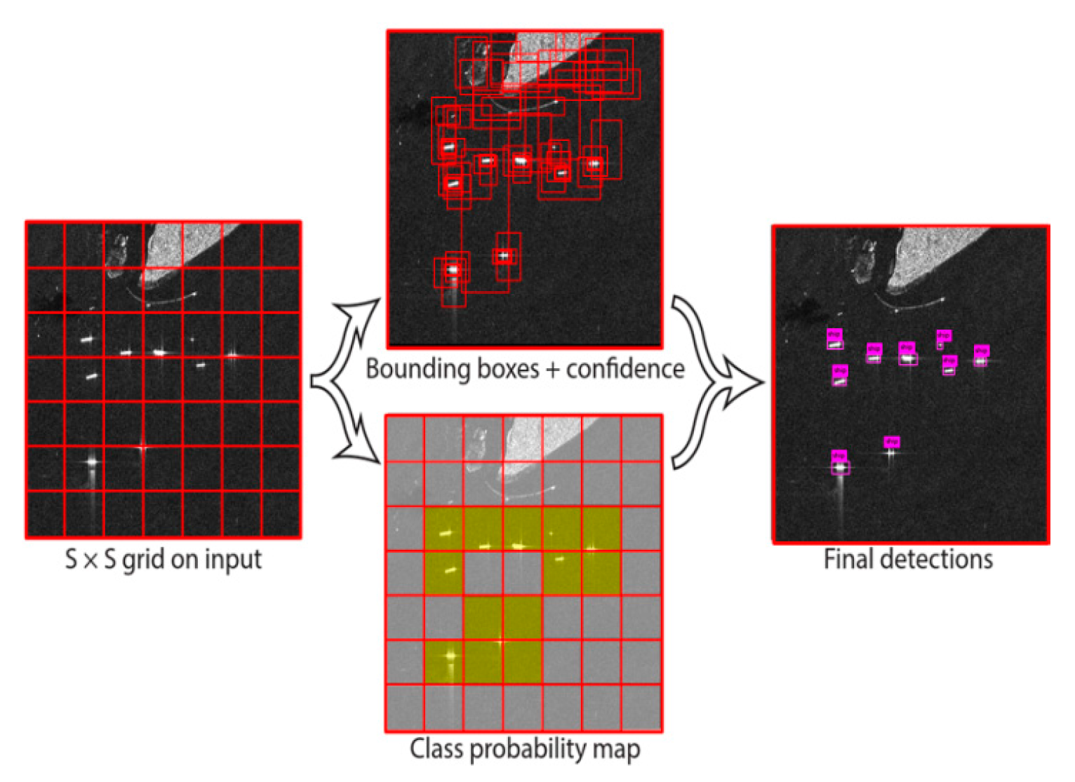
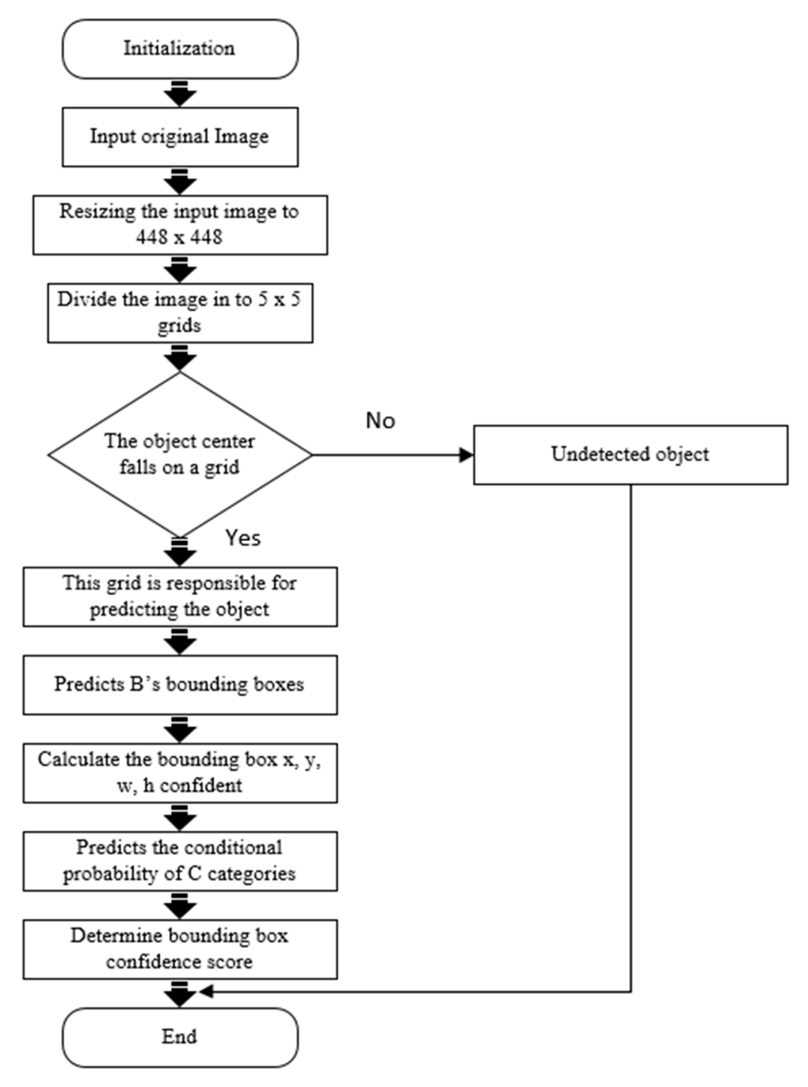
In this paper, we construct a YOLOv2-based [6] end-to-end training convolutional neural network to detect ships. First, YOLO [13] uses a single neural network to directly predict the bounding box and class probability. The SAR image is divided into an S × S grid of cells. Each grid cell predicts only one object. If the center of an object falls into a grid cell, that grid cell is responsible for detecting that object. Every grid cells predicts the B bounding boxes and the confidence score of that bounding boxes, and class probabilities. The bounding box prediction has 5 components: (x, y, w, h, confidence). The (x, y) coordinates represent the center of the box relative to the grid cell location. These coordinates are normalized to fall between 0 and 1. The (w, h) box dimensions are the width and the height of the bounding box also normalized to 0 and 1 relative to the image size.
The predicted confidence scores indicate how confident the model is that the box contains an object and also how accurate it thinks the box is that it predicts. If no object exists in that cell, the confidence scores should be zero. Otherwise, we want the confidence score to be equal to the intersection over union (IOU) between the ground truth and the predicted box [6]. Each grid cell makes B of those predictions, so there are in total S x S x B * 5 outputs related to bounding box predictions. In some cases, multiple objects can exit in a single grid cell. To solve the problem, we used the concept of anchor box. Anchor box makes it possible for the YOLOv2 algorithm to detect multiple objects centered in one grid cell. The idea of anchor box adds one more dimension to the output labels by pre-defining a number of anchor boxes. Then, we will be able to assign one object to each anchor box. Figure 1 depicted how the grids and bounding boxes are computed and looks. Figure 2 is a detection flowchart of the YOLOv2 algorithm.
Table 1 shows that there are 30 layers of YOLOv2 [6] network architecture, of which 22 layers are convolutional layers and 5 layers are the max pooling layers. The rest three layers are two route layers and one reorg layer. The route layers are performed at the 25th and 27th layers. The role of the route layer is to merge layers. For example, the 27th route is composed of layer 26 and layer 24, that is, the 26th and 24th layers are merged into the next layer. The final detection layer reorganizes the features extracted from the convolution layer to predict the probability and the bounding box of the ship. Assuming the input image size is 416×416. Table 1 depicts the size of the image after each layer operation performed. After the successive operation on each layer, the output of the 30th layer size is 13 × 13 × 30. Finally, it is reduced to a 13 × 13 size grid. The output of each grid cell is 30, i.e., (5 × 6), where 5 values refers to the 5 predictive borders for each 13 × 13 grid cell, and the 25 values (30 minus 5) refers to that each border outputs 25 values. One of the six numbers is the probability of a ship. The other five numbers are the position and size of the bounding boxes tx, ty, tw, th and the confidence of the bounding boxes.
In the object detection deep neural network, we used a pre-training model to enhance the detection performance. Visual Geometry Group-16 (VGG -16) [21] usually used as a pre-training model in many CNN versions. In YOLOv2, another pre-training model called darknet-19 is used to improve the accuracy and speed. YOLOv2 maintains almost the same accuracy as VGG-16.
YOLOv2 detection speed was at least 4 times faster than the VGG-16. Ref. [22] compared the detection performance of VGG-16 and YOLOv2 with an input image of 224×224 size. VGG-16 requires 30.69 billion floating-point operations, and GoogLeNet-based [23] YOLOv2 requires 8.52 billion floating-point operations [6]. Darknet-19 is smaller and requires only 5.58 billion floating-point operations.
3. Datasets and Experimental Results
In this section the datasets used for the purpose of the experiment, the evaluation methods used and the result discussion will be explained.
3.1. The Datasets
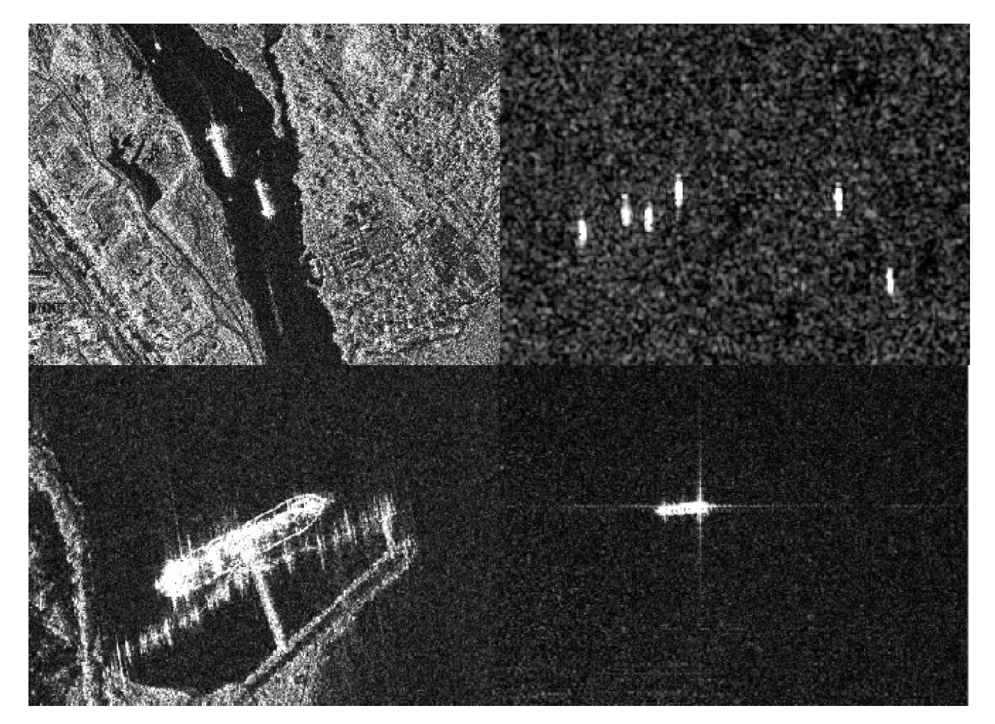
In this work, we use two types of datasets. The first dataset is SAR ship detection dataset (SSDD) [5]. SSDD dataset contains ships in different environments. This dataset is a benchmark for researchers to evaluate their approaches. In SSDD, there are a totally of 1160 images and 2456 ships. The average number of ships per image is 2.12. This vessel dataset is provided by Li et al. [5]. In the object detection task, you must manually mark the border and label of each image object’s ground truth. While PASCAL VOC already provides standardized methods of image object’s ground truth labeling. The dataset we used also follows this method to construct bounding boxes and label annotations. We divide the dataset into three parts, i.e., the training set, validation set and the testing set with the proportion of 7:2:1. The SAR images in the dataset include a variety of ships with adjacent docks and land, isolated oceans, and side by side, as shown in Figure 3.
The Second dataset, Diversified SAR Ship Detection Dataset (DSSDD), is directly collected from different sources, e.g., RadarSat-2, TerraSAR-X and Sentinel-1, with more diversity in the ships and having various SAR image resolutions. We collected 50 SAR images from those different SAR image providers. The resolution of the SAR images ranges from 1m to 5m. The SAR image sizes ranged from 1,000 × 1,000 to 15,000 × 15,000. The collected images were too large to be used by the proposed deep neural architecture, which only accepts an image with size of 416 × 416 as an input. Therefore, we segment the images into smaller sub images each with a size of 416 × 416. From the 50 large images, 1,174 sub images having a size of 416×416 were prepared. Unlike SSDD dataset where the images are rescaled to make all the ships have relatively similar sizes, we used SAR images with different resolutions and sizes to build a model directly. This gives a chance to the model be robust to any type of dataset. The dataset distribution is shown in the below Table 2.
In this paper, to annotate the SAR image, we used the LabelImg open source project on GitHub (tzutalin.github) [22], which is currently the most widely used annotation tool. LabelImg directly converts the annotation message into PASCAL VOC and ImageNet specification XML format. For all 1,174 SAR images, the image annotation was done manually. The schematic diagram of the annotated vessel is shown in Figure 4. The annotated image is used as an input to train the YOLOv2 architecture.
3.2. Evaluation Methods
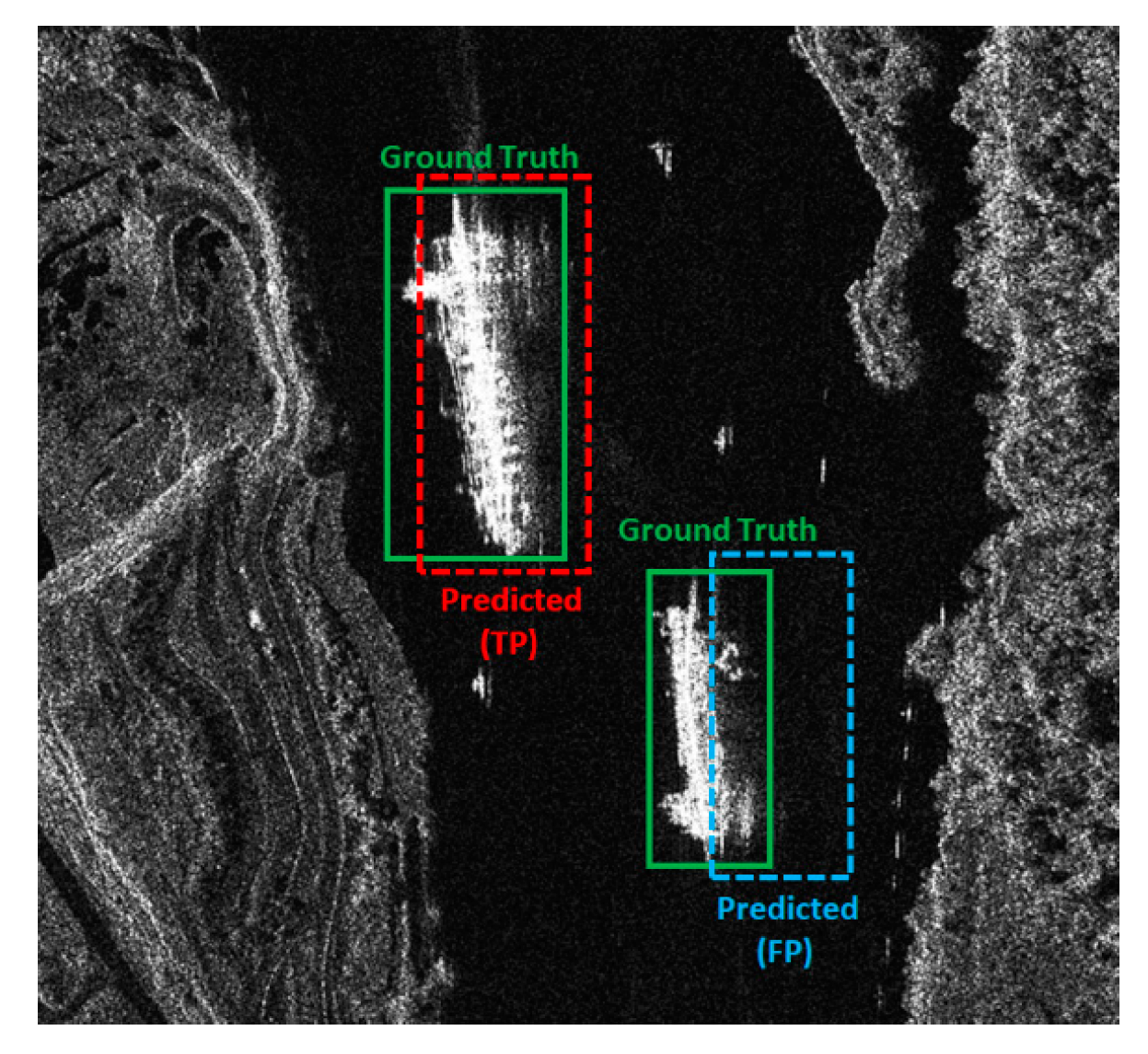
To evaluate the YOLOv2 model, the following techniques were used: IoU, accuracy and mAP. IoU is the overlap rate of the predict bounding box and ground truth generated by the model. When IoU exceeds the threshold the bounding box is considered to be correct, as shown in Equation (1). This standard is used to measure the correlation between ground truth and prediction; the higher the correlation, the higher the value. Follow-up will use IoU to calculate the average precision of our detection model. By dropping the input image into the model for prediction, the predicted bounding box of ship Bpred is obtained. However, if IoU of Bpred and Btruth is larger than the threshold value a0, and the following Equation (1) is satisfied at this time, it is regarded as a correct prediction. An example of detecting a ship in an image is shown in Figure 5. The predicted bounding box is drawn in red or blue while the ground truth bounding box is drawn in green. Our goal is to compute the IoU between predicted bounding boxes and ground truth. When IoU is greater than the 50% threshold, the test result is a true positive (TP), and the value less than threshold, it is called a false positive (FP). The false negative (FN) indicates that the model predicts that there is no ship in the image, but actually the image does contain a ship. So, we can combine these into two metrics, which are precision and recall.
IoU is frequently used as an evaluation metric to measure the accuracy of an object detector. The importance of IoU is not only limited to assigning anchor boxes during preparation of the training dataset, but is also very useful when non-max suppression algorithm is used for cleaning up whenever multiple boxes are predicted for the same object. The value of a0 is assigned to 0.5, which mean at least half of the ground truth and the predicted box cover the same region. When IoU is greater than 50% threshold, the test case is predicted as a ship.
Precision is the ratio of true positives to the identified image:
where n represents (true positives + false positives), which is the total number of photos recognized by the system.
Accuracy is the most intuitive performance measure and it is simply a ratio of correctly predicted observation to the total observations.
Recall’s denominator is true positives + false negatives. The sum of these two values can be understood as the total number (ground truth) of ships. The last evaluation method, mAP, is the area under the Recall and Precision curves. This value is between 0 and 1. Larger values of mAP represents better detection accuracy.
3.3. The Experimential Results
We trained the YOLOv2 ship detection model on two datasets. The first dataset is SSDD dataset which contains preprocessed SAR images and the ships in the images had a similar size.
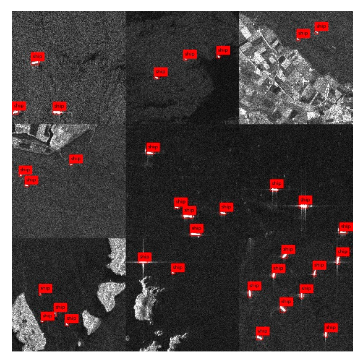
The DSSDD dataset is directly collected from different SAR image venders which have different sizes and resolutions. The dataset is a real dataset which makes the model robust to different scenarios. Figure 6 depicts some ship detection results on DSSDD dataset. The newly proposed YOLO-reduced architecture was trained on the SSDD dataset only. For the sake of fair comparison, all the experiments were performed using a PC with Intel(R) Xeon(R) E3-1226 v3 @ 3.40GHz × 24 and 64 GB of memory, NVIDIA TITAN X GPU with 12G memory and using CUDA8.0 cuDNN6.0. The operating system was 64-bit Ubuntu 16.04. We adopted a well-known open source framework, namely the Darknet framework [10], to train our deep learning models. Darknet-19 which had been pre trained on VOC 2007+2012 was selected to be the backbone of our CNN network. The results of this study verify the correctness and effectiveness of the method in both accuracy and computational cost.
From the experiment, we observed that the proposed method greatly improved the accuracy to 90.03% on the first SSDD dataset. The results are shown in Table 3.
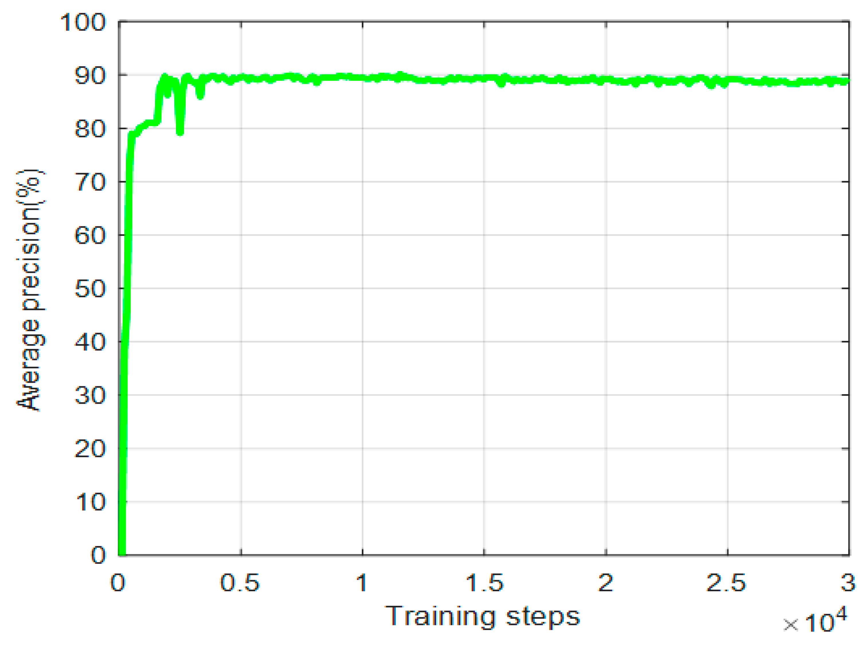
The YOLOv2 training model had a learning rate of 0.0001 and batch size of 128. As Figure 7 clearly depicts, the total training had 30,000 iterations. The average accuracy is not stable until approximately 3000 iterations. We use convolutional weights that are pre-trained on the ImageNet. Overall, this pre-trained weight is also suitable for SAR image of ships, which is helpful for the training performance of the network.
We again tested the performance of the YOLOv2 training model on another dataset, collected from the different SAR image providers with a different resolution. Unlike the SSDD dataset, the image was not rescaled to make the different resolution image have a relatively similar size, in order to make the detection much better. The results are depicted in Table 4.
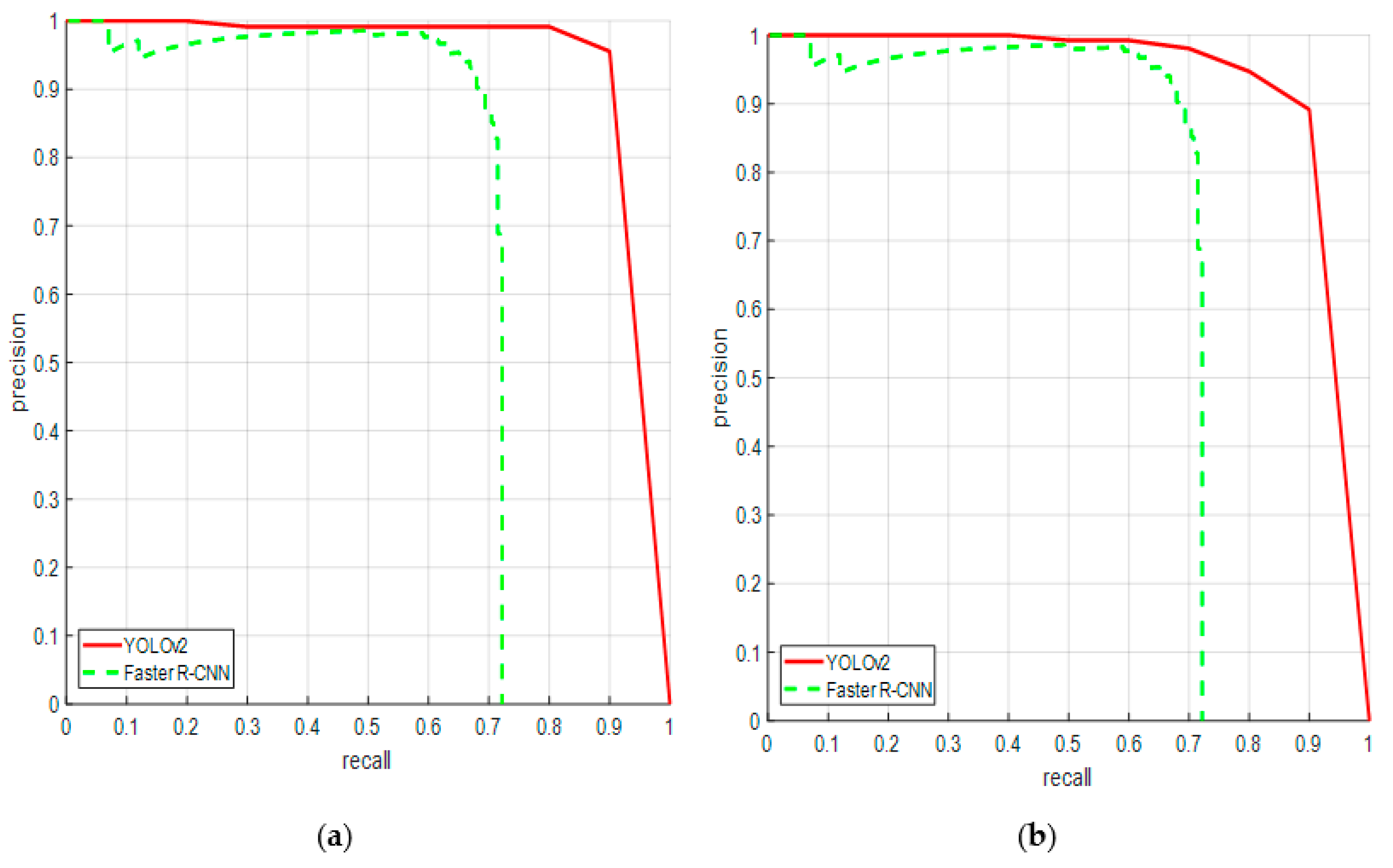
As shown in Figure 8a, YOLOv2 method had an average precision (AP) value of 90.05% on the testing set, which was higher than the 70.63% from the Faster R-CNN method on the SSDD dataset. The single-stage neural network YOLOv2 guarantees the detection speed, and has good detection performance. As shown in Figure 8b, the YOLOv2 method had an AP value of 89.13% on the testing set, which is higher than the 68.43% from the Faster R-CNN method on the DSSDD dataset.
In most cases, deep learning methods yield more promising results when a larger percent of the dataset is used as training data. We evaluated the robustness of the YOLOv2 architecture with a small number of datasets as a training dataset. For this purpose, unlike the above experiment that used 70 percent of the data to train the model, we used only 20 percent of the total data for training the architecture, and used 70 percent and 10 percent of the data for testing and validation respectively. Table 5 clearly shows the model has a good performance score even with smaller amounts of training data.
3.4. Comparing Different Image Sizes and Resolutions
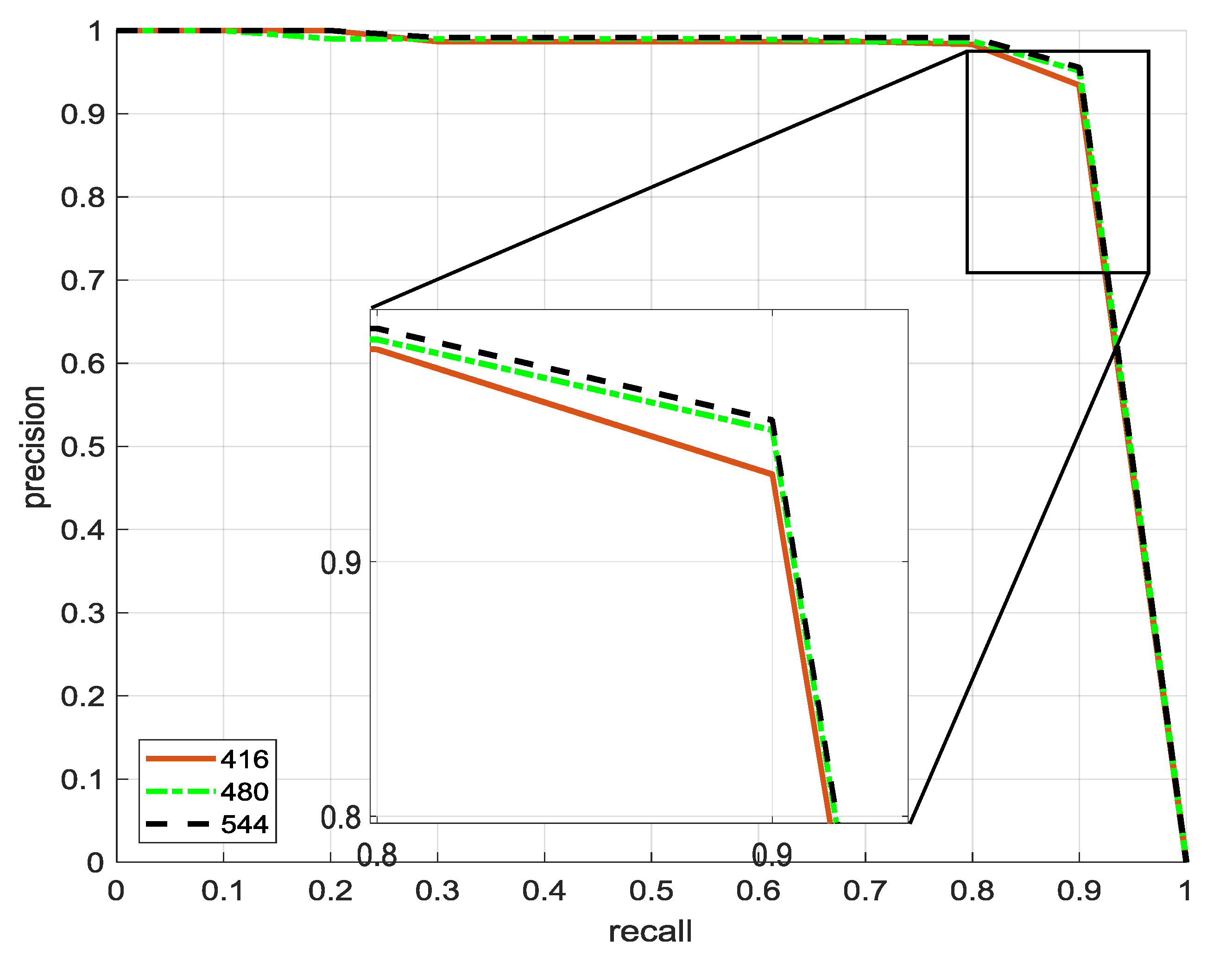
In this paper, we also tried to evaluate the performance of the YOLOv2 architecture with different image sizes and to assess the impact of image size on the detection performance of the model. For this purpose, we selected the SSDD dataset with three different image sizes 416 × 416, 480 × 480 and 544 × 544. The YOLOv2 network architecture detection performance was 89.56, 89.75 and 90.5 percent, respectively.
From the experimental results, we can see that the size of the input image to the network had a huge impact on the complexity of the convolutional neural network. Even though the detection performance was higher when the image size was increased, the average time complexity was inversely proportional to the detection performance. Table 6 depicts a detailed comparison of those different image sizes, where BFLOPS stands for billion floating point operations per second.
If the detection execution time is taken into consideration, 416×416 was the best choice. In conclusion, the greater the size of the image, the higher the average accuracy of the ship detection, but at a cost of about 1.6 times the execution time. In this study, the average accuracy was taken as the first consideration, and an image with a size of 544 × 544 was our best choice. Figure 9 shows the precision recall curves for the different image sizes. The three resolution curves are essentially overlapping because the APs of the three were very close.
Interestingly, we evaluated the YOLOv2 architecture performance with different spatial resolution images. The resolution had a direct impact on the quality of the image. If the image quality is poor, the docks, shores or canals have a tendency to appear as a ship, and that will reduce the detection rate. To make our model more robust, we collected different SAR images with various resolutions ranging from 1 m to 5 m. In reality, the SAR images provided had different resolutions. To make our model suitable for all different SAR images in real time, we used SAR images with different resolutions as the training data for our model. We conducted the experiments with 10 SAR images from each sensor type as the testing datasets. The first 10 images were tested from a sentinel-1 sensor, with a resolution of 5 m. The second 10 SAR images that were tested were from a TerraSAR-X sensor, which has a resolution of 1 m. The experimental results in Table 7 show that the resolution of SAR images and their detection performance are inversely proportional.
From the experimental results, we can see that the YOLOv2 model required less computational time than the faster RCNN. The model’s computational time was not similar on both datasets. The YOLOv2 computational time on the DSSDD dataset was bigger than the SSDD dataset. In this paper, we applied a preprocessing stage that divided the large image into smaller sizes to make the detection more convenient for the model. It is possible to estimate the execution time for more realistic SAR dataset dimensions. The larger the SAR image, the greater the execution time.
3.5. Network Optimization
In this research, besides evaluating the performance of the state of the art detection method on SAR imagery, we developed our own new architecture that has less layers. In YOLOv2, the route layer is a feature map that combines the features of the underlying convolutional layer (with large features) and the previous layer of convolutional layers. The Reorg (reorganization) layer is used to reorganize the feature map size so that the route layer is the same size as the convolution layer to be added.
In order to effectively improve the performance of the ship detection problem, we examined the nature of ships with respect to the background. The size of the ship is much smaller than the size of the whole picture. The size of a ship is 52 × 5 pixels, which only accounts for 0.09% of the picture in a picture of 544 × 544 pixels. Thus, compared to the size of the whole image, the ship size is too small. So, suitable network architectures must be designed to find more effective features.
4. YOLOv2-Reduced Architecture
YOLOv2-reduced architecture reduces some of the top layers of the YOLOv2 architecture. The repetitive convolution layer was not very effective for ship detection (i.e., convolutional layers 23, 24, 25). Since the ship is relatively insignificant to the ocean, applying this consecutive convolution is not required. Therefore, we reduced these three convolutional layers to one layer.
This approach reduces the time complexity of YOLOv2 architecture with almost competitive detection performance. Table 8 depicts the numbers and types of layers in the YOLOv1, YOLOv2 and YOLOv2-reduced network architectures. The experimental results show that YOLOv2-reduced network architecture was better than the YOLOv2 in terms of computational time. Table 9 shows the average accuracy and speed of the two architectures on the SSDD dataset.
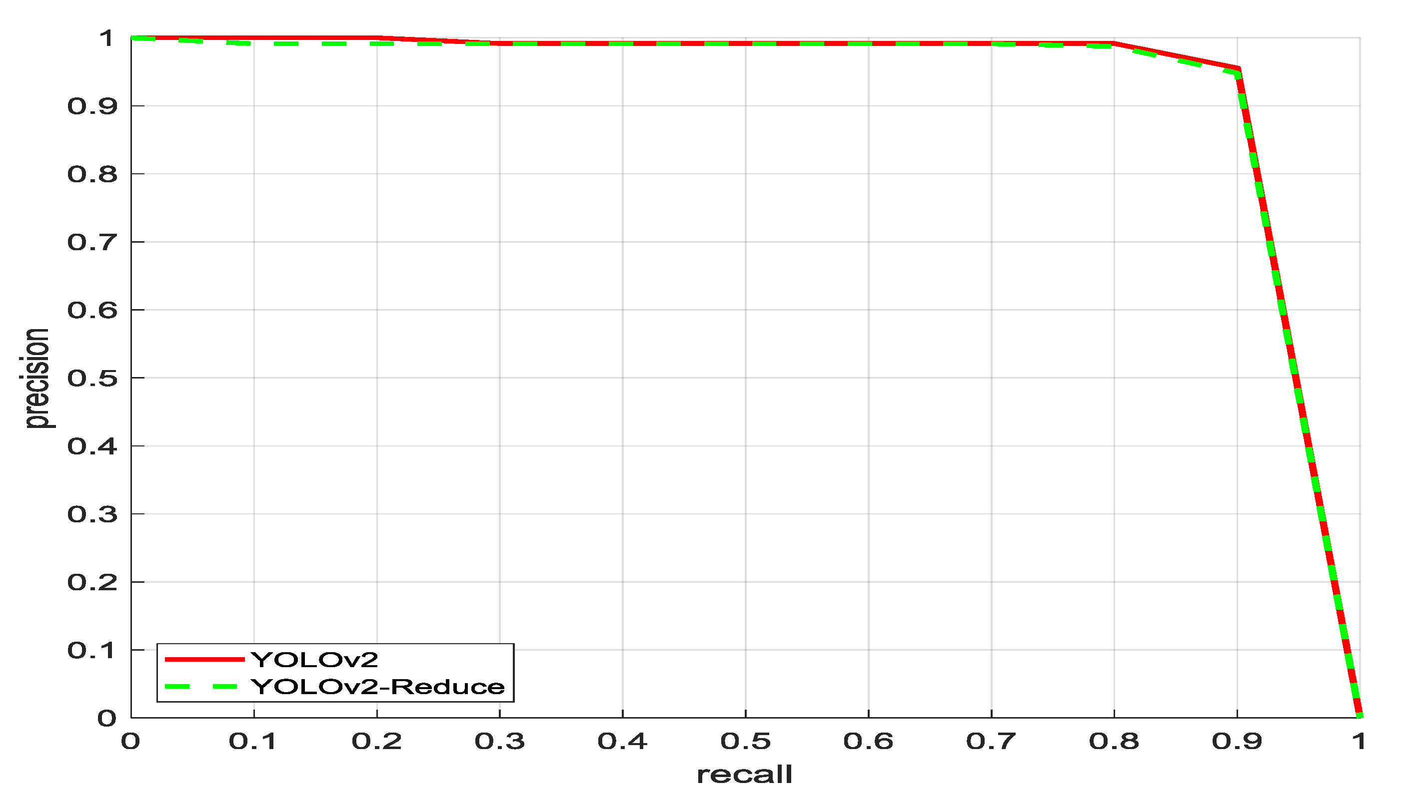
The experimental results show that reducing the repeated convolutional layer, YOLOv2-reduced, did not improve the average accuracy as shown in Figure 10. In the precision recall curve the YOLOv2-reduced architecture covered almost the same area as the YOLOv2 graph. However, it greatly reduced the overall detection time.
5. Conclusions
In this paper, we evaluated the performance of the YOLOv2 deep network architecture to detect a vessel in various scenarios. The experimental results on a basic SAR image dataset show that the YOLOv2 method outperforms current technologies in terms of accuracy and performance in near real-time, especially in complex situations. In the faster-R-CNN identification experience, we found that errors often occurred in the same phase as the terrestrial phase in neighboring images, such as docks, shores or canals. They are the main areas of lowered accuracy. According to this study, YOLOv2 is very suitable for SAR image ship detection and its detection speed is 5.8 times faster than faster-R-CNN. From the experimental results, we can clearly show that the YOLOv2 architecture has better detection accuracy and speed than the other recent detection methods on both datasets. Although YOLOv2 architecture has a better detection performance and speed, we thought this speed is not enough for real time detection systems. Therefore, in this paper, we introduced a new network architecture, YOLOv2-reduced, which has a better detection time than the YOLOv2 network on a NVIDIA TITAN X GPU. The performance of the proposed method was evaluated on the SSDD dataset. It showed a 2.5 times better detection time than YOVOv2, with a competent detection accuracy.
Author Contributions
Conceptualization, W.-H.L.; Data curation, C.-Y.H.; Methodology, Y.-L.C., and C.-Y.H.; Supervision, Y.-L.C.; Validation, A.A.; Writing—review & editing, A.A., L.C. and Y.C.W.
Funding
This work was partially sponsored by the Ministry of Science and Technology of Taiwan, under Grant Nos: MOST 107-2116-M-027-003 and MOST 107-2221-E-019-028, and National Taipei University of Technology and National Taiwan Ocean University under Grant No: USTP-NTUT-NTOU-107-02.
Conflicts of Interest
The authors declare no conflicts of interest.
References
- Krizhevsky, A.; Sutskever, I.; Hinton, G. Imagenet classification with deep convolutional neural networks. In Advances in Neural Information Processing Systems; ACM: New York, NY, USA, 2012; pp. 1097–1105. [Google Scholar] [CrossRef]
- Dahl, G.E.; Yu, D.; Deng, L.; Acero, A. Context-Dependent Pre-Trained Deep Neural Networks for Large-Vocabulary Speech Recognition. IEEE Trans. Audio Lang. Process. 2012, 20, 30–42. [Google Scholar] [CrossRef] [Green Version]
- Cireşan, D.C.; Meier, U.; Gambardella, L.M.; Schmidhuber, J. Deep, Big, Simple Neural Nets for Handwritten Digit Recognition. Neural Comput. 2010, 22, 3207–3220. [Google Scholar] [CrossRef] [PubMed] [Green Version]
- Raina, R.; Madhavan, A.; Ng, A.Y. Large-scale deep unsupervised learning using graphics processors. In Proceedings of the 26th Annual International Conference on Machine Learning, Montreal, QC, Canada, 14–18 June 2009; pp. 1–8. [Google Scholar]
- Li, J.; Qu, C.; Shao, J. Ship detection in SAR images based on an improved faster R-CNN. In Proceedings of the 2017 SAR in Big Data Era: Models, Methods and Applications (BIGSARDATA), Beijing, China, 13–14 November 2017; pp. 1–6. [Google Scholar]
- Redmon, J.; Farhadi, A. YOLO9000: Better, Faster, Stronger. In Proceedings of the 2017 IEEE Conference on Computer Vision and Pattern Recognition (CVPR), Honolulu, HI, USA, 21–26 July 2017; pp. 6517–6525. [Google Scholar]
- Girshick, R.; Donahue, J.; Darrell, T.; Malik, J. Rich Feature Hierarchies for Accurate Object Detection and Semantic Segmentation. In Proceedings of the 2014 IEEE Conference on Computer Vision and Pattern Recognition (CVPR), Columbus, OH, USA, 23–28 June 2014; pp. 580–587. [Google Scholar]
- Girshick, R. Fast R-CNN. In Proceedings of the 2015 IEEE International Conference on Computer Vision (ICCV), Santiago, Chile, 13–16 December 2015; pp. 1440–1448. [Google Scholar]
- Uijlings, J.R.R.; van de Sande, K.E.A.; Gevers, T.; Smeulders, A.W.M. Selective Search for Object Recognition. Int. J. Comput. Vis. 2011, 104, 154–171. [Google Scholar] [CrossRef]
- Ren, S.; He, K.; Girshick, R.; Sun, J. Faster R-CNN: Towards Real-Time Object Detection with Region Proposal Networks. In Advances in Neural Information Processing Systems; IEEE: New York, NY, USA, 2015; pp. 91–99. [Google Scholar] [CrossRef]
- Zhang, J.; Huang, M.; Jin, X.; Li, X. A Real-Time Chinese Traffic Sign Detection Algorithm Based on Modified YOLOv2. Algorithms 2017, 10, 127. [Google Scholar] [CrossRef]
- Everingham, M.; van Gool, L.; Williams, C.K.; Winn, J.; Zisserman, A. The Pascal Visual Object Classes (VOC) Challenge. Int. J. Comput. Vis. 2010, 88, 303–338. [Google Scholar] [CrossRef]
- Redmon, J.; Divvala, S.; Girshick, R.; Farhadi, A. You Only Look Once: Unified, Real-Time Object Detection. In Proceedings of the 2016 IEEE Conference on Computer Vision and Pattern Recognition (CVPR), Las Vegas, NV, USA, 27–30 June 2016; pp. 779–788. [Google Scholar]
- Crisp, D.J. The State-of-Art in Ship Detection in Synthetic Aperture Radar Imagery. In Proceedings of the 12th Australasian Remote Sensing and Photogrammetry Conference, Fremantle, Western Australia, 18–22 October 2004; ISBN 0958136610. [Google Scholar]
- Iervolino, P.; Guida, R. A Novel Ship Detector Based on the Generalized-Likelihood Ratio Test for SAR Imagery. IEEE J. Sel. Topics Appl. Earth Observ. Remote Sens. 2017, 10, 3616–3630. [Google Scholar] [CrossRef] [Green Version]
- Leng, X.; Ji, K.; Yang, K.; Zou, H. A bilateral CFAR algorithm for ship detection in SAR images. IEEE Geosci. Remote Sens. Lett. 2015, 12, 1536–1540. [Google Scholar] [CrossRef]
- Greidanus, H.; Alvarez, M.; Santamaria, C.; Thoorens, F.; Kourti, N.; Argentieri, P. The SUMO Ship Detector Algorithm for Satellite Radar Images. Remote Sens. 2017, 9, 246. [Google Scholar] [CrossRef]
- Iervolino, P.; Guida, R.; Whittaker, P. A novel ship-detection technique for Sentinel-1 SAR data. In Proceedings of the 2015 IEEE 5th Asia-Pacific Conference on Synthetic Aperture Radar (APSAR), Singapore, 1–4 September 2015; pp. 797–801. [Google Scholar]
- Marino, A.; Iervolino, P. Ship detection with Cosmo-SkyMed PINGPONG data using the dual-pol ratio anomaly detector. In Proceedings of the 2017 IEEE International Geoscience and Remote Sensing Symposium (IGARSS), Fort Worth, TX, USA, 23–28 July 2017; pp. 3897–3900. [Google Scholar]
- Marino, A.; Dierking, W.; Wesche, C. A Depolarization Ratio Anomaly Detector to Identify Icebergs in Sea Ice Using Dual-Polarization SAR Images. IEEE Trans. Geosci. Remote Sens. 2016, 54, 5602–5615. [Google Scholar] [CrossRef]
- Simonyan, K.; Zisserman, A. Very Deep Convolutional Networks for Large-Scale Image Recognition. In Proceedings of the 3rd International Conference on Learning Representations (ICLR), San Diego, CA, USA, 7–9 May 2015. [Google Scholar]
- Tzutalin. Available online: https://github.com/tzutalin/labelImg (accessed on 6 July 2018).
- Szeged, C.; Liu, W.; Jia, Y.; Sermanet, P.; Reed, S.; Anguelov, D.; Erhan, D.; Vanhoucke, V.; Rabinovich, A. Going Deeper with Convolutions. In Proceedings of the IEEE Conference on Computer Vision and Pattern Recognition (CVPR), Boston, MA, USA, 7–12 June 2015; pp. 1–9. [Google Scholar]
Figure 1.
You Only Look Once (YOLO) system model detection as a regression problem. First partition the image into an S * S grid and for each grid cell the model predicts B bounding boxes, confidence for those boxes, and C class probabilities [6].
Figure 1.
You Only Look Once (YOLO) system model detection as a regression problem. First partition the image into an S * S grid and for each grid cell the model predicts B bounding boxes, confidence for those boxes, and C class probabilities [6].

Figure 2.
YOLOv2 detection flowchart.

Figure 3.
Sample images from the SAR ship detection dataset (SSDD) dataset [7].
Figure 3.
Sample images from the SAR ship detection dataset (SSDD) dataset [7].

Figure 4.
Sample labeling of ship using LabelImg software.

Figure 5.
Example of calculate intersection over union (IOU).

Figure 6.
Examples of ship detection in different cases.

Figure 7.
Training average precision for each iteration in class of ship on SSDD.

Figure 8.
(a) Precision recall curve performance of ship detection on SSDD (b) Precision recall curve performance of ship detection on the DSSDD dataset.
Figure 8.
(a) Precision recall curve performance of ship detection on SSDD (b) Precision recall curve performance of ship detection on the DSSDD dataset.

Figure 9.
Precision recall curve for different image sizes using YOLOv2.

Figure 10.
Precision recall curve for YOLOv2 and YOLOv2-reduced on the SSDD dataset.


Table 1.
You Only Look Once version 2 (YOLOv2) Network Architecture.
| No. | Type | Input | Filters | Size/Stride | Output |
|---|---|---|---|---|---|
| 0 | conv | 416 × 416 × _3 | _32 | 3 × 3/1 | 416 × 416 × __32 |
| 1 | max | 416 × 416 × _32 | 2 × 2/2 | 208 × 208 × _32 | |
| 2 | conv | 208 × 208 × _32 | _64 | 3 × 3/1 | 208 × 208 × _64 |
| 3 | max | 208 × 208 × _64 | 2 × 2/2 | 104 × 104 × _64 | |
| 4 | conv | 104 × 104 × _64 | _128 | 3 × 3/1 | 104 × 104 × _128 |
| 5 | conv | 104 × 104 × _128 | _64 | 1 × 1/1 | 104 × 104 × _64 |
| 6 | conv | 104 × 104 × _64 | _128 | 3 × 3/1 | 104 × 104 × _128 |
| 7 | max | 104 × 104 × _128 | 2 × 2/2 | _52 × _52 × _128 | |
| 8 | conv | _52 × _52 × _128 | _256 | 3 × 3/1 | _52 × _52 × _256 |
| 9 | conv | _52 × _52 × _256 | _128 | 1 × 1/1 | _52 × _52 × _128 |
| 10 | conv | _52 × _52 × _128 | _256 | 3 × 3/1 | _52 × _52 × _256 |
| 11 | max | _52 × _52 × _256 | 2 × 2/2 | _26 × _26 × _256 | |
| 12 | conv | _26 × _26 × _256 | _512 | 3 × 3/1 | _26 × _26 × _512 |
| 13 | conv | _26 × _26 × _512 | _256 | 1 × 1/1 | _26 × _26 × _256 |
| 14 | conv | _26 × _26 × _256 | _512 | 3 × 3/1 | _26 × _26 × _512 |
| 15 | conv | _26 × _26 × _512 | _256 | 1 × 1/1 | _26 × _26 × _256 |
| 16 | conv | _26 × _26 × _256 | _512 | 3 × 3/1 | _26 × _26 × _512 |
| 17 | max | _26 × _26 × _512 | 2 × 2/2 | _13 × _13 × _512 | |
| 18 | conv | _13 × _13 × _512 | 1024 | 3 × 3/1 | _13 × _13 × 1024 |
| 19 | conv | _13 × _13 × 1024 | _512 | 1 × 1/1 | _13 × _13 × _512 |
| 20 | conv | _13 × _13 × _512 | 1024 | 3 × 3/1 | _13 × _13 × 1024 |
| 21 | conv | _13 × _13 × 1024 | _512 | 1 × 1/1 | _13 × _13 × _512 |
| 22 | conv | _13 × _13 × _512 | 1024 | 3 × 3/1 | _13 × _13 × 1024 |
| 23 | conv | _13 × _13 × 1024 | 1024 | 3 × 3/1 | _13 × _13 × 1024 |
| 24 | conv | _13 × _13 × 1024 | 1024 | 3 × 3/1 | _13 × _13 × 1024 |
| 25 | route | 16th | _26 × _26 × _512 | ||
| 26 | reorg | _26 × _26 × _512 | _ × _/1 | _13 × _13 × 2048 | |
| 27 | route | 26th and 24th | _13 × _13 × 3072 | ||
| 28 | conv | _13 × _13 × 3072 | 1024 | 3 × 3/1 | _13 × _13 × 1024 |
| 29 | conv | _13 × _13 × 1024 | 30 | 1 × 1/1 | _13 × _13 × _30 |
Table 2.
Diversified SAR Ship Detection Dataset (DSSDD) dataset distribution.
| Data Sets | Number of Samples |
|---|---|
| Training Set | 822 |
| Validation Set | 235 |
| Testing set | 117 |
| Total | 1174 |
Table 3.
Ship Detection Accuracy and Speed Comparison on SSDD.
| Networks | Accuracy | Time Per Image (ms) |
|---|---|---|
| Faster-R-CNN | 70.63% | 206 |
| YOLOv2 | 90.05% | 25 |
Table 4.
Ship Detection Accuracy and Speed Comparison on the DSSDD Dataset.
| Networks | Accuracy | Time Per Image (ms) |
|---|---|---|
| Faster-R-CNN | 68.43% | 221 |
| YOLOv2 | 89.13% | 27 |
Table 5.
The performance of YOLOv2 architecture with various training and testing data compositions.
Table 5.
The performance of YOLOv2 architecture with various training and testing data compositions.
| Networks | Dataset | Accuracy | Time Per Image (ms) |
|---|---|---|---|
| 70% training; 20% testing | SSDD | 90.05% | 25 |
| DSSDD | 89.13% | 27 | |
| 20% training; 70% testing | SSDD | 80.74% | 25 |
| DSSDD | 68.5% | 27 |
Table 6.
Evaluate the Performance of YOLOv2 with Different Image size.
| Method | Image Size | Avg. IOU | AP | Avg. Time (ms) | BFLOPS |
|---|---|---|---|---|---|
| YOLOv2 | 416 × 416 | 75.24 | 89.56 | 15.718 | 29.338 |
| 480 × 480 | 76.99 | 89.79 | 17.545 | 39.060 | |
| 544 × 544 | 78.2 | 90.05 | 25.767 | 50.170 |
Table 7.
YOLOv2 performance with different resolutions.
| Sensors Types | Resolution | Accuracy % |
|---|---|---|
| Sentinel-1 | 5 m | 89.29% |
| TerraSAR-X | 1 m | 90.47% |
Table 8.
The Network Architectures of YOLOv2 and YOLOv2-reduced.
| YOLOv1 | YOLOv2 | YOLOv2-Reduced |
|---|---|---|
| Conv7/2-64 | Conv3-32 | Conv3-32 |
| Maxpool/2 | Maxpool/2 | Maxpool/2 |
| Conv3-192 | Conv3-64 | Conv3-64 |
| Maxpool/2 | Maxpool/2 | Maxpool/2 |
| Conv1-128 | Conv3-128 | Conv3-128 |
| Conv3-256 | Conv1-64 | Conv1-64 |
| Conv1-256 | Conv3-128 | Conv3-128 |
| Conv3-512 | Maxpool/2 | Maxpool/2 |
| Maxpool/2 | Conv3-256 | Conv3-256 |
| Conv1-256 | Conv1-128 | Conv1-128 |
| Conv3-512 | Conv3-256 | Conv3-256 |
| Conv1-256 | Maxpool/2 | Maxpool/2 |
| Conv3-512 | Conv3-512 | Conv3-512 |
| Conv1-256 | Conv1-256 | Conv1-256 |
| Conv3-512 | Conv3-512 | Conv3-512 |
| Conv1-256 | Conv1-256 | Conv1-256 |
| Conv3-512 | Conv3-512 | Conv3-512 |
| Conv1-512 | Maxpool/2 | Maxpool/2 |
| Conv3-1024 | Conv3-1024 | Conv3-1024 |
| Maxpool/2 | Conv1-512 | Conv1-512 |
| Conv1-512 | Conv3-1024 | Conv3-1024 |
| Conv3-1024 | Conv1-512 | Conv1-512 |
| Conv1-512 | Conv3-1024 | Conv3-1024 |
| Conv3-1024 | Conv3-1024 | Route |
| Conv3-1024 | Conv3-1024 | Conv1(64) |
| Conv3/2-1024 | Route | Reorg/Route |
| Conv3-1024 | Conv1(64) | Conv3-1024 |
| Conv3-1024 | Reorg/Route | Conv1 |
| Local | Conv3-1024 | Detection |
| Dropout | Conv1 | |
| Conn | Detection | |
| Detection |
Table 9.
Average Accuracy and Speed Comparison between YOLOv2 and YOLOv2-reduced Architectures.
| Method | AP | Avg. Time (ms) | BFLOPS |
|---|---|---|---|
| YOLOv2 | 90.05 | 25.767 | 50.17 |
| YOLOv2-reduced | 89.76 | 10.937 | 44.72 |
© 2019 by the authors. Licensee MDPI, Basel, Switzerland. This article is an open access article distributed under the terms and conditions of the Creative Commons Attribution (CC BY) license (http://creativecommons.org/licenses/by/4.0/).
Share and Cite
MDPI and ACS Style
Chang, Y.-L.; Anagaw, A.; Chang, L.; Wang, Y.C.; Hsiao, C.-Y.; Lee, W.-H. Ship Detection Based on YOLOv2 for SAR Imagery. Remote Sens. 2019, 11, 786. https://0-doi-org.brum.beds.ac.uk/10.3390/rs11070786
AMA Style
Chang Y-L, Anagaw A, Chang L, Wang YC, Hsiao C-Y, Lee W-H. Ship Detection Based on YOLOv2 for SAR Imagery. Remote Sensing. 2019; 11(7):786. https://0-doi-org.brum.beds.ac.uk/10.3390/rs11070786
Chicago/Turabian StyleChang, Yang-Lang, Amare Anagaw, Lena Chang, Yi Chun Wang, Chih-Yu Hsiao, and Wei-Hong Lee. 2019. "Ship Detection Based on YOLOv2 for SAR Imagery" Remote Sensing 11, no. 7: 786. https://0-doi-org.brum.beds.ac.uk/10.3390/rs11070786
Note that from the first issue of 2016, this journal uses article numbers instead of page numbers. See further details here.