Across Date Species Detection Using Airborne Imaging Spectroscopy

 , , , ,
Abstract
:1. Introduction
2. Materials and Methods
2.1. Study Site
2.2. Hyperspectral Data
2.3. Statistically Based Spectral Data Pre-Processing
2.3.1. Mean Filtering
2.3.2. Spectrum Normalisation
2.4. Physically Based Spectral Data Pre-Processing
2.4.1. Atmospheric Corrections
2.4.2. Shadow Removal
2.4.3. Bidirectional Reflectance Distribution Function
2.4.4. Impact of Flight Line Overlap
2.5. Data Analysis
2.5.1. Variance Analysis
2.5.2. Classification
2.5.3. Classification Strategy
2.5.4. Spectral Stability Analysis
3. Results
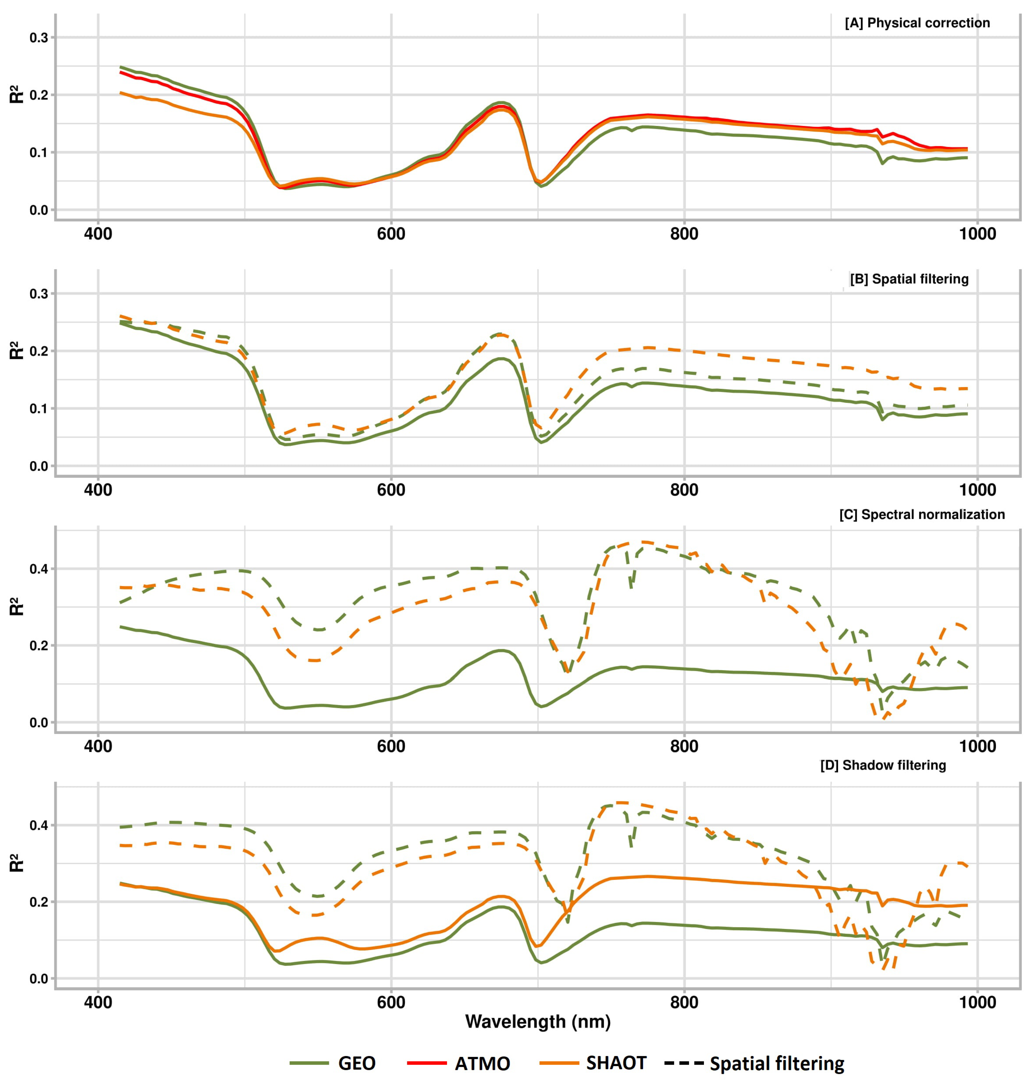
3.1. Variance Analysis
3.2. Discriminant Analysis
3.2.1. First Setting (Single Date)
3.2.2. Second Setting (Cross Date Training and Validation)
3.3. Comparing ANOVA and LDA Results
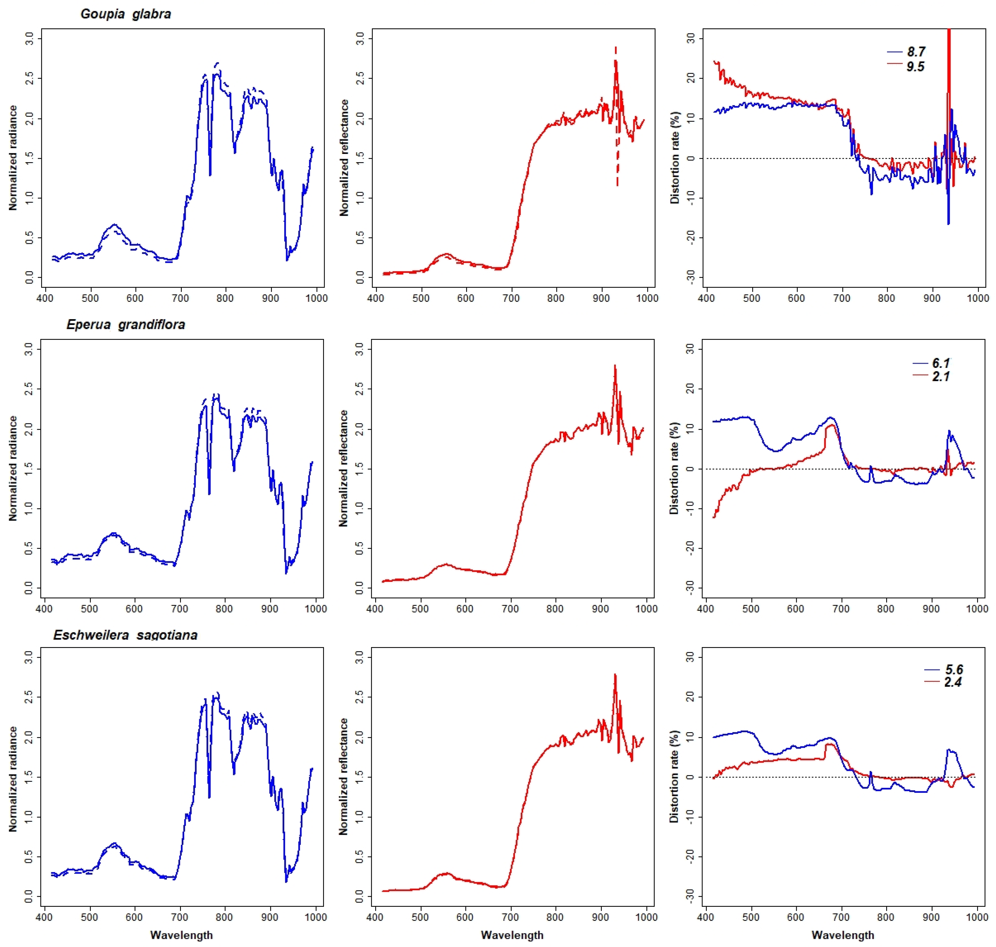
3.4. Spectral Stability Analysis
4. Discussion
4.1. LDA Classification Accuracy
4.2. Simple Methods
4.3. Operational Setting
5. Conclusions
Author Contributions
Funding
Acknowledgments
Conflicts of Interest
Abbreviations
| CIRAD | Centre de coopération internationale en recherche agronomique pour le développement |
| LiDAR | Light Detection And Ranging |
| RGB | Red, Green, Blue |
| ITC | individual tree crowns |
| DSM | Digital Surface Model |
| WGS | World Geodetic System |
| UTM | Universal Transverse Mercator |
| EPSG | European Petroleum Survey Group |
| APDA | Atmospheric Precorrected Differential Absorption |
| AOT | Aerosol Optical Thickness |
| SHAOT | shadow-based AOT |
| BRDF | bidirectional reflectance distribution function |
| SNR | Signal to Noise Ratio |
| LDA | Linear Discriminant Analysis |
| SVM | Support Vector Machine |
| RBF | Radial Basic function |
| SWIR | Short-Wave Infrared |
Appendix A

| Treatment | Spectral Average | Majority Vote | ||
|---|---|---|---|---|
| Accuracy (%) | Kappa (%) | Accuracy (%) | Kappa (%) | |
| L1b | 79.4 | 76.2 | 75.5 | 70.6 |
| L1b Spa.F | 79.6 | 76.4 | 81.7 | 78.9 |
| L1b Spa.F, norm. | 81.7 | 79.0 | 83 | 80.5 |
| L1b Spa.F, norm., Sha.R | 81.7 | 79.0 | 83.3 | 80.9 |
| L1c without SHAOT | 79.1 | 75.7 | 74.3 | 68.9 |
| L1c with SHAOT | 79.2 | 75.9 | 75.3 | 70.3 |
| L1c SHAOT, Spa.F | 79.2 | 75.9 | 81.9 | 79.1 |
| L1c Spa.F, SHAOT | 79.4 | 76.2 | 82.0 | 79.3 |
| L1c SHAOT, Sha.R | 79.7 | 76.5 | 76.5 | 71.9 |
| L1c Spa.F, SHAOT, norm. | 81.3 | 78.5 | 82.7 | 80.1 |
| L1c Spa.F, SHAOT, Sha.R | 79.7 | 76.5 | 82.6 | 80.0 |
| L1c Spa.F, SHAOT, norm., Sha.R | 81.4 | 78.6 | 83.2 | 80.8 |
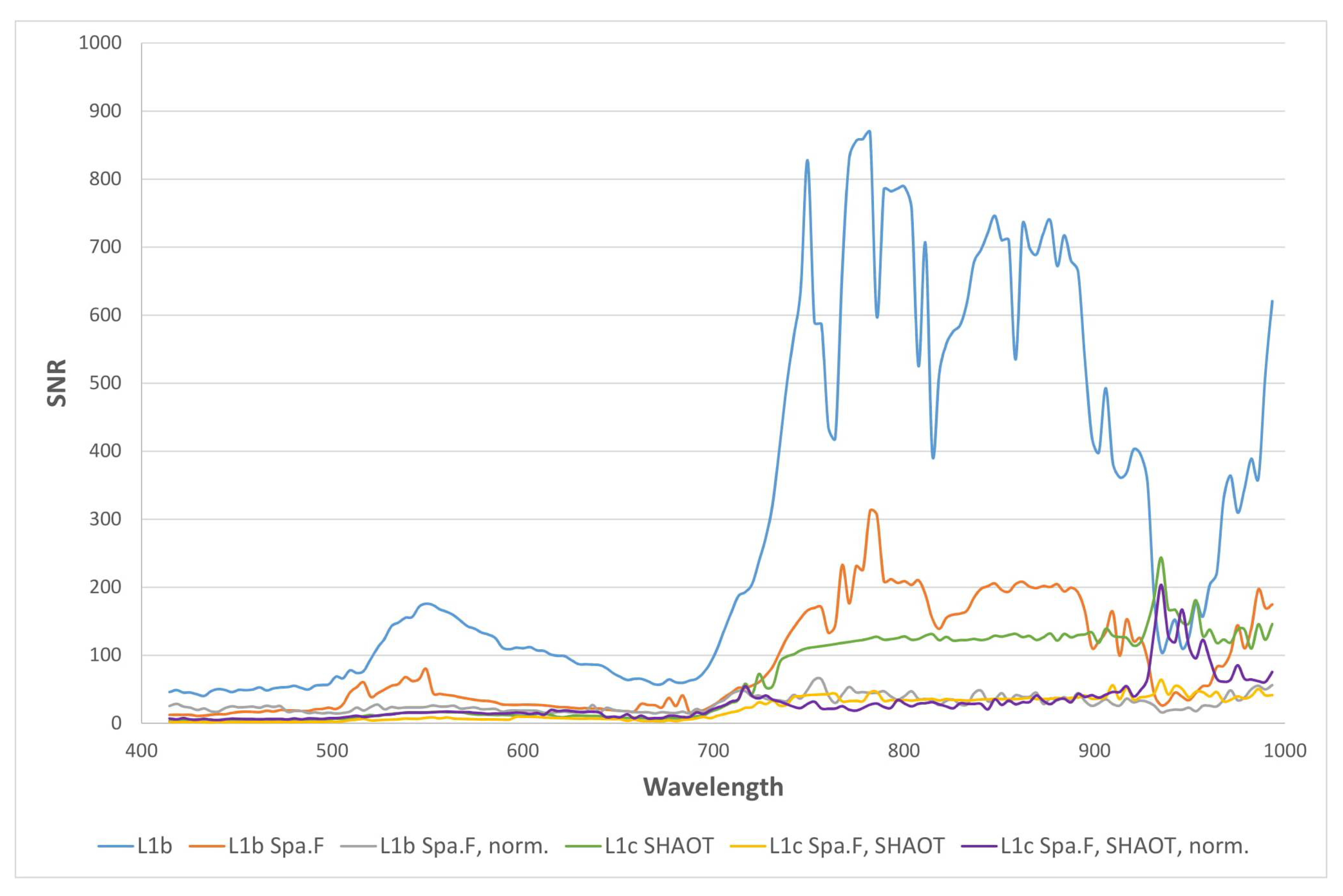
Appendix B

- Search for the 7 × 7 pixels patch with smallest noise throughout the whole image in each band.
- Calculate the mean of the whole image and the mean of the patch
- Calculate the noise in the found patch after high pass filtering
- Obtain SNR values as mean reflectance divided by the noise in the patch
Appendix C
| Treatment | Pixel | Object | ||
|---|---|---|---|---|
| Accuracy (%) | Kappa (%) | Accuracy (%) | Kappa (%) | |
| L1b Spa,F, norm, | 56.4 | 21.5 | 59.0 | 40.7 |
| L1c Spa,F, SHAOT, norm, | 58.3 | 28.2 | 61.7 | 46.8 |
| L1b Spa,F, norm., Sha,R | 57.3 | 25.4 | 60.3 | 44.0 |
| L1c Spa,F, SHAOT, norm., Sha,R | 59.3 | 32.6 | 62.4 | 48.6 |
Appendix D
References
- Ter Steege, H.; Pitman, N.C.A.; Sabatier, D.; Baraloto, C.; Salomao, R.P.; Guevara, J.E.; Phillips, O.L.; Castilho, C.V.; Magnusson, W.E.; Molino, J.F.; et al. Hyperdominance in the Amazonian Tree Flora. Science 2013, 342, 1243092. [Google Scholar] [CrossRef]
- Brienen, R.J.W.; Phillips, O.L.; Feldpausch, T.R.; Gloor, E.; Baker, T.R.; Lloyd, J.; Lopez-Gonzalez, G.; Monteagudo Mendoza, A.; Malhi, Y.; Lewis, S.L.; et al. Long-term decline of the Amazon carbon sink. Nature 2014, 519, 344–348. [Google Scholar] [CrossRef]
- Barlow, J.; França, F.; Gardner, T.A.; Hicks, C.C.; Lennox, G.D.; Berenguer, E.; Castello, L.; Economo, E.P.; Ferreira, J.; Guénard, B.; et al. The future of hyperdiverse tropical ecosystems. Nature 2018, 559, 517–526. [Google Scholar] [CrossRef]
- DRYFLOR; Banda, K.; Delgado-Salinas, A.; Dexter, K.G.; Linares-Palomino, R.; Oliveira-Filho, A.; Prado, D.; Pullan, M.; Quintana, C.; Riina, R.; et al. Plant diversity patterns in neotropical dry forests and their conservation implications. Science 2016, 353, 1383–1387. [Google Scholar] [CrossRef] [Green Version]
- McDowell, N.; Allen, C.D.; Anderson-Teixeira, K.; Brando, P.; Brienen, R.; Chambers, J.; Christoffersen, B.; Davies, S.; Doughty, C.; Duque, A.; et al. Drivers and mechanisms of tree mortality in moist tropical forests. New Phytol. 2018, 219, 851–869. [Google Scholar] [CrossRef] [Green Version]
- O’Neill, D.W.; Fanning, A.L.; Lamb, W.F.; Steinberger, J.K. A good life for all within planetary boundaries. Nat. Sustain. 2018, 1, 88–95. [Google Scholar] [CrossRef]
- Deininger, K.; Byerlee, D. Rising Global Interest in Farmland: Can It Yield Sustainable and Equitable Benefits? The World Bank: Washington, DC, USA, 2011. [Google Scholar] [CrossRef]
- Alamgir, M.; Campbell, M.J.; Sloan, S.; Goosem, M.; Clements, G.R.; Mahmoud, M.I.; Laurance, W.F. Economic, Socio-Political and Environmental Risks of Road Development in the Tropics. Curr. Biol. 2017, 27, R1130–R1140. [Google Scholar] [CrossRef]
- Mitchard, E.T.A.; Feldpausch, T.R.; Brienen, R.J.W.; Lopez-Gonzalez, G.; Monteagudo, A.; Baker, T.R.; Lewis, S.L.; Lloyd, J.; Quesada, C.A.; Gloor, M.; et al. Markedly divergent estimates of Amazon forest carbon density from ground plots and satellites: Divergent forest carbon maps from plots & space. Glob. Ecol. Biogeogr. 2014, 23, 935–946. [Google Scholar] [CrossRef]
- Cardoso, D.; Särkinen, T.; Alexander, S.; Amorim, A.M.; Bittrich, V.; Celis, M.; Daly, D.C.; Fiaschi, P.; Funk, V.A.; Giacomin, L.L.; et al. Amazon plant diversity revealed by a taxonomically verified species list. Proc. Natl. Acad. Sci. USA 2017, 114, 10695–10700. [Google Scholar] [CrossRef] [Green Version]
- Somers, B.; Asner, G.P. Hyperspectral Time Series Analysis of Native and Invasive Species in Hawaiian Rainforests. Remote Sens. 2012, 4, 2510–2529. [Google Scholar] [CrossRef] [Green Version]
- Baldeck, C.; Asner, G. Improving Remote Species Identification through Efficient Training Data Collection. Remote Sens. 2014, 6, 2682–2698. [Google Scholar] [CrossRef] [Green Version]
- Baldeck, C.A.; Asner, G.P.; Martin, R.E.; Anderson, C.B.; Knapp, D.E.; Kellner, J.R.; Wright, S.J. Operational Tree Species Mapping in a Diverse Tropical Forest with Airborne Imaging Spectroscopy. PLoS ONE 2015, 10, e0118403. [Google Scholar] [CrossRef] [PubMed]
- Clark, M.; Roberts, D.; Clark, D. Hyperspectral discrimination of tropical rain forest tree species at leaf to crown scales. Remote Sens. Environ. 2005, 96, 375–398. [Google Scholar] [CrossRef]
- Feret, J.B.; Asner, G.P. Tree Species Discrimination in Tropical Forests Using Airborne Imaging Spectroscopy. IEEE Trans. Geosci. Remote Sens. 2013, 51, 73–84. [Google Scholar] [CrossRef]
- Hueni, A.; Nieke, J.; Schopfer, J.; Kneubühler, M.; Itten, K. The spectral database SPECCHIO for improved long-term usability and data sharing. Comput. Geosci. 2009, 35, 557–565. [Google Scholar] [CrossRef] [Green Version]
- Bojinski, S.; Schaepman, M.; Schläpfer, D.; Itten, K. SPECCHIO: A spectrum database for remote sensing applications. Comput. Geosci. 2003, 29, 27–38. [Google Scholar] [CrossRef]
- Chen, C.; Li, W.; Tramel, E.W.; Cui, M.; Prasad, S.; Fowler, J.E. Spectral–Spatial Preprocessing Using Multihypothesis Prediction for Noise-Robust Hyperspectral Image Classification. IEEE J. Sel. Top. Appl. Earth Obs. Remote Sens. 2014, 7, 1047–1059. [Google Scholar] [CrossRef]
- Hively, W.D.; McCarty, G.W.; Reeves, J.B.; Lang, M.W.; Oesterling, R.A.; Delwiche, S.R. Use of Airborne Hyperspectral Imagery to Map Soil Properties in Tilled Agricultural Fields. Appl. Environ. Soil Sci. 2011, 2011, 1–13. [Google Scholar] [CrossRef]
- Clark, M.L.; Roberts, D.A. Species-Level Differences in Hyperspectral Metrics among Tropical Rainforest Trees as Determined by a Tree-Based Classifier. Remote Sens. 2012, 4, 1820–1855. [Google Scholar] [CrossRef]
- Friman, O.; Tolt, G.; Ahlberg, J. Illumination and shadow compensation of hyperspectral images using a digital surface model and non-linear least squares estimation. In Proceedings of SPIE—The International Society for Optical Engineering; SPIE: Bellingham, WA, USA, 2011; p. 81800Q. [Google Scholar] [CrossRef]
- Lopatin, J.; Dolos, K.; Kattenborn, T.; Fassnacht, F.E. How canopy shadow affects invasive plant species classification in high spatial resolution remote sensing. Remote Sens. Ecol. Conserv. 2019. [Google Scholar] [CrossRef]
- Gao, B.C.; Montes, M.J.; Davis, C.O.; Goetz, A.F. Atmospheric correction algorithms for hyperspectral remote sensing data of land and ocean. Remote Sens. Environ. 2009, 113, S17–S24. [Google Scholar] [CrossRef]
- Thompson, D.R.; Guanter, L.; Berk, A.; Gao, B.C.; Richter, R.; Schläpfer, D.; Thome, K.J. Retrieval of Atmospheric Parameters and Surface Reflectance from Visible and Shortwave Infrared Imaging Spectroscopy Data. Surv. Geophys. 2018. [Google Scholar] [CrossRef]
- Wagner, F.; Hérault, B.; Stahl, C.; Bonal, D.; Rossi, V. Modeling water availability for trees in tropical forests. Agric. For. Meteorol. 2011, 151, 1202–1213. [Google Scholar] [CrossRef]
- Gourlet-Fleury, S.; Guehl, J.M.; Laroussinie, O. (Eds.) Ecology and Management of a Neotropical Rainforest: Lessons Drawn From Paracou, a Long-Term Experimental Research Site in French Guiana; Elsevier: Paris, France, 2004. [Google Scholar]
- Richter, R.; Schlapfer, D. PARametric GEocoding: Orthorectification for Airborne Scanner Data. User Manual, Version 3.4. 2018. Available online: http://dev.rese.ch/software/parge/index.html (accessed on 1 April 2019).
- Kang, X.; Li, S.; Benediktsson, J.A. Feature Extraction of Hyperspectral Images With Image Fusion and Recursive Filtering. IEEE Trans. Geosci. Remote Sens. 2014, 52, 3742–3752. [Google Scholar] [CrossRef]
- Dalponte, M.; Ørka, H.O.; Ene, L.T.; Gobakken, T.; Næsset, E. Tree crown delineation and tree species classification in boreal forests using hyperspectral and ALS data. Remote Sens. Environ. 2014, 140, 306–317. [Google Scholar] [CrossRef]
- Schläpfer, D.; Borel, C.C.; Keller, J.; Itten, K.I. Atmospheric Precorrected Differential Absorption Technique to Retrieve Columnar Water Vapor. Remote Sens. Environ. 1998, 65, 353–366. [Google Scholar] [CrossRef]
- Schläpfer, D.; Richter, R. Atmospheric correction of imaging spectroscopy data using shadow-based quantification of aerosol scattering effects. EARSeL eProc. 2017, 16, 21. [Google Scholar]
- Thomas, C.; Briottet, X.; Santer, R. Remote sensing of aerosols in urban areas from very high spatial resolution images: Application of the OSIS code to multispectral PELICAN airborne data. Int. J. Remote Sens. 2013, 34, 919–937. [Google Scholar] [CrossRef]
- Schläpfer, D.; Hueni, A.; Richter, R. Cast Shadow Detection to Quantify the Aerosol Optical Thickness for Atmospheric Correction of High Spatial Resolution Optical Imagery. Remote Sens. 2018, 10, 200. [Google Scholar] [CrossRef]
- Shen, X.; Cao, L. Tree-Species Classification in Subtropical Forests Using Airborne Hyperspectral and LiDAR Data. Remote Sens. 2017, 9, 1180. [Google Scholar] [CrossRef]
- Fisher, R. Statistical Methods and Scientific Induction. J. R. Stat. Soc. Ser. B (Methodol.) 1955, 17, 69–78. [Google Scholar] [CrossRef]
- Yu, H.; Yang, J. A direct LDA algorithm for high-dimensional data—With application to face recognition. Pattern Recogit. 2001, 34, 2067–2070. [Google Scholar] [CrossRef]
- Venables, W.N.; Ripley, B.D.; Venables, W.N. Modern Applied Statistics with S, 4th ed.; Statistics and Computing; Springer: New York, NY, USA, 2002. [Google Scholar]
- R Development Core Team. R: A Language and Environment for Statistical Computing; R Foundation for Statistical Computing: Vienna, Austria, 2008. [Google Scholar]
- Breiman, L. Random Forests. Mach. Learn. 2001, 45, 5–32. [Google Scholar] [CrossRef] [Green Version]
- Vapnik, V.N. The Nature of Statistical Learning Theory; Springer: New York, NY, USA, 2000. [Google Scholar] [CrossRef]
- Ferreira, M.P.; Zortea, M.; Zanotta, D.C.; Shimabukuro, Y.E.; de Souza Filho, C.R. Mapping tree species in tropical seasonal semi-deciduous forests with hyperspectral and multispectral data. Remote Sens. Environ. 2016, 179, 66–78. [Google Scholar] [CrossRef]
- Liaw, A.; Wiener, M. Classification and Regression by randomForest. R News 2002, 2, 18–22. [Google Scholar]
- Colgan, M.; Baldeck, C.; Féret, J.B.; Asner, G. Mapping Savanna Tree Species at Ecosystem Scales Using Support Vector Machine Classification and BRDF Correction on Airborne Hyperspectral and LiDAR Data. Remote Sens. 2012, 4, 3462–3480. [Google Scholar] [CrossRef] [Green Version]
- Vidal, M.; Amigo, J.M. Pre-processing of hyperspectral images. Essential steps before image analysis. Chemom. Intell. Lab. Syst. 2012, 117, 138–148. [Google Scholar] [CrossRef]
- Cohen, J. Weighted kappa: Nominal scale agreement provision for scaled disagreement or partial credit. Psychol. Bull. 1968, 70, 213–220. [Google Scholar] [CrossRef]
- Peerbhay, K.Y.; Mutanga, O.; Ismail, R. Commercial tree species discrimination using airborne AISA Eagle hyperspectral imagery and partial least squares discriminant analysis (PLS-DA) in KwaZulu–Natal, South Africa. ISPRS J. Photogramm. Remote Sens. 2013, 79, 19–28. [Google Scholar] [CrossRef]
- Große-Stoltenberg, A.; Hellmann, C.; Werner, C.; Oldeland, J.; Thiele, J. Evaluation of Continuous VNIR-SWIR Spectra versus Narrowband Hyperspectral Indices to Discriminate the Invasive Acacia longifolia within a Mediterranean Dune Ecosystem. Remote Sens. 2016, 8, 334. [Google Scholar] [CrossRef]
- Shahriari Nia, M.; Wang, D.Z.; Bohlman, S.A.; Gader, P.; Graves, S.J.; Petrovic, M. Impact of atmospheric correction and image filtering on hyperspectral classification of tree species using support vector machine. J. Appl. Remote Sens. 2015, 9, 095990. [Google Scholar] [CrossRef]
- Nevalainen, O.; Honkavaara, E.; Tuominen, S.; Viljanen, N.; Hakala, T.; Yu, X.; Hyyppä, J.; Saari, H.; Pölönen, I.; Imai, N.; Tommaselli, A. Individual Tree Detection and Classification with UAV-Based Photogrammetric Point Clouds and Hyperspectral Imaging. Remote Sens. 2017, 9, 185. [Google Scholar] [CrossRef]
- De Sá, N.C.; Castro, P.; Carvalho, S.; Marchante, E.; López-Núñez, F.A.; Marchante, H. Mapping the Flowering of an Invasive Plant Using Unmanned Aerial Vehicles: Is There Potential for Biocontrol Monitoring? Front. Plant Sci. 2018, 9. [Google Scholar] [CrossRef] [PubMed] [Green Version]
- Richter, R.; Müller, A. De-shadowing of satellite/airborne imagery. Int. J. Remote Sens. 2005, 26, 3137–3148. [Google Scholar] [CrossRef]
- Adeline, K.; Chen, M.; Briottet, X.; Pang, S.; Paparoditis, N. Shadow detection in very high spatial resolution aerial images: A comparative study. ISPRS J. Photogramm. Remote Sens. 2013, 80, 21–38. [Google Scholar] [CrossRef]
- Nagendra, H. Using remote sensing to assess biodiversity. Int. J. Remote Sens. 2001, 22, 2377–2400. [Google Scholar] [CrossRef]
- Vanden Borre, J.; Spanhove, T.; Haest, B. Towards a Mature Age of Remote Sensing for Natura 2000 Habitat Conservation: Poor Method Transferability as a Prime Obstacle. In The Roles of Remote Sensing in Nature Conservation; Díaz-Delgado, R., Lucas, R., Hurford, C., Eds.; Springer: Cham, Switzerland, 2017; pp. 11–37. [Google Scholar] [CrossRef]
- Valbuena, R.; Mauro, F.; Arjonilla, F.J.; Manzanera, J.A. Comparing airborne laser scanning-imagery fusion methods based on geometric accuracy in forested areas. Remote Sens. Environ. 2011, 115, 1942–1954. [Google Scholar] [CrossRef]
- Große-Stoltenberg, A.; Hellmann, C.; Thiele, J.; Werner, C.; Oldeland, J. Early detection of GPP-related regime shifts after plant invasion by integrating imaging spectroscopy with airborne LiDAR. Remote Sens. Environ. 2018, 209, 780–792. [Google Scholar] [CrossRef]
- Yao, W.; Krzystek, P.; Heurich, M. Tree species classification and estimation of stem volume and DBH based on single tree extraction by exploiting airborne full-waveform LiDAR data. Remote Sens. Environ. 2012, 123, 368–380. [Google Scholar] [CrossRef]
- Bruggisser, M.; Roncat, A.; Schaepman, M.E.; Morsdorf, F. Retrieval of higher order statistical moments from full-waveform LiDAR data for tree species classification. Remote Sens. Environ. 2017, 196, 28–41. [Google Scholar] [CrossRef]
- Féret, J.B.; Asner, G.P. Mapping tropical forest canopy diversity using high-fidelity imaging spectroscopy. Ecol. Appl. 2014, 24, 1289–1296. [Google Scholar] [CrossRef] [PubMed]
- Vaglio Laurin, G.; Chen, Q.; Lindsell, J.A.; Coomes, D.A.; Frate, F.D.; Guerriero, L.; Pirotti, F.; Valentini, R. Above ground biomass estimation in an African tropical forest with lidar and hyperspectral data. ISPRS J. Photogramm. Remote Sens. 2014, 89, 49–58. [Google Scholar] [CrossRef]
- Ferraz, A.; Saatchi, S.; Mallet, C.; Meyer, V. Lidar detection of individual tree size in tropical forests. Remote Sens. Environ. 2016, 183, 318–333. [Google Scholar] [CrossRef]
- Tochon, G.; Féret, J.; Valero, S.; Martin, R.; Knapp, D.; Salembier, P.; Chanussot, J.; Asner, G. On the use of binary partition trees for the tree crown segmentation of tropical rainforest hyperspectral images. Remote Sens. Environ. 2015, 159, 318–331. [Google Scholar] [CrossRef] [Green Version]
- Marvin, D.C.; Asner, G.P.; Schnitzer, S.A. Liana canopy cover mapped throughout a tropical forest with high-fidelity imaging spectroscopy. Remote Sens. Environ. 2016, 176, 98–106. [Google Scholar] [CrossRef] [Green Version]
- Susaki, J.; Hara, K.; Kajiwara, K.; Honda, Y. Robust estimation of BRDF model parameters. Remote Sens. Environ. 2004, 89, 63–71. [Google Scholar] [CrossRef]


| Species | Date 1 | Date 2 | Proportion of Area Covered on Date 2 Set (%) | ||||
|---|---|---|---|---|---|---|---|
| Crown Image Segments | Area Covered (m2) | Mean Crown Area (m2) (SD) | Crown Image Segments | Area Covered (m2) | Mean Crown Area (m2) (SD) | ||
| Bocoa prouacensis | 24 | 1319 | 54.9 (35.8) | 8 | 448 | 66.9 (40.2) | 34.0 |
| Couratari multiflora | 49 | 2701 | 55.1 (33.8) | 11 | 386 | 29.7 (14.7) | 14.3 |
| Dicorynia guianensis | 108 | 11090 | 102.7 (66.8) | 36 | 3746 | 109.7 (68.2) | 33.8 |
| Eperua falcata | 106 | 7599 | 71.7 (41.3) | 48 | 3193 | 70.4 (38.0) | 42.0 |
| Eperua grandiflora | 74 | 6457 | 87.3 (46.2) | 13 | 958 | 88.2 (45.4) | 14.8 |
| Eschweilera sagotiana | 139 | 6824 | 49.1 (29.0) | 65 | 2818 | 46.6 (25.9) | 41.3 |
| Goupia glabra | 25 | 3343 | 133.7 (77.3) | 3 | 214 | 117.5 (72.8) | 6.4 |
| Inga alba | 26 | 2113 | 81.3 (58.7) | 0 | 0 | - | - |
| Jacaranda copaia | 24 | 970 | 40.4 (22.7) | 8 | 292 | 33.0 (13.1) | 30.1 |
| Licania alba | 46 | 2161 | 47.0 (18.4) | 10 | 443 | 49.5 (27.2) | 20.5 |
| Licania heteromorpha | 27 | 1087 | 40.3 (21.7) | 9 | 296 | 34.5 (18.5) | 27.2 |
| Moronobea coccinea | 27 | 1858 | 68.8 (36.7) | 19 | 1067 | 60.0 (29.6) | 57.4 |
| Pradosia cochlearia | 164 | 23330 | 142.3 (122.5) | 40 | 4640 | 128.8 (101.5) | 19.9 |
| Qualea rosea | 206 | 22548 | 109.5 (59.4) | 10 | 821 | 95.0 (34.6) | 3.6 |
| Recordoxylon speciosum | 69 | 4802 | 69.6 (26.2) | 28 | 1947 | 71.8 (25.9) | 40.5 |
| Sextonia rubra | 32 | 3791 | 118.5 (99.3) | 10 | 682 | 75.7 (38.2) | 18.2 |
| Symphonia sp1 | 34 | 1708 | 50.2 (20.1) | 16 | 735 | 46.8 (21.1) | 43.0 |
| Tachigali melinonii | 51 | 5415 | 106.2 (67.1) | 23 | 985 | 86.6 (27.7) | 18.2 |
| Tapura capitulifera | 32 | 975 | 30.5 (12.2) | 19 | 668 | 36.0 (27.7) | 68.5 |
| Vouacapoua americana | 34 | 2222 | 65.4 (34.0) | 8 | 400 | 43.03 (22.8) | 18.0 |
| Nomenclature | Processing |
|---|---|
| L1b | At sensor radiance geo-referenced |
| L1c | Atmospheric correction |
| Spa.F | A spatial mean filter is applied |
| SHAOT | Variable AOT is considered for atmospheric correction |
| and aerosols are not considered as constant. | |
| Without SHAOT mean constant AOT | |
| Sha.R | Shadow pixels are removed |
| norm. | Division by spectrum mean value |
| Treatments | Mean R2 (%) over Wavelength |
|---|---|
| L1b | 12.1 |
| L1b, Spa.F | 14.2 |
| L1b, Spa.F, norm. | 32.3 |
| L1b, Spa.F, norm., Sha.R | 31.9 |
| L1c | 13.0 |
| L1c SHAOT | 12.3 |
| L1c, Spa.F, SHAOT | 16.1 |
| L1c SHAOT, Sha.R | 19.0 |
| L1c, Spa.F, SHAOT, norm. | 29.0 |
| L1c, Spa.F, SHAOT, Sha.R | 21.8 |
| L1c, Spa.F, SHAOT, norm.,Sha.R | 29.5 |
| Treatments | Accuracy (%) | Kappa (%) | ||
|---|---|---|---|---|
| Pixel | Object | Pixel | Object | |
| L1b | 64.2 | 75.5 | 48.4 | 70.6 |
| L1b Spa.F | 73.8 | 81.7 | 66.5 | 78.9 |
| L1b Spa.F, norm. | 75.6 | 83.0 | 69.4 | 80.5 |
| L1b Spa.F, norm., Sha.R | 76.9 | 83.3 | 71.2 | 80.9 |
| L1c without SHAOT | 63.1 | 74.3 | 46.1 | 68.9 |
| L1c with SHAOT | 63.6 | 75.3 | 47.2 | 70.3 |
| L1c SHAOT, Spa.F | 73.4 | 81.9 | 65.9 | 79.1 |
| L1c Spa.F, SHAOT | 73.4 | 82.0 | 65.9 | 79.3 |
| L1c SHAOT, Sha.R | 66.9 | 76.5 | 54.1 | 71.9 |
| L1c Spa.F, SHAOT, norm. | 75.1 | 82.7 | 68.5 | 80.1 |
| L1c Spa.F, SHAOT, Sha.R | 74.7 | 82.6 | 68.1 | 80.0 |
| L1c Spa.F, SHAOT, norm.,Sha.R | 76.5 | 83.2 | 70.7 | 80.8 |
| Predicted | True | B. prouacensis | C. multiflora | D. guianensis | E. falcata | E. grandiflora | E. sagotiana | G. glabra | I. alba | J. copaia | L. alba | L. heteromorpha | M. coccinea | P. cochlearia | Q. rosea | R. speciosum | S. rubra | S. sp.1 | T. melinonii | T. capitulifera | V. americana | Recall (%) | Precision (%) | F-measure (%) |
|---|---|---|---|---|---|---|---|---|---|---|---|---|---|---|---|---|---|---|---|---|---|---|---|---|
| B. prouacensis | 60 | 2 | 0 | 0 | 0 | 6 | 0 | 0 | 0 | 0 | 4 | 0 | 0 | 0 | 0 | 0 | 0 | 2 | 0 | 8 | 73.2 | 42.9 | 54.1 | |
| C. multiflora | 0 | 203 | 0 | 0 | 0 | 0 | 0 | 0 | 0 | 0 | 0 | 4 | 0 | 0 | 0 | 0 | 0 | 0 | 0 | 7 | 94.9 | 67.7 | 79.0 | |
| D. guianensis | 15 | 36 | 565 | 25 | 0 | 34 | 0 | 6 | 0 | 3 | 13 | 0 | 10 | 7 | 13 | 0 | 22 | 3 | 11 | 5 | 73.6 | 88.3 | 80.3 | |
| E. falcata | 35 | 3 | 14 | 504 | 5 | 6 | 7 | 0 | 4 | 24 | 0 | 11 | 7 | 0 | 19 | 0 | 15 | 0 | 18 | 15 | 73.4 | 78.8 | 76.0 | |
| E. grandiflora | 0 | 15 | 5 | 15 | 420 | 15 | 0 | 0 | 15 | 8 | 7 | 0 | 2 | 0 | 0 | 0 | 0 | 0 | 4 | 7 | 81.9 | 95.5 | 88.1 | |
| E. sagotiana | 19 | 0 | 2 | 11 | 0 | 739 | 0 | 0 | 0 | 9 | 76 | 5 | 0 | 0 | 0 | 7 | 2 | 0 | 0 | 15 | 83.5 | 88.0 | 85.7 | |
| G. glabra | 0 | 2 | 3 | 9 | 0 | 8 | 133 | 0 | 55 | 6 | 0 | 0 | 0 | 0 | 0 | 7 | 0 | 0 | 0 | 0 | 59.6 | 95.0 | 73.3 | |
| I. alba | 0 | 6 | 0 | 0 | 0 | 0 | 0 | 118 | 4 | 0 | 0 | 0 | 0 | 0 | 0 | 0 | 0 | 0 | 0 | 0 | 92.2 | 73.8 | 82.0 | |
| J. copaia | 0 | 0 | 0 | 0 | 0 | 0 | 0 | 0 | 44 | 0 | 0 | 0 | 0 | 0 | 0 | 0 | 0 | 0 | 0 | 0 | 100 | 31.4 | 47.8 | |
| L. alba | 1 | 0 | 0 | 0 | 6 | 6 | 0 | 0 | 0 | 173 | 0 | 0 | 4 | 0 | 2 | 0 | 4 | 6 | 0 | 0 | 85.6 | 62.7 | 72.4 | |
| L. heteromorpha | 0 | 2 | 0 | 0 | 0 | 2 | 0 | 0 | 0 | 0 | 34 | 0 | 1 | 0 | 0 | 0 | 0 | 0 | 0 | 0 | 87.2 | 21.3 | 34.2 | |
| M. coccinea | 0 | 0 | 0 | 0 | 0 | 0 | 0 | 0 | 0 | 0 | 0 | 85 | 0 | 0 | 0 | 0 | 0 | 0 | 0 | 0 | 100 | 53.1 | 69.4 | |
| P. cochlearia | 0 | 18 | 40 | 20 | 9 | 9 | 0 | 0 | 6 | 37 | 6 | 26 | 954 | 1 | 14 | 0 | 8 | 4 | 15 | 3 | 81.5 | 97.4 | 88.7 | |
| Q. rosea | 0 | 1 | 0 | 27 | 0 | 5 | 0 | 0 | 12 | 15 | 16 | 4 | 0 | 1232 | 0 | 13 | 10 | 0 | 0 | 10 | 91.6 | 99.4 | 95.3 | |
| R. speciosum | 0 | 0 | 0 | 0 | 0 | 0 | 0 | 2 | 0 | 0 | 0 | 0 | 0 | 0 | 369 | 0 | 0 | 0 | 0 | 0 | 99.5 | 87.9 | 93.3 | |
| S. rubra | 1 | 12 | 8 | 8 | 0 | 0 | 0 | 0 | 0 | 0 | 0 | 4 | 2 | 0 | 2 | 173 | 0 | 0 | 0 | 4 | 80.8 | 86.5 | 83.6 | |
| S. sp.1 | 0 | 0 | 1 | 1 | 0 | 6 | 0 | 0 | 0 | 1 | 4 | 19 | 0 | 0 | 0 | 0 | 127 | 0 | 8 | 0 | 76.1 | 63.5 | 69.2 | |
| T. melinonii | 0 | 0 | 2 | 7 | 0 | 0 | 0 | 34 | 0 | 0 | 0 | 1 | 0 | 0 | 0 | 0 | 6 | 285 | 0 | 0 | 85.1 | 95.0 | 89.8 | |
| T. capitulifera | 0 | 0 | 0 | 2 | 0 | 0 | 0 | 0 | 0 | 0 | 0 | 0 | 0 | 0 | 0 | 0 | 0 | 0 | 144 | 0 | 98.6 | 72.0 | 83.2 | |
| V. americana | 9 | 0 | 0 | 11 | 0 | 4 | 0 | 0 | 0 | 0 | 0 | 1 | 0 | 0 | 1 | 0 | 6 | 0 | 0 | 126 | 79.8 | 63.0 | 70.4 |
| Treatments | Accuracy (%) | Kappa (%) | ||
|---|---|---|---|---|
| Pixel | Object | Pixel | Object | |
| Single date case | ||||
| L1b | 55.0 | 65.4 | 48.5 | 61.4 |
| L1b, Spa.F | 65.5 | 73.6 | 60.8 | 70.9 |
| L1b, Spa.F, norm. | 67.5 | 76.4 | 63.3 | 73.9 |
| L1b, Spa.F, norm., Sha.R | 69.4 | 76.6 | 65.3 | 74.2 |
| L1c SHAOT | 54.3 | 65.4 | 47.6 | 61.5 |
| L1c, Spa.F, SHAOT | 64.6 | 72.4 | 59.5 | 69.4 |
| L1c, Spa.F, SHAOT, norm. | 67.8 | 76.6 | 63.5 | 73.9 |
| L1c, Spa.F, SHAOT, norm., Sha.R | 69.7 | 78.2 | 65.5 | 75.9 |
| Multidate case | ||||
| L1b | 39.7 | 39.20 | 32.0 | 34.6 |
| L1b, Spa.F | 53.0 | 53.3 | 46.2 | 48.7 |
| L1b, Spa.F, norm. | 54.7 | 54.9 | 49.0 | 50.8 |
| L1b, Spa.F, norm., Sha.R | 61.2 | 60.3 | 55.0 | 56.6 |
| L1c SHAOT | 46.5 | 50.2 | 39.4 | 45.6 |
| L1c, Spa.F, SHAOT | 58.6 | 61.5 | 52.8 | 57.7 |
| L1c, Spa.F, SHAOT, norm. | 60.2 | 66.1 | 55.2 | 62.9 |
| L1c, Spa.F, SHAOT, norm., Sha.R | 67.0 | 68.6 | 61.7 | 65.6 |
| Learning Data | Mosaicked | Multi Flight Lines | |||
|---|---|---|---|---|---|
| Predict Data | Pixel (%) (SEM) | Pixel-Majority (%) (SEM) | Pixel (%) (SEM) | Pixel-Majority (%) (SEM) | |
| First setting | Mosaicked | 71.9 ± 0.4 | 77.8 ± 0.4 | 72.2 ± 0.3 | 78.1 ± 0.2 |
| Multi flight lines | - | - | 73.4 ± 0.4 | 82.0 ± 0.2 | |
| Second setting with single date case | Mosaicked | 63.7 | 64.8 | 64.4 | 69.1 |
| Multi flight lines | - | - | 64.6 | 72.4 | |
| Second setting with multidate case * | Mosaicked | 51.4 | 50.3 | 57.1 | 58.9 |
| Multi flight lines | - | - | 58.6 | 61.5 | |
| Species | Person’s | Species Classification F-Measure (%) | Distortion | Segment Number | |||||||
|---|---|---|---|---|---|---|---|---|---|---|---|
| Correlation | Single Date | Multi Date | Delta | Rate (%) | |||||||
| L1b | L1c | L1b | L1c | L1b | L1c | L1b | L1c | L1b | L1c | ||
| B. prouacensis | 0.79 * | 0.98 | 90.9 | 75.0 | 0 | 75.0 | −90.9 | 0 | 4.5 | 4.2 | 8 |
| C. multiflora | 0.98 | 0.97 | 20.0 | 36.4 | 50.0 | 36.5 | 30 | 0.1 | 5.2 | 3.7 | 11 |
| D. guianensis | 0.71 * | 0.97 | 78.9 | 72.7 | 60.2 | 68.2 | −18.7 | −4.5 | 2.2 | 1.4 | 36 |
| E. falcata | 0.99 | 0.98 | 82.6 | 85.4 | 4.5 | 65.7 | −78.1 | −19.7 | 3.9 | 2.1 | 48 |
| E. grandiflora | 0.99 | 0.93 | 61.1 | 66.7 | 72.7 | 72.0 | 11.6 | 5.3 | 6.1 | 2.1 | 13 |
| E. sagotiana | 0.99 | 0.92 | 86.2 | 85.2 | 71.0 | 73.3 | −15.2 | −11.9 | 5.6 | 2.4 | 65 |
| G. glabra | 0.97 | 0.96 | 100 | 57.1 | 21.1 | 40.0 | −78.9 | −17.1 | 8.7 | 9.5 | 3 |
| J. copaia | 0.90 | 0.90 | 57.1 | 57.1 | 57.1 | 57.1 | 0 | 0 | 4.7 | 3.5 | 8 |
| L. alba | 0.99 | 0.93 | 55.6 | 62.5 | 62.5 | 66.7 | 6.9 | 4.2 | 2.5 | 1.1 | 10 |
| L. heteromorpha | 0.99 | 0.98 | 16.7 | 30.8 | 30.8 | 0 | 14.1 | -30.8 | 3.3 | 1.9 | 9 |
| M. coccinea | 0.90 | 0.95 | 45.5 | 45.5 | 30.0 | 45.5 | −15.5 | 0 | 5.6 | 3.4 | 19 |
| P. cochlearia | 0.99 | 0.99 | 78.8 | 76.5 | 60.9 | 74.3 | −17.9 | −2.2 | 3.6 | 1.1 | 40 |
| Q. rosea | 0.95 | 0.97 | 77.8 | 70.0 | 46.7 | 29.2 | −31.1 | −40.8 | 5.4 | 3.1 | 10 |
| R. speciosum | 0.66 * | 0.98 | 91.7 | 91.7 | 84.4 | 91.7 | −7.3 | 0 | 2.2 | 1.4 | 28 |
| S. rubra | 0.99 | 0.98 | 94.1 | 94.1 | 66.7 | 77.8 | −27.4 | −16.3 | 4.7 | 3.8 | 10 |
| S. sp.1 | 0.99 | 0.99 | 64.3 | 71.4 | 45.5 | 60.9 | −18.8 | −10.5 | 4.1 | 1.8 | 16 |
| T. melinonii | 0.77 * | 0.94 | 90.0 | 90.0 | 90.0 | 90.0 | 0 | 0 | 5.6 | 3.1 | 12 |
| T. capitulifera | 0.98 | 0.92 | 75.9 | 80.0 | 50.0 | 66.7 | −25.9 | −13.3 | 6.3 | 7.8 | 19 |
| V. americana | 0.92 | 0.91 | 44.4 | 72.7 | 20.0 | 46.2 | −24.4 | −26.5 | 6.0 | 5.4 | 8 |
| Global | 0.84 | 0.97 | −20.4 | −9.7 | 4.8 | 3.3 | |||||
© 2019 by the authors. Licensee MDPI, Basel, Switzerland. This article is an open access article distributed under the terms and conditions of the Creative Commons Attribution (CC BY) license (http://creativecommons.org/licenses/by/4.0/).
Share and Cite
Laybros, A.; Schläpfer, D.; Féret, J.-B.; Descroix, L.; Bedeau, C.; Lefevre, M.-J.; Vincent, G. Across Date Species Detection Using Airborne Imaging Spectroscopy. Remote Sens. 2019, 11, 789. https://0-doi-org.brum.beds.ac.uk/10.3390/rs11070789
Laybros A, Schläpfer D, Féret J-B, Descroix L, Bedeau C, Lefevre M-J, Vincent G. Across Date Species Detection Using Airborne Imaging Spectroscopy. Remote Sensing. 2019; 11(7):789. https://0-doi-org.brum.beds.ac.uk/10.3390/rs11070789
Chicago/Turabian StyleLaybros, Anthony, Daniel Schläpfer, Jean-Baptiste Féret, Laurent Descroix, Caroline Bedeau, Marie-Jose Lefevre, and Grégoire Vincent. 2019. "Across Date Species Detection Using Airborne Imaging Spectroscopy" Remote Sensing 11, no. 7: 789. https://0-doi-org.brum.beds.ac.uk/10.3390/rs11070789