Scan Line Intensity-Elevation Ratio (SLIER): An Airborne LiDAR Ratio Index for Automatic Water Surface Mapping


1
Department of Civil Engineering, Ryerson University, Toronto, ON M5B 2K3, Canada
2
Teledyne Optech, 300 Interchange Way, Vaughan, ON L4K 5Z8, Canada
*
Author to whom correspondence should be addressed.
Remote Sens. 2019, 11(7), 814; https://0-doi-org.brum.beds.ac.uk/10.3390/rs11070814
Submission received: 6 February 2019
/
Revised: 26 March 2019
/
Accepted: 28 March 2019
/
Published: 4 April 2019
(This article belongs to the Special Issue Future Trends and Applications for Airborne Laser Scanning)
Abstract
:Owing to the characteristics of how a laser interacts with the water surface and water column, the measured Light Detection and Ranging (LiDAR) intensity values are different with respect to the laser wavelength, the scanning geometry and the reflection mechanism. Depending on the instantaneous water condition and the laser incidence angle, laser dropouts can appear, causing null returns or empty holes found in the collected LiDAR data. This variable intensity response offers a valuable opportunity for using airborne LiDAR sensors for automatic identification of water regions, and thus, we previously proposed an airborne LiDAR-based ratio index named the scan line intensity-elevation ratio (SLIER). Over the water surface, airborne LiDAR data are always found to have a high fluctuation of the intensity value and low variation of the elevation along each scan line, and thus, the water region has a higher SLIER value compared to the land. We examined the SLIER on a multispectral airborne LiDAR dataset collected by Optech Titan and a monochromatic airborne LiDAR dataset collected by Optech Galaxy on a natural rocky shore and a man-made shore. Our experiments showed that SLIER was able to provide a high separability between land and water regions and was able to outperform the traditional normalized difference water index (NDWI) for estimation of the water surface. With the use of SLIER as a mechanism for training data selection, our case studies demonstrated an overall accuracy of 98% in the use of either monochromatic or multispectral LiDAR data, regardless of the laser channel being used.
1. Introduction
Due to the effect of light absorption, reflection and refraction, water bodies have a relatively lower spectral reflectance than other ground features across the visible and infrared spectrum. As shown in Figure 1, the spectral reflectance of calm water bodies is usually found below 5%, comparing to other man-made and natural features, such as asphalt roads, rhyolite rock and vegetation cover. Therefore, water bodies usually appear as “dark” features in most of the remote sensing images, regardless of the spectral wavelength. Such a unique response in terms of relative reflectance makes water bodies easily detectable through ratioing the difference of certain image bands collected by passive remote sensing sensors, such as the normalized difference water index (NDWI) [1,2]. As a result, there emerges a wide array of studies using multi-/hyperspectral remote sensing images in water-related studies, including but not limited to water erosion assessment [3], river inundation [4], studying inland and near-coastal transitional water [5] and ocean colour assessment [6].
Fine-scale, large-area mapping of water bodies and other land cover features still poses a research challenge using satellite remote sensing due to the constraint of image resolution, the presence of shadow, the effect of relief displacement [8,9] and contributions of sun glints and whitecaps [10]. Furthermore, using existing passive remote sensing techniques to measure the depth of water bodies depends on various factors, including water clarity and turbidity [11]. Therefore, the recent introduction of the airborne Light Detection and Ranging (LiDAR) technique becomes a favourable alternative for extracting water bodies due to its penetration capability and independence from atmospheric conditions. Application of airborne LiDAR toward water-related studies can be found in urban flooding modelling [12], measuring channel cross-sections [13], estimating water storage/volume [14] and various coastal engineering applications [15,16]. Although airborne LiDAR systems are capable of collecting the backscattered signal (or the entire waveform) from the water bodies, the recorded signal strength, i.e., intensity data, does not appear in a way similar to those found in passive remote sensing images. The backscattered intensity, the availability of data returns and the instantaneous position captured along the water column highly depend on how the laser interacts with the water bodies. The three main influencing factors are: (i) the laser wavelength, (ii) the laser scanning geometry and (iii) the water surface morphology including waves, roughness and maybe suspended matter and algae [17].
The majority of existing topographic airborne LiDAR sensors usually operate with a near-infrared (NIR) or infrared (IR) laser with wavelengths mostly in either 1064 nm or 1550 nm, where the NIR/IR laser is typically backscattered from the water surface. Airborne LiDAR bathymetry (ALB) reaps the benefits of a green laser operated in 532 nm, which is able to penetrate the water bodies through the intermediate water column to the seabed (depending on the water depth and instantaneous water condition). Nevertheless, the water surface measured by the green laser is not as reliable as the NIR laser’s measurement [18]. Therefore, early prototypes of ALB sensors, such as Optech’s SHOALSsystem [19,20], were equipped with both NIR and green lasers. Through subtracting the LiDAR data collected by the dual laser channels, the instantaneous water depth can be estimated after appropriate data correction is implemented to adjust the laser attenuation and depth bias [21,22]. Several existing studies also reported the use of other lasers operated at different wavelengths in order to cater to different water environments. Early experiments conducted by Bufton et al. [23] utilized the N2 laser (337 nm), Nd:YAG laser (532 nm) and CO2 laser (9500 nm) to measure the ocean surface backscatter. Research conducted by Pe’Eri and Philpot [24] justified that classification and mapping of (extreme) shallow water depth can be achieved through analysing the shape of a red (645 nm) waveform (i.e., the head, peak and tail) as ascribed by the Raman effect, which results from the change of the green laser wavelength. Li et al. [25] investigated the use of ultraviolet laser (355 nm) to model the sea surface reflectance through considering the whitecap contribution, specular reflection and sub-surface contribution.
Laser scanning configurations have an impact on how laser interacts with the water bodies. Firstly, the impact of the laser incidence angle can divert the laser reflectance in a distinct manner. It is recommended to set the swath angle within ±20°, which leads to the swath width being equivalent to half of the flying height [17]. Peak intensity returns can be found in the close to the nadir region, while laser dropouts can be observed at large incidence angles on a calm water surface [26]. Despite that, Tamari et al. [27] proposed to use an NIR laser mounted on a terrestrial laser scanner operated at large incidence angles (>40°) to monitor still, but turbid water bodies at reservoirs as attributed to the sub-surface water backscattered by suspended particles. Li et al. [25] also noted that the sub-surface water backscattering plays an important role when the laser incidence angle is greater than 15° from the nadir. Apart from the incidence angle, different brands of LiDAR sensors have their own laser amplitude adjustment mechanism in order to increase the data collection capability. For instance, some of the Leica Geosystem’s airborne LiDAR sensors are bundled with the automatic gain control function to adjust the intensity data bin while flying over dark objects, such as water bodies [28]. Optech Titan has its own Titan transfer function to balance between their three channels’ power ratio and the respective pulse repetition frequency (PRF).
The instantaneous water condition is another major factor influencing the level of backscattered laser signal. This can be categorized as the water turbidity (or clarity) and the water surface roughness (i.e., high waves, whitecaps or even sea smoke). For calm and clear water bodies, the NIR laser is mostly reflected away by the water surface or absorbed by the water column. As a result, there can be null returns or data holes found within the water region, particularly at large incidence angles [26]. Such a phenomenon can also be observed in swimming pools or water ponds that are surveyed by topographic airborne LiDAR sensors. Although murky water with suspended particulates results in elastic scattering for the laser pulses, it also blocks the green laser signal from penetrating through the water column, not being able to reach to the seabed, resulting in a lesser number of data returns [29]. Furthermore, the attainable water depth highly depends on the LiDAR sensor’s capability. For instance, Optech Titan is able to reach to a water depth up to 20 m through increasing its intensity transfer function. On the other hand, instantaneous surface wind or tidal effects may cause high water waves, turbulence and white caps, and all these effects significantly change the bidirectional reflectance function, leading to a special case of specular reflectance, i.e., Bragg scattering [27]. In addition, aquatic vegetation found on the water surface can produce extremely high amplitude returns of intensity due to the nature of NIR/IR reflectance [30]. Therefore, unlike passive remote sensing, the backscattered returns of laser do not appear in a uniform manner, leading to homogeneous intensity data found on the water region.
Due to the peculiarity of how a laser interacts with water bodies, some ALB sensors are intentionally designed to operate with a Fresnel wedge (e.g., Optech CZMIL) in order to avoid the intensity discrepancy and laser dropouts found in the collected data. Nevertheless, such a scanning mechanism is mostly not being adopted by the topographic airborne LiDAR systems, where they are mainly operated with either an oscillating mirror or rotating prism. As a result, a large variation of intensity can be observed along the airborne LiDAR scan line while surveying any open water region. Extreme peaks of intensity can be found particularly at the close to the nadir region, whereas low intensity values or even laser dropouts would appear at the swath edge of the airborne LiDAR data scan. Unless the airborne LiDAR survey is carried out under high wave height conditions, the elevation difference on the water surface should be smaller than those found on the land, where a variety of land cover features (such as houses, tree canopies and towers) exist. As a result, such a phenomenon inspires us to develop a new ratio index named the scan line intensity-elevation ratio (SLIER) for automatic water surface mapping. The concept of SLIER has been preliminarily reported in Yan et al. [31] for land-water classification. In this paper, we aim to (i) further explain how the SLIER is being designed, (ii) justify the merit of using SLIER over traditional NDWIs in terms of water surface estimation, (iii) evaluate the use of SLIER on a multispectral LiDAR dataset collected for a natural shore region (instead of a simple man-made shore reported in Yan et al. [31]) and (iv) evaluate the use of SLIER on a monochromatic airborne LiDAR dataset.
2. Scan Line Intensity-Elevation Ratio
There exist several water spectral indices developed for water surface mapping using multi-/hyperspectral satellite images [1,2]. These indices mostly utilize the ratio difference of the NIR band and the green/SWIR band to delineate the water region from non-water bodies. For instance, the NDWI proposed by McFeeters [1] is formulated as:
where and refer to the spectral band of green and NIR, respectively, acquired by multispectral satellite sensors, such as Landsat. Although these water indices utilize the ratio difference of spectral reflectance acquired at different wavelengths, they cannot be implemented in monochromatic airborne LiDAR data unless multispectral LiDAR data are available. Even so, the effect of laser backscattering on the water surface is completely different than those found on passive remote sensing data as previously mentioned. Unlike traditional satellite remote sensing data, airborne LiDAR is capable of collecting a dense 3D point cloud representing the 3D geometry of the surveyed scene together with the backscattered laser signal strength, i.e., intensity data. Therefore, we attempt to develop a new ratio index that maximizes the benefits of using both the geometric and radiometric components of airborne LiDAR data to fulfil the same task. The main concept of SLIER is designed to (i) maximize the high fluctuation of intensity data collected over the water surface along a scan line, (ii) minimize the elevation difference of the water surface along the scan line and (iii) reap the benefits of fewer data points acquired from the water surface compared to the ground, particularly at large incidence angles. Figure 2 illustrates such a concept.
As a result, for given LiDAR data L, a simple version of SLIER can be formulated as:
where and are the standard deviation of the intensity and elevation of the LiDAR data points, respectively, along each scan line (s). This leads to the water bodies having an SLIER value larger than that of the ground surface, due to the high fluctuation of intensity value and the low elevation difference found on the water surface along each scan line. To further exaggerate the difference of SLIER between water and land, the above Equation (2) can be enhanced as:
where is the scan angle, refers to the number of data points of scan line s and refers to the maximum number of data points found from a scan line in L. Due to laser dropouts being observed at large incidence angles, those scan lines acquired on the water surface usually have fewer data points compared to those acquired on the land. As a result, the use of and can further boost the difference between the SLIER values of the land and the water region. With the computed SLIER for each scan line, it serves two purposes. First, those LiDAR data points with high SLIER values can be extracted, and their respective mean (and standard deviation) of elevation can be computed, resulting in an estimation of the water surface for the entire study scene. Second, the extreme peaks of intensity backscattered from the water surface close to the nadir region cause an analytical burden, if the LiDAR intensity data are used as a feature set for land-water classification. Therefore, the extreme peaks of intensity can be corrected based on a multivariate outlier detection method, i.e., the Mahalanobis distance (MD):
where is a two by one matrix storing the intensity and SLIER’s value of each LiDAR data point l, is a two by one matrix having the mean value of intensity and SLIER computed for all the LiDAR data points and is a two by two covariance matrix computed using the intensity and SLIER values. With two variables having a confidence level of 95%, the chi-square value is 5.99, and thus, the square root of it is 2.45. If any LiDAR data point has an MD value less than 2.45, this data point is treated as an outlier (i.e., extreme peak intensity on water bodies), and they can be assigned with an extreme low value (e.g., “one”) in order to serve the subsequent land-water classification. One should note that this correction is not a physical correction of laser intensity signals for the water bodies; the main purpose is to bring down the extreme peak intensity values so that they can be distinct from the ground data points. Figure 3 shows different examples of the high variation of intensity data found on the water bodies collected by NIR and green laser.
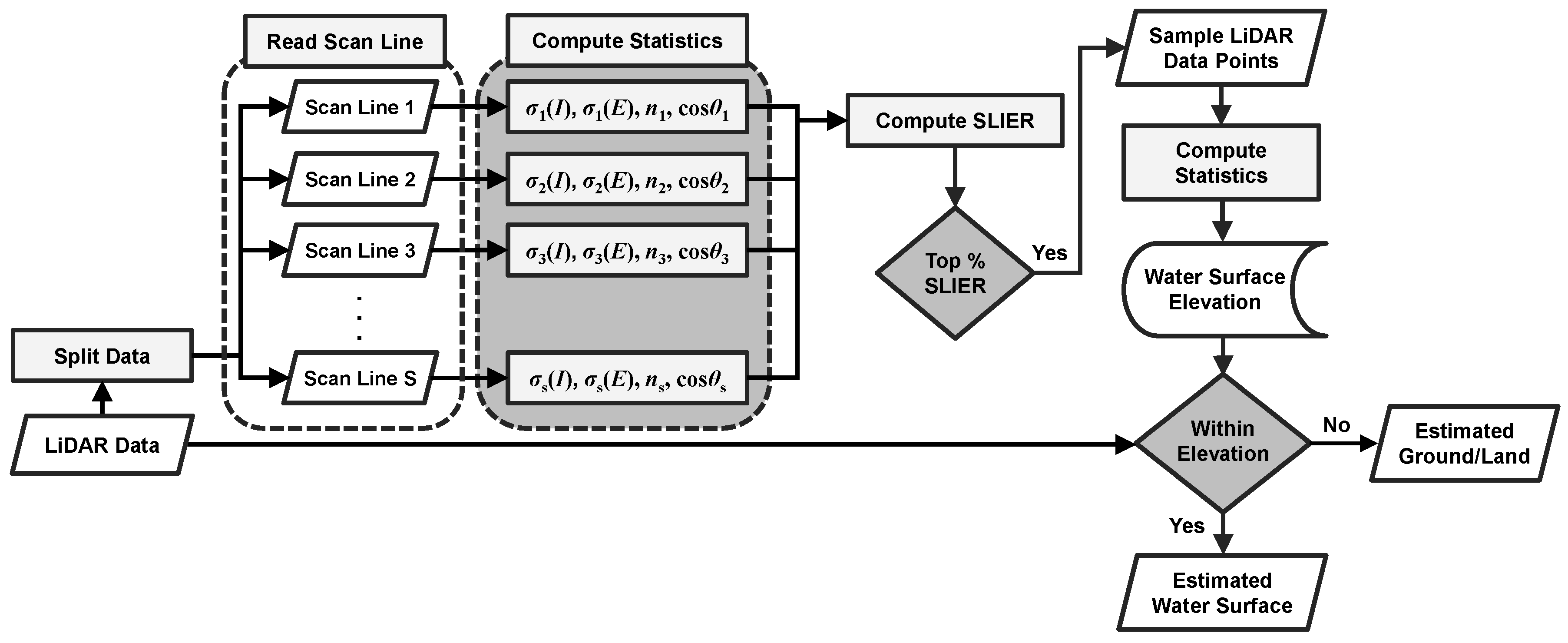
In practice, the workflow of the SLIER computation and its use to extract the water surface can be summarized with the following steps. The process begins by first reading the coordinates, intensity (I), scan angle () and scan direction flag from the LAS data files [32]. Through using the scan direction flag, the LiDAR dataset can be separated in terms of individual scan line (i.e., the scan direction flag with a value of zero refers to a positive scan direction, and vice versa). Subsequently, the SLIER is computed either using Equation (2) or (3) by dividing the standard deviation of intensity by the standard deviation of elevation along each scan line. Once the SLIER is determined for each scan line, those extreme peak values of intensity backscattered from the water surface close to the nadir, which are being treated as outliers, can be located and corrected through computing the MD. Samples of water surface points are identified if they have high SLIER values. Finally, the water surface of the study scene can be estimated through computing the mean and standard deviation of the elevation of the sample water surface points [31].
Figure 4 summarizes the workflow of the SLIER computation and extraction of water bodies. The SLIER can be treated as an automatic training data selection method for mapping water bodies, since most of the existing work relies on either using historical coastline/tidal data or on manual intervention for selecting data training points [33,34,35,36]. With the extracted data points representing the water surface, a machine learning classifier can be trained using these data points in order to delineate the land and water regions, where details can be found in Shaker et al. [37]. One should bear in mind that there are certain assumptions when SLIER is being utilized. Firstly, SLIER can be used for water surface extraction if and only if the swath width (or field of view (FOV)) of the airborne LiDAR data entirely covers the water surface (as illustrated in Figure 2). Secondly, SLIER is mainly designed for linear mode airborne LiDAR sensors operated with an oscillating/rotating mirror or prism. Lastly, SLIER is mostly designed for open water bodies, such as the coastal environment. SLIER is not suitable for a waterfall environment, where the elevation changes through the dataset. Rivers and small streams can be detected if the first criterion is matched and also if sufficient LiDAR data points are collected.
3. Experimental Testing
3.1. Multispectral Airborne LiDAR Dataset
We utilized a multispectral airborne LiDAR dataset collected by Optech Titan for experimental testing and evaluation of the SLIER. The Optech Titan is equipped with three laser channels, where Channel 2 (1064 nm) points at nadir and Channel 1 (1550 nm) and Channel 3 (532 nm) are tilted in the forward direction with 3.5° and 7° off nadir, respectively. Table 1 summarizes the configuration of the multispectral airborne dataset. Most previous research has investigated areas with substantial height differences for man-made shore regions [31,38]; therefore, we intentionally acquired a multispectral LiDAR dataset that mostly covers a natural shore water environment. This dataset is an open dataset found available under the ISPRS Commission 3 website with courtesy of Teledyne Optech [39]. Eight multispectral airborne LiDAR data strips were collected by Optech Titan covering a natural rocky shore area located in Tobermory, Ontario, Canada. The survey was accomplished during July 2015 with a flying height of approximately 500 m and a flying speed 140 kn. With a scan angle of ±20°, the survey extent covers an area of approximately 26.82 km2. Since a relatively high PRF was used (roughly 625 kHz), a high density of data was collected during the flight mission. The total number of data points collected was 787 million, leading to a mean point density of 8.97–11.38 points/m2 and a mean point spacing of approximately 0.3 m. Figure 5 shows the multispectral airborne LiDAR dataset colourized based on the elevation.
3.2. Separability Analysis
Since the dataset included eight data strips with each having three laser channels, a total of 24 LAS files were processed to compute the SLIER, as well as correct the extreme peak intensities backscattered from the water surface. To justify the use of SLIER to provide a good estimate of water surface over the ground, we employed two separability analyses, i.e., transformed divergence (TD) and Bhattacharyya distance (BD), to assess the data separability of land and water. We intentionally compared the results of SLIER, NDWIs derived from original LiDAR intensity and NDWIs derived from the corrected intensity (after being identified by Equation (4)) so as to demonstrate the merit of using SLIER over NDWIs for water surface extraction. The equation of TD can be computed as below:
where:
where refers to the trace of the matrix, i.e., the sum of the diagonal element within the derived matrix. and refer to the variance-covariance matrix of class i and j, respectively, and and refer to the mean vector of class i and j, respectively. As a result, the separability between the land and water sample data points were used to compute the TD and BD based on their values of SLIER and NDWIs. Similarly, BD can be computed as follows:
where:
Regardless of the TD or BD, the computed values are normalized from 0–2 based on Equations (5) and (7). As a rule of thumb, the TD or BD values ranging from 1.9–2.0 imply a good separability between the pair of classes. Values between one and 1.9 refer to poor separability, and values less than one imply that the stated spectral/ratio index cannot provide a good separation between the two classes, where a high mixture of the stated index value exists between the two classes [40].
3.3. Land-Water Classification
After computing the SLIER for each scan line for the three laser channels, the LiDAR data points with “high” SLIER values were treated as water data points. The elevation of these sample water data points was computed, where the instantaneous water surface was estimated with the respective mean and standard deviation of the sample water data points [37]. The estimated water surface points were used to train a statistical classifier, i.e., likelihood model, to perform land-water classification. The likelihood model is listed as:
where refers to the class i, refers to the feature set mean vector of class and refers to the feature set variance-covariance matrix of . and can be created by obtaining all the data points of water/land with features, including elevation, intensity, elevation variation, intensity variation and NDWIs (if multispectral LiDAR data are available). Details of the classification feature sets can be found in Shaker et al. [37]. Finally, for all data points l in L, the data point l is assigned to class , if the computed probability is greater than that of , i.e.,
Since there is a lack of field survey or existing archived coastline for the land-water boundary, the classified point clouds were checked against the reference land and water polygons that were manually digitized with reference to the aerial photos and the LiDAR data. Accuracy assessment was performed by computing the kappa statistics, overall accuracy (OA) and the respective producer’s accuracy (PA) and user’s accuracy (UA) for the land and water class. Various rounds of experimental tests were conducted in order to compare the difference of using monochromatic LiDAR and multispectral LiDAR data for land-water classification.
4. Results and Analysis
4.1. Analysis of the Scan Line Profile
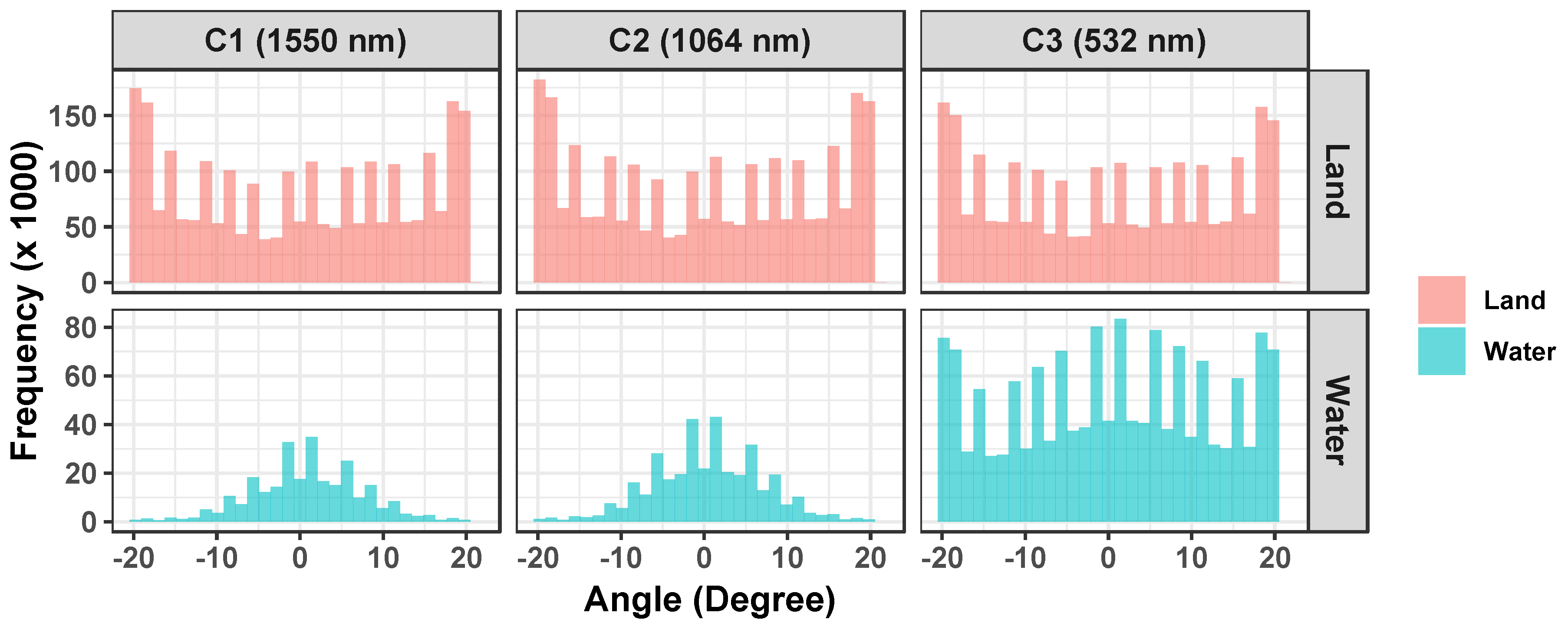
To justify how the three laser channels interact differently between the land and water bodies, we intentionally selected two subsets from one data strip with an area approximately 380 m by 380 m in each to assess the number of data returns. The rationale of selecting 380 m as a sample size is mainly due to the swath width, where data points between the two swath edges can be analysed. The sample data points within these two subsets having either purely land or water are plotted as a data histogram in Figure 6 with respect to the scan angle for the three LiDAR data channels.
As shown in the upper row of Figure 6, the data histograms of land had a similar pattern among the three data channels, where the data points were evenly distributed, except a higher number of data returns being found at both ends of the scan. This can be explained by the mechanism of the oscillating mirror, where the speed of the mirror decelerates at the edges of the scan. Once the mirror stops and changes the scanning direction, the oscillating mirror accelerates to carry on the laser scanning in the opposite direction. Since the PRF remains unchanged during this process, a larger number of data returns can be found at the swath edge due to this speed change [41].
Regarding the water bodies, the histogram of the data returns of the IR and NIR laser channels (i.e., Channels 1 and 2) both had a higher number of data returns at the close to the nadir region and a lesser number of data returns at large scan angles. The fewer number of data points at large incidence angles can be explained by the effect of laser dropouts [26]. The difference of the number of data returns between the nadir and the swath edge was up to 97% in these two histograms. As a result, the histogram pattern appeared similar to a normal distribution. Regarding the histograms of the green data channel (Channel 3), the data return pattern on the water bodies was similar to those collected from the ground. Based on this observation, one can note that the water bodies had a fewer number of data points at the swath edge (i.e., large incidence angles), leading to a fewer number of data points for each scan line in Channels 1 (1550 nm) and 2 (1064 nm). This justifies the use of the number of data points () and the cosine of the scan angle () in Equation (3) to derive SLIER, so as to make the water bodies discriminated from the land.
To describe statistically the difference among the data histograms, we employed the Kolmogorov–Smirnov (KS) test to measure the similarity between a pair of histograms [42]. The KS test aims to compute the cumulative distribution function of any two histograms and to look for the largest difference between the two distribution functions (named D-statistic). Table 2 shows the computed D-statistic of the KS test between a pair of data histograms from the three data channels. With all the computed D-statistic, we compared these values with their respective critical value with, say, the 99.9% confidence interval (i.e., p = 0.001). Based on the statistical analysis, it was found that only the D-statistic between histograms of C1 (water) and C2 (water) was less than or equal to the critical value (i.e., 0.0017), where the rest of the D-statistic values were larger than their respective critical value. Despite that, some of the D-statistic values were small and close to the critical value, including C1 (land) vs. C2 (land), C1 (water) vs. C3 (water) and C2 (water) vs. C3 (water). By running the KS test, we concluded that the histograms of C1 (water) and C2 (water) were similar, whereas the rest of the histograms were slightly or significantly different from each other.
4.2. Separability Analysis
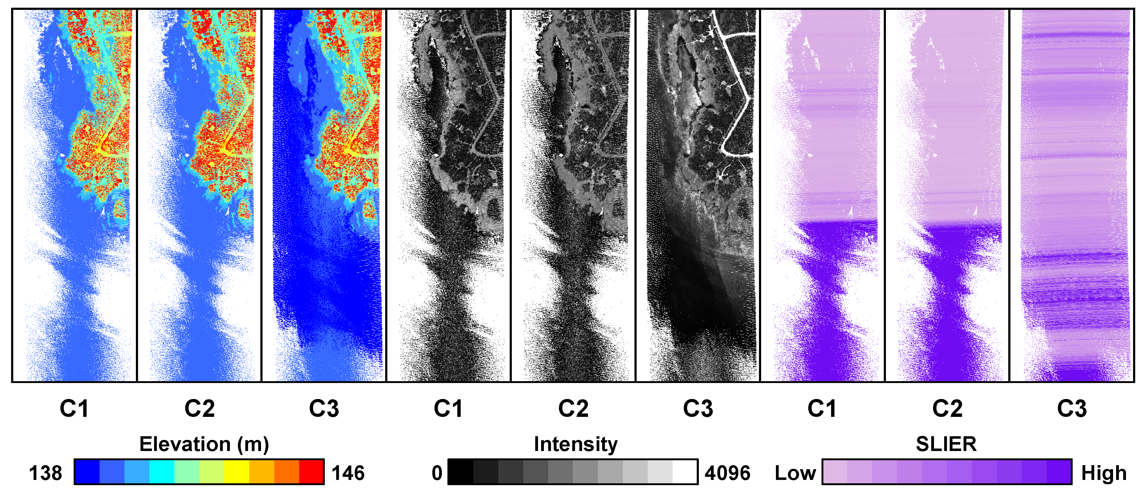
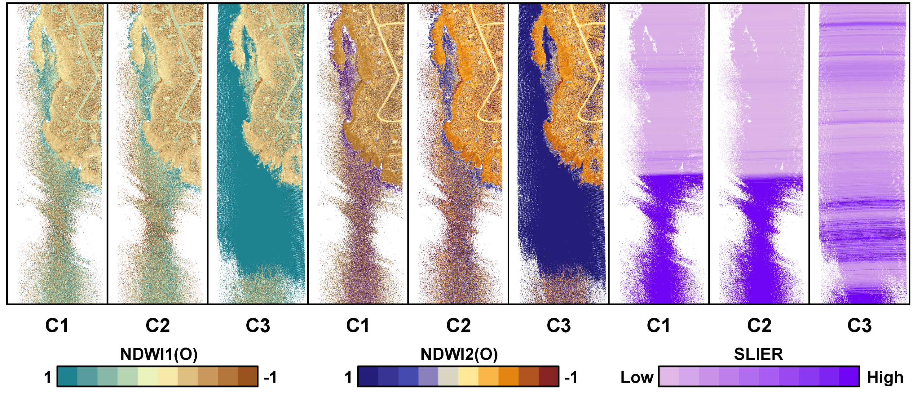
Figure 7 shows a shore region of the multispectral LiDAR data displayed in individual channels together with the derived SLIER. Based on the displayed figures, one can easily note that the laser dropouts appeared significantly in the water region at large scan angles, particularly in Channels 1 and 2, resulting in a large portion of missing data found at the swath edge. Since the green channel is capable of collecting both the water surface and the bottom, the effect of laser dropouts was not obvious in Channel 3. Regarding the intensity value, extreme peak intensity values were found close to the nadir region, regardless of the laser channel. All these properties resulted in high SLIER values being computed in Channels 1 and 2 on the water region, whereas this effect was not obvious in the SLIER computed using Channel 3.
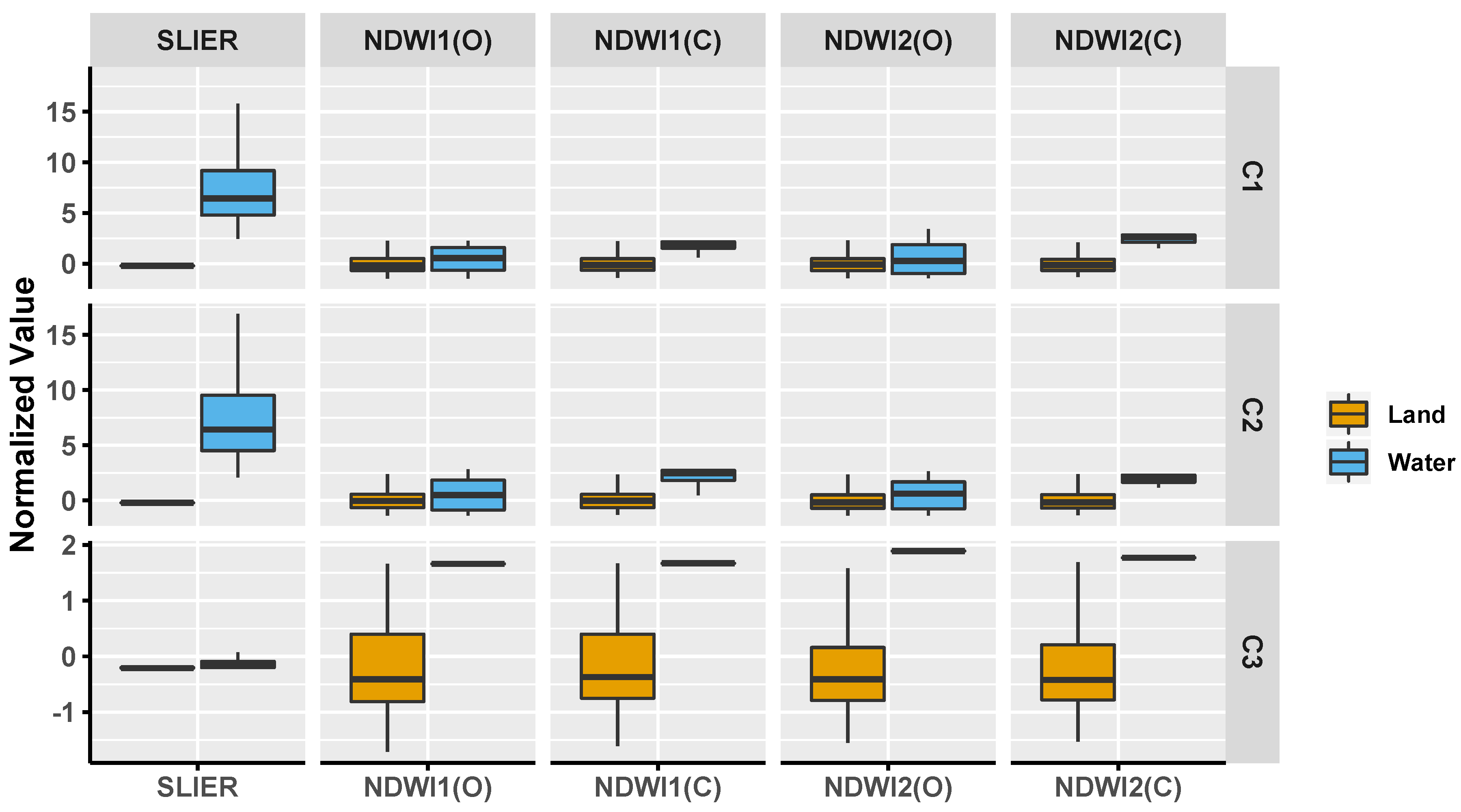
Since multispectral airborne LiDAR datasets were acquired in this study, two NDWIs could be derived based on Equation (1). NDWI1 here refers to the NDWI derived by using the intensity of Channel 3 (532 nm) as and the intensity of Channel 2 (1064 nm) as . On the other hand, NDWI2 was derived using the intensity of Channel 3 (532 nm) as and the intensity of Channel 1 (1550 nm) as . Since the values of SLIER and NDWIs are unitless, it is not scientifically sound to compare their absolute values. Therefore, the values of SLIER and NDWIs were first normalized using their respective mean and standard deviation based on the z-score. Afterwards, the boxplots of land and water data samples were generated based on SLIER, the two NDWIs derived using the corrected intensity data (as reported in Equation (4)) and the two NDWIs derived using the original intensity data (see Figure 8), where the box represents the interquartile range (IQR) of the data (i.e., 25th–75th percentiles). One should note that the corresponding row shown in Figure 8 refers to the selection of the core channel. For instance, the first row indicates that C1 is the core channel, where the intensity values of the nearest C2’s and C3’s points are assigned to C1 in order to compute the NDWIs.
One can easily observe that the use of SLIER, particularly derived by Channels 1 and 2, offered a high separability between land and water, since their corresponding boxplots do not have any overlap. The normalized values of SLIER in Channels 1 and 2 were significantly greater than zero, where their median value was close to six. Contradictorily, SLIER derived using Channel 3 did not appear in the same manner as Channels 1 and 2. This can be ascribed by the computation of SLIER through reading the individual scan line, where both water surface and bottom returns are included in each scan line. As a result, a high variation of elevation along each scan line cannot yield a high value of SLIER for water bodies. Regardless of the laser channel, SLIER still outperformed NDWIs in terms of separating land and water regions. When using original intensity data to derive NDWI (i.e., NDWI(O)), both NDWI1(O) and NDWI2(O) were observed with a high mixture of values between land and water regions in Channels 1 and 2 (i.e., their corresponding boxplots had large overlap). However, the corrected intensity was able to reduce the variance of water bodies, where there existed a good separation between the boxplots of land and water, leading to a reduction of variance of NDWI1(C) and NDWI2(C) in these two channels. In Channel 3, a high variance of NDWIs was found on land, whereas the NDWIs of water bodies were well above the land values, whether the original or corrected intensity data were used. Figure 9 shows the results of NDWI1(O) and NDWI2(O).
To describe the separability statistically, we employed the BD and TD measures as mentioned in Section 3.2. Table 3 shows the results of BD and TD computed using the land and water data points. Only the SLIER derived by Channels 1 and 2 offered a high separability in terms of TD and BD, where their respective values were consistently greater than 1.9. Although the TD measure of SLIER, NDWI1(C) and NDWI2(C) was above 1.9 in Channel 3, their corresponding BD value ranged only from 1.1–1.5, offering a mild separability. The rest of the other values, particularly those NDWIs derived using original intensity data, were mostly below one. The TD and BD of NDWI1(O) and NDWI2(O) were even less than 0.2 in Channels 1 and 2. However, removal of those extreme peak intensities on water surface can result in an improvement of separability between land and water, where their respective TD and BD values were improved up to 0.5 and 0.8. Therefore, our experimental comparison proved that SLIER outperformed the traditional NDWIs, particularly in Channels 1 and 2, in terms of providing a good separability between land and water regions.
4.3. Determination of the SLIER Threshold for Water Surface Extraction
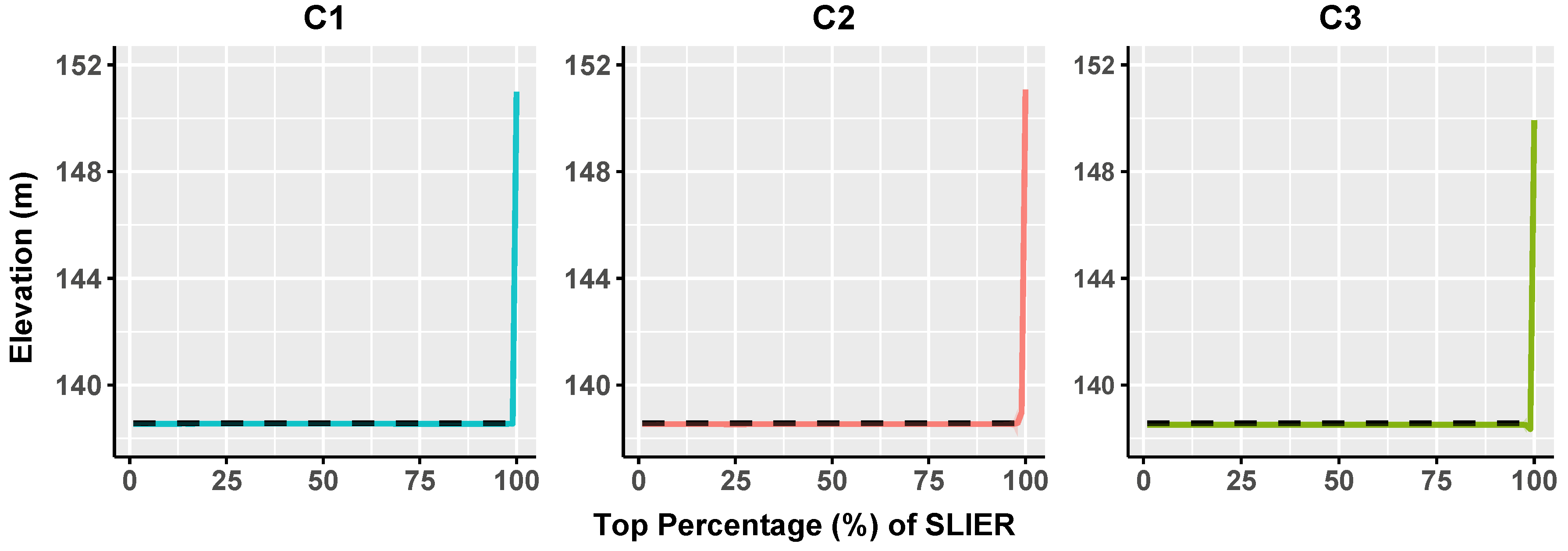
Based on the above-mentioned analyses, it is proven that SLIER is able to provide a good separability between land and water regions. Unlike traditional NDWIs where a threshold of zero can be used as a cut-off value for extracting certain water bodies, we should analyse the strategy of how “large” the SLIER value should be in order to identify the data sample points and determine the water surface region. As a result, we plot Figure 10, which shows the top “X” percentage of SLIER with respect to the extracted data sample points’ elevation for the three LiDAR data channels. The dotted grey line represents the instantaneous water surface elevation computed based on the identifying water region from the aerial photos.
It is obvious that the elevation of the extracted data points based on the top 1–97% of the SLIER value was very close to the instantaneous water surface (∼138.56 m), where the elevation of the extracted data points were 138.55 ± 0.05 m, 138.53 ± 0.07 m and 138.51 ± 0.04 m for Channels 1–3, respectively. Since there was no significant difference between the top 1–97% of the SLIER value for extracting the data sample points, we identified the top 10% of the SLIER value as a recommended setting for the subsequent experiments. Once the water surface was estimated, all the data points below this surface (mean elevation plus two S.D.) were treated as training data for water bodies, whereas all the data points above such an elevation were regarded as training data for land. One should bear in mind that such a strategy of water surface estimation can be modified if a land depression is found in the near shore region; details are reported in Shaker et al. [37].
4.4. Land-Water Classification
Finally, the SLIER-derived training datasets were utilized to train the maximum likelihood model, as reported in Section 3.3, to conduct the land-water classification. Various feature sets were created to train the likelihood model, including the elevation (E), three intensity data (), intensity variation (), elevation variation () and number of returns (N). The intensity value here refers to the corrected intensity after removing the extreme peak intensity through Equation (4). Since multispectral LiDAR data were available in our experiment, three normalized difference feature indices (NDFIs) (i.e., NDWI1, NDWI2 and the other one derived using 1064 nm and 1550 nm) were also incorporated as feature sets to improve the classification capability [37]. A core channel was first selected, and the intensity values from the other two channels were assigned to the core channel. As a result, three rounds of experiments were conducted for the land-water classification with each of the three channels being selected as the core channel together with ten feature sets (, NDFI1, NDFI2 and NDFI3). One should note that the NDFI3 refers to the ratio index computed based on the NIR and IR channel. To demonstrate the merit of having multispectral LiDAR intensity data, we also conducted the land-water classification using monochromatic LiDAR feature sets (i.e., ), which all can be derived based on any single laser channel.
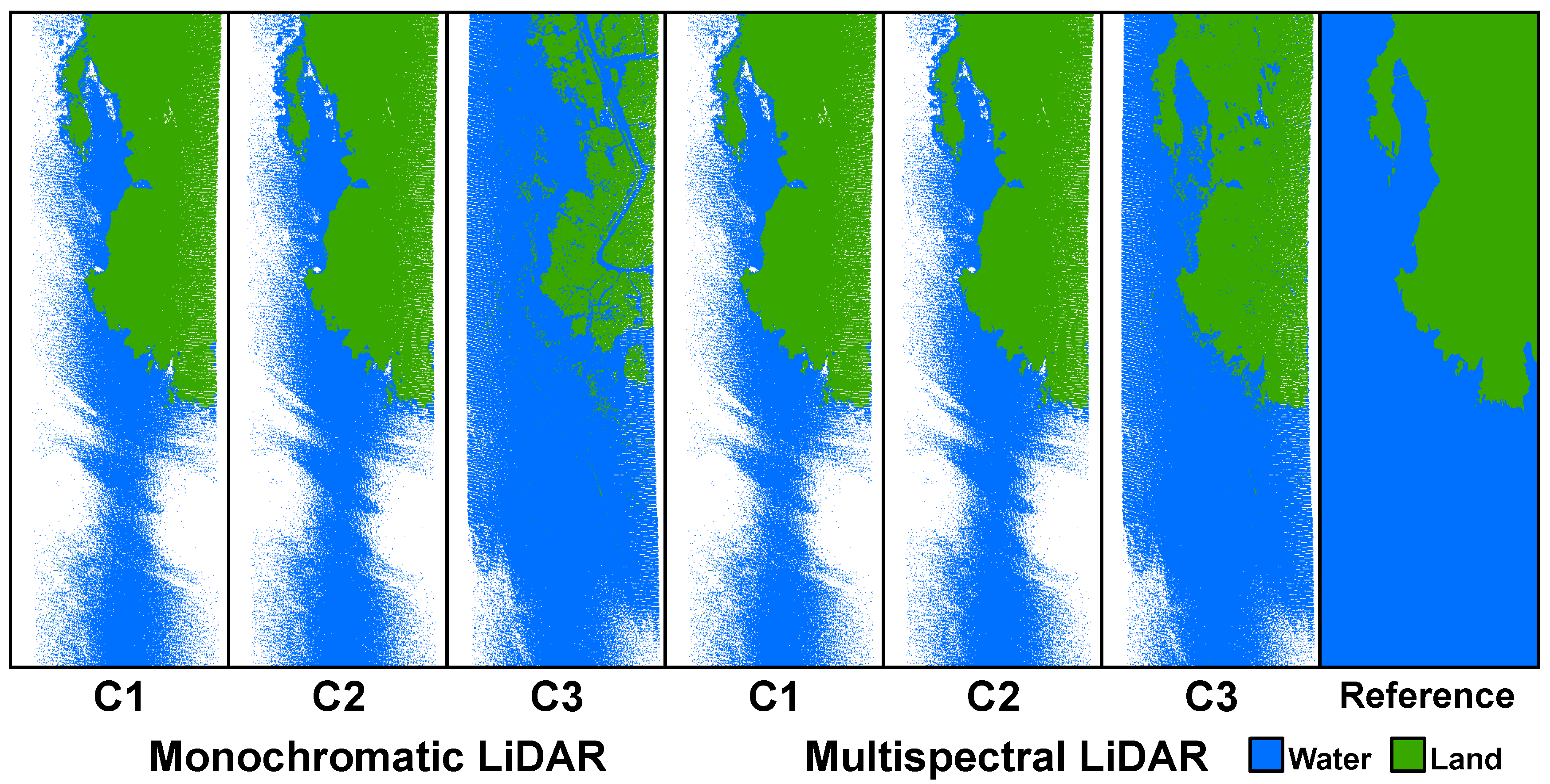
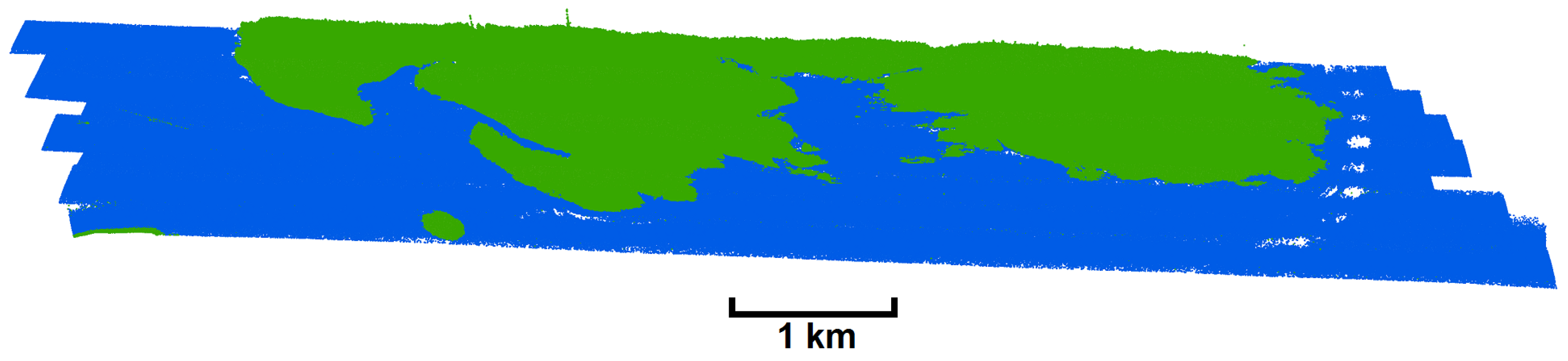
The overall accuracy was derived based on comparing the classification results with the digitized land-water boundary with reference to the aerial photos and the LiDAR data. Table 4 summarizes the OA, UA, PA and kappa statistics of the experimental trials for land-water classification. Figure 11 shows the classification results using monochromatic or multispectral LiDAR data. The OA of land-water classification using either Channel 1 or 2 as a core channel was 99.14% and 99.15%, respectively, using the monochromatic LiDAR data (five feature sets). A slight improvement of OA by 0.1–0.2% was achieved while using the multispectral LiDAR data (ten feature sets). Indeed, the accuracy of water mapping was over 99.5% (i.e., PA of water) in both cases, whereas the accuracy of land mapping was slightly less than that of water (∼97–98%). The use of Channel 3 as a core channel for classification produced a slightly lower accuracy, for which the OA was close to 94.3% in the case of using five feature sets. As shown in Figure 11, the water surface estimated by SLIER seemed to be higher than its actual elevation, resulting in the near shore land region being misclassified as water. However, if multispectral LiDAR intensity and NDWIs were used, the classification result was improved by 4%, resulting in an OA of 98.36%. The water mapping accuracy was around 99% when using five or ten feature sets. Nevertheless, the land mapping accuracy was significantly improved from 89.23–97.40% when the multispectral LiDAR dataset was used. The relatively lower accuracy in Channel 3 can be attributed to the multiple returns from the water surface and bottom, which caused the elevation estimated by the “high” SLIER value having a higher standard deviation. That would subsequently lead to a less accurate water surface being estimated. In addition, the recorded intensities of Channels 1 and 2 both had a high reflectance value for the rocky shore. It thus helped Channels 1 and 2 (both NIR and IR lasers) to produce a better accuracy than that of Channel 3 for the land-water classification. Such a phenomenon can also be justified by the spectral reflectance profile shown in Figure 1. Figure 12 shows the multispectral LiDAR data classification result using Channel 1 as the core channel.
4.5. Additional Experiment on Monochromatic LiDAR Data
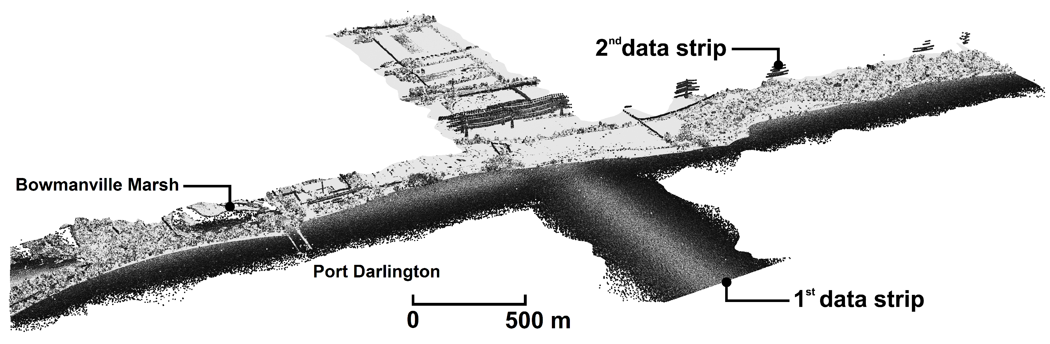
The above experiment successfully demonstrated that SLIER is capable of removing the extreme intensity values on the water surface and improving the separability between land and water regions. All these can subsequently lead to an accurate land-water classification using multispectral airborne LiDAR data. To prove the same capability of SLIER toward monochromatic airborne LiDAR data, additional experiments were carried out using a single-wavelength (1064 nm) LiDAR dataset collected by an Optech Galaxy on a near-shore region of Lake Ontario, Bowmanville, Ontario, Canada. The data were acquired on 30 May 2018, where the system settings of Galaxy were: PRF = 350 kHz, SF = 40 Hz, SA = ±30° and flying altitude ≈600 m. We intentionally examined two data strips collected in different directions, where the first data strip was collected perpendicular to the shore while the second strip was acquired parallel to the shore. The following Figure 13 shows the LiDAR intensity data of the two data strips.
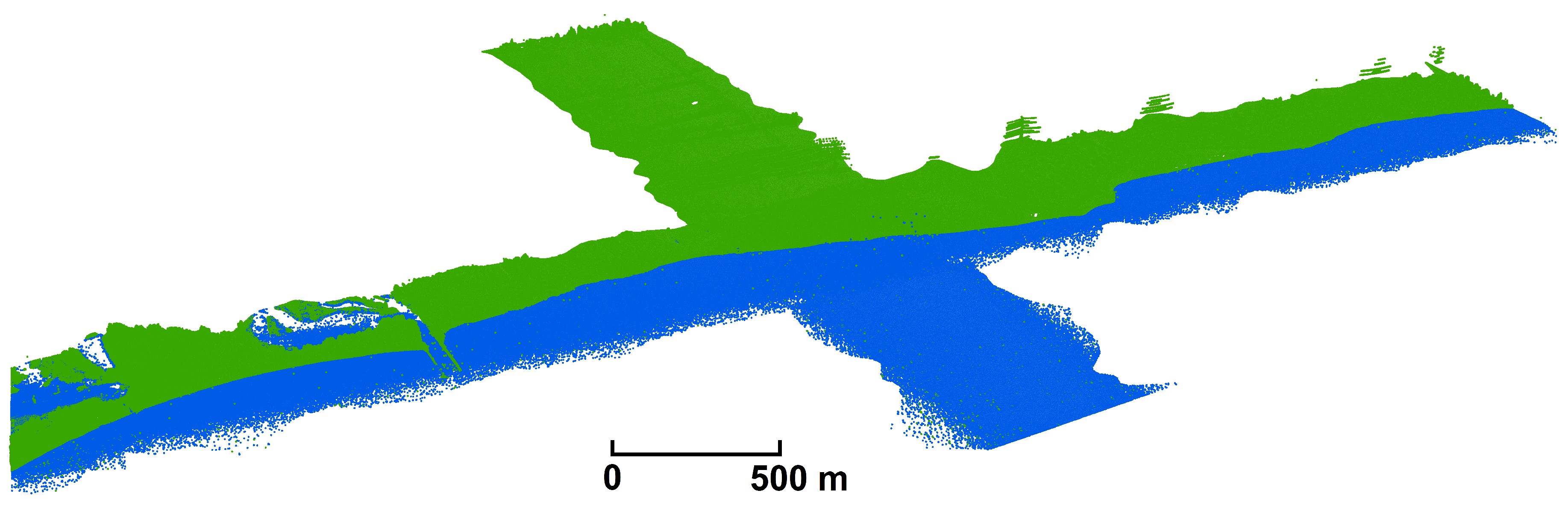
Since the first data strip had a full FOV covering the water region, SLIER was first implemented on this data strip in order to estimate the elevation of the water surface (mean and standard deviation) by extracting those data points with the top 10% of the SLIER value. As the second data strip did not have a full coverage of the water region in any part of the data, SLIER should not be used under this circumstance. Thus, the estimated statistics of water surface from the first data strip were then transferred to the second data strip for training data selection. Following the land-water classification workflow as previously proposed in [37], feature sets including I, E, , and N were used to train a likelihood model to perform the land-water classification. Figure 14 shows the land-water classification result using the Optech Galaxy dataset. Accuracy assessment was conducted with reference to a set of land and water polygons digitized based on the aerial photos and the LiDAR data.
The computed OA based on the reference data yielded 99.27% in this case study, which is similar to the aforementioned case study. The PA of land and water was 99.54% and 98.42%, respectively, whereas the UA of land and water was 99.51% and 98.53%, respectively. The classification result successfully identified the shore boundary and preserved those near-shore features, such as the two rocky piers near Port Darlington, Ontario, Canada. One can note that the misclassified points can be attributed to the appearance of aquatic vegetation and wetland found on the Bowmanville Marsh. Since the study area has an obvious elevation difference between the land and water regions, a monochromatic airborne LiDAR dataset is mostly capable of producing a high accuracy in land-water classification.
4.6. Discussion
Based on the above analyses, our experiment successfully demonstrated SLIER to be a reliable ratio index that is able to provide a high separability between the land and water regions for both monochromatic and multispectral airborne LiDAR data. Unlike traditional passive remote sensing data that require different spectral bands to derive the water index, SLIER can be implemented on either monochromatic or multispectral airborne LiDAR data. As long as some of the airborne LiDAR data scan lines are completely collected over the water region, the computed SLIER reaps the benefit of the high variation of intensity backscattered from a relatively flat water surface, and thus provides a high separability between the water and ground. SLIER does not have any restriction toward the flight direction, where the LiDAR scan can be either conducted parallel or perpendicular to the open water environment. In addition, SLIER can be applied to the inland river environment, as long as the river region is completely covered by some of the scan lines that have sufficient data returns. However, SLIER may not be suitable for waterfalls or rivers with significant changes of elevation. If the elevation difference found on the ground is close to the elevation difference found on the water region, the denominator of SLIER (i.e., standard deviation of elevation along each scan line) cannot give a boost to further distinguish these two classes. One should bear in mind that SLIER is suitable only for those airborne LiDAR data collected by sensors operated with a rotating prism or oscillating mirror, resulting in a scan line pattern. Since the green laser signal is capable of collecting returns from both the water surface and bottom, the NIR/IR lasers operated with wavelengths 1064 nm and 1550 nm are deemed to be appropriate for SLIER due to their unique return of the water surface.
The significance of SLIER’s development can be justified in various ways. Some of the existing approaches of land-water classification using airborne LiDAR data require supplementary information, such as historical coastline [35], tidal data [36] or manual intervention to define the training data [33,34]. Furthermore, for a classification approach such as the use of the Gaussian mixture model to split preliminarily the elevation histogram for estimating land and water [37], users are required to define manually or utilize model selection methods (such as the Akaike information criterion or Bayesian information criterion) to input the number of components. SLIER can remove the necessity of prior information or manual intervention in order to provide a robust estimation of the water surface, which leads to an accurate land-water classification. Finally, based on our experimental tests, SLIER outperforms traditional NDWIs in terms of providing a high separability between the land and water regions, particularly for the SLIER derived by Channel 1 (1550 nm) and channel 2 (1064 nm). Furthermore, the water surface extracted by SLIER can aid in generating the hydro-flattened digital elevation model. As a result, SLIER does not require any selection of parameters, training samples or iteration, and thus gives this approach a high degree of automation and significant practical relevance.
5. Conclusions
An airborne LiDAR-based ratio index, named SLIER, was proposed for serving the purpose of automatic extraction of the water surface from airborne LiDAR 3D data point cloud. SLIER maximizes the benefits of using both the geometric and radiometric components of airborne LiDAR data, and it is mainly computed by dividing the standard deviation of intensity over the standard deviation of elevation along each scan line. As attributed to the uniqueness of how the laser interacts with the water bodies, higher SLIER values are always found on the water bodies compared to the land. As a result, the instantaneous water surface can be estimated through extracting those LiDAR data points with high SLIER values and subsequently computing their mean elevation. The estimated water surface can be used as training data to serve the subsequent land-water classification. Based on our experiments of SLIER on monochromatic and multispectral airborne LiDAR datasets, the following conclusions are drawn.
- Since the NIR/IR laser (1064 nm or 1550 nm) is usually backscattered from the water surface, the implementation of SLIER on NIR/IR laser data has a better estimation of the water surface than that derived from the green laser data (532 nm), where multiple returns are found on the water surface and column.
- Unlike a traditional spectral water index derived from optical remote sensing image, SLIER can be computed using either monochromatic or multispectral airborne LiDAR data and is not affected by the presence of shadow or other low albedo dark features. In addition, SLIER outperforms the traditional NDWIs in terms of providing high separability between the land and water regions, regardless of the laser channel.
- Extreme peaks of intensity found on the water surface can be identified and removed by computing the Mahalanobis distance using the original intensity and SLIER values.
- With the water surface being extracted from the LiDAR data points having “high” SLIER values (the top 10% is recommended), the estimated water surface can be used to train a machine learning model for land-water classification.
- A land-water classification accuracy of over 98% was achieved using the SLIER-derived training data, regardless of the laser channel being used. In particular, Channels 1 (1550 nm) and 2 (1064 nm) produced over 99% of land-water classification accuracy and water mapping accuracy, whether using monochromatic LiDAR or multispectral LiDAR feature sets. When Channel 3 was used as the core channel, the overall accuracy was only 94.3%, and the overall accuracy was improved up to 98.36% when multispectral LiDAR intensity and NDWIs were incorporated for classification.
To implement SLIER for estimating the water surface, one should bear in mind the following requirements during data collection. Firstly, the study area should be surveyed by a linear mode airborne LiDAR system operated with an oscillating mirror or a rotating prism, resulting in a scan line pattern. SLIER may not work well if it is directly implemented on those data collected by conical scanning systems (such as CZMIL or Chiroptera). Furthermore, the airborne LiDAR survey should cover both land and water regions. However, the flight mission should be planned and configured so that some of the scan lines completely cover the water region. Lastly, SLIER is mainly designed for mapping a water surface that does not have a significant change of elevation, including any near-shore, open water or inland delta environment. Waterfalls, rivers with dramatic elevation changes or shore regions with high tidal waves may not be appropriate. It is hoped that SLIER can be widely adopted by the airborne LiDAR community as a robust water ratio index, similar to the NDWIs being universally used in the optical remote sensing images.
Author Contributions
Conceptualization, W.Y.Y. and A.S.; data curation, P.E.L.; validation, W.Y.Y., A.S.; formal analysis, W.Y.Y.; investigation, W.Y.Y.; methodology, W.Y.Y.; supervision, A.S.; writing, original draft, W.Y.Y.; writing, review and editing, W.Y.Y., A.S. and P.E.L.
Funding
This study is financially supported by the Natural Sciences and Engineering Research Council of Canada (NSERC) Collaborative Research and Development (CRD) Grant.
Acknowledgments
The authors would like to express their appreciation to the following individuals who brought in many illuminating discussions during the study: Joe Liadsky (former Chief Technology Officer), Alex Yeryomin, Michael Sitar and Ana Paula Kersting.
Conflicts of Interest
The airborne LiDAR data used in the experiments were collected by Teledyne Optech’s airborne surveying team.
Abbreviations
The following abbreviations are used in this manuscript:
| BD | Bhattacharyya distance |
| FOV | Field of view |
| IR | Infrared |
| LiDAR | Light Detection and Ranging |
| MD | Mahalanobis distance |
| NDWI | Normalized difference water index |
| NIR | Near-infrared |
| OA | Overall accuracy |
| PA | Producer’s accuracy |
| SLIER | Scan line intensity-elevation ratio |
| TD | Transformed divergence |
| UA | User’s accuracy |
References
- McFeeters, S.K. The use of the Normalized Difference Water Index (NDWI) in the delineation of open water features. Int. J. Remote Sens. 1996, 17, 1425–1432. [Google Scholar] [CrossRef]
- Gao, B.C. NDWI—A normalized difference water index for remote sensing of vegetation liquid water from space. Remote Sens. Environ. 1996, 58, 257–266. [Google Scholar] [CrossRef]
- Vrieling, A. Satellite remote sensing for water erosion assessment: A review. Catena 2006, 65, 2–18. [Google Scholar] [CrossRef]
- Smith, L.C. Satellite remote sensing of river inundation area, stage, and discharge: A review. Hydrol. Process. 1997, 11, 1427–1439. [Google Scholar] [CrossRef]
- Matthews, M.W. A current review of empirical procedures of remote sensing in inland and near-coastal transitional waters. Int. J. Remote Sens. 2011, 32, 6855–6899. [Google Scholar] [CrossRef]
- Gordon, H.R.; Morel, A.Y. Remote Assessment of Ocean Color for Interpretation of Satellite Visible Imagery: A Review; Springer Science & Business Media: New York, NY, USA, 2012; Volume 4. [Google Scholar]
- Baldridge, A.; Hook, S.; Grove, C.; Rivera, G. The ASTER spectral library version 2.0. Remote Sens. Environ. 2009, 113, 711–715. [Google Scholar] [CrossRef]
- Palmer, S.C.; Kutser, T.; Hunter, P.D. Remote sensing of inland waters: Challenges, progress and future directions. Remote Sens. Environ. 2015, 5157, 1–8. [Google Scholar] [CrossRef]
- Yan, W.Y.; Shaker, A.; El-Ashmawy, N. Urban land cover classification using airborne LiDAR data: A review. Remote Sens. Environ. 2015, 158, 295–310. [Google Scholar]
- Kay, S.; Hedley, J.; Lavender, S. Sun glint correction of high and low spatial resolution images of aquatic scenes: A review of methods for visible and near-infrared wavelengths. Remote Sens. 2009, 1, 697–730. [Google Scholar] [CrossRef]
- Mandlburger, G. A Case Study on Through-Water Dense Image Matching. Int. Arch. Photogramm. Remote Sens. Spat. Inf. Sci. 2018, 42, 659–666. [Google Scholar] [CrossRef]
- Meesuk, V.; Vojinovic, Z.; Mynett, A.E.; Abdullah, A.F. Urban flood modelling combining top-view LiDAR data with ground-view SfM observations. Adv. Water Resour. 2015, 75, 105–117. [Google Scholar] [CrossRef]
- Hunt, K.; Royall, D. A LiDAR-based analysis of stream channel cross section change across an urban–rural land-use boundary. Prof. Geogr. 2013, 65, 296–311. [Google Scholar] [CrossRef]
- Lane, C.R.; D’Amico, E. Calculating the ecosystem service of water storage in isolated wetlands using LiDAR in north central Florida, USA. Wetlands 2010, 30, 967–977. [Google Scholar] [CrossRef]
- Irish, J.; White, T. Coastal engineering applications of high-resolution lidar bathymetry. Coast. Eng. 1998, 35, 47–71. [Google Scholar] [CrossRef]
- Brock, J.C.; Wright, C.W.; Sallenger, A.H.; Krabill, W.B.; Swift, R.N. Basis and methods of NASA airborne topographic mapper lidar surveys for coastal studies. J. Coast. Res. 2002, 18, 1–13. [Google Scholar]
- Guenther, G.C.; Cunningham, A.G.; LaRocque, P.E.; Reid, D.J. Meeting the accuracy challenge in airborne LiDAR bathymetry. In Proceedings of the EARSeL-SIG-Workshop LiDAR, Dresden, Germany, 16–17 June 2000; pp. 1–27. [Google Scholar]
- Allouis, T.; Bailly, J.S.; Pastol, Y.; Le Roux, C. Comparison of LiDAR waveform processing methods for very shallow water bathymetry using Raman, near-infrared and green signals. Earth Surf. Process. Landf. 2010, 35, 640–650. [Google Scholar] [CrossRef]
- Guenther, G.C.; Thomas, R.W.; LaRocque, P.E. Design considerations for achieving high accuracy with the SHOALS bathymetric lidar system. In CIS Selected Papers: Laser Remote Sensing of Natural Waters: From Theory to Practice; International Society for Optics and Photonics: San Diego, CA, USA, 1996; Volume 2964, pp. 54–72. [Google Scholar]
- Guenther, G.C.; Brooks, M.W.; LaRocque, P.E. New capabilities of the “SHOALS” airborne LiDAR bathymeter. Remote Sens. Environ. 2000, 73, 247–255. [Google Scholar] [CrossRef]
- Wang, C.K.; Philpot, W.D. Using airborne bathymetric LiDAR to detect bottom type variation in shallow waters. Remote Sens. Environ. 2007, 106, 123–135. [Google Scholar] [CrossRef]
- Zhao, J.; Zhao, X.; Zhang, H.; Zhou, F. Improved model for depth bias correction in airborne LiDAR bathymetry systems. Remote Sens. 2017, 9, 710. [Google Scholar] [CrossRef]
- Bufton, J.L.; Hoge, F.E.; Swift, R.N. Airborne measurements of laser backscatter from the ocean surface. Appl. Opt. 1983, 22, 2603–2618. [Google Scholar] [CrossRef]
- Pe’Eri, S.; Philpot, W. Increasing the existence of very shallow-water LiDAR measurements using the red-channel waveforms. IEEE Trans. Geosci. Remote Sens. 2007, 45, 1217–1223. [Google Scholar] [CrossRef]
- Li, Z.; Lemmerz, C.; Paffrath, U.; Reitebuch, O.; Witschas, B. Airborne Doppler LiDAR investigation of sea surface reflectance at a 355-nm ultraviolet wavelength. J. Atmos. Ocean. Technol. 2010, 27, 693–704. [Google Scholar] [CrossRef]
- Höfle, B.; Vetter, M.; Pfeifer, N.; Mandlburger, G.; Stötter, J. Water surface mapping from airborne laser scanning using signal intensity and elevation data. Earth Surf. Process. Landf. 2009, 34, 1635–1649. [Google Scholar] [CrossRef]
- Tamari, S.; Mory, J.; Guerrero-Meza, V. Testing a near-infrared LiDAR mounted with a large incidence angle to monitor the water level of turbid reservoirs. ISPRS J. Photogramm. Remote Sens. 2011, 66, S85–S91. [Google Scholar] [CrossRef]
- Vain, A.; Yu, X.; Kaasalainen, S.; Hyyppa, J. Correcting airborne laser scanning intensity data for automatic gain control effect. IEEE Geosci. Remote Sens. Lett. 2010, 7, 511–514. [Google Scholar] [CrossRef]
- Fernandez-Diaz, J.C.; Carter, W.E.; Glennie, C.; Shrestha, R.L.; Pan, Z.; Ekhtari, N.; Singhania, A.; Hauser, D.; Sartori, M. Capability assessment and performance metrics for the Titan multispectral mapping LiDAR. Remote Sens. 2016, 8, 936. [Google Scholar] [CrossRef]
- Stevens, C.W.; Wolfe, S.A. High-resolution mapping of wet terrain within discontinuous permafrost using LiDAR intensity. Permafr. Periglac. Process. 2012, 23, 334–341. [Google Scholar] [CrossRef]
- Yan, W.Y.; Shaker, A.; LaRocque, P.E. Water mapping using multispectral airborne LiDAR ata. Int. Arch. Photogramm. Remote Sens. Spat. Inf. Sci. 2018, XLII-3, 2047–2052. [Google Scholar] [CrossRef]
- The American Society for Photogrammetry & Remote Sensing. LAS Specification, Version 1.4-R13. Available online: https://www.asprs.org/wp-content/uploads/2010/12/LAS_1_4_r13.pdf (accessed on 29 March 2019).
- Brzank, A.; Heipke, C.; Goepfert, J.; Soergel, U. Aspects of generating precise digital terrain models in the Wadden Sea from LiDAR–water classification and structure line extraction. ISPRS J. Photogramm. Remote Sens. 2008, 63, 510–528. [Google Scholar] [CrossRef]
- Yuan, X.; Sarma, V. Automatic urban water-body detection and segmentation from sparse ALSM data via spatially constrained model-driven clustering. IEEE Geosci. Remote Sens. Lett. 2011, 8, 73–77. [Google Scholar] [CrossRef]
- Smeeckaert, J.; Mallet, C.; David, N.; Chehata, N.; Ferraz, A. Large-scale classification of water areas using airborne topographic LiDAR data. Remote Sens. Environ. 2013, 138, 134–148. [Google Scholar] [CrossRef]
- Yousef, A.; Iftekharuddin, K.M.; Karim, M.A. Shoreline extraction from light detection and ranging digital elevation model data and aerial images. Opt. Eng. 2014, 53, 011006. [Google Scholar] [CrossRef]
- Shaker, A.; Yan, W.Y.; LaRocque, P.E. Automatic land-water classification using multispectral airborne LiDAR data for near shore and river environment. ISPRS J. Photogramm. Remote Sens. 2019. submitted. [Google Scholar]
- Morsy, S.; Shaker, A.; El-Rabbany, A. Using multispectral airborne LiDAR data for land/water discrimination: A case study at Lake Ontario, Canada. Appl. Sci. 2018, 8, 349. [Google Scholar] [CrossRef]
- The International Society for Photogrammetry and Remote Sensing. III/5 Announcement for Free Multi-Spectral and Mobile LiDAR Data. Available online: http://www2.isprs.org/commissions/comm3/wg5/news.html (accessed on 29 March 2019).
- Jensen, J.R. Introductory Digital Image Processing: A Remote Sensing Perspective, 3rd ed.; Pearson Prentice Hall: Upper Saddle River, NJ, USA, 2005. [Google Scholar]
- Yan, W.Y.; Shaker, A. Airborne LiDAR intensity banding: Cause and solution. ISPRS J. Photogramm. Remote Sens. 2018, 142, 301–310. [Google Scholar] [CrossRef]
- Kolmogorov, A. Sulla determinazione empirica di una legge di distribuzione. Giornale dell’Istituto Italiano Degli Attuari 1933, 4, 83–91. [Google Scholar]
Figure 1.
Spectral reflectance of different man-made and natural features (Data obtained from the NASA ASTER Spectral Library [7]).
Figure 1.
Spectral reflectance of different man-made and natural features (Data obtained from the NASA ASTER Spectral Library [7]).

Figure 2.
Illustration of the airborne LiDAR data’s scan line profile acquired from land and water. Compared to the land, the water region usually has a high fluctuation of intensity and low variation of elevation along each scan line, and laser dropouts can also be found at large incidence angles.
Figure 2.
Illustration of the airborne LiDAR data’s scan line profile acquired from land and water. Compared to the land, the water region usually has a high fluctuation of intensity and low variation of elevation along each scan line, and laser dropouts can also be found at large incidence angles.

Figure 3.
Examples of LiDAR intensity data having a high fluctuation of intensity values on water bodies (top row = near-infrared (NIR) (1064 nm), bottom row = green (532 nm)).
Figure 3.
Examples of LiDAR intensity data having a high fluctuation of intensity values on water bodies (top row = near-infrared (NIR) (1064 nm), bottom row = green (532 nm)).

Figure 4.
Overall workflow of scan line intensity-elevation ratio (SLIER) computation and water surface extraction.
Figure 4.
Overall workflow of scan line intensity-elevation ratio (SLIER) computation and water surface extraction.

Figure 5.
Multispectral airborne LiDAR dataset collected on a rocky shore environment.

Figure 6.
Histograms of LiDAR data returns collected on the land and water regions with respect to the scan angle.
Figure 6.
Histograms of LiDAR data returns collected on the land and water regions with respect to the scan angle.

Figure 7.
Computed SLIER based on the three LiDAR data channels’ elevation and intensity.

Figure 8.
Normalized SLIER and NDWIs of land and water samples, i.e., NDWI(O) and NDWI(C) refer to the NDWI computed based on original intensity and corrected intensity, respectively.
Figure 8.
Normalized SLIER and NDWIs of land and water samples, i.e., NDWI(O) and NDWI(C) refer to the NDWI computed based on original intensity and corrected intensity, respectively.

Figure 9.
A comparison of NDWI1(O), NDWI2(O) and SLIER.

Figure 10.
Illustration of the top percentage of SLIER in the three laser channels.

Figure 11.
Classification results using monochromatic or multispectral LiDAR.

Figure 12.
3D view of multispectral LiDAR classification result (Channel 1 as the core channel).

Figure 13.
Monochromatic LiDAR intensity data (1064 nm) for a near-shore region located in Lake Ontario, Ontario, Canada.
Figure 13.
Monochromatic LiDAR intensity data (1064 nm) for a near-shore region located in Lake Ontario, Ontario, Canada.

Figure 14.
3D view of the monochromatic LiDAR classification result.


Table 1.
Summary of multispectral airborne LiDAR data used for experimental testing.
| Dataset | |
|---|---|
| Type | Rocky shore |
| Date | 3 July 2015 |
| Altitude | ∼500 m |
| Flying speed | 140 kn |
| Pulse repetition frequency (PRF) | 625 kHz |
| Scan frequency (SF) | 35 Hz |
| Scan angle (SA) | ±20° |
| Number of strips | 8 |
| Survey area | ∼26.82 km2 |
| Laser wavelength | C1: 1550 nm C2: 1064 nm C3: 532 nm |
| Number of points | C1: 223 million C2: 249 million C3: 315 million |
| Mean point density | C1: 8.87 pts/m2 C2: 9.41 pts/m2 C3: 11.38 pts/m2 |
| Mean point spacing | C1: 0.34 m C2: 0.33 m C3: 0.30 m |
Table 2.
Similarity measures among the land and water data histograms based on the KS test.
| C1(W) | C2(W) | C3(W) | C1(L) | C2(L) | C3(L) | |
|---|---|---|---|---|---|---|
| C1(W) | ||||||
| C2(W) | 0.0017 | |||||
| C3(W) | 0.0089 | 0.0083 | ||||
| C1(L) | 0.2608 | 0.2606 | 0.2540 | |||
| C2(L) | 0.2514 | 0.2510 | 0.2443 | 0.0340 | ||
| C3(L) | 0.0680 | 0.0676 | 0.0605 | 0.1936 | 0.1840 |
Table 3.
Separability analysis of SLIER and NDWIs between land and water bodies (i.e., NDWI(O) and NDWI(C) refer to the NDWI computed based on the original intensity and corrected intensity, respectively).
Table 3.
Separability analysis of SLIER and NDWIs between land and water bodies (i.e., NDWI(O) and NDWI(C) refer to the NDWI computed based on the original intensity and corrected intensity, respectively).
| TD | SLIER | NDWI1(O) | NDWI1(C) | NDWI2(O) | NDWI2(C) |
| C1 | 2.000 | 0.075 | 0.563 | 0.172 | 0.817 |
| C2 | 2.000 | 0.129 | 0.636 | 0.101 | 0.545 |
| C3 | 1.992 | 0.755 | 1.943 | 0.835 | 1.974 |
| BD | SLIER | NDWI1(O) | NDWI1(C) | NDWI2(O) | NDWI2(C) |
| C1 | 1.977 | 0.072 | 0.563 | 0.150 | 0.783 |
| C2 | 1.979 | 0.117 | 0.572 | 0.094 | 0.540 |
| C3 | 1.125 | 0.731 | 1.387 | 0.833 | 1.487 |
Table 4.
Accuracy assessment of land-water classification.
| Monochromatic LiDAR | Multispectral LiDAR | ||||||||
|---|---|---|---|---|---|---|---|---|---|
| PA | UA | OA | Kappa | PA | UA | OA | Kappa | ||
| Channel 1 | Land Water | 99.01% 99.56% | 99.84% 97.15% | 99.14% | 97.76% | 99.15% 99.52% | 99.83% 97.56% | 99.25% | 98.02% |
| Channel 2 | Land Water | 98.97% 99.67% | 99.88% 97.20% | 99.15% | 97.84% | 99.29% 99.56% | 99.84% 98.06% | 99.36% | 98.37% |
| Channel 3 | Land Water | 90.46% 99.11% | 99.22% 89.23% | 94.30% | 88.57% | 97.89% 98.95% | 99.15% 97.40% | 98.36% | 96.68% |
© 2019 by the authors. Licensee MDPI, Basel, Switzerland. This article is an open access article distributed under the terms and conditions of the Creative Commons Attribution (CC BY) license (http://creativecommons.org/licenses/by/4.0/).
Share and Cite
MDPI and ACS Style
Yan, W.Y.; Shaker, A.; LaRocque, P.E. Scan Line Intensity-Elevation Ratio (SLIER): An Airborne LiDAR Ratio Index for Automatic Water Surface Mapping. Remote Sens. 2019, 11, 814. https://0-doi-org.brum.beds.ac.uk/10.3390/rs11070814
AMA Style
Yan WY, Shaker A, LaRocque PE. Scan Line Intensity-Elevation Ratio (SLIER): An Airborne LiDAR Ratio Index for Automatic Water Surface Mapping. Remote Sensing. 2019; 11(7):814. https://0-doi-org.brum.beds.ac.uk/10.3390/rs11070814
Chicago/Turabian StyleYan, Wai Yeung, Ahmed Shaker, and Paul E. LaRocque. 2019. "Scan Line Intensity-Elevation Ratio (SLIER): An Airborne LiDAR Ratio Index for Automatic Water Surface Mapping" Remote Sensing 11, no. 7: 814. https://0-doi-org.brum.beds.ac.uk/10.3390/rs11070814
Note that from the first issue of 2016, this journal uses article numbers instead of page numbers. See further details here.