1. Introduction
With continued threat from climate change and human impacts, high-resolution and continuous hydrologic data availability is crucial for predicting trends and water resource availability. Given an increase in global population and water demand, measuring water storage and trends is valuable for water resources management, hazard analysis and mitigation, and food security [
1,
2,
3,
4]. These issues are exacerbated by the lack of hydrologic data, which leads to increased uncertainty in estimated water resource variables (e.g., river discharge, groundwater recharge) and hampers accurate predictions of water storage and trends [
5,
6,
7]. Unfortunately, global in-situ data availability is poor due to malfunctioning of existing gauges, economic constraints, and the lack of data sharing among nations [
8,
9,
10,
11]. Conversely, the capability and demand of satellite applications in hydrology and water resources has grown in the past decades. Particularly, the availability of Terrestrial Water Storage Anomaly (TWSA) data from the Gravity Recovery and Climate Experiment (GRACE) satellite since 2002 is revolutionizing the way we measure Earth’s water storage variations.
GRACE has twin satellites that measure gravity. Through a series of processing steps, the gravity anomaly measured by GRACE satellite is converted into monthly TWSA, with a spatial resolution of several hundred kilometers. GRACE has provided unprecedented opportunities for the science community despite the limitations inhibited by its coarse spatial scale (e.g., 200,000 km
2). It has been used to understand regional and global trends in water storage changes [
12,
13,
14,
15], assess hydrologic extremes [
16,
17,
18], and investigate water deficit, drought management [
19,
20,
21], and surface reservoirs and lakes [
22]. Combined with other satellite data (e.g., water level from satellite altimetry, vegetation from Moderate Resolution Imaging Spectroradiometer (MODIS)), GRACE has been used to understand the water dynamics of several river basins [
23,
24].
Given the spatial resolution challenges of GRACE, researchers have attempted to downscale the data to local or sub-regional scales using techniques such as data assimilation [
25] and empirical methods [
26,
27,
28]. Sun [
26] used GRACE and Artificial Neural Networks (ANN) to predict monthly and seasonal water level changes for wells located in the US. This approach can be used to predict temporal changes in groundwater; however, it has limited skill in predicting groundwater change in space. Seyoum and Milewski [
27] developed a robust approach using an ANN model that downscales TWSA from the GRACE scale (~200,000 km
2) to a watershed scale (watershed areas range between 5000 and 20,000 km
2) in the Northern High Plains Aquifer. They predicted spatial TWSA from GRACE and other hydro-climate variables (e.g., land surface temperature, precipitation, soil moisture, etc.); however, extracting high-resolution groundwater storage information requires further disaggregation of the downscaled product. As a result, the uncertainty of the derivate product (e.g., groundwater storage anomaly) is amplified. In addition, the ability of the ANN downscaling model to capture the spatial variability within the watershed is limited. In both the Seyoum and Milewski [
27] and Miro and Famiglietti [
28] methods, because the models are empirical, replicating the results to other regions may be limited. Unlike physical models, the models in both the above approaches lack capturing information about the spatial variation of groundwater, which results in lower prediction values of water storage anomaly.
The objective of this study was to test the efficacy of downscaling groundwater level anomaly from GRACE TWSA anomaly and hydro-climate and land surface variables in a glacial system, in order to further improve the approach by Seyoum and Milewski [
27], as well as to minimize existing limitations of downscaling methods (e.g., method replicability). This work presents a novel downscaling approach by using multiple variables and a two-stage Machine Learning (ML) method. A two-stage Boosted Regression Tree (BRT) Machine Learning (ML) method was used to develop the downscaling model. BRT is less sensitive to large magnitude differences between input variables, is flexible in working with datasets with missing data (e.g., GRACE), and is suitable for developing multi-stage models and ensembles to create one representative model.
In order to incorporate seasonal variability in both the training and testing sets, the entire dataset, which ranges from 2002 to 2016, was split into two subsets: Training (ranges from 2002 to 2014) and testing (ranges from 2015 to 2016) subsets. This represents an improvement to the previous ANN approach by [
27], where the data for training and testing were randomly selected from the entire dataset. Lastly, variable importance and comparison analysis were conducted to understand groundwater variation in the glacial system. Furthermore, a spatial randomization of the GRACE pixels was tested to check the effect of GRACE grid size on the overall accuracy. The results will improve the use of coarse resolution GRACE data in small-scale studies (e.g., groundwater trend analysis in localized aquifer systems) and facilitate integration of GRACE data into local water resources management applications. This is especially important in data-scarce regions where in-situ monitoring of the groundwater system is problematic [
11]. Further, promising results have been reported involving assessment of groundwater resources and depletion using global scale hydrologic models and data assimilation [
29] such as using the PCR–GLOBWB model [
30] and the WaterGAP model [
31], and regional scale groundwater models using MODFLOW [
32] in data-scarce regions. Integration of the proposed study in such large-scale models, for example, to improve model performances is vital. In addition, it can be used to improve model performances in data assimilation techniques. GRACE TWSA have proven to be good supplements and calibration data for the models but their use has been restricted due to coarse spatial resolution [
33].
2. Methods and Data
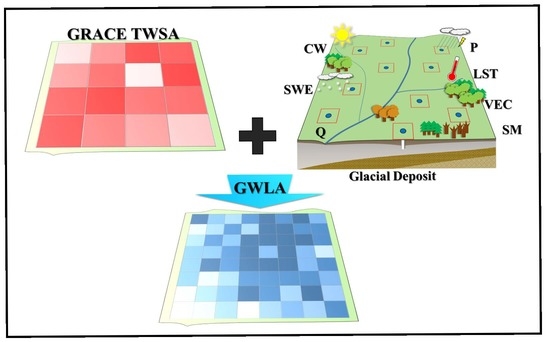
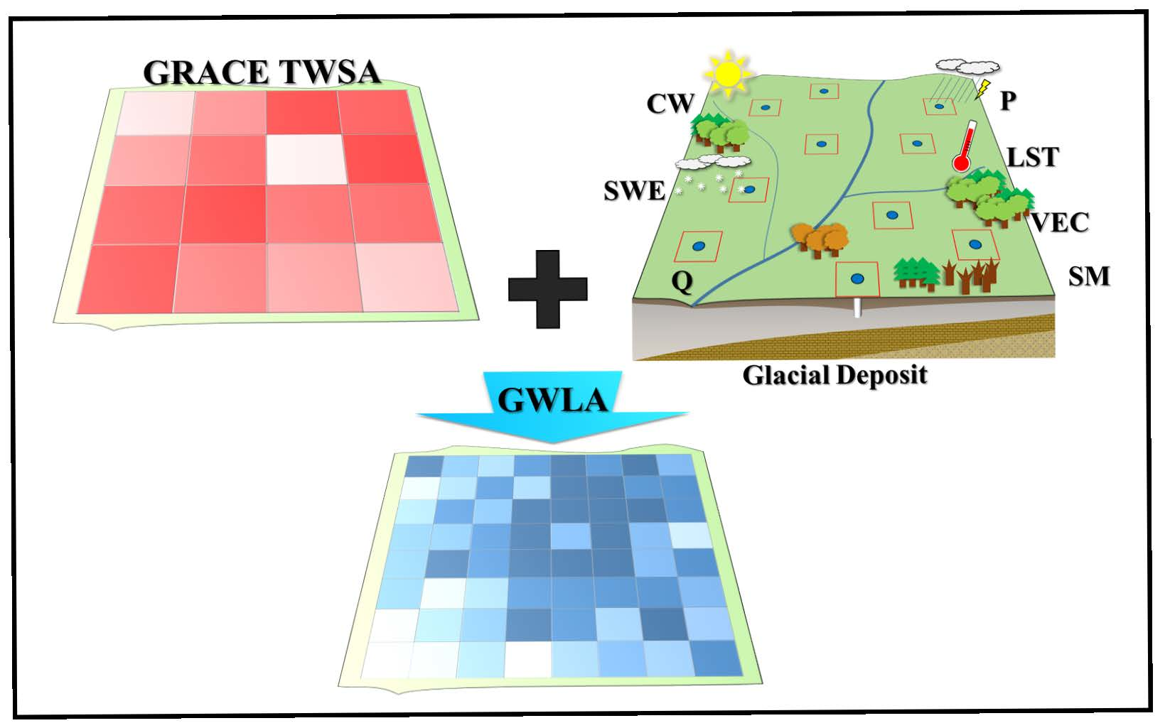
This study presents a machine learning approach to map high-resolution groundwater level anomaly (GWLA) from GRACE TWSA and other land surface and hydro-climate data (e.g., vegetation coverage, land surface temperature, precipitation, streamflow). A two-stage ML model: (1) Individual ML models for each groundwater level measurement station and (2) an ensemble model, which combines multiple ML models representing each well, was designed to predict high-resolution GWLA at a finer resolution than GRACE’s current resolution. Various publicly available satellite and model-based datasets were used to set up the downscaling model and were tested in time (2002–2016) and space (at 11 different locations) using in-situ groundwater level measurement data, which were excluded from model training. Predictor variables importance, interactions, and the influence of predictor variables on the predictand were analyzed in this study. In addition, GRACE TWSA averaged over the entire study area, TWSA from each 1°×1° grid, and TWSA average over a 3°×3° moving window were used and spatial randomization of the grids were implemented to test the effect of scale of GRACE data.
Previous research has demonstrated that storage in the vadose zone contributes to the total GRACE signal in some areas [
34]; however, due to the poor hydraulic characteristics of the glacial till, we assumed that the TWSA signal from GRACE is primarily dominated by groundwater. Therefore, the GRACE TWSA was directly mapped to groundwater storage anomaly. This minimizes further disaggregation of GRACE TWSA and reduces accumulation of errors associated with processing during the disaggregation of GRACE signal. Further, the downscaling approach was developed only considering the glacial aquifer system found covering the bedrocks in the study area, thus excluding the bedrock aquifers. This is because the bedrock aquifers are deep confined aquifer systems in most parts of the study area with little or no modern recharge, specifically in the central and southern parts [
35]. Therefore, the deep bedrock aquifers have less influence on the total water storage change from GRACE compared to the surficial glacial sediments.
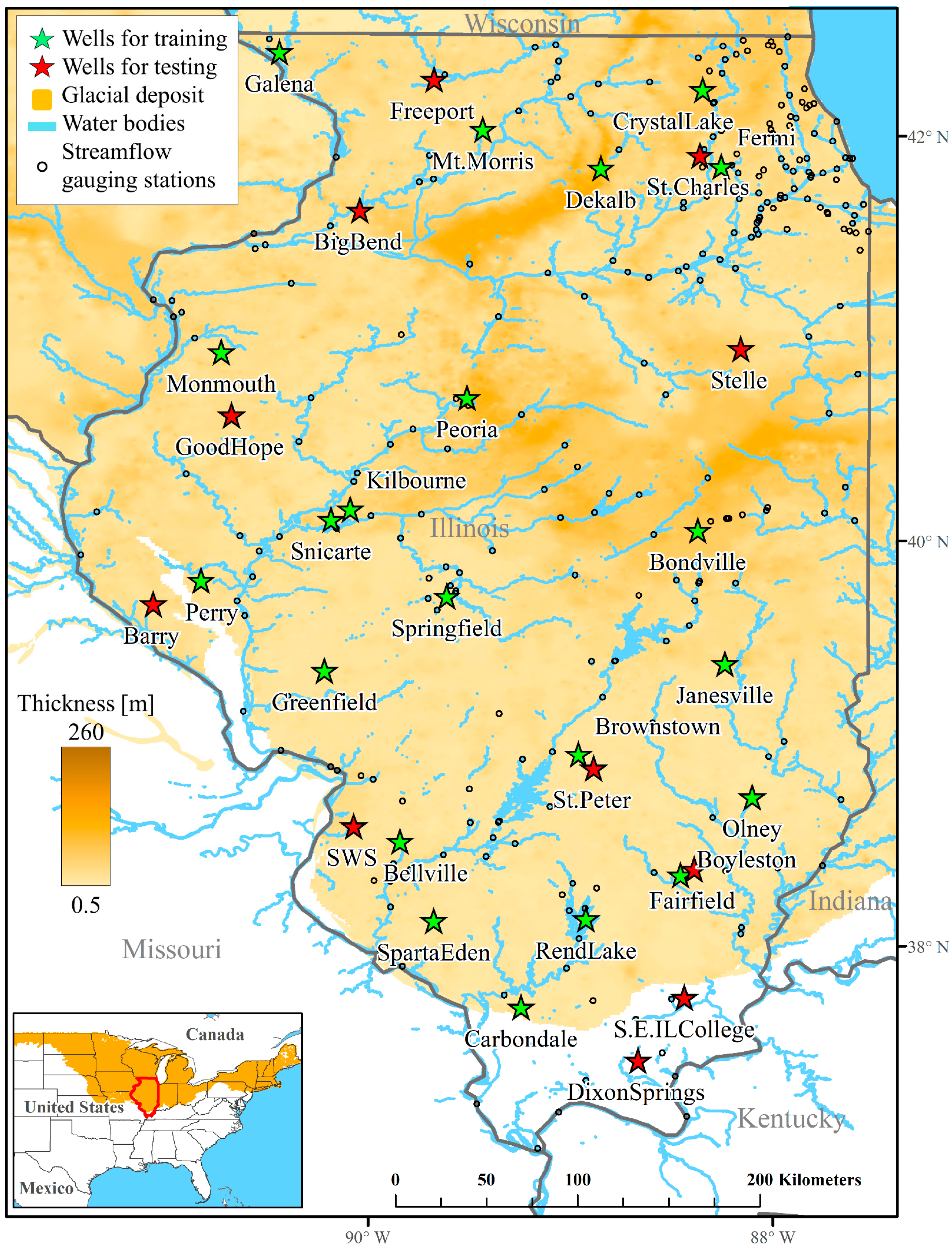
2.1. Study Area
The study area is located in the state of Illinois, a part of the Midwestern U.S., and covers an area of ~150,000 km
2 (
Figure 1). The surficial geology is mostly comprised of glacial drift sediments, while the land use is primarily rainfed agricultural row crop, corn, and soybeans. The major soil type in Illinois has a silty loam texture with a porosity of around 50%. Topographically, Illinois is characterized by mainly flat land with alternating ridges and plains (end moraines and till plains) in some areas that formed as a result of the retreating Wisconsin Episode glaciers [
36]. A continental climate with cold winters and warm summers characterizes the region. The long-term average annual precipitation of Illinois is ~960 mm, whereas the long-term mean, minimum, and maximum annual temperature of Illinois are 11 °C, 5 °C, and 17 °C, respectively [
37].
2.2. Data Source and Processing
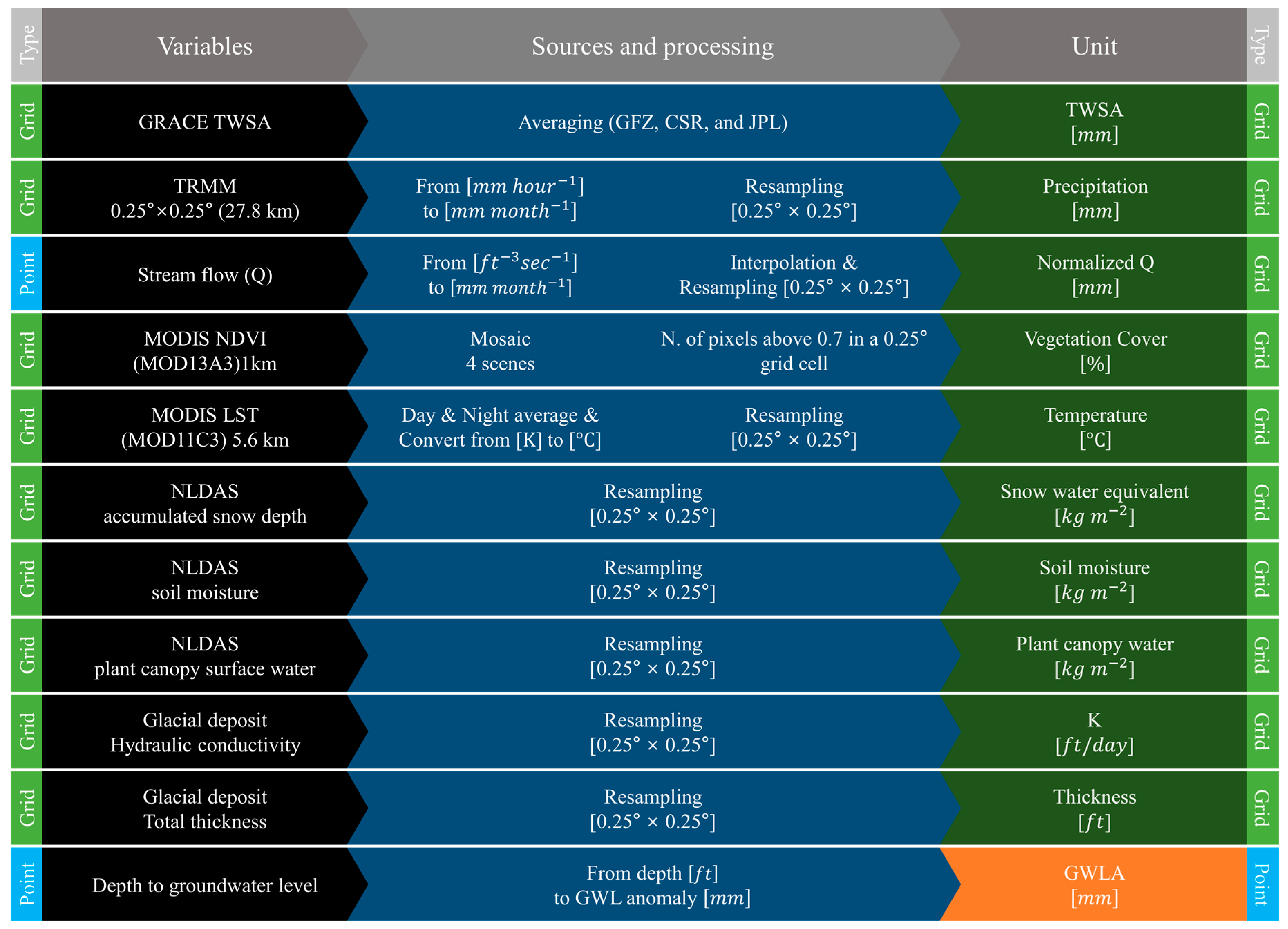
Ten predictor variables (e.g., TWSA, precipitation, vegetation cover, etc.) and one predictand variable (well-based groundwater level anomaly) were used to train and test the multi-stage ML models. The variables, data sources, and processing steps are summarized in
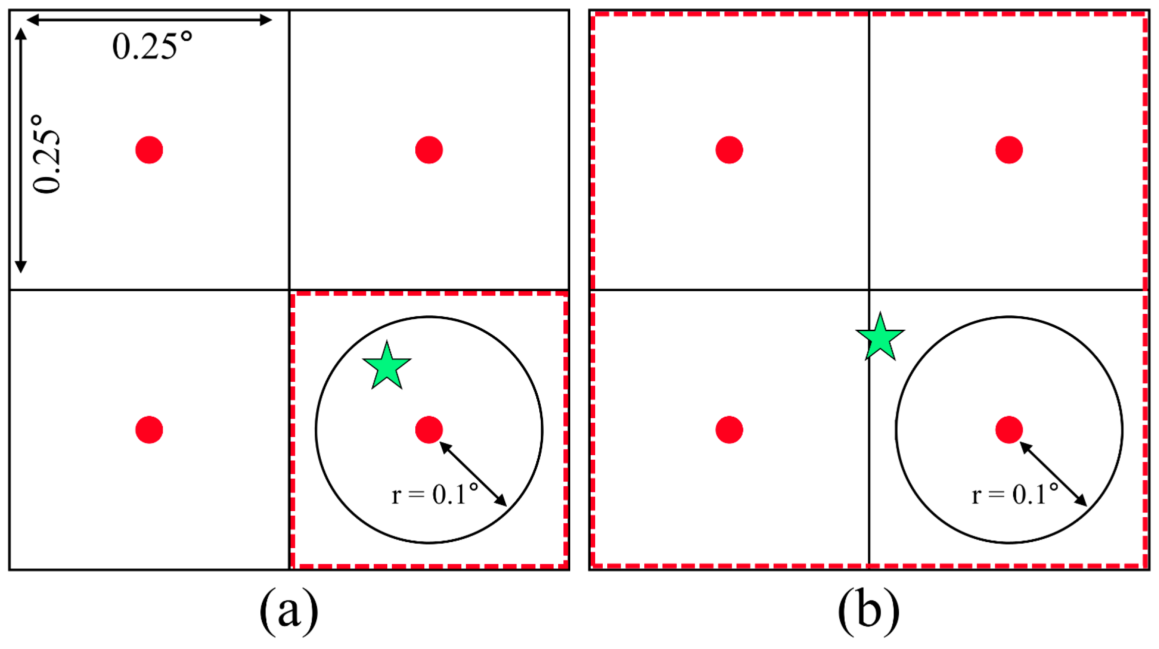
Figure 2, with details provided in the subsections below. All the data sources, with variable spatial and temporal resolutions were converted into uniform temporal (monthly) and spatial (0.25° × 0.25°) resolutions. Following the uniform resolution process, a distance weighted average scheme, based on the location of the groundwater level measurement stations, was implemented to extract timeseries input data from gridded raster datasets (
Figure 3). If a given groundwater level measurement station was within the threshold distance of 0.1° from the grid cell node (
Figure 3a), the value of that grid cell node was used as input data in to the model. However, if a groundwater measurement station was located outside of the threshold distance from the grid cell node, a distance weighted average scheme was used to get the average of the nearest four grid cell nodes surrounding the station (
Figure 3b).
2.2.1. Terrestrial Water Storage Anomaly (TWSA)
The GRACE mission, launched in 2002, is designed to track changes in the Earth’s gravity field using two identical satellites separated 220 km from each other at a 500 km orbital altitude [
38,
39]. GRACE detects change in gravity anomaly by using the high precision aboard instrument with the K-band ranging system capable of measuring the disturbance in orbital distances due to gravity variations (or mass changes) with an accuracy of 1 micron [
39]. After atmospheric and oceanic effects are accounted for, the remaining signal at a monthly timescale on land is mostly related to variations of terrestrial water storage [
40]. An ensemble mean of the latest release version (RL-05 gridded; 1° × 1°) level-3 GRACE product from three processing centers: The Center for Space Research at the University of Texas, Austin (CSR), the Jet Propulsion Laboratory (JPL), and the GeoforschungsZentrum Potsdam (GFZ) were used to ensure the highest level of accuracy [
27,
40]. To restore the signal attenuated during filtering and truncation of GRACE TWSA observations during processing [
40], the GRACE TWSA was multiplied by the scaling factor supplied with the GRACE data. The study time span is restricted by GRACE data availability that ranges from April 2004 to July 2016. GRACE land data are available at
http://grace.jpl.nasa.gov, supported by the NASA MEaSUREs Program [
40,
41].
2.2.2. Precipitation (P)
Precipitation data used in the model were obtained from the Tropical Rainfall Measurement Mission (TRMM) satellite. The TRMM Multisatellite Precipitation Analysis (TMPA) 3B43 product that provides monthly global (between 50 °N to 50 °S) precipitation intensity at 0.25° × 0.25° (~27.8 km) spatial resolution [
42] was used in the study. The TRMM 3B43 product is available on the web from NASA Giovanni (Geospatial Interactive Online Visualization and Analysis Infrastructure) service (URL:
https://giovanni.gsfc.nasa.gov/giovanni/; access date: 26 September 2017).
2.2.3. Stream Flow (Q)
Stream flow data used in the model was collected from the U.S. Geological Survey (USGS) streamflow database, the National Water Information System (NWIS) [
43]. The USGS dataRetrieval R package was used for retrieving daily stream flow data from the study area [
44,
45]. The daily flow rate (cms) for each station was converted into monthly discharges per unit area, with simplified units in mm per month, by considering the contributing drainage area of each gaging station. Further, this calculated point discharge per unit area data was linearly interpolated and resampled to obtain gridded raster discharge data at the appropriate scale. Location of gages used to get stream flow data is shown in
Figure 1.
2.2.4. Vegetation Coverage (VEC)
As vegetation plays a role in the terrestrial water storage, the Moderate Resolution Imaging Spectroradiometer (MODIS) satellite MOD13A3 (MODIS/Terra Vegetation Indices Monthly L3 Global 1 km SIN Grid V006) product that provides a monthly normalized vegetation index (NDVI) at a 1 km spatial resolution was used in the study [
46]. Four scenes (h10v04, h10v05, h11v04, and h11v05) of the MOD13A3 product covered the study area and were downloaded from the NASA Earth Data Search website (URL:
https://search.earthdata.nasa.gov/; access date: 28 August 2017). The mosaicked NDVI images were converted into percent vegetation coverage
using a threshold greenness index value of 0.7 [
27], percent greenness (NDVI ≥ 0.7) was calculated for each grid cell size of 0.25° × 0.25°.
2.2.5. Land Surface Temperature (LST)
Similarly, the MODIS MOD11C3 (MODIS/Terra Land Surface Temperature and Emissivity Monthly L3 Global 0.05Deg CMG) product was used to obtain monthly land surface temperatures. It has a 5.6 km spatial resolution (0.05°) [
47]. The earlier product versions (V4 and V41) of this data were used over the latest version (V5), because the algorithm used in V5 shows underestimation of LST under heavy aerosol condition [
48,
49]. Night and day LST layers of each monthly MOD11C3 were averaged into a single image to represent the mean temperature of a month. The MOD11C3 product is available on the NASA Earth Data Search website (URL:
https://search.earthdata.nasa.gov/; access date: 31 August 2017).
2.2.6. Snow Water Equivalent (SWE), Soil Moisture (SM), and Plant Canopy Water (CW)
Data for Snow Water Equivalent, Soil Moisture, and Plant Canopy Water were obtained from the Noah land surface model (LSM) based on the North American Land Data Assimilation System (NLDAS) [
50]. The NLDAS-2 monthly climatology Noah model provides information at a monthly time scale with a spatial resolution of 0.125° × 0.125° for the conterminous US. The products were downloaded from the NASA Giovanni (Geospatial Interactive Online Visualization and Analysis Infrastructure) service (URL:
https://giovanni.gsfc.nasa.gov/giovanni/; access date: 6 October 2017).
2.2.7. Drift Thickness (H) and Aquifer Characteristics (K)
Since aquifer heterogeneity is significant in the glacial deposit, integrating subsurface information about the aquifer material in the ML model is crucial. Gridded hydrogeologic properties for the glaciated United States were developed by Bayless, et al. [
51] from water-well drillers’ records. From this product, hydrogeologic information, such as hydraulic conductivity and thickness of the glacial deposits, was extracted and used in the model. The data can be obtained from the USGS’s Science Base website,
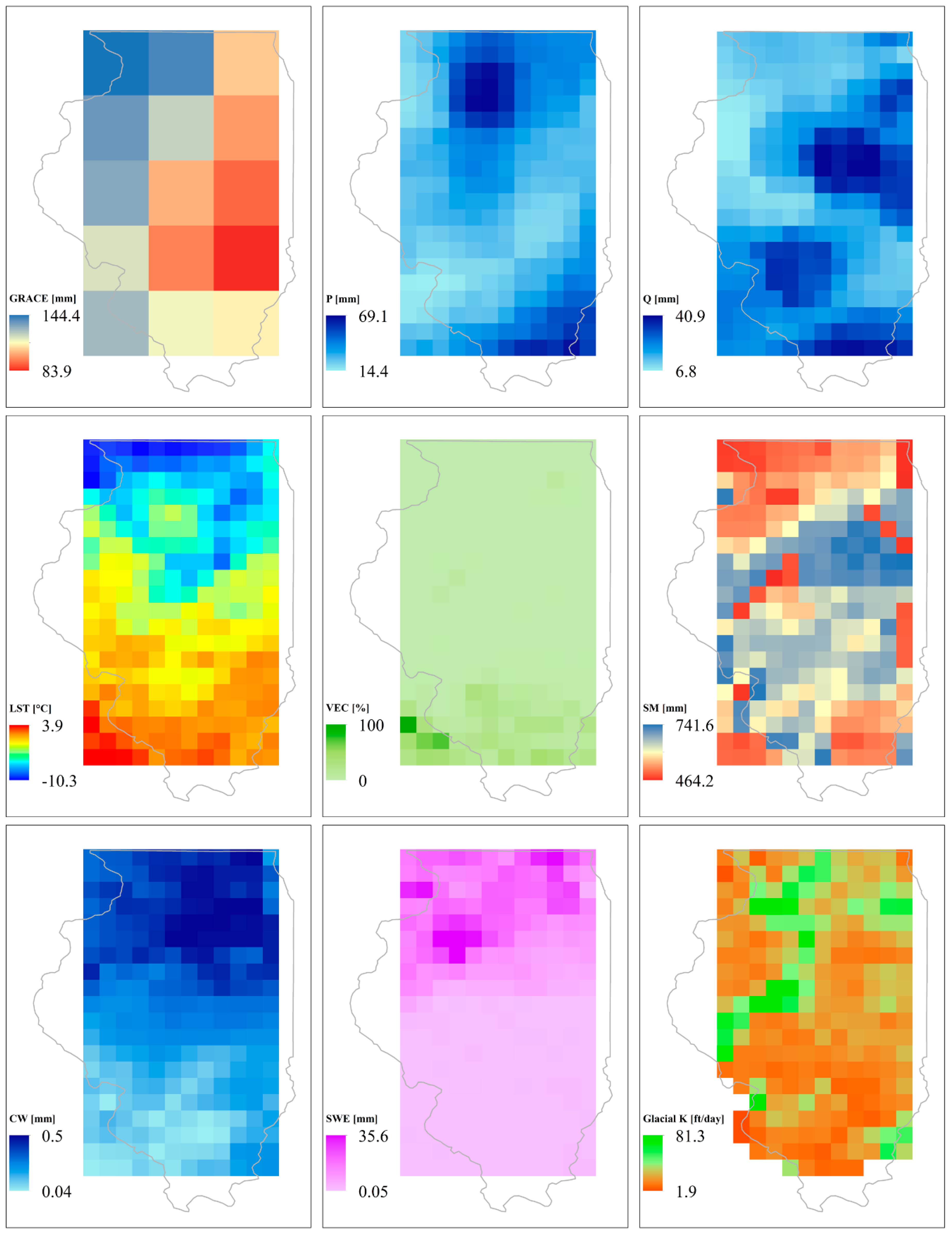
https://www.sciencebase.gov/catalog/item/58756c7ee4b0a829a3276352; access date: 8 August 2017). A sample gridded map showing all the input variables used in the methodology is shown in
Figure 4.
2.2.8. Groundwater Level Data (GWL)
In-situ groundwater level data were used as a target variable (predictand) in the ML model. Continuous groundwater level measurements are available from 32 stations in the study area, and were collected from the Illinois State Water Survey [
52]. Daily data were averaged into monthly groundwater level data. Furthermore, to mimic GRACE’s long-term anomaly data, the Groundwater Level Anomaly (GWLA) was calculated by subtracting the long-term average (according to GRACE’s long-term mean, 2004–2009) from individual GWL observations. The Shallow Groundwater Wells Network data is available on the Illinois State Water Survey website (URL:
https://www.isws.illinois.edu/warm/groundwater/: access date: 21 June 2017).
2.3. Modeling Algorithms
Downscaling GRACE to predict a high-resolution groundwater level anomaly and determination of variable importance was accomplished using a Boosted Regression Tree (BRT) also known as a gradient boosting technique. BRT, which is a combination of statistical and machine learning techniques, aims to improve the performance and prediction accuracy of a single tree-based model produced by fitting and combining a large number of tree-based models [
53,
54]. First, a sequence of several simple trees (weak models) is fitted to the data, and an ensemble (boosting) technique is applied to produce a robust model from several models [
53]. A tree-based method is conceptually simple yet powerful [
55] and has advantages over other predictive learning techniques in that the tree-based method is easy to interpret, handles missing values, is not affected by outliers and/or does not need prior data transformation, and it has the ability to deal with irrelevant inputs. For further details, refer to Friedman, Hastie and Tibshirani [
55] and Elith, Leathwick and Hastie [
53]. In addition, BRT works best with continuous and categorical data. The simplified theory of boosted regression method is briefly explained below.
Figure 5 shows how a tree-based regression divides a covariant space by partitioning the predictor variables [
56] and creates a simple tree-based model. A dataset space indicates a relationship between predictors (X
1 and X
2) and predictand (Y) so that the predictand value can be approximated by many rectangular subspaces (
Figure 5a) according to values of X
1 and X
2 and the splitting that forms the tree (
Figure 5b). The method builds binary trees that partition the data into two samples at each split node. The variable for splitting and its split value are selected based on the conditions that best fit the data. In the example in
Figure 5b, at first, the covariant space can be divided at X
1 = 8. This is based on the splitting (X
1 ≤ 8 and X
1 > 8) that can represent the covariant space most effectively in terms of residual error. Consequently, the second split points will be selected in both the X
1 ≤ 8 and X
1 > 8 regions. The number of split nodes determines the tree size; the increase in tree size is controlled either by a predetermined tree size or by residual error.
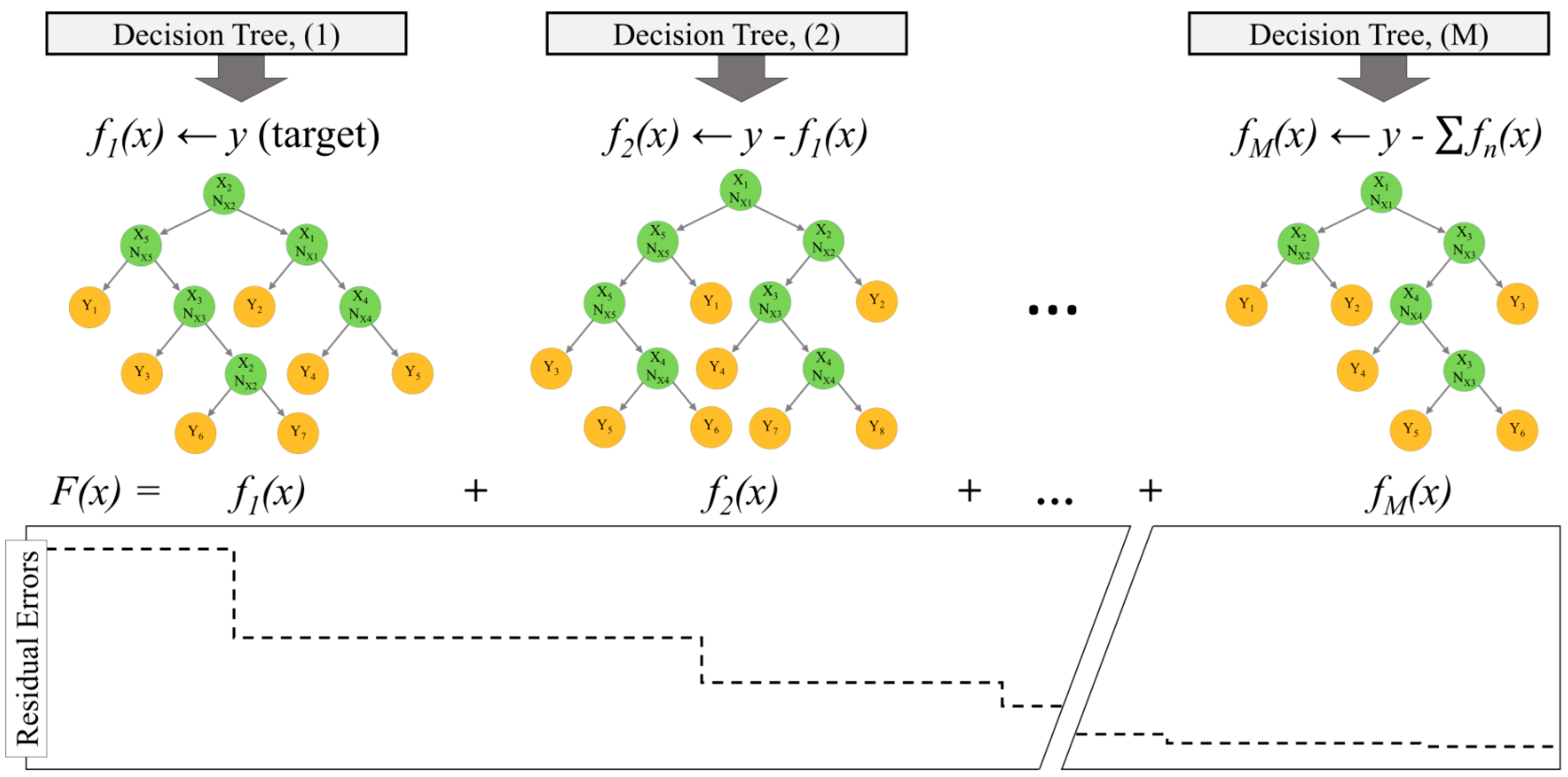
During boosting, a series of several simple trees is built based on the results of the prediction residuals of the preceding tree.
Figure 6 shows a schematic of successive regression trees based on residuals. As shown in
Figure 6, Decision Tree (2) is built based on a tree (partition) fitted to the residuals from Decision Tree (1), while Decision Tree (3) is a tree (partition) fitted to the residuals from Decision Tree (2). This helps to find a partition (Decision Tree (M)) that will further reduce the residual (error) variance for the data (as shown in the bottom graph of
Figure 6). As a result, boosting decision trees improves their accuracy, often dramatically [
55]. In boosting, decision trees are fitted iteratively to the training data and the algorithms vary in how they quantify lack of fit and select settings for the next iteration [
53]. In this study, LS Boost (least-squares regression) algorithm was used for BRT modeling (see Friedman [
57]). Optimization of hyperparameters (e.g., number of learners, maximum number of splits, and learning rate) (see Elith, Leathwick and Hastie [
53] for details) and overall model design and simulation was conducted using MATLAB
® 2017b. The model was constructed and tested using 10-fold cross-validation to determine the optimal hyperparameters, number of learners, maximum number of splits, and learning rate.
2.4. Downscaling Model Design
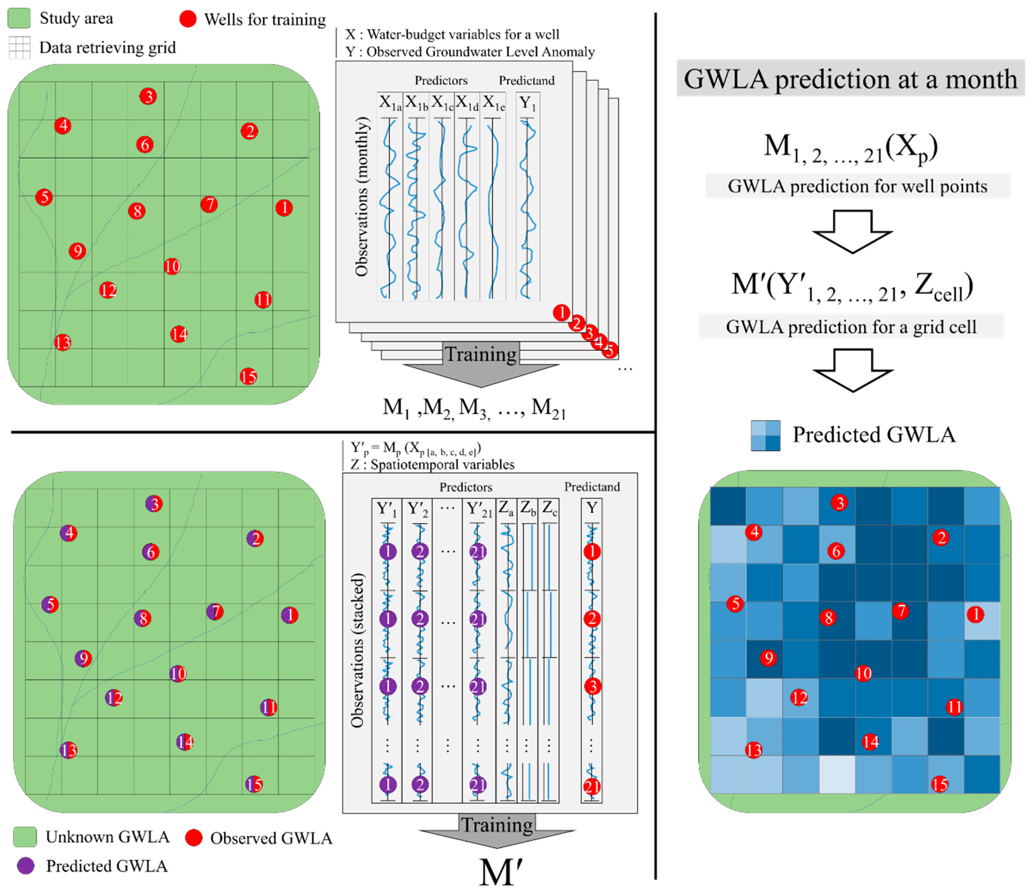
A two-stage ML approach was used in this study to generate a downscaled GWLA grid from GRACE TWSA. The first stage involved building multiple temporal GWLA prediction ML models (M
1, M
2, ..., M
21) for individual groundwater wells in the study area (top left section of
Figure 7). The second stage comprised of integrating these multiple models (from the previous stage), along with additional spatial information about the glacial deposit (e.g., hydraulic conductivity), into a single spatial downscaling model. In the second stage, a single spatial GWLA prediction model (M′) was produced for the entire study area (bottom left of
Figure 7) and used to generate a downscaled GWLA at 0.25° x 0.25° resolution (the right section of
Figure 7). As shown in the figure, the GWLA at a given month can be predicted (1) using GWLA predicted based on individual temporal models of training wells and water-budget variables (X) and (2) using two dimensional GWLA pattern generation based on intermediate variables (Y’) from the first models and spatial characteristics (Z) for each grid cell.
The GWLA prediction models in the first stage, in addition to GRACE TWSA, use terrestrial water cycle variables (e.g., vegetation coverage, LST, P, Q, SWE, plant canopy water, and soil moisture) (the specific variables used in each stage are shown in
Figure 2) as predictors, and in-situ-based GWLA as a predictand. While in the second stage, predictor variables are restricted to GRACE TWSA and aquifer characteristics (e.g., glacial thickness, hydraulic conductivity). Consequently, the spatial pattern of GWLA can be explained by glacial deposit characteristics in the second stage model.
The model was tested using data independent of training (calibration). Eleven groundwater well stations, excluded from the training sets, were used to test the performance of the spatial downscaling model (M′). The strength of the relationship between individual predictor variables and predictand was analyzed using variable importance (VI). The measure of variable importance is based on how many times the variable is selected for splitting and how much the model is improved as a result of the splitting (see Friedman and Meulman [
58] for details). Relative VI is calculated for each input variable and converted to a 0 to 100 scale. In addition, the sensitivity of each predictor variable was assessed using partial dependence plots that show the dependence between the predictand and a given predictor variable, while averaging the influence of all other predictors [
58].
During training and testing error metrics such as Mean (residual) Error (ME), Mean Absolute Error (MAE), Root-Mean-Square Error (RMSE), correlation coefficient (R), and Nash-Sutcliffe Efficiency (NSE) were used to evaluate the performance of the models by comparing model-simulated results with the observed GWLA.
3. Results
The results are presented according to the approaches applied in the downscaling procedure (2.4). Various GRACE grid sizes and spatial randomization of the GRACE grids were tested to standardize input from GRACE data and to test its effect on model accuracy. The results showed there is no clear improvement in the downscaling model. This could be due to the data where adjacent GRACE time series grids are highly correlated. As a result, the grid size and location have no impact in the model accuracy of the downscaling model. Lastly, the limitations of the method were discussed with respect to the actual condition in the study area; implications for future studies are also suggested.
3.1. Model Simulation Results
From the total of 32 groundwater level measurement stations in the study area, individual ML models were constructed for 21 of them, which were selected based on their spatial distribution. As the sample size, which is limited by GRACE sample size, was small to train the models, a ten-fold cross validation method was used. This method divided the entire data into ten subsets. Each subset was used nine times as a training set and one time as a test set. A model was fitted to the training set and evaluated based on the test set. As a result, the error estimation for model training was provided averaged over all trials to get the total effectiveness of the model.
Table 1 shows the overall statistics for model training of individual models (in the first stage ML models) and the ensemble downscaling model in the second stage. Generally, the results showed that the models exhibited excellent performances. The average ME, RMSE, R, and NSE values are 4.5 mm, 306 mm, 0.91, and 0.82, respectively. Similarly, the ensemble downscaling model shows an excellent performance with ME, RMSE, R, and NSE values of 0.0 mm, 192.0 mm, 0.98, and 0.96, respectively. Wells with good performance metrics (e.g., M7 and M10) imply the predictor variables explained well the observed GWLAs. On the other hand, wells with low performance metrics (e.g., M6, M12, M15, and M19) indicate that the predictor variables were short of fully explaining the observed GWLA. Note that the units are in mm for GWLA.
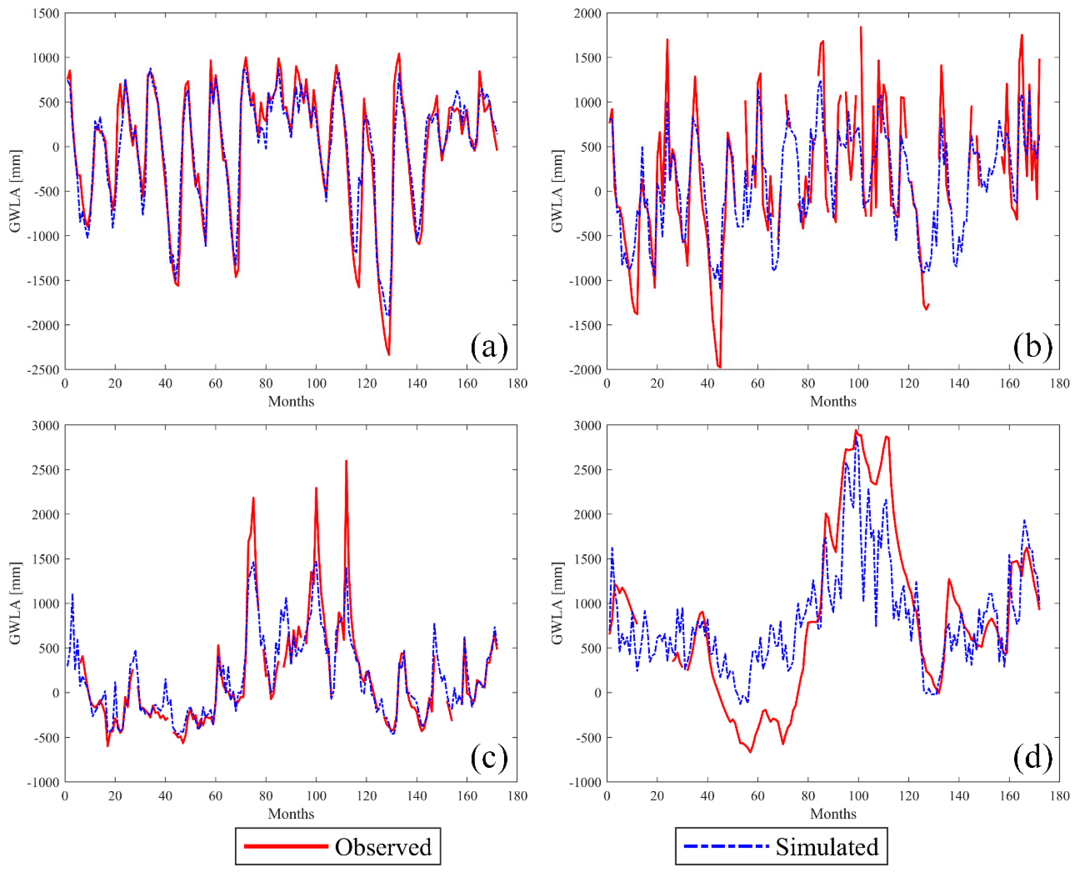
Figure 8 shows selected time series model-simulated GWLA vs in-situ-based GWLA. The models predicted the variation in GWLA very well for most of the groundwater measurement locations in the study area (e.g.,
Figure 8a). However, a few wells showed a slight underprediction (or overprediction) of the GWLA; specifically, underprediction in the picks of positive anomalies and overprediction in the picks of negative anomalies (
Figure 8b). Other exceptions include GWLA models for Galena (
Figure 8c) and Kilbourne (
Figure 8d) groundwater wells. Where the model for Galena station overpredicted the peak GWLA, whereas the model for Kilbourne station fairly captured the long-term GWLA variability; however, the model produced time-varying seasonal signal compared to the observed GWLA data. This is attributed to the fact that the Kilbourne well is located in an irrigated agricultural region of Illinois. Due to the lack of data, human impacts (e.g., pumping) were not considered as an input in this study. As shown in the figure, the hydrograph from the in-situ groundwater level data exhibited typical characteristics of pumping water level where little or no seasonal fluctuations were observed.
3.2. Variable Contributions and Sensitivity
Several studies indicated the GRACE signal is dominated by sub-surface storage (e.g., groundwater storage) [
59,
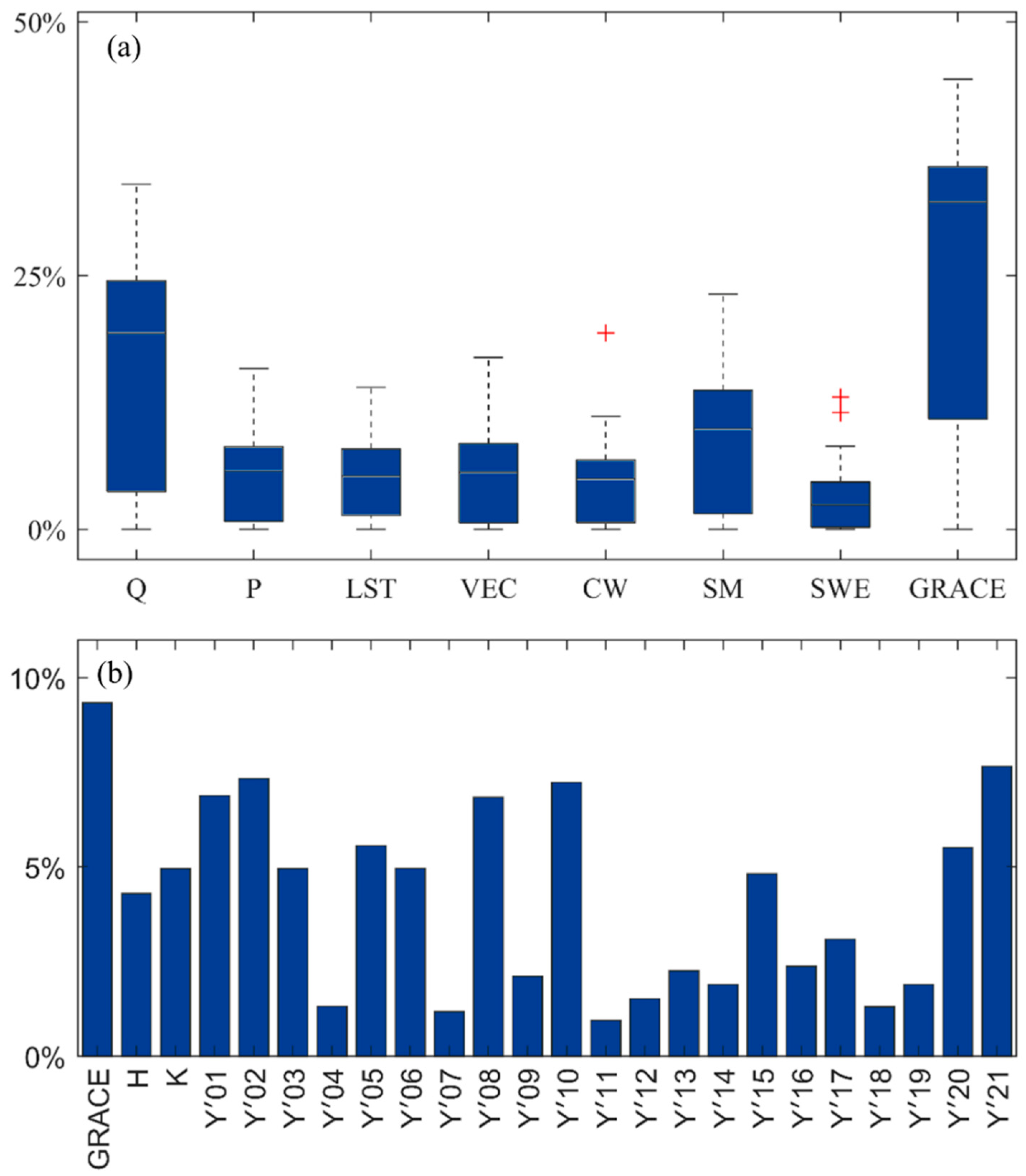
60]. The variable importance corroborated that TWSA from GRACE is an influential predictor variable of the predicted GWLA. Discharge is the second most important predictor variable. All the models (in both the first and second stages) indicated TWSA as a primary predictor variable (
Figure 9a,b) for the downscaled GWLA.
Figure 9a shows the percentage contribution of each predictor variable across all models in the first stage where individual models have been built for each groundwater level measurement station.
Figure 9b shows the percentage contribution of predictors in the second stage of the downscaling approach. In the first stage, stream discharge and soil moisture storage are the second and third most influential predictor variables, respectively. This can be explained by the glacial aquifer system in Illinois, which is mainly characterized by a shallow groundwater level, which influences baseflow contributions to the streams. The remaining predictor variables (e.g., precipitation (P), land surface temperature (LST), snow water equivalent (SWE)) are less and equally influential predictor variables. The relationship of these variables, though they directly or indirectly affect the amount of recharge to the groundwater, may not be simple and direct. In the second stage (downscaling model), the GRACE TWSA is relatively the most influential predictor variable, followed by a few predicted GWLA from the models in the first stage (
Figure 9b).
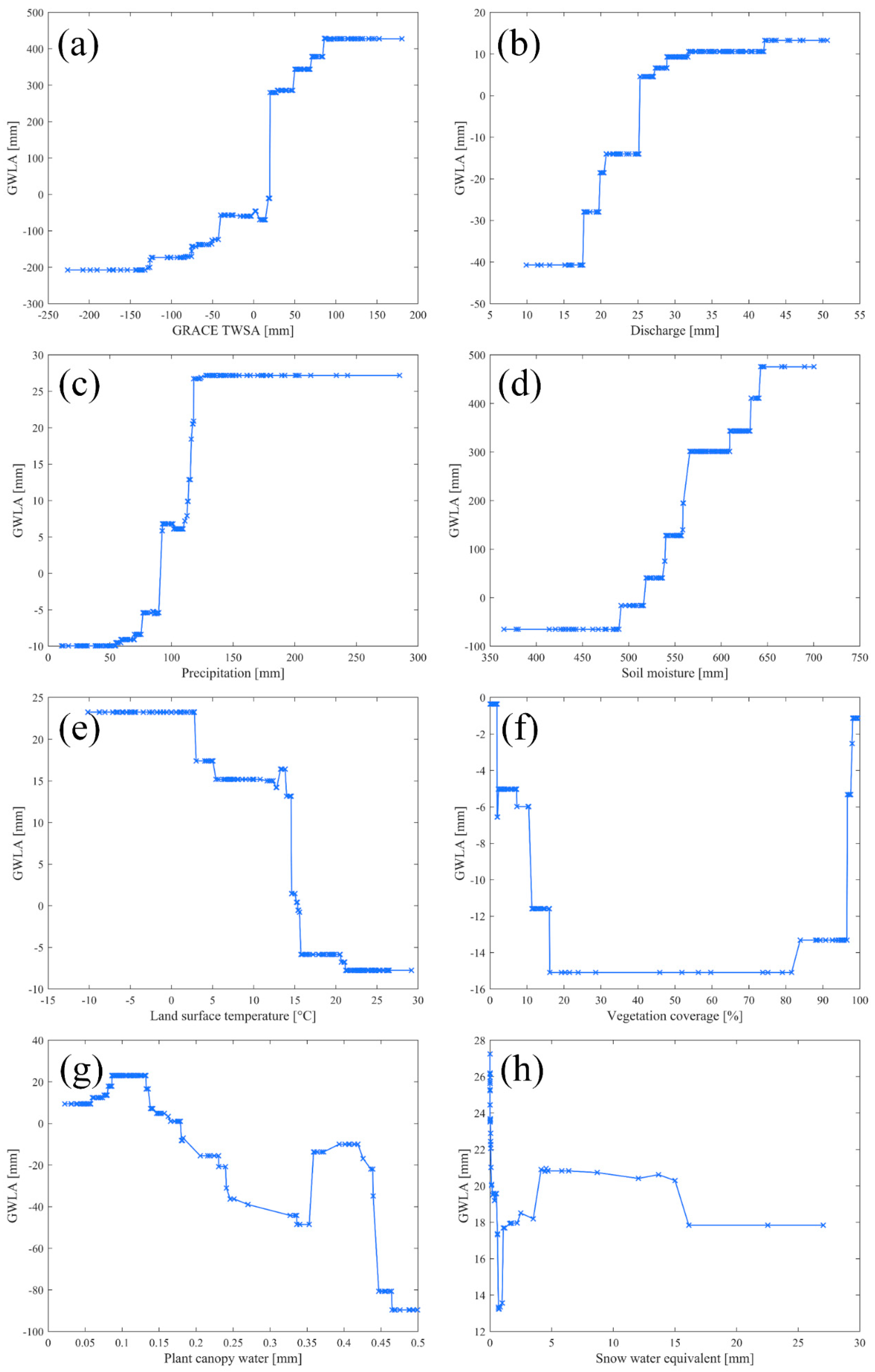
Figure 10 displays the Partial Dependence (PD) plots for selected models, which show the effect of a given variable on the response (predictand) after accounting for the average effect of all other predictor variables. Generally, there is a non-linear relationship between the predictor variables and the predictand (GWLA). The partial responses show a direct relationship between GWLA and GRACE TWSA, stream discharge, precipitation, and soil moisture. However, the magnitude effect of these predictor variables on the GWLA is different (see the y-axis of the graphs in
Figure 10). The GRACE TWSA and soil moisture control a wider range of the GWLA. The GWLA has an inverse relationship with land surface temperature and plant canopy water, as these predictor variables increase as the GWLA decreases. LST and CW favors evapotranspiration while reducing recharge. No clear relationship exists with vegetation coverage (greenness index) or snow water equivalent. The relationship between vegetation coverage and GWLA is not direct (
Figure 10f), where GWLA responds to little to no vegetation and high plant periods.
3.3. Testing and Spatial Accuracy
This study presents a novel approach that allows simulating higher resolution GWLA at different times and locations in space. The method was verified by comparing groundwater level data that was independent of model construction.
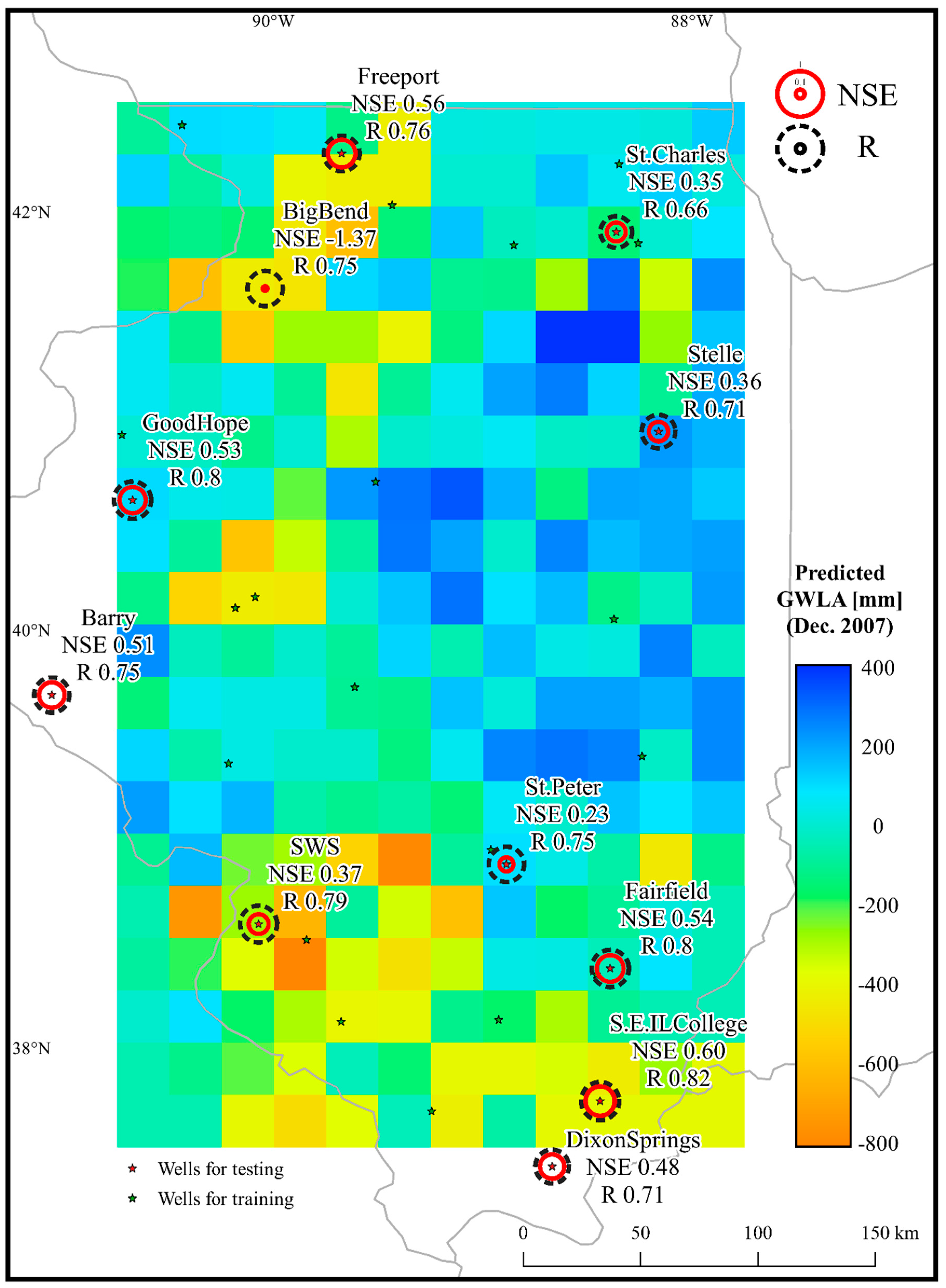
Figure 11 displays the distribution of test wells (red stars) and their statistical values (labeled next to the stations, the circles are also drawn to scale). Generally, the testing results showed that the statistical values are within the acceptable ranges. Half of the test wells have NSE values from 0.5 to 0.6, the remaining have values between 0.23 and 0.48. One well, Big Bend station, has shown a very low NSE value of −1.37; however, it has a high correlation coefficient value of 0.75. This well is located within the floodplain of the Rock River where the groundwater interacts with the river via baseflow. The direction of seasonal fluctuation (indicated by high correlation coefficient) can be simulated well by the downscaling model mainly influenced by stream discharge. However, the model falls short of predicting the magnitude of the GWLA compared to the observed GWLA data, which is different from the magnitude of discharge. Generally, the correlation coefficients for testing are within the range of 0.66 to 0.82. The test results show that the downscaling approach presented here satisfactorily simulates the GWLA data at 0.25° × 0.25° spatial and monthly temporal scale from GRACE. The output scale is defined based on the scale of input data. TRMM has the lowest resolution of the input data at 0.25° × 0.25°. Though not tested in this study, it is possible to downscale further to a higher resolution using high-resolution input data.
The background image in
Figure 10 shows a sample-predicted GWLA (for the month of December 2007) for the study site at 0.25° × 0.25° resolution. We can see that there is significant GWLA spatial variation during that month. A negative groundwater level anomaly of more than 500 mm (areas in yellow and red) was observed in the southern and northwestern parts of the study site, whereas the north and northeastern parts gained a positive groundwater level anomaly up to 500 mm (areas in blue). Overall, the similar degree of heterogeneity in groundwater behavior is observed in other months from model output compared to that of GRACE data.
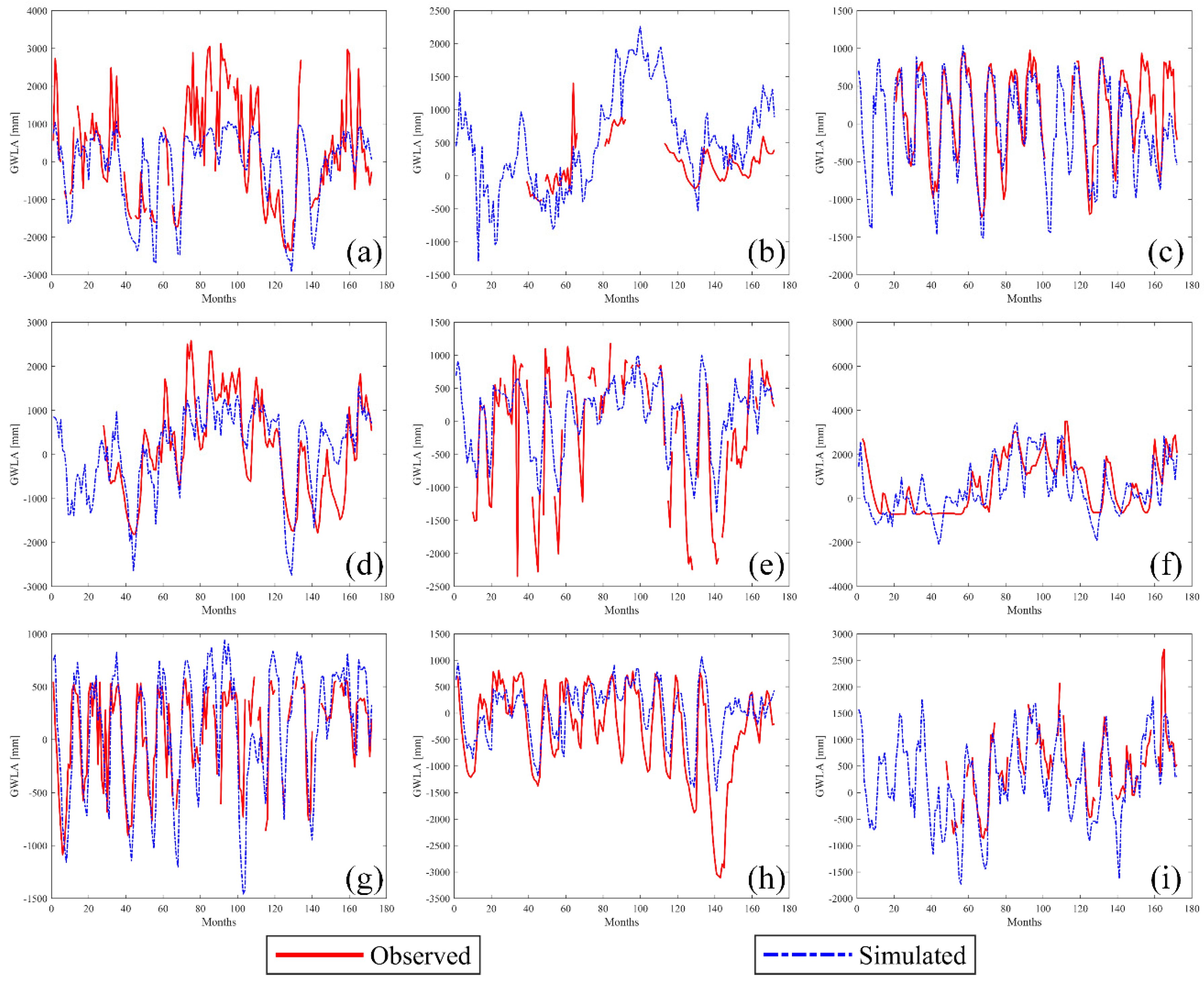
Figure 12 shows the timeseries model-predicted versus in-situ-derived GWLA for each test well in the study area. Differences in model performances are observed between different test wells; good predictive performances are observed in, e.g., test wells at Fairfield and Freeport stations (
Figure 12c,d) and poor performance in the test well at Big Bend station (
Figure 12b). As seen in
Figure 12, Big Bend station data availability is low, resulting in poor NSE and R values for this station due to sample size. In some of the test wells, the model underestimates the GWLA (e.g.,
Figure 12a,d,e). The reverse, an overestimate of the GWLA, is observed in the St. Peter test well data (
Figure 12g). Generally, the model predicted the timing and seasonal variability (direction) of the GWLA. However, in some instances (as described above), the model less accurately predicted the magnitude of the high and low groundwater anomalies. This is due to the skill of the models mainly controlled by input data, specifically, data for the predictor variables. The authors believe the variances in the predictor variables may not be capable of fully explaining the magnitudes of variability in the predictand variable (GWLA). Despite some limitations, as indicated by the statistical measures above (
Figure 11), the model predicts the monthly variations in the groundwater level moderately well and better predicts the long-term (seasonal to interannual) variability in the groundwater level. For example, in stations such as Barry, Big Bend, Freeport, Good Hope, and SWS (
Figure 12a,b,d,e,i), the model predicted the dry anomalies (e.g., periods from 40 to 60 and 120 to 140) and wet anomalies (e.g., periods from 80 to 120).
4. Discussion
Overall, the approach developed in this study demonstrates the integration of satellite- and model-based hydrological variables along with GRACE data to predict high-resolution groundwater level variation in a glacial aquifer system. The results clearly demonstrate that downscaled GWLA could be predicted at a resolution of 0.25° × 0.25° in new periods and/or space in the study area, a limiting factor in previous studies. Additional tests have been conducted to increase replicability of this study, such as testing the spatial scale of input variables (e.g., GRACE grid). Using the methodology developed in this study (a generic code is available from the authors upon request), end-users can implement it elsewhere to predict GWLA, given all the assumptions are valid. The two main assumptions are (1) GRACE TWSA is mainly controlled by the groundwater storage variation in the shallow aquifer system and (2) human influence (e.g., groundwater abstraction for irrigation from the aquifer) is not considered as an input variable in the models.
The purpose of using publicly available data (e.g., satellite data) is to establish the applicability of this study in data-scarce regions where hydrologic variables are limited, such as lack of groundwater recharge rate and poorly distributed well data in space and time. However, significant uncertainty is expected from these data sources. For example, GRACE data has its own uncertainty that arises from GRACE processing. Other input data, some model-based and satellite-based, have their own contribution to the total input data uncertainty and potential error propagation. These errors are mitigated by using ML methods, as they do a good job of handling errors associated with input data.
Only the shallow groundwater system of the glacial sediment was considered in this study by assuming the GRACE signal is strongly related to shallow systems. As a result, shallow bedrock aquifers overlain by no or thin layers of glacial sediment, specifically in the northern part of the study area, were not included. The authors believe that the poor performance of the ML model in this part of the study region (e.g., at Crystal Lake and Fermi stations (see
Table 1 and
Figure 1)) could be due to exclusion of the shallow bedrock. Further, exclusion of human impact as a predictor variable has also affected the performance of wells located in the irrigated regions of Illinois (e.g., Kilbourne and Sincarte wells) where the main source of irrigation water is groundwater. As it has been seen in the hydrograph of Kilbourne stations (
Figure 8d), the in-situ groundwater data shows more of a flat declining or rising groundwater level anomaly; however, the model that simulated the natural seasonal fluctuations was probably influenced by seasonal variability of precipitation and other predictor variables. Further, the spatial pattern of groundwater level anomalies may not be fully captured due to heterogeneity of the glacial system. The predictor variables used in this study may not be used to sufficiently describe this heterogeneity in order to predict the GWLA accurately in these instances. Adding more variables (e.g., storage characteristics of the aquifer, including the bedrock), as well as improved resolution of the input variables, potentially minimizes the bias and improves the prediction capacity of the ML model.
The methodology developed in this study can be directly applied in shallow sedimentary aquifer systems with similar settings where (1) GWLA response to climate variables is relatively quick and (2) anthropogenic influences (e.g., groundwater abstraction) are not extensive. For example, the downscaling model can be applied in the Chad Basin, the Congo Basin, and the Rift Valley Basin in Africa. The central part of the Chad Basin has a Quaternary unconfined sediment aquifer system made up of fluvio-lacustrine deposits and Aeolian sands and covers an area of 500,000 km
2 [
32]. This basin is one of the most poorly gauged basin in the world but provides fresh water resources for the people of several nations in the region. Similarly, it can also applied in the fluvio-lactustrine sediment aquifers covering the Rift Valley in East Africa and the Cenozoic sediment aquifers in the Congo Basin, among others.
To apply the methodology in a different setting, it is possible to omit or include predictor variables. For example, snow water equivalent and vegetation coverage are insignificant in arid regions. As a result, researchers can omit these predictor variables from the downscaling model. Likewise, if additional variables are necessary to explain the predictand variable, they can be easily included as predictor variables. For example, if the geological setting is a fractured (Karstic) bedrock aquifer system, it is possible to include additional predictor variables, such as fracture density and fracture spacing, to explain the predictand variable, the GWLA. In addition, as BRT works well with both categorical and numerical variables, it is possible to include categorical data (e.g., yes or no type data or qualitative data) by assigning numeric values such as 0 (no) and 1 (yes).
5. Conclusions
With continued threat from climate change and human impacts, high-resolution and continuous hydrologic data availability is crucial for predicting trends and water resource availability. GRACE has provided unprecedented opportunities to assess regional and global water resources, despite the limitations due to its coarse spatial scale. This study presented a two-stage machine learning approach to map high-resolution groundwater level anomaly (GWLA) from GRACE TWSA and other publicly available land surface and hydro-climate data (e.g., vegetation coverage, land surface temperature, precipitation, streamflow, etc.) in a glacial aquifer system in Illinois. In both stages, the models were validated and tested. The study finds GRACE to be the most influential predictor variable in the ML-based models, and the scale of GRACE or spatial location of GRACE grids have little to no impact on the performance of the ML-based downscaling model. This is due to the characteristics of GRACE grids, where they have a coarse resolution and where adjacent GRACE grids are spatially highly correlated. Stream flow and soil moisture storage are the second and third most influential predictor variables in the model.
Generally, the model training and testing results, in the first stage, showed excellent performances. The average ME, RMSE, R, and NSE values are ~4.5 mm, 306 mm, 0.91, and 0.82, respectively. Similarly, the ensemble downscaling model (in the second stage) shows an excellent performance with ME, RMSE, R, and NSE values of 0.0 mm, 192.0 mm, 0.98, and 0.96, respectively. Further, the downscaling model was tested satisfactorily using the monthly in-situ-based GWLA data excluded during model construction. A few test wells exhibit relatively poor statistical performances, which is attributed to the lack of anthropogenic influences (e.g., pumping) in groundwater-irrigated regions and insufficient representation of aquifer heterogeneity in the predictor variables. Various sources of uncertainties in the model and downscaled product are expected, such as uncertainty from the input satellite and model-based data and uncertainty from the model assumption (e.g., exclusion of the shallow bedrock aquifer system located in the northern part of the study area). However, noises due to input data were often reduced (or minimized) during the machine learning process.


