Method to Reduce the Bias on Digital Terrain Model and Canopy Height Model from LiDAR Data


1
Department of Wood and Forest Sciences, Université Laval, Quebec City, QC G1V 0A6, Canada
2
Direction des Inventaires Forestiers, Ministère des Forêts, de la Faune et des Parcs du Québec, Quebec City, QC G1H 6R1, Canada
*
Author to whom correspondence should be addressed.
Remote Sens. 2019, 11(7), 863; https://0-doi-org.brum.beds.ac.uk/10.3390/rs11070863
Submission received: 5 March 2019
/
Revised: 3 April 2019
/
Accepted: 7 April 2019
/
Published: 10 April 2019
(This article belongs to the Special Issue 3D Point Clouds in Forests)
Abstract
:Underestimation of LiDAR heights is widely known but has never been evaluated for several sensors and for diverse types of ecological conditions. This underestimation is mainly linked to the probability of the pulse to reach the ground and the top of vegetation. Main causes of this underestimation are pulse density, pattern of scan (sensors), scan angles, specific contract parameters (flying altitude, pulse repetition frequency) and characteristics of the territory (slopes, stand density and species composition). This study, carried out at a resolution of 1 × 1 m, first assessed the possibility of making an adjustment model to correct the bias of the digital terrain model (DTM), and then proposed a global adjustment model to correct the bias on the canopy height model (CHM). For this study, the bias of both DTM and CHM were calculated by subtracting two LiDAR datasets: high-density pixels with 21 pulses/m2 (first return) and more (DTM or CHM reference value pixels) and low-density pixels (DTM or CHM value to correct). After preliminary analyses, it was concluded that the DTM did not need specific adjustment. In contrast, the CHM needed adjustments. Among the variables studied, three were selected for the final CHM adjustment model: the maximum height of the pixel (H2Corr); the density of first returns by m2 (D_first); and the standard deviation of nine maximum heights of the neighborhood cells (H_STD9). The modeling occurred in three steps. The first two steps enabled the determination of significant variables and the shape of the equation to be defined (linear mixed model and non-linear model). The third step made it possible to propose an empirical equation using a non-linear mixed model that can be applied to a 1 × 1 m CHM. The CHM underestimation correction could be used for a preliminary step to several uses of the CHM such as volume calculation, forest growth models or multi-temporal analysis.
1. Introduction
Airborne LiDAR (Light Detection and Ranging) has been beneficial in the field of forestry for several years because of its ability to produce very accurate information about terrain [1,2]. Among the information obtained from LiDAR data, vegetation height is an important variable for forest management. Furthermore, metrics related to height are key explanatory variables for many attributes such as volume [3,4,5] or biomass [6,7]. The height is therefore used extensively, despite the fact that it is well known for underestimation [8,9].
Several measurable factors have been proposed to explain underestimations, including: (i) pulse density, (ii) pattern of scan (sensors), (iii) scan angles, (iv) contract specific parameters (flying altitude, pulse repetition frequency), (v) territory characteristics (stand density and species) and (vi) ground overestimation [10,11,12,13,14,15,16,17,18,19,20,21,22,23,24,25,26,27,28].
Lefsky et al. [25] determined that pulse density is the principal parameter determining tree height underestimation. According to several other studies, pulse density has an impact on underestimations of height, depending on the scale of the study and on the mean pulse density of the LiDAR survey. Bater et al. [24] analyzed, at plot scale, the impact of different pulse densities at the maximum height, and concluded that maximum height was significantly different between pulse densities varying within 2% to 4%. Treitz et al. [23] also studied the impact of pulse density (3.2 pulses/m2 decimated to 0.5 pulses/m2) on several forest inventory variables such as tree top height, but concluded that at plot scale, the pulse density had no significant effect on tree top height. Furthermore, at a tree scale, Sibona et al. [17] concluded that heights obtained by LiDAR were not significantly different to those measured in the field for pulse densities higher than 5 pulses/m2. Moreover, Yu et al. [27] demonstrated that height underestimation increased as the pulse density decreased and that the underestimation between 2.5 and 5 pulses/m2 was greater than between 5 and 10 pulses/m2. Additionally, Naesset & Okland [26] stated that the most efficient way to increase the height precision is by increasing the pulse density. Finally, Roussel et al. [10] demonstrated that at a 4 m2 scale, for a pulse density of 21 pulses/m2 or higher, underestimation would be smaller than 0.10 m. The authors also analyzed the scale effect and concluded that for the same density, the scale also significantly impacted the underestimation [10].
Other parameters may also influence the underestimation of the height. First, the scan pattern used influences the distribution of pulses and therefore the pulses/m2. Optech and Leica sensors use oscillating mirrors, while Riegl uses a rotating polygon. The first category produces zigzag scan lines (heterogeneous distribution of pulses), while the second uses parallel scan lines (homogeneous distribution of pulses) [11]. Second, scan angles influence the estimation of forest height. The effect of this factor is different, depending on the forest structure [12]. For example, Holmgren et al. [13] simulated four different forest types to evaluate the underestimation caused by scan angles. Their results show that long crown species like spruce are more affected than short crown species like pine. Furthermore, dense stands are less affected than sparser stands. Montaghi [14] compared scan angles at nadir with scan angles between 0 to 20 degrees, and concluded that scan angles smaller than 20 degrees have no significant impact on stand measured height. Third, higher flying altitudes or increased pulse frequencies reduce the pulse intensity, and thus, require larger and denser backscatter areas to return the pulse to the sensor. Ultimately, lower pulse intensities increase the pulse penetration into foliage, and thereby, underestimate height [15]. Hopkinson [15] varied pulse intensities between surveys for 24 plots and demonstrated that decreasing pulse intensity lead to an increase in foliage penetration varying from 0.15 to 0.61 m with other parameters remaining constant. Fourth, height underestimation is also influenced by crown shape [16], stand density and species composition [8,17,18]. Sibona et al. [17] showed between three species that European larch had the smallest mean absolute difference (0.95 m) compared to scots pine and European spruce, which had respective underestimations of 1.4 m and 1.13 m. Furthermore, Yu et al. [27] demonstrated that underestimation varied according to species. In order, pine is the most affected, followed by spruce and birch. Finally, height underestimation is also influenced by an overestimation of the digital terrain model (DTM). Hyyppä et al. [28] demonstrated that DTM error varies according to slopes, undergrowth vegetation and forest cover type. Indeed, slopes can lead to overestimations, in part due to beam divergence. Beam divergence has a greater effect on steep slopes than on flat ground. This divergence causes horizontal errors, and consequently, on steep slopes, vertical errors [19,28]. Tinkham et al. [19], for example, demonstrated that a slope greater than 30 degrees has a significant vertical DTM error and that vegetation structure has no significant impact on the DTM values. Also, Hyyppä et al. [28] demonstrated that DTM accuracy gradually decreases as the slope increases. Furthermore, the authors show that resulting DTM error in forested areas is greater than in open areas. Finally, dense stands [20] and understory vegetation [21] increase DTM overestimations.
In conclusion, factors influencing the precision of altitude values from airborne LiDAR depend on two main elements: (i) the capability of the pulse to reach the ground [19,22], and (ii) its probability to hit the canopy. Both phenomena are analyzed in this work in order to evaluate their quantitative impacts and to calculate models to correct the resulting difference between the reference value and the value to correct (here and after called bias).
The goal of this study is first to propose an adjustment model to correct the DTM bias, and ultimately, to propose an adjustment model to correct canopy height model (CHM) bias for a wide range of site and acquisition conditions. Although several factors have been evaluated separately, no study has accurately measured these factors and proposed adjustments on DTM and CHM in a variety of forest conditions.
2. Materials and Methods
2.1. Study Area
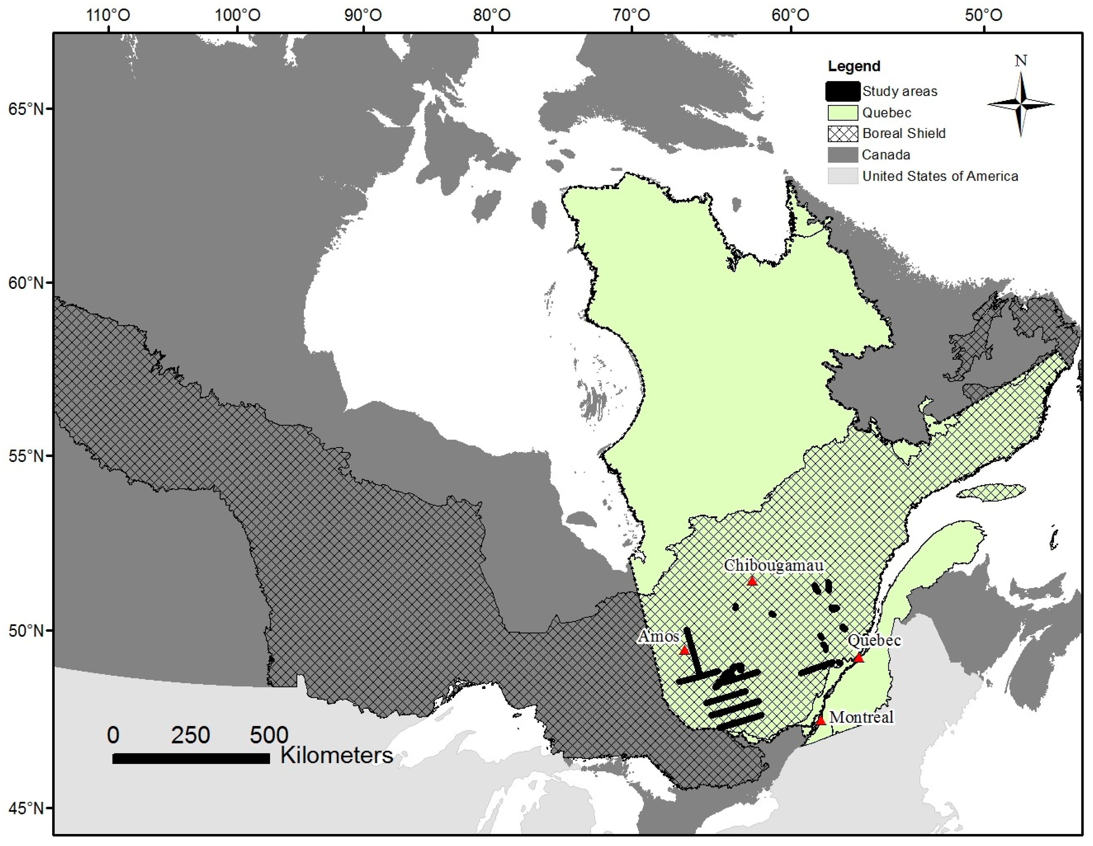
A total of 29 study sites covering more than 3500 km2 were selected over a large spectrum of climatic, topographic and ecological conditions existing in the boreal shield ecozone (Figure 1). Each site is covered by two different LiDAR datasets acquired within half of a growing season in order to minimize the differences caused by vegetation growth. All study sites were located in the province of Quebec, Canada (Figure 1).
The main forest species in the study areas were black spruce (Picea mariana (Mill.) B.S.P.), white birch (Betula papyrifera Marsh.) and balsam fir (Abies balsamea (L.) Mill.). Several other species were present, such as trembling aspen (Populus tremuloides Michx.), jack pine (Pinus banksiana Lamb.), sugar maple (Acer saccharum Marsh.), yellow birch (Betula alleghaniensis Britt.), tamarack (Larix laricina (Du Roi) Koch.), white pine (Pinus strobus L.), white spruce (Picea glauca (Moench) Voss) and red maple (Acer rubrum (L.). The study areas were found along a vegetation gradient. From the north to the south, coniferous (black spruce, balsam fir, tamarack), mixed (balsam fir, white birch, trembling aspen, yellow birch) and deciduous (sugar maple, yellow birch) tree stands were found. A wide range of forest attributes and ecological conditions were also covered, as shown in Table 1.
2.2. LiDAR Data
A total of 30 different airborne LiDAR datasets covered the 29 study sites where some LiDAR datasets covered more than one site. Main selection criteria were based on the availability of two airborne LiDAR datasets for the same area within less than half a growth year. These surveys were acquired between 2011 and 2017 using discrete return sensors 1064 nm in wavelength. All were conducted in full leaf conditions with overlap between flight lines ranging from 20 to 30%. All acquisitions had to fulfill accuracy requirements: 0.25 m in XY and 0.50 m in Z axes. The different characteristics of each sensor are described in Table 2.
2.3. Rasterization
2.3.1. Selection of Resolution
First, working in raster format (DTM and CHM) eliminates the noise due to the choice in the tree detection algorithm. Kaartinen et al. [36] compared 13 different algorithms in boreal forest conditions and demonstrated that the chosen algorithm is the main factor influencing tree detection. Wallace et al. [37] evaluated the influence of point density in tree detection and concluded that a minimum density of 5 pulses/m2 is necessary for individual tree level analysis which is higher than the density used in this study.
Inspired by Vepakomma et al. [38], the optimal grid resolution determined was chosen and relied on two criteria: (1) to have a minimum number of raster pixels without any return and (2) to have a maximum number of pixels with 21 pulses/m2 or more. For all of the 30 different airborne LiDAR grid datasets, rasters were produced with two grid resolution (1 × 1 m and 2 × 2 m). For this study, 1 × 1 m resolution was chosen for all rasters.
2.3.2. Generation of the Rasters
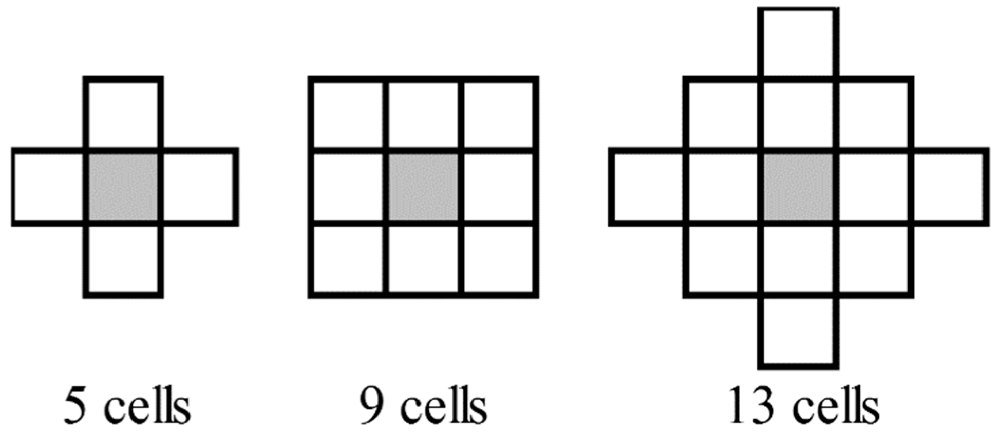
First, ground and non-ground LiDAR returns were classified with LAStools algorithms (Rapidlasso, GmbH). No filter was applied and the basic settings were preserved. For each of the two datasets covering a study site, a DTM (reference DTM (DTM_ref) and DTM to correct (DTM2Corr)), a canopy surface model (CSM) and some of the LiDAR variables detailed in Table 3 were rasterized by LAStools. DTM was defined as the central altitude value of each pixel obtained by the linear interpolation of ground returns triangulation and CSM as the altitude value of the highest return (all returns) by m2. The height value comprised in CHM (reference height (H_ref)) and height to correct (H2Corr)) were obtained by subtracting the DTM from the CSM. Because the forest structure influences the height bias [12,13], the maximum height standard deviation was tested as a forest structure parameter (hereafter called H_STD). Focal statistics from ESRI Spatial Analyst was used to rasterize several neighbourhood scales (5, 9 and 13 (Figure 2)). All LiDAR variables, their characteristics and algorithms used are detailed in Table 3. Scan angles were treated in absolute value to take into account the overlap zone. The minimum and maximum angle per m2 and the average of all scan angle pulses per m2 were used.
2.4. Database
2.4.1. Shift in X, Y, Z
To make sure that no shift in X, Y or Z occurred between the two airborne LiDAR datasets, several analyses based on Vepakomma et al. [38] were made. First, for the planimetry shifts (X and Y), visual analyses were done. Second, for the altimetry shift (Z), the elevation in bare ground were compared. Thus, roads were selected in each overlap and the DTMs were then compared in these selected zones. When the mean difference was higher than 0.2 m, the overlapped datasets were excluded. This threshold value was determined because this corresponds to the mean LiDAR Z error [39].
2.4.2. Generation of the Database
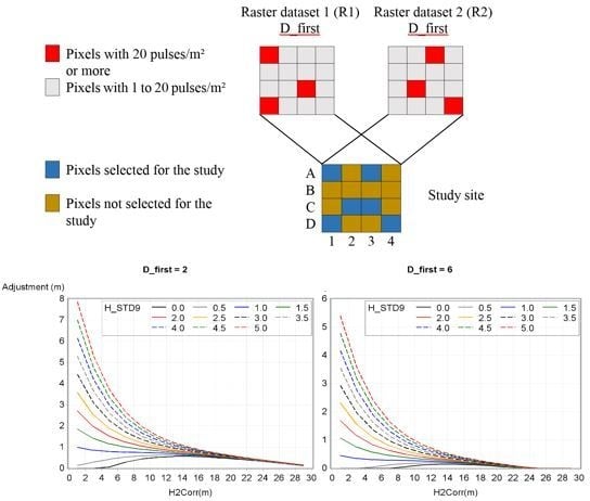
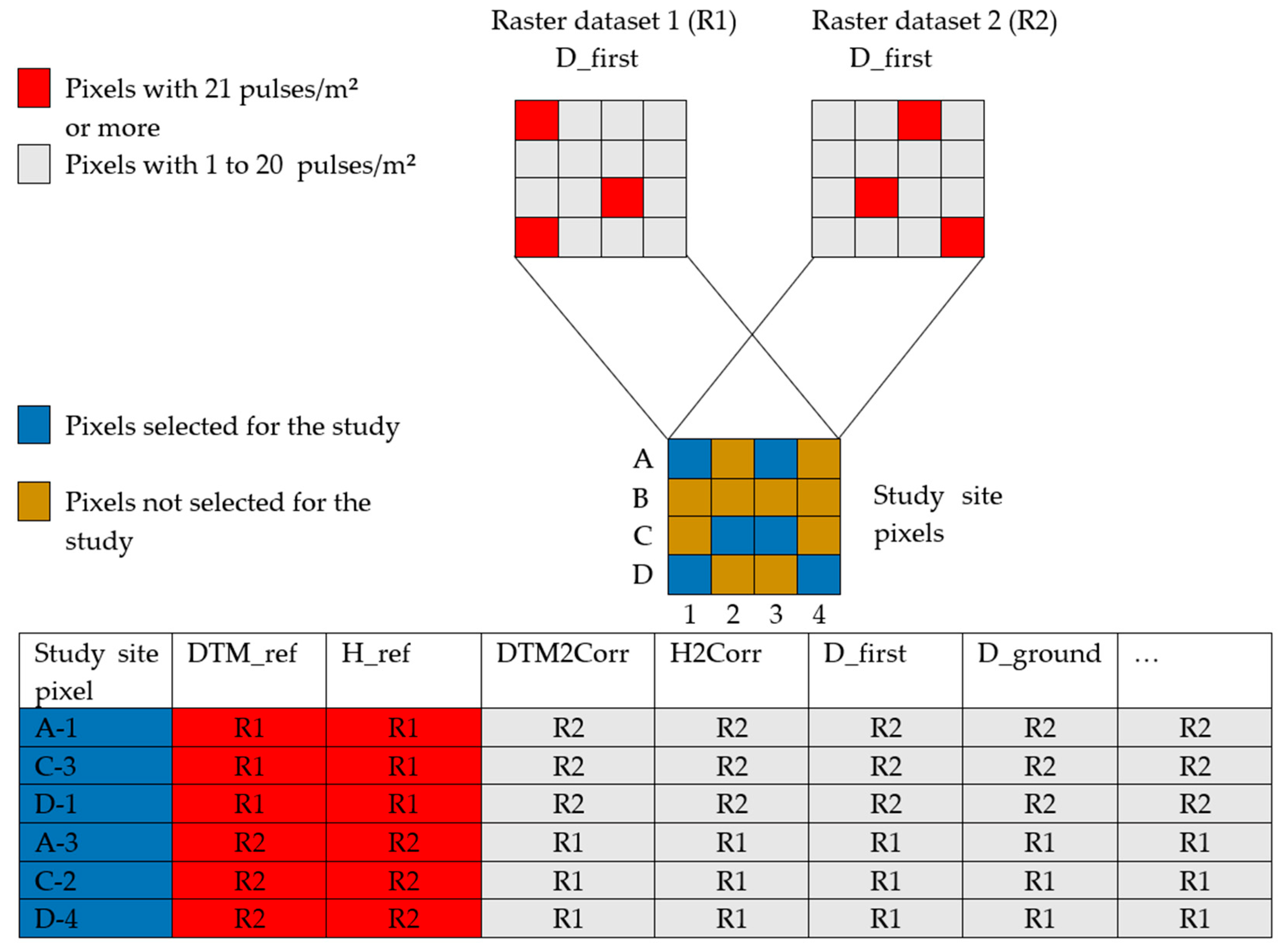
For each study site, all pixels originating from raster dataset 1 (R1) and having 21 pulses/m2 or more were selected. The DTM altitude (DTM_ref) and the maximum height (H_ref) in this pixel were calculated and were associated with the values originating from raster dataset 2 (R2), having D_first values between 1 to 20 pulses/m2. Values associated from R2 are DTM altitude (DTM2Corr), maximum height (H2Corr) and LiDAR variables detailed in Table 3. Thereafter, the opposite process was performed: DTM_ref and H_ref from pixels having 21 pulses/m2 or more of R2 were associated with corresponding values from R1 (Figure 3).
A database was thus generated where DTM_ref and H_ref enabled respectively, the evaluation of DTM and CHM biases. The DTM bias was calculated as DTM2Corr subtracted from DTM_ref and the CHM bias as H2Corr subtracted from H_ref. For graphic representations, a positive bias represented a height underestimation and a negative bias a height overestimation. The choice of pixels having 21 pulses/m2 or more, as reference value pixels, was based on Roussel et al. [10] who suggested that the maximal height had no significant bias for this type of pixels. Although the two surveys of each zone were not necessarily flown with the same sensor and the same acquisition parameters, it was assumed that these pixel values could be considered as the reference regardless of the sensor type and the parameters.
Some exclusions have been carried out in the two datasets (1 and 2) in order to minimize false biases due to anthropic or water level changes between the acquisitions. Thus, pixels located on water bodies, wetlands, agricultural areas, power lines, or gravel pits have been excluded. This filtering was conducted using Quebec’s existing ecoforest map [40]. Also, reference value pixels without ground returns were also excluded because the ground altitude value could be biased from neighbouring cells interpolation. Furthermore, pixels whose height was smaller than 0.5 m for one of the two datasets were also excluded in order to avoid adjusting bare soil areas (e.g., roads, recent cuts and gravel pits).
3. Modeling
Modeling the adjustments for DTM and CHM values consisted of three methodological steps that involved developing first a linear mixed model, followed by a non-linear model, and finally a non-linear mixed model. These steps were done for both DTM and CHM adjustment models with SAS (version 9.4, SAS Institute Inc., Cary, NC, USA).
3.1. Linear Mixed Model
For DTM and CHM adjustments, linear mixed regressions were performed to determine the independent variables contributing to the models. The independent variables tested were H2Corr (Table 1), LiDAR variables shown in Table 3, the sensor and the study sites. At this point, continuous variables were converted into classes to find the form of the relationship that reflects the effect of the variables. The variables D_first and D_ground were already in a class format as integer numbers. The number of classes per variable were respectively of 13, 8, 8, 8, 3, 9 for H2Corr, H_STD5, H_STD9, H_STD13, scan angles and slopes. We constructed models having a maximum of three independent variables including all interactions between them. At the beginning, a limit of three independent variables was imposed in order to have an easy to use model. To verify that more variables were not needed, residuals of the other variables were tested in each model. If residuals had revealed that more variables were needed, the maximum number of variables would have been adjusted.
Random effects among the 26 sites were estimated by testing the intercept coefficient using conditional and marginal predictions. First, conditional predictions were tested, taking into account the random effects of the study sites, and second, marginal predictions were tested by omitting these effects. For each linear mixed model, residuals were tested against all LiDAR acquisition variables to evaluate if variables that were not included in the fixed effects were explaining the residual variation.
Models tested the influence of D_first, D_ground, H2Corr and H_STD for the three neighborhood scales (H_STD5, H_STD9 and H_STD13). For the DTM adjustment models, there were no significant variables. The residuals were tested for sensors, terrain slopes, and scan angles. As a result, the methodology stopped here for the DTM and no specific adjustments were made.
For the canopy height adjustment models, the significant variables which were selected were H2Corr, D_first and H_STD9. An analysis of the residuals of these three independent variables indicated that it was appropriate to remove the pixels with terrain slopes greater than 45 degrees from the other analyses. Above these slope angles, the distribution of residuals showed a pattern indicating that this effect should be considered by the model. Even though the three neighbourhood scales for the height standard deviation were significant, the nine-cell neighbourhood was selected among the three based on R2 values. Moreover, marginal prediction was selected because the R2 barely increased when the study site was considered (mean difference of 1%). We concluded that in the case of this database, the study site (contractor, sensor, flight altitude and pulse frequency) did not influence height adjustment. Also, this led to a general model applicable to all the conditions tested in this study.
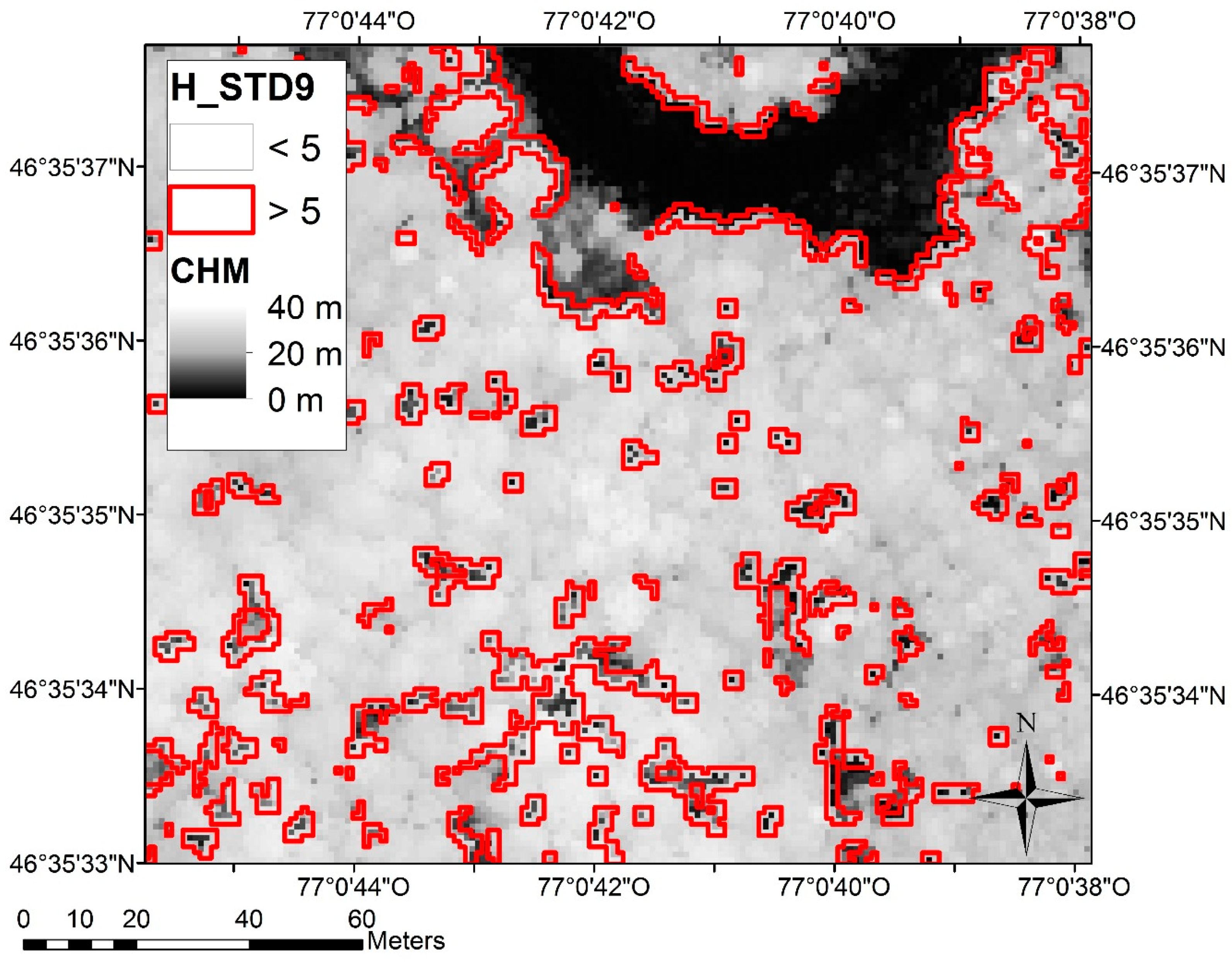
Based on visual observation, H_STD9 greater than five were recoded to five. This manipulation was applied because theses pixels represented forest canopy opening extremity (Figure 4). In these pixels, height was very variable depending on where pulses fell. As the adjustment increased with STD, unrealistic adjustments were predicted in these areas (8% of the pixels). A final linear mixed model was performed and an adjustment average was calculated for each combination of variable class (2080 combinations resulting from 20 D_first, 8 H_STD9 and 13 H2Corr classes). These averages were the inputs for the non-linear model.
3.2. Non-Linear Model
A non-linear model was used to find the shape of the equation. This model was weighted with the number of observations by class in order to give a more important weight for the more frequent values.
First, to visualize the equation form, one model was made for each H_STD9 and H2Corr class according to D_first. Thereby, the equation of the global form of the adjustments was simplified in the following way:
where α, β and ω were the model parameters.
Height adjustment = α + (β • D_firstω)
Second, the estimates of parameter β were visualized for each H2Corr class according to H_STD9. It was concluded that it was best represented by a linear equation:
β = β0 + β1 • H_STD9
Thereafter, estimates of β0 and β1 were visualized according to H2Corr. They respectively followed a simplification of the differential form of the Chapman-Richards equation and of an exponential curve.
Finally, the visualization of the two other parameters (ω and α) for each H2Corr classes according to H_STD9 simplified the selection of parameters during the modeling process.
Consequently, the non-linear model final equation was:
where:
where εjm was the error term of the jth pixel and for the mth study site.
Height adjustment = α + ((β0 + β1 • H_STD9) • D_firstω) + εjm
β0 = (β01 • e(−β02 • H2Corr) × (1 − e(−β02 • H2Corr))) − β00
β1 = β11 • e(−β12 • H2Corr)
3.3. Non-Linear Mixed Model
The final non-linear model equation was used in a non-linear mixed model to find the fixed coefficients with SAS® NLMIXED procedure. The random coefficient (δm) was added on the vertical intercept (α). The database included 3,263,872 pixels. For this model, 50% of the pixels from the original database of each site were randomly selected and used for the calibration.
3.4. Validation
The other 50% of the pixels were used for the validation. The CHM adjustment model was validated using this validation dataset. Thus, the model was applied on H2Corr and was compared with H_ref. The R2, the remaining bias on the corrected LiDAR height and the RMSE were then calculated.
4. Results
4.1. Selection of Resolution
By increasing the raster resolution from 1 to 2 m, the number of cells having 21 pulses/m2 or more decreased by 16.9 times and the number of cells without pulse only increased by 9.4 times. Based on these results, the 1 × 1 m resolution was chosen.
4.2. Shift in X, Y, Z
No planimetry shifts (X and Y) were detected using visual analyses across study sites. An altimetry shift higher than 0.2 m was detected over three study sites. These study sites were excluded, resulting in 26 study sites for the analysis.
4.3. Digital Terrain Model (DTM) Adjustment Model
Without any adjustments, the comparison of DTM_ref and DTM2Corr generated a RMSE of 0.25 m and a bias of −0.03 m.
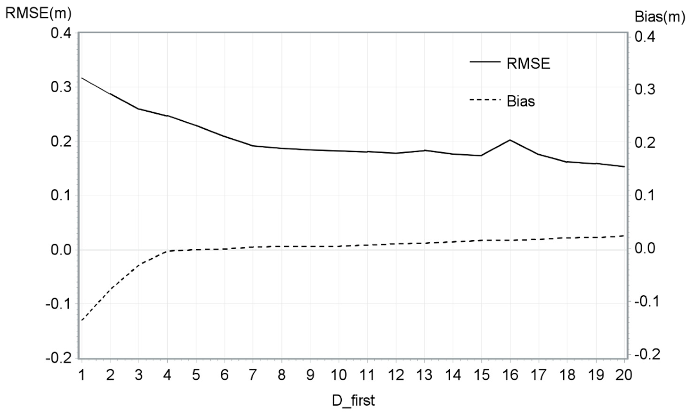
The best linear mixed model that was developed contained only one variable: D_first. The R2 of this model was 2%. In Table 4, all Pr > [t] are greater than 5%, which demonstrates that predictions are not significantly different from zero for all D_first. The RMSE and bias for D_first values are shown in Figure 5 to demonstrate the effect of D_first on accuracy statistics.
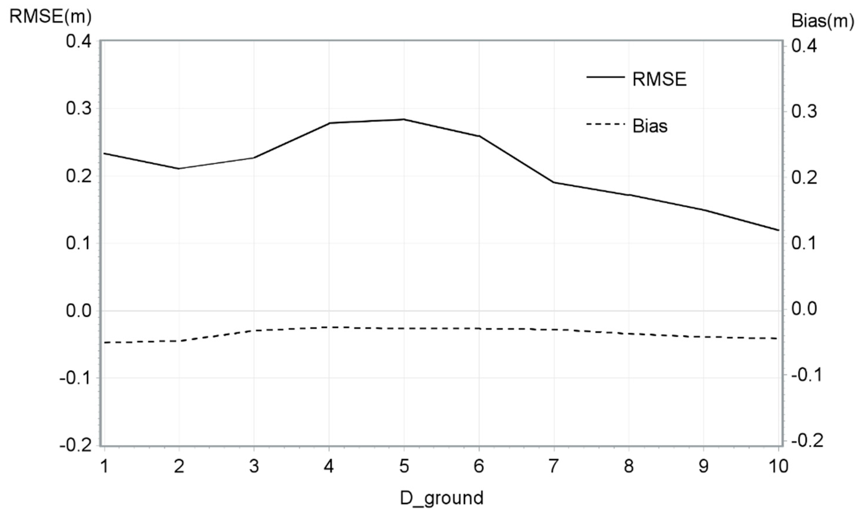
The second best model also included only one variable: D_ground. The R2 of this model was exceptionally low (0.05%). As for the previous model, Pr > [t] demonstrates that the model is not significantly different from zero. Bias and RMSE were calculated for D_ground values as shown in Figure 6. For this analysis, the D_ground values were between 1 and 10 ground pulses/m2 because insufficient observations were found above this value.
4.4. Canopy Height Model (CHM) Adjustment Model
The fixed coefficients of the non-linear mixed model are presented in Table 5 and the random coefficients according to study sites are found in Table 6. All acquisitions met Z precision requirements of ±0.50 m. All site random coefficients were lower than this value. The R2 of the final non-linear model was 22.8%.
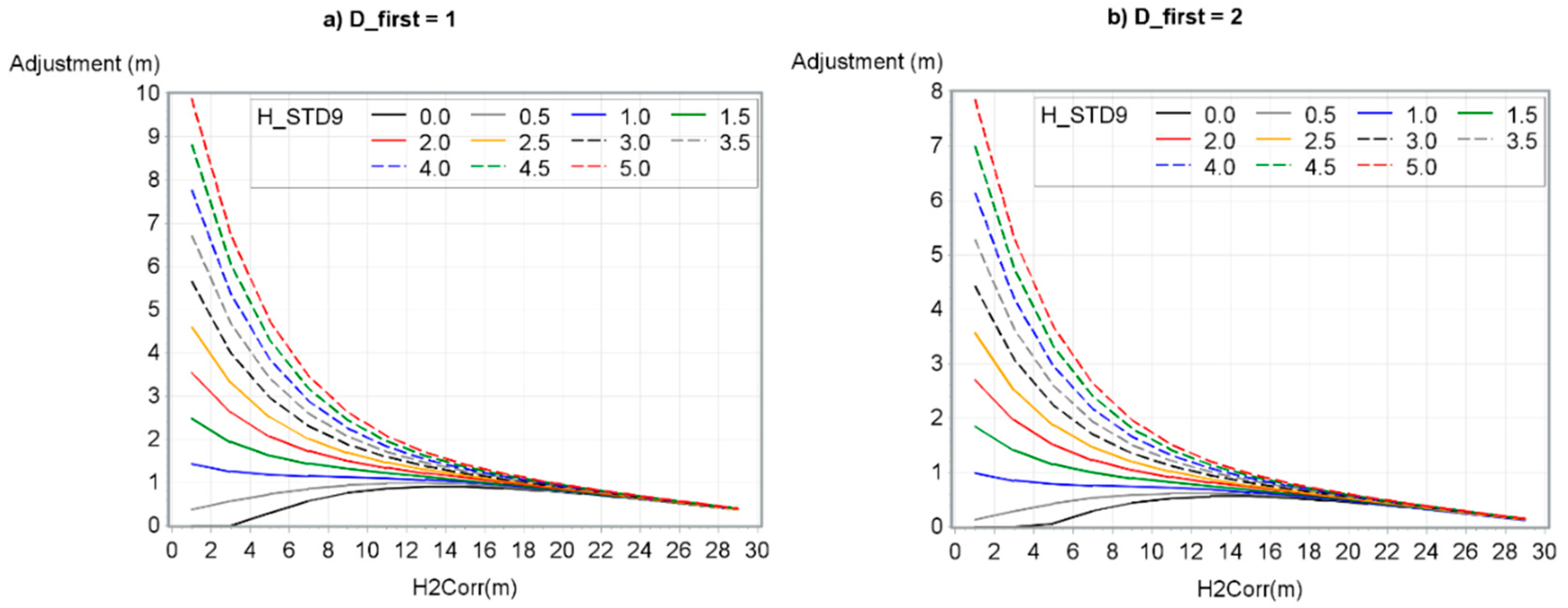
Figure 7 shows, for six D_first, the adjustment based on H2Corr and H_STD9 values.
Finally, H_STD9 is closely related to the forest cover type when compared with the ecoforest map [40] as shown in Table 7 which represented mean H_STD9 related to the mean H2Corr and forest cover type. As expected, coniferous stands had higher mean H_STD9 values than deciduous stands because of their conic shape and more irregular canopy.
4.5. Canopy Height Models Validation
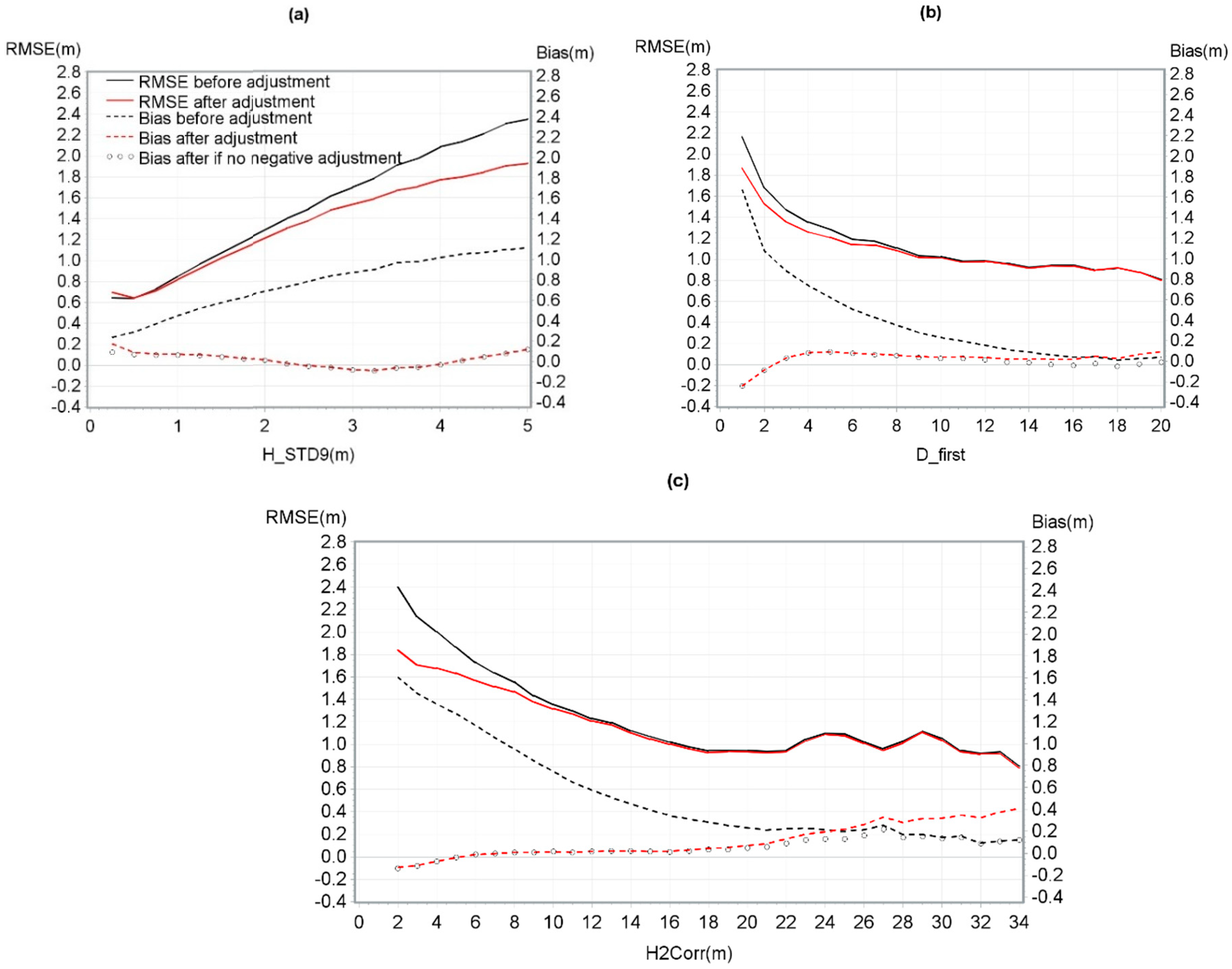
Based on the validation dataset, RMSE and bias were calculated before and after the regression. RMSE was 1.46 m and 1.30 m and bias was 0.70 m and 0.02 m respectively, before and after processing the regression. The mean bias and the RMSE were shown by H_STD9, D_first or H2Corr (Figure 8). The R2 between the H_ref and H2Corr was 92% (before the adjustment) versus 94% between H_ref and the corrected LiDAR height (after the adjustment).
5. Discussion
5.1. Digital Terrain Model (DTM) Adjustment Model
Both D_first (from 1 to 20 pulses/m2) and D_ground (from 1 to 10 ground pulses/m2) had no significant relationship with the DTM adjustment model. This was probably caused by the fact that the 1 × 1 m pixels preserved in the study contained at least one pulse. According to Watt et al. [22], a gradual decline in DTM accuracy can be detected from D_first between 0.7 and 1 pulses/m2. Our analysis concluded that for a DTM at a 1 × 1 m pixel size, D_first from 1 to 20 pulses/m2 has no significant difference on DTM altitude accuracy. However, it is important to note that this conclusion is only applicable at a 1 × 1 m pixel scale. Also, a LiDAR survey with a density of 1 pulses/m2 should be uniformly acquired at this pulse density to claim an accurate DTM (no pixel without pulse). In reality, for an acquisition aimed at 1 pulse/m2, some pixels have no pulse at all. These gaps should have influenced the DTM accuracy, but this study did not cover this aspect. Based on these results, we can conclude that a user should avoid obtaining pixels without pulses as much as possible to ensure an accurate 1 × 1 m DTM. In several cases, an average density of 2 to 3 pulses/m2 would be sufficient to minimize pixels without data. This was similar to Watt et al. [22], who recommended this density for accurate DTM.
In Figure 5 and Figure 6, the RSME is similar to the sensor accuracy (Table 2) and mean LiDAR Z error measured by Suàrez et al. [39]. This is also similar to the random DTM errors found by Hyyppä et al. [28]. In this study, authors demonstrated that DTM error is smaller than 0.2 m for most of the boreal forest conditions except for the slope where the error is greater.
The fact that significant adjustments are not necessary according to the parameters studied does not indicate that biases are inexistent in the DTM; this only shows that the parameters do not influence its global bias. Therefore, it is possible that within both low- and high-density surveys, biases remain locally in DTM and subsequently in CHM.
5.2. Canopy Height Model (CHM) Adjustment Model
The CHM adjustment model developed in this study was based on H2Corr, H_STD9 and D_first as dependent variables. Even though the R2 of the non-linear mixed model is low, 22.8%, the model is, however, significant and could be applicable over large areas. Some factors could explain this low R2: randomness in the distribution of LiDAR pulses, and the geographic shift between LiDAR datasets due to LiDAR precision. Nevertheless, the fact that the biases practically disappeared (0.70 m to 0.02 m) and that the RMSE was either stable or decreased slightly showed that the model gave accurate adjustments (Figure 8). These results were similar to those observed by Roussel et al. [10] who found an almost null bias and a reduced RMSE.
Resulting adjustments obtained from this model, as shown in Figure 7, presented noticeable observations. First, height adjustment decreased as both D_first and H2Corr increased while H_STD9 decreased. Second, H_STD9 had more impact on the results of the model for smaller H2Corr values. However, for low H_STD9 values (0 to 1 m), H2Corr values had a very small impact on the results of the model. Finally, the relationship between variables and resulting adjustments were similar to those observed by Roussel et al. [10] and Hirata [41]. Indeed, the adjustment followed an exponential curve, decreasing rapidly from D_first 1 to 10 pulses/m2 and more particularly from D_first 1 to 4 pulses/m2.
Furthermore, when the model gives a negative adjustment it is best not to adjust the height value. Figure 8 shows that not applying an adjustment instead of a negative adjustment reduced the bias in low H_STD9, high H2Corr, and high D_first. For D_first greater than 18, it prevented the bias from being greater after versus before adjustment.
Even though the R2 of the linear mixed model only increased by 1% when the study site was considered, Table 6 shows some differences amongst study sites. A link between the sensors or the flight parameters and the difference amongst the sites was not possible with the current dataset. The addition of study sites in the coming years could make it possible to study such relationships and reduce the effect of the study sites.
The results demonstrated that the model decreased CHM bias over large areas. However, the user must take into account several factors. First, even though the equation gives a height adjustment for 1 × 1 m pixels, it is important to take into account that it gives an average corrected height value and not an exact height value per pixel. Second, it was important not to apply the model on steep slopes (more than 45 degrees), water bodies, wetlands, agricultural areas, power lines and gravel pits because these areas were excluded from the model. Third, this model was only applicable on discrete return LiDAR sensors and in leaf-on conditions. Finally, despite these aspects that the user has to keep in mind, the study demonstrated that the model could be applied to a very large range of ecological conditions in the Canadian boreal shield ecozone and to a wide range of LiDAR acquisition parameters.
6. Conclusions
The goals of this study were to propose an adjustment model to correct a DTM bias, and ultimately, to propose an adjustment model to correct CHM bias for a wide range of terrain and acquisition conditions. According to our database and the chosen 1 × 1 m resolution, no variable significantly influenced the DTM correction model and consequently, no models was calculated for DTM. However, three variables were selected for the final CHM adjustment model based on the database in this study and the variables studied: H2Corr, D_first and H_STD9. This model resulted a reduction of the mean bias from 0.70 m to 0.02 m. Also, several notable observations emerged from this study. Among them, the height adjustment decreased as both D_first and H2Corr increased and H_STD9 decreased. The H_STD9 variable had more impact on the adjustments of model for smaller H2Corr values.
This study was a first attempt to correct LiDAR heights according to a wide range of conditions: 6 sensors studied, diverse angles or pulse densities and study sites covering 3 500 km2 and located on different ecological conditions. Also, results obtained support most of height underestimation studies in the literature. The CHM underestimation correction is a preliminary step to several uses of the CHM such as volume calculation, forest growth models or multi-temporal analysis. For example, before modeling growth with multi-temporal LiDAR data, the underestimation bias on each CHM should be removed; the present work can thus be used in this context.
Finally, its application on various additional data sets in the near future may result in an improvement of models, and may provide better analyses of sensor effects.
Author Contributions
Conceptualization, A.L., J.B., M.-S.F., M.R.; Methodology, A.L., M.-S.F.; Analysis, M.-S.F., M.R.; Writing, M.-S.F.; Review & Editing, A.L., J.B., M.-S.F., M.R.
Funding
The first author received a scholarship from the Fonds de recherche québécois sur la nature et les technologies (FRQNT).
Acknowledgments
We would like to thank the MFFP for providing LiDAR data and Marie R. Coyea and Anne Théodorescu for the English revision. We would also thanks anonymous reviewers for their insightful comments.
Conflicts of Interest
The authors declare no conflicts of interest.
Appendix A

Table A1.
Metadata of the 26 study sites used for the study.
| Study Site/Dataset 1-Dataset 2 | Dataset 1 | Dataset 2 | Species Composition Based on the Quebec Ecoforest Map [40] (Max 4 Main Species *) | ||||
|---|---|---|---|---|---|---|---|
| Sensor ** | Altitude | Frequency | Sensor ** | Altitude | Frequency | ||
| 1/A-B | OPGE | 650 | 125 | LEHP | 1200 | 190 | BF, BS, WB, TA |
| 2/C-D | OPGE | 750 | 125 | LEHP | 1350 | 385 | BS, BF, WB, JP |
| 3/C-E | OPGE | 750 | 125 | OPGE | 750 | 125 | BF, WB, EN, BJ |
| 4/E-C | OPGE | 750 | 125 | OPGE | 750 | 125 | BF, WB, EN, BJ |
| 5/E-F | OPGE | 750 | 125 | LEHP | 850 | 250 | BS, BF, WB, TA |
| 6/I-J | OPGE | 650 | 125 | LEHP | 1375 | 385 | BF, YB, SM |
| 7/K-L | OPGE | 950 | 100 | O3100 | 1250 | 70 | BS, T, WB, BF |
| 8/K-M | OPGE | 950 | 100 | OPGE | 1000 | 100 | T, WP, JP |
| 9/B-A | LEHP | 1200 | 190 | OPGE | 650 | 125 | BF, BS, WB, TA |
| 10/D-C | LEHP | 1350 | 385 | OPGE | 750 | 125 | BS, BF, WB, JP |
| 11/F-G | LEHP | 850 | 250 | LEHP | 850 | 250 | SM, RM, TA, YB |
| 12/G-F | LEHP | 850–1600 | 250–320 | LEHP | 850 | 250 | SM, RM, TA, YB |
| 13/G-H | LEHP | 850 | 250 | RL680 | 700 | 300 | WP, RM, TA, SM |
| 14/J-I | LEHP | 1375 | 385 | OPGE | 650 | 125 | BF, YB, SM |
| 15/O-N | LEHP | 1936 | 385 | OPGA | 1300 | 250 | BS, WS, WB, JP |
| 16/P-N | LEHP | 800–1600 | 175–330 | OPGA | 1300 | 250 | WB, BS, WS, YB |
| 17/O-P | LEHP | 1936 | 565 | LEHP | 800–1600 | 175–330 | BS, JP, TA, WB |
| 18/P-O | LEHP | 800–1600 | 175–330 | LEHP | 1936 | 565 | BS, JP, TA, WB |
| 19/H-G | RL680 | 700 | 300 | LEHP | 850 | 250 | WP, RM, TA, SM |
| 20/Q-R | RL680 | 900 | 80 | OPGE | 800 | 142 | JP, BS, TA |
| 21/S-W | RL680 | 850 | 240 | RL780 | 850 | 400 | BS, JP, T |
| 22/S-X | RL680 | 1000 | 240 | RL780 | 850 | 400 | BS, BF, WB, TA |
| 23/U-Y | RL680 | 900 | 240 | RL780 | 850 | 400 | YB, BF, WB, TA |
| 24/V-Z | OPGA | 1550 | 300 | RL780 | 850 | 400 | RM, YB, SM, BF |
| 25/N-O | OPGA | 1300 | 250 | LEHP | 1936 | 565 | BS, WS, WB, JP |
| 26/N-P | OPGA | 1300 | 250 | LEHP | 800–1600 | 175–330 | WB, BS, WS, YB |
* Black spruce = BS, White birch = WB, Balsam fir = BF, Trembling aspen = TA, Jack pine = JP, Sugar maple = SM, Yellow birch = YB, Tamarack = T, White pine = WP, White spruce = WS, Red maple = RM. ** Riegl LMS-Q680i = RL680, Optech ALTM Gemini = OPGE, Leica ALS70-HP = LEHP, Optech ALTM Galaxy = OPGA, Riegl LMS-Q780 = RL780, Optech 3100EA = O3100.
References
- Moran, C.J.; Rowell, E.M.; Seielstad, C.A. A data-driven framework to identify and compare forest structure classes using LiDAR. Remote Sens. Environ. 2018, 211, 154–166. [Google Scholar] [CrossRef]
- Torresan, C.; Corona, P.; Scrinzi, G.; Marsal, J. Using classification trees to predict forest structure types from LiDAR data. Ann. For. Sci. 2016, 59, 281–298. [Google Scholar] [CrossRef]
- Tompalski, P.; Coops, N.C.; White, J.C.; Wulder, M.A. Simulating the impacts of error in species and height upon tree volume derived from airborne laser scanning data. For. Ecol. Manag. 2014, 327, 167–177. [Google Scholar] [CrossRef]
- Ruiz, L.; Hermosilla, T.; Mauro, F.; Godino, M. Analysis of the Influence of Plot Size and LiDAR Density on Forest Structure Attribute Estimates. Forests 2014, 5, 936–951. [Google Scholar] [Green Version]
- Yoga, S.; Bégin, J.; Daigle, G.; Riopel, M.; St-Onge, B. A Generalized Lidar-Based Model for Predicting the Merchantable Volume of Balsam Fir of Sites Located along a Bioclimatic Gradient in Quebec, Canada. Forests 2018, 9, 166. [Google Scholar] [CrossRef]
- Estornell, J.; Ruiz, L.; Velázquez-Martí, B.; Fernández-Sarría, A. Estimation of shrub biomass by airborne LiDAR data in small forest stands. For. Ecol. Manag. 2011, 262, 1697–1703. [Google Scholar] [CrossRef] [Green Version]
- Gleason, J.C.; Im, J. Forest biomass estimation from airborne LiDAR data using machine learning approaches. Remote Sens. Environ. 2012, 125, 80–91. [Google Scholar] [CrossRef]
- Gaveau, L.A.D.; Hill, R.A. Quantifying canopy height underestimation by laser pulse penetration in small-footprint airborne laser scanning data. Can. J. Remote Sens. 2003, 29, 650–657. [Google Scholar] [CrossRef]
- Disney, M.I.; Kalogirou, V.; Lewis, P.; Prieto-Blanco, A.; Hancock, S.; Pfeifer, M. Simulating the impact of discrete-return lidar system and survey characteristics over young conifer and broadleaf forests. Remote Sens. Environ. 2010, 114, 1546–1560. [Google Scholar] [CrossRef]
- Roussel, J.-R.; Caspersen, J.; Béland, M.; Thomas, S.; Achim, A. Removing bias from LiDAR-based estimates of canopy height: Accounting for the effects of pulse density and footprint size. Remote Sens. Environ. 2017, 198, 1–16. [Google Scholar] [CrossRef]
- Isenburg, M. Density and Spacing of LiDAR. Available online: https:/rapidlasso.com/2014/03/20/density-and-spacing-of-lidar/ (accessed on 5 June 2018).
- Liu, J.K.; Skidmore, A.; Jones, S.; Wang, T.; Heurich, M.; Zhu, X.; Shi, Y. Large off-nadir scan angle of airborne LiDAR can severely affect the estimates of forest structure metrics. ISPRS J. Photogramm. J. 2018, 136, 13–25. [Google Scholar] [CrossRef]
- Holmgren, J.; Nilsson, M.; Olsson, H. Simulating the effects of lidar scanning anglefor estimation of mean tree height and canopy closure, Québec. Can. J. Remote Sens. 2003, 29, 623–632. [Google Scholar] [CrossRef]
- Montaghi, A. Effect of scanning angle on vegetation metrics derived from a nationwide Airborne Laser Scanning acquisition. Can. J. Remote Sens. 2014, 39, 152–173. [Google Scholar] [CrossRef]
- Hopkinson, C. The influence of flying altitude, beam divergence, and pulse repetition frequency on laser pulse return intensity and canopy frequency distribution. Can. J. Remote Sens. 2007, 33, 312–324. [Google Scholar] [CrossRef]
- St-Onge, B. Estimating individual tree heights of the boreal forest using airborne laser altimetry and digital videography. Arch. Photogramm. Remote Sens. 1999, 32, 179–184. [Google Scholar]
- Sibona, E.; Vitali, A.; Meloni, F.; Caffo, L.; Dotta, A.; Lingua, E.; Motta, R.; Garbarino, M. Direct Measurement of Tree Height Provides Different Results on the Assessment of LiDAR Accuracy. Forests 2017, 8, 7. [Google Scholar] [CrossRef]
- Gatziolis, D.; Fried, J.; Monleon, V. Challenges to estimating tree height via LiDAR in closed-canopy forest: A parable from western Oregon. For. Sci. 2010, 56, 139–155. [Google Scholar]
- Tinkham, T.W.; Smith, M.S.; Hoffman, A.C.; Hudak, A.T.; Falkowski, M.J.; Swanson, M.E.; Gessler, E.P. Investigating the influence of LiDAR ground surface errors on the utility of derived forest inventories. Can. J. For. Res. 2012, 42, 413–422. [Google Scholar] [CrossRef]
- Takeda, H. Ground surface estimation in dense forest. ISPRS Arch. 2004, 35, 1016–1023. [Google Scholar]
- Leckie, D.; Gougeon, F.; Hill, D.; Quinn, R.; Armstrong, L.; Shreenan, R. Combined high-density lidar and multispectral imagery for individual tree crown analysis. Can. J. Remote Sens. 2003, 29, 633–649. [Google Scholar] [CrossRef] [Green Version]
- Watt, M.S.; Meredith, A.; Watt, P.; Aaron, G. The influence of LiDAR pulse density on the precision of inventory metrics in young unthinned Douglas-fir stands during initial and subsequent LiDAR acquisitions. N. Z. J. For. Sci. 2014, 44, 18. [Google Scholar] [CrossRef] [Green Version]
- Treitz, P.; Lim, K.; Woods, M.; Pitt, D.; Nesbitt, D.; Etheridge, D. LiDAR sampling density for forest resource inventories in Ontario, Canada. Remote Sens. 2012, 4, 380–848. [Google Scholar] [CrossRef]
- Bater, C.W.; Wulder, M.A.; Coops, N.C.; Nelson, R.F.; Hilker, T.; Næsset, E. Stability of sample-based scanning-lidar-derived vegetation metrics for forest monitoring. IEEE Trans. Geosci. Remote Sens. 2011, 49, 2385–2392. [Google Scholar] [CrossRef]
- Lefsky, M.; Cohen, W.; Parker, G.; Harding, D. Lidar remote sensing for ecosystem studies. Bioscience 2002, 52, 19–30. [Google Scholar] [CrossRef]
- Naesset, E.; Okland, T. Estimating tree height and tree crown properties using airborne scanning laser in a boreal nature reserve. Remote Sens. Environ. 2002, 79, 105–115. [Google Scholar] [CrossRef]
- Yu, X.; Hyyppä, J.; Hyyppä, H.; Maltamo, M. Effects of flight altitude on tree height estimation using airborne laser scanning. Arch. Photogramm. Remote Sens. Spat. Inf. Sci. 2004, 36, 96–101. [Google Scholar]
- Hyyppä, J.; Hyyppä, H.; Leckie, D.F.; Gougeon, X.Y.; Maltamo, M. Review of methods of small-footprint airborne laser scanning for extracting forest inventory data in boreal forests. Int. J. Remote Sens. 2008, 29, 1339–1366. [Google Scholar] [CrossRef]
- MDDELCC. Normales Climatiques du Québec 1981–2010. Available online: http://www.mddelcc.gouv.qc.ca/climat/normales/index.asp (accessed on 5 June 2018).
- AAFC. Effective Growing Degree Days in Quebec. Available online: http://www.agr.gc.ca/eng/science-and-innovation/agricultural-practices/agriculture-and-climate/future-outlook/climate-change-scenarios/effective-growing-degree-days-in=quebec/?id=1363104035947 (accessed on 5 June 2018).
- Schneider, F.D.; Leiterer, R.; Morsdorf, F.; Gastellu-Etchegorry, J.-P.; Lauret, N.; Pfeifer, N.; Schaepman, E.M. Simulating imaging spectrometer data: 3D forest modeling based on LiDAR and in situ data. Remote Sens. Environ. 2014, 152, 235–250. [Google Scholar] [CrossRef]
- Optech Incorporated. Gemini ALTM. Available online: http://airsensing.com/wp-content/uploads/2014/11/Airborne_Gemini.pdf (accessed on 25 March 2019).
- Leica Geosystems AG. Leica ALS70-CM, City Mapping Airborne LIDAR, Product Specifications. Available online: https://w3.leica-geosystems.com/downloads123/zz/airborne/ALS70/product-specification/ALS70CM_ProductSpecs_en.pdf (accessed on 25 March 2019).
- Teledyne Optech Incorporated. Optech ALTM Galaxy, Airborne LiDAR System. Available online: https://geo-matching.com/uploads/default/m/i/migratione8z2fw.pdf (accessed on 25 March 2019).
- Colucci, R.R.; Žebre, M. Late Holocene evolution of glaciers in the southeastern Alps. J. Maps 2016, 12, 289–299. [Google Scholar] [CrossRef] [Green Version]
- Kaartinen, H.; Hyyppä, J.; Yu, X.; Vastaranta, M.; Hyyppä, H.; Kukko, A.; Holopainen, M.; Heipke, C.; Hirschmugl, M.; Morsdorf, F.; et al. An International Comparison of Individual Tree Detection and Extraction Using Airborne Laser Scanning. Remote Sens. 2012, 4, 950–974. [Google Scholar] [CrossRef] [Green Version]
- Wallace, L.; Lucieer, A.; Watson, C.S. Evaluating tree detection and segmentation routines on very high resolution UAV lidar data. IEEE Trans. Geosci. Remote Sens. 2014, 52, 7619–7628. [Google Scholar] [CrossRef]
- Vepakomma, U.; St-Onge, B.; Kneeshaw, D. Spatially explicit characterization of boreal forest gap dynamics using multi-temporal lidar data. Remote Sens. Environ. 2008, 112, 2326–2340. [Google Scholar] [CrossRef]
- Suárez, C.J.; Ontiveros, C.; Smith, S.; Snape, S. Use of airborne LiDAR and aerial photography in the estimation of individual tree heights in forestry. Comput. Geosci. 2005, 31, 253–262. [Google Scholar] [CrossRef]
- MFFP. Inventaire écoforestier. Available online: https://mffp.gouv.qc.ca/les/forets /amenagement-durable-forets/inventaire-ecoforestier/ (accessed on 26 June 2018).
- Hirata, Y. The effects of footprint size and sampling density in Airborne Laser Scanning to extract individual trees in mountainous terrain. Arch. Photogramm. Remote. Sens. Spat. Inf. Sci. 2004, 36, 102–107. [Google Scholar]
Figure 1.
Location of study sites in Quebec, Canada.

Figure 2.
Pixel studied neighborhood for the variable H_STD5, H_STD9 and H_STD13.

Figure 3.
Schema for the generation of the database.

Figure 4.
H_STD9 values of more than five for a low density LiDAR survey overlaid on a CHM.

Figure 5.
RMSE and mean bias of the DTM model by D_first.

Figure 6.
RMSE and mean bias of the DTM model by D_ground.

Figure 7.
CHM adjustment according to H2Corr, H_STD9 and D_first. (a) D_first = 1, (b) D_first = 2, (c) D_first = 4, (d) D_first = 6, (e) D_first = 10 and (f) D_first = 15.
Figure 7.
CHM adjustment according to H2Corr, H_STD9 and D_first. (a) D_first = 1, (b) D_first = 2, (c) D_first = 4, (d) D_first = 6, (e) D_first = 10 and (f) D_first = 15.


Figure 8.
RMSE and mean bias of the CHM model based on (a) H_STD9, (b) D_first, and (c) H2Corr.

Table 1.
Main forest characteristics.
| Forest Characteristics | Data | ||
|---|---|---|---|
| Mean annual temperature | 0.1 °C to 5.1 °C [29] | ||
| Mean annual precipitation | 860 to 1135 mm [29] | ||
| Forest cover | Deciduous | 25% | |
| Mixed | 46% | ||
| Coniferous | 29% | ||
| Growing degree days (>5 °C) | Mean minimum | 900 [30] | |
| Mean maximum | 1400 [30] | ||
| Range | Mean | Standard deviation | |
| Height (m) | 0–35 | 11.38 | 5.71 |
| Crown closure (%) | 0–100 | 72.2 | 19.1 |
Table 2.
LiDAR acquisition characteristics by sensor.
| Sensors | ||||||
|---|---|---|---|---|---|---|
| Characteristics | Riegl LMS-Q680i | Optech ALTM Gemini | Leica ALS70-HP | Optech ALTM Galaxy | Riegl LMS-Q780 | Optech 3100EA |
| Pulse repetition frequency (kHz) | 80–300 | 100–142 | 175–565 | 200–250 | 400 | 70 |
| Ground flight altitude (m) | 700–1000 | 650–1200 | 800–1600 | 1300–1550 | 400 | 1250 |
| Z accuracy (m) | <0.15 [31] | 0.05–0.30 [32] | 0.07–0.16 [33] | 0.03–0.20 [34] | <0.15 [35] | <0.15 [17] |
Table 3.
LiDAR acquisition variables calculated.
| LiDAR Variables | Description | Unit | Values | Algorithm Used | ||
|---|---|---|---|---|---|---|
| Range | Mean | Standard Deviation | ||||
| First return density (D_first) | Number of first return or number of pulses per m2 | Pulses/m2 | 1–20 | 4.98 | 3.81 | LAStools – Lasgrid |
| Ground point density (D_ground) | Number of ground point per m2 | Pulses/m2 | 0–20 | 0.76 | 1.31 | LAStools – Lasground |
| Scan angles | Minimum per m2 | Degrees | 0–34 | 7.29 | 4.93 | LAStools – Lasgrid |
| Mean per m2 | Degrees | 0–34 | 9.15 | 5.52 | LAStools – Lasgrid | |
| Maximum per m2 | Degrees | 0–38 | 10.82 | 6.83 | LAStools – Lasgrid | |
| Terrain slopes | Mean slopes per m2 | Degrees | 0–84 | 8.09 | 7.71 | LAStools – Las2dem |
| Maximum height standard deviation for 5 neighbourhood cells (H_STD5) | As described in Figure 2 | Meters | 0–26.65 | 1.95 | 1.45 | ESRI focal statistics of Spatial analyst |
| Maximum height standard deviation for 9 neighbourhood cells (H_STD9) | As described in Figure 2 | Meters | 0–25.66 | 2.73 | 1.54 | ESRI focal statistics of Spatial analyst |
| Maximum height standard deviation for 13 neighbourhood cells (H_STD13) | As described in Figure 2 | Meters | 0–26.50 | 2.37 | 1.51 | ESRI focal statistics of Spatial analyst |
Table 4.
Marginal predicted means (m) of D_first effect on DTM adjustment linear mixed model.
| D_first | Estimate | Pr > [t] | D_first | Estimate | Pr > [t] |
|---|---|---|---|---|---|
| 1 | −0.045 | 0.0957 | 11 | −0.016 | 0.5599 |
| 2 | −0.040 | 0.1414 | 12 | −0.013 | 0.6391 |
| 3 | −0.036 | 0.1899 | 13 | −0.012 | 0.6542 |
| 4 | −0.035 | 0.2009 | 14 | −0.011 | 0.6800 |
| 5 | −0.033 | 0.2220 | 15 | −0.011 | 0.6969 |
| 6 | −0.028 | 0.3012 | 16 | −0.012 | 0.6459 |
| 7 | −0.026 | 0.3377 | 17 | −0.015 | 0.5820 |
| 8 | −0.023 | 0.3882 | 18 | −0.018 | 0.4987 |
| 9 | −0.021 | 0.4334 | 19 | −0.023 | 0.3921 |
| 10 | −0.019 | 0.4806 | 20 | −0.029 | 0.2940 |
Table 5.
Fixed coefficients of height adjustment model for CHM (Equations (3)–(5)).
| Coefficients | Value | p-Value |
|---|---|---|
| α | −0.9142 | <0.0001 |
| β00 | 0.1196 | <0.0001 |
| β01 | 7.7737 | <0.0001 |
| β02 | 0.0496 | <0.0001 |
| β11 | 2.6155 | <0.0001 |
| β12 | 0.2160 | <0.0001 |
| ω | −0.3021 | <0.0001 |
Table 6.
Random coefficients (δm) of height adjustment model for CHM.
| Study Sites * | Value | p-Value | Study Sites | Value | p-Value |
|---|---|---|---|---|---|
| 1 | 0.07 | 0.0405 | 14 | −0.08 | 0.0299 |
| 2 | 0.00 | 0.9338 | 15 | 0.27 | <0.0001 |
| 3 | 0.25 | <0.0001 | 16 | 0.08 | 0.0371 |
| 4 | 0.24 | <0.0001 | 17 | −0.01 | 0.7966 |
| 5 | 0.27 | <0.0001 | 18 | −0.08 | 0.0389 |
| 6 | 0.09 | 0.0202 | 19 | 0.10 | 0.0073 |
| 7 | −0.09 | 0.0868 | 20 | −0.33 | < 0.0001 |
| 8 | 0.05 | 0.1967 | 21 | −0.16 | 0.0006 |
| 9 | −0.12 | 0.0107 | 22 | −0.17 | 0.0006 |
| 10 | −0.19 | <0.0001 | 23 | −0.07 | 0.0961 |
| 11 | 0.22 | <0.0001 | 24 | −0.10 | 0.0105 |
| 12 | 0.17 | 0.0009 | 25 | −0.40 | <0.0001 |
| 13 | 0.02 | 0.6196 | 26 | −0.04 | 0.3022 |
* Study sites are described in more detail for species and sensors in Appendix A.
Table 7.
Mean H_STD9 according to the H2Corr and the forest cover.
| Forest Cover Type | |||
|---|---|---|---|
| Deciduous | Mixed | Coniferous | |
| Mean H2Corr (m) | Mean H_STD (m) | ||
| <12 | 1.27 | 1.50 | 2.10 |
| 22 to 12 | 1.69 | 1.99 | 2.45 |
| >22 | 1.90 | 2.57 | 3.09 |
© 2019 by the authors. Licensee MDPI, Basel, Switzerland. This article is an open access article distributed under the terms and conditions of the Creative Commons Attribution (CC BY) license (http://creativecommons.org/licenses/by/4.0/).
Share and Cite
MDPI and ACS Style
Fradette, M.-S.; Leboeuf, A.; Riopel, M.; Bégin, J. Method to Reduce the Bias on Digital Terrain Model and Canopy Height Model from LiDAR Data. Remote Sens. 2019, 11, 863. https://0-doi-org.brum.beds.ac.uk/10.3390/rs11070863
AMA Style
Fradette M-S, Leboeuf A, Riopel M, Bégin J. Method to Reduce the Bias on Digital Terrain Model and Canopy Height Model from LiDAR Data. Remote Sensing. 2019; 11(7):863. https://0-doi-org.brum.beds.ac.uk/10.3390/rs11070863
Chicago/Turabian StyleFradette, Marie-Soleil, Antoine Leboeuf, Martin Riopel, and Jean Bégin. 2019. "Method to Reduce the Bias on Digital Terrain Model and Canopy Height Model from LiDAR Data" Remote Sensing 11, no. 7: 863. https://0-doi-org.brum.beds.ac.uk/10.3390/rs11070863
Note that from the first issue of 2016, this journal uses article numbers instead of page numbers. See further details here.