Multispectral Contrast of Archaeological Features: A Quantitative Evaluation


1
Institute for Archaeological and Monumental Heritage (IBAM), National Research Council (CNR), C.da Santa Loja, 85050 Tito Scalo (PZ), Italy
2
Institute of Methodologies for Environmental Analysis (IMAA), National Research Council (CNR), C.da Santa Loja, 85050 Tito Scalo (PZ), Italy
3
Department of Geography, Durham University, Lower Mountjoy, South Road, Durham, DH1 3LE, UK
*
Author to whom correspondence should be addressed.
Remote Sens. 2019, 11(8), 913; https://0-doi-org.brum.beds.ac.uk/10.3390/rs11080913
Submission received: 22 February 2019
/
Revised: 25 March 2019
/
Accepted: 8 April 2019
/
Published: 15 April 2019
(This article belongs to the Special Issue 2nd Edition Advances in Remote Sensing for Archaeological Heritage)
Abstract
:This study provides an evaluation of spectral responses of hollow ways in Upper Mesopotamia. Hollow ways were used for the transportation of animals, carts, and other moving agents for centuries. The aim is to show how the success of spectral indices varies in describing topologically simple features even in a seemingly homogeneous geographic unit. The variation is further highlighted under the changing precipitation regime. The methodology begins with an exploration of the relationship between the date of a multispectral scene and the visibility of hollow ways. The next step is to evaluate the impact of rainfall levels on numerous indices and to quantify spectral contrast. The contrast between a hollow way and its background is evaluated with Welch’s t-test and the association between precipitation regime and spectral responses of hollow ways are investigated with Correspondence Analysis and Fisher’s test. Results highlight an intrinsic relationship between the precipitation regime and the ways in which archaeological features reflects and/or emits electromagnetic energy. Next, the categorization of spectral indices based on different rainfall levels can be used as a guidance in future studies. Finally, the study suggests contrast becomes an even more fruitful concept as one moves from the spatial domain to the spectral domain.
1. Introduction
In remote sensing, the detection of an archaeological feature within its surrounding matrix depends on the level of contrast [1]; a target is easier to decipher—both visually and computationally—when it has higher contrast. Within the context of satellite remote sensing, contrast is the difference between the electromagnetic energy emitted and/or reflected from a feature (or its proxy) and the background energy. The level of difference as registered by the sensor determines whether the feature mapping and analysis will be successful.
Contrast is an underlying concept of all remote mapping projects. In particular, the increasing access to Very High Resolution (VHR) satellite imagery (with sub-meter resolutions in panchromatic bands) and the widespread use of online imagery viewing platforms make it easier to manually or (semi-)automatically detect potential targets [2]. While doing so, researchers tend to focus mainly on spatial manifestations of spectral contrast: that is, the separation boundary between two internally homogeneous spectral sets. Yet, spectral data in and of themselves also contain useful information aside from location and shape.
To date, a wide range of spectral data analyses have been performed in order to identify the relation between vegetation classes and human occupation patterns [3], solve the spectral mixture problem [4], or investigate human-environment relations [5]. In particular, detection and documentation of archaeological features have been an important research domain [6,7,8]. However, aside from a few notable examples [9,10,11] the temporal conditions of spaceborne spectral data and how archaeological features react spectrally to these conditions (especially for changing climatic conditions) have not fully attracted the attention of archaeologists.
Satellite remote sensing analysis is most successful when the electromagnetic energy emitted and/or reflected from an archaeological feature is directly recorded by the sensor (i.e., direct contrast). However, proxy data may be used if direct detection is not possible, such as when the feature is buried [1]. In fact, this approach has been extensively discussed in the literature on aerial remote sensing [12,13]. For instance, wall foundations, ancient water channels, and compacted road surfaces can be detected by proxy by studying the vegetation growth both above and around them. In another example, a buried structure replaces the soil and limits the amount of nutrients available to the vegetation above it. Thus, the biomass above buried archaeological features becomes less healthy in comparison to vegetation with access to deeper soils. Likewise, differential deposition (e.g., an ancient ditch later in-filled with loose topsoil) may create variations in moisture-retention capacity such that the buried feature may be still visible as soil mark proxies. Exploiting these relations, researchers can use multispectral analysis of vegetation and/or bare soils in order to document both buried and unburied archaeological features [14,15].
Vegetation and soil characteristics and their energy reflections on the electromagnetic spectrum are variable. For instance, optimal conditions for measuring agricultural crop characteristics via satellite sensors are distorted when local producers variably observe and react to seasonal climatic variations, and this may result in canopy differences even at short distances. Also, even if the biomass is compatible, different crop-management strategies—such as non-uniform access to irrigation, manuring, weed control, row spacing, and field orientation—have an impact on the relations between vegetation and how it is measured with a multispectral satellite sensor [16,17,18]. To normalize for such external factors, remote sensing scientists use spectral indices. These indices are dimensionless radiometric measures that are calculated using different combinations of portions of the electromagnetic spectrum. Traditionally, archaeological remote sensing studies favor the near-infrared (NIR) portion of the spectrum and, therefore, spectral indices based on NIR [19]. Among many other indices, the Normalized Difference Vegetation Index (NDVI) has been widely adopted by archaeologists [20,21,22].
Building a spectral index is a goal-oriented task. For instance, the Soil-Adjusted Vegetation Index (SAVI) is an improvement over NDVI and is less sensitive to soil background conditions [23]. The Automated Water Extraction Index (AWEI) aims to map surface water levels with high accuracy when there is considerable environmental noise [24]. The index choice also depends on the available sensor spectral resolution (i.e., the width and number of spectral intervals in the electromagnetic spectrum to which a sensor is sensitive). A coarser spectral resolution, such as in Landsat, will only allow for the calculation of broad-band indices [25]. Therefore, the decision of which index to use is inherently a negotiation between the physical characteristics of a target and available multispectral dataset(s).
This negotiation is also influenced by external conditions of the sensor-feature relationship. For instance, one of the variables in Earth Observation is air/surface temperature [26]. Variations in temperature may have a direct impact on soil moisture content, evapotranspiration cycle, vapor pressure, and many other factors. In return, these factors may influence the target spectra [27]. An ideal remote sensing study would integrate all the related climatic, geographic, and geological factors which might alter the ways in which targets emit/reflect electromagnetic energy, but in reality, this is an impossible task. Therefore, researchers tend to focus on a limited number of variables when performing spectral analysis, and especially when the spectra is investigated in time-series form. Among other determinants, such as, understanding the relationship between the precipitation regime and spectral data is a primary concern among remote sensing specialists [28,29,30,31,32]. Nevertheless, this methodological interest has not been fully addressed by archaeologists. In realization of this issue, this paper highlights the importance of precipitation regimes in archaeological satellite remote sensing analysis, employing a case study from Upper Mesopotamia.
2. Materials and Methods
2.1. Study Area
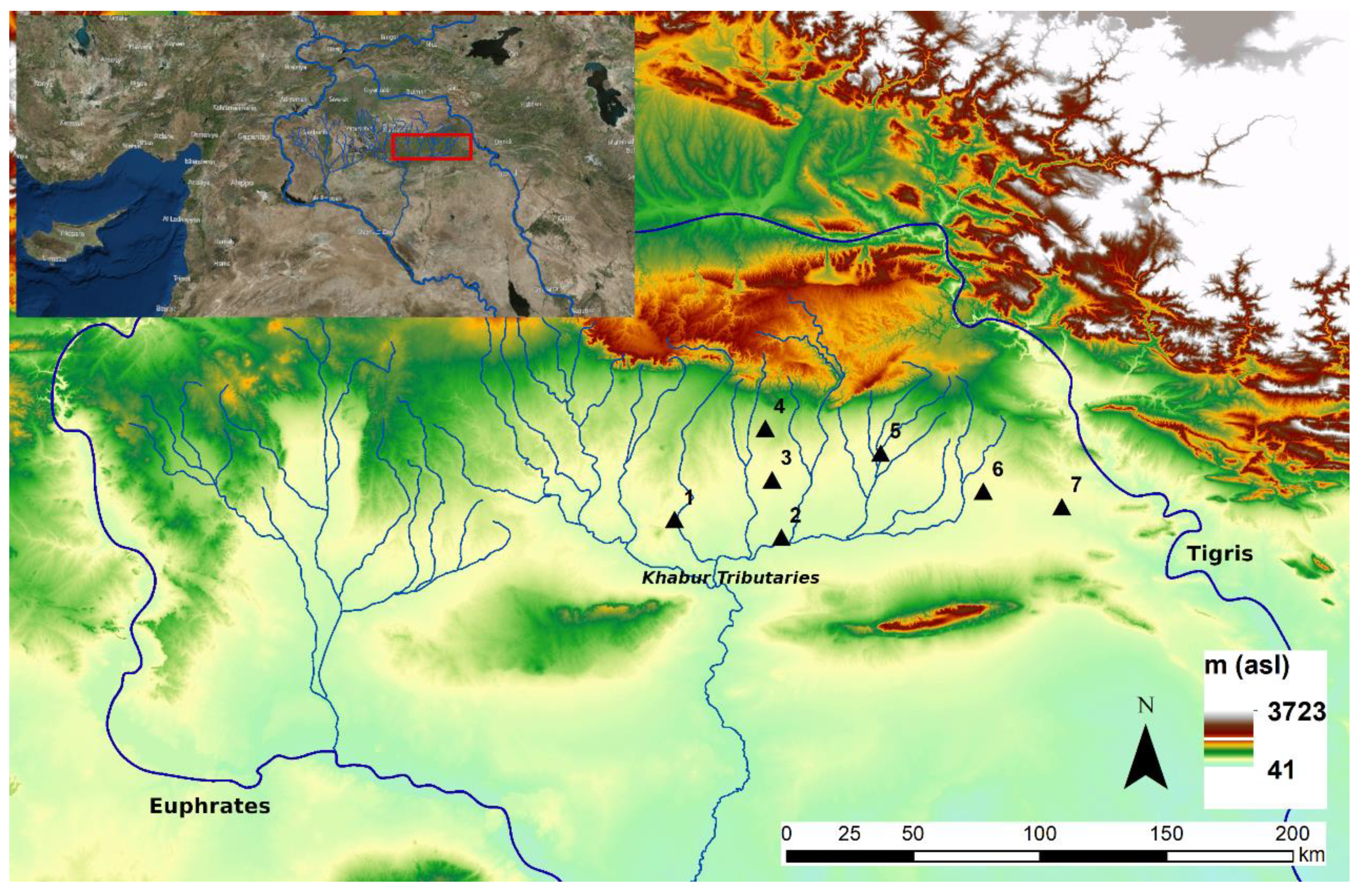
Upper Mesopotamia is the large region between the Tigris River in the east and the Euphrates River in the west (Figure 1). The area is bounded by the Taurus-Zagros Mountains in the north and by desert conditions in the south. The elevation varies between roughly 300 and 600 m asl, but the terrain is relatively flat. The majority of precipitation falls between October–November and April–May. This temporal pattern has a direct impact on modern-day rain-fed agricultural production in the area and how vegetation and soils are manifested in spectral data.
This study focuses on the eastern portion of Upper Mesopotamia. Khabur is the main hydrological feature in this area of interest. It is the largest tributary of the Euphrates River and is mainly formed out of several wadis (easternmost thin blue lines in Figure 1). Ras al Ain, which is one of the largest karst springs in the world, provides most of the discharge for the Khabur.
Upper Mesopotamia has a rich archaeological record dating from the onset of the Neolithic to Medieval times. This paper focuses on the second half of the Early Bronze Age (ca. 2500–2300 BCE; EJ III), when urbanism and intensification of agricultural production shaped the Upper Mesopotamian landscape significantly. In turn, these two socioeconomic factors contributed to the creation of a unique landscape of movement in the form of a dense transportation network between Early Bronze Age sites as well as between settlements and their pasture lands.
First, urbanism introduced a compact way of organizing space. Closely built structures around existing settlement mounds created a new style of habitation. The concentration of population (and animals) resulted in higher movement fluxes from settlements to outer lands, exposing paths to more trampling and compression. Second, Upper Mesopotamian urbanism was mainly possible in regions where dry farming was practiced [33]. Relatively reliable and high levels of precipitation were needed to support dependable agricultural production and, thus, the urban settlement system as a whole. In fact, production was intensified in such a way that rural tributary communities supported extensive populations of large central settlements [34] (pp. 312–314).
Features of Spectral Interest
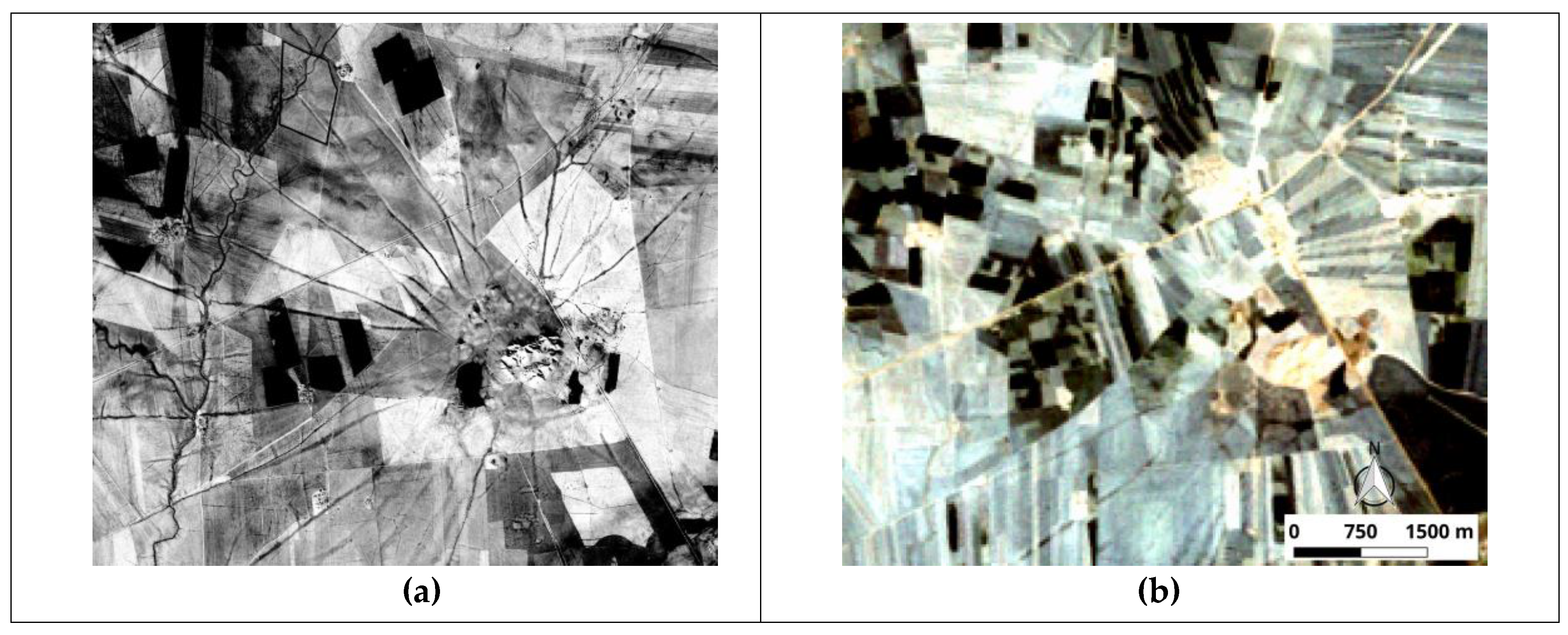
Hollow ways are the markers of intensified agricultural production during the Early Bronze Age (for a detailed analysis of structure and dating, see [35]). These linear features, with widths ranging from 30 to 100 m, radiated from settlements and terminated after an average distance of 2.5 to 3.0 km. In some other cases, they extended further into the landscape and connected settlements to one another. Wilkinson [27] shows that hollow ways were used for the controlled transportation of flocks from settlements to open pastureland. As a result, of continuous foot traffic from animals and humans, linear depressions were formed around settlements. This evidence for repetitive ancient movement still survives today and is visible on satellite imagery (Figure 2a) [36]. A complete digital inventory of hollow ways can be viewed at the Harvard WorldMap project [37] and vectorized hollow-way features can be downloaded for local viewing and analysis in a Geographic Information Systems (GIS) software [38].
This study is based on the axiom that hollow ways have detectable differential moisture-retention capabilities and soil-compaction levels due to their use histories. Roads carrying more traffic must have had more soil compaction (and thus lower moisture-retention capacities) and vice versa. Variations in soil moisture have an immediate impact on reflectance values, as well as soil-productivity levels: vegetation growing above and around hollow ways appears differently in spectral data because of variable access to soil moisture as well as differential root growth due to the compaction of ancient road surfaces (Figure 2b).
Therefore, hollow ways provide a unique opportunity not only for feature mapping, but also for evaluating levels of spectral contrast. This is because their formation and structure are well understood, thanks to previous archaeological research [39]. Second, when preserved, even sensors with coarse spatial resolutions can decipher these features. Third, the linear nature of hollow ways means that they have limited topological-spectral complexity. Fourth, they are situated in a relatively flat and homogeneous terrain, minimizing topographic effects on spectral readings. Finally, there is an immediate relationship between hollow way soils and differential vegetation growth. This paper is an attempt to show how variable precipitation conditions result in a dynamic response of hollow ways on spectral data.
As alternative functional descriptions, some researchers have suggested that a hollow way results from a hydro-compaction process in which where the rupturing of fine soil material initiated the formation of shallow gullies [40]. It has been also argued that these depressions were components of man-made drainage systems [41]. Therefore, it is true that the slope of the ground can be an important determinant for the hollow ways’ spectral reflectance characteristics, especially since the remnants of hollow ways may continue to facilitate surface run-off. Nevertheless, previous research also suggests that hollow ways did not necessarily follow the hydraulic grade [39,42], and so their function in carrying run-off water may be considered unlikely. A systematic evaluation of a high-resolution Digital Elevation Model may further resolve this issue.
2.2. Methodology
2.2.1. Visibility Conditions
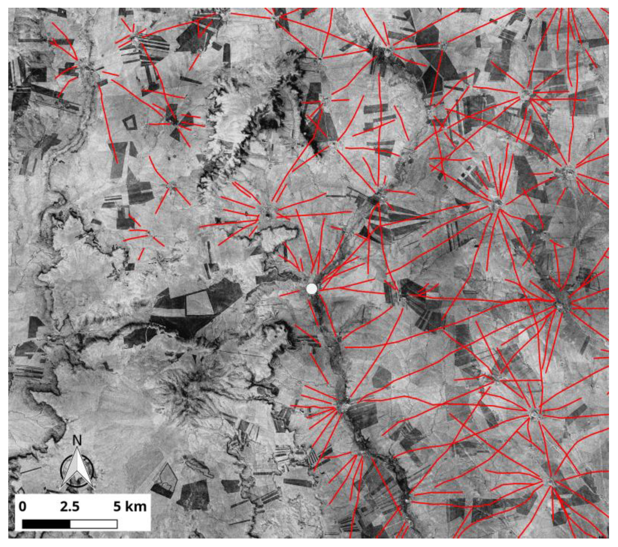
The first step in the methodology is to explore the association between the acquisition date of the satellite data and the spectral visibility of features without considering any prior background information. To illustrate this relationship, Tell Beydar and its wider hinterland (#1 in Figure 1), which are located in the heart of Upper Mesopotamia, are presented as a sub-case study. Hollow ways are not evident in the basaltic environment to the west of the site. This suggests that the underlying geology led to differential conditions of preservation, or perhaps that it played a role in influencing people’s decisions about movement. The existence of a detailed map of hollow ways from Tell Beydar [34] (p. 321) increases the reliability of the visibility analysis (Figure 3).
Hollow ways are documented with the help of the underlying CORONA imagery. Photogrammetrically corrected images were acquired from the CORONA Atlas & Referencing System (http://corona.cast.uark.edu/) and they are orthorectified using SRTM 90m Digital Elevation Model. Next, two commonly used spectral indices in archaeology, the Normalized Difference Vegetation Index (NDVI) and Normalized Difference Water Index (NDWI) were calculated monthly for the years between 2014 and 2017, and annually for the same timeframe. Landsat 8 equipped with the OLI-TIRS sensor (30 m spatial resolution) provided the necessary spectral bands for the operation. Atmospherically corrected reflectance data were acquired from the United States Geological Survey (USGS) EarthExplorer portal. After the visual check for cloud coverage and image quality, spectral indices were calculated using near-infrared (NIR), red, and green bands (see Table A1 in the Appendix A for their formulas).
Spectral indices are calculated for each acquisition date. Monthly values are estimated by a single value if there is only one acquisition in the month, or by an average where there are two or more acquisitions in the month. Finally, monthly indices were averaged for across four years (2014, 2015, 2016, and 2017). The result was two spectral time series (one for NDVI and one for NDWI) from January to December.
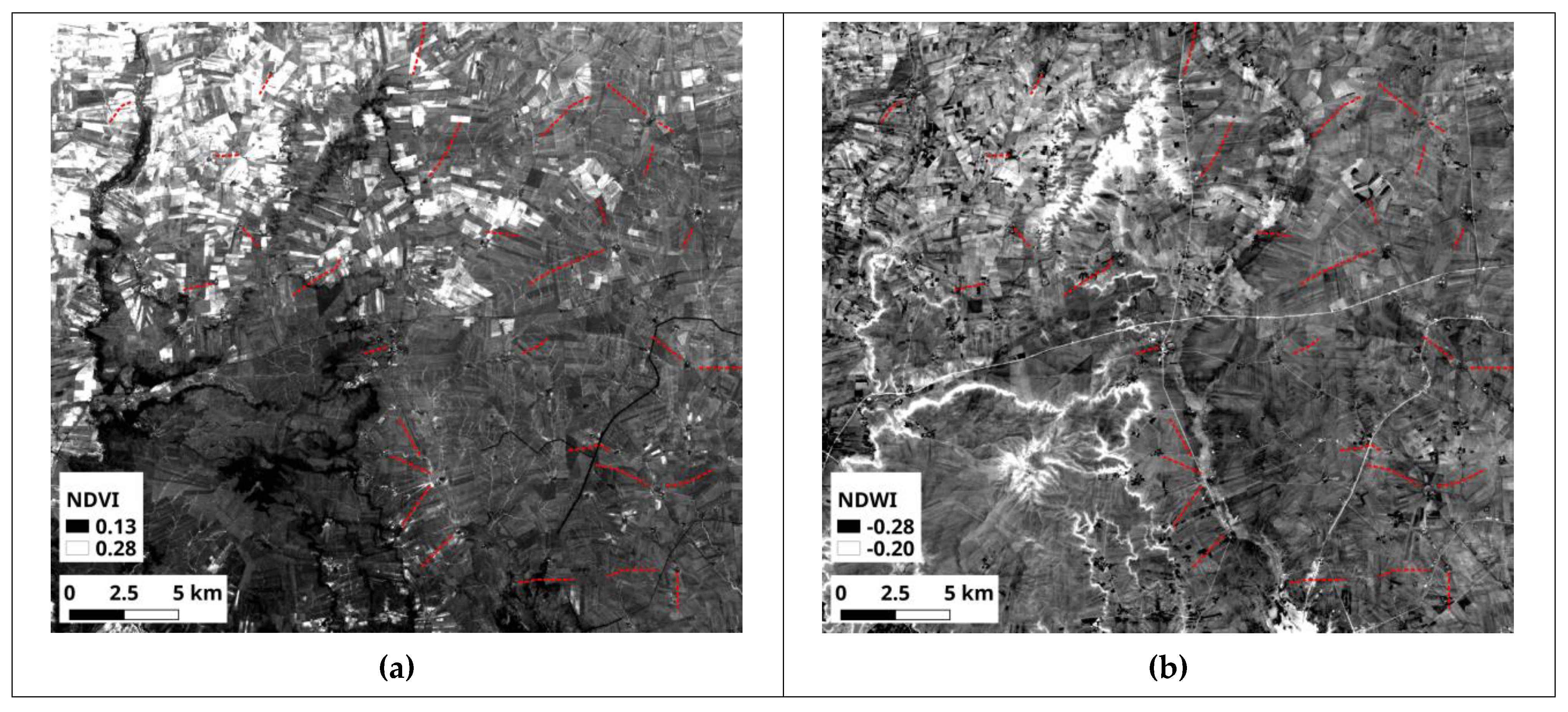
Next, a representative sample of 30 hollow ways in the Tell Beydar hinterland was randomly selected from the main dataset (Figure 4). NDVI and NDWI datasets were manually checked for these hollow ways as there was a reference set showing where hollow way existed. Next, the amount of the hollow way that could be seen is digitized for each monthly set of NDVI and NDWI. Finally, vector lengths were calculated for time-series comparison (Figure 5).
Based on the inferences from the time-series comparison, the focus of analyses shifted to May and November in order to investigate how precipitation impacts the spectral contrast of the features while maximizing the likelihood of discriminating the hollow ways in length (Section 2.2.3). Furthermore, other sample areas were integrated into the study in order to evaluate different geographic conditions (Figure 6). Finally, a large set of spectral indices were calculated to represent most of the electromagnetic spectrum, and how these indices perform under different precipitation levels was investigated.
2.2.2. Precipitation Dataset
The precipitation dataset was obtained for the years between 1981 and 2010 from the Global Precipitation Climatology Center (GPCC) at the Deutscher Wetterdienst (Schneider et al. 2011). For the best spatial representation, grids with 0.5 degrees separation were converted to monthly precipitation surfaces using natural neighborhood interpolation. The sample areas were then clipped from these raster layers. To better describe the regime, cumulative rainfall statistics from areas were calculated from December to May (cumulatively called May) and from June to November (cumulatively called November) and averaged for the region (Figure 7). This average accurately describes the precipitation regime of the study region (the eastern portion of Upper Mesopotamia), as sample areas have an even distribution. Finally, four statistics (minimum, low, high, and maximum) are selected to represent the time-series.
2.2.3. Building Spectral Indices
Following the calculation of precipitation statistics in sample areas, 25 indices were generated (Table A1) [43,44]. This inclusive stance allowed for the creation of many different algebraic combinations of bands representing the electromagnetic spectrum fully in an undiscriminating manner. Following an inductive approach, the initial aim is to look for patterns where seemingly discrete indices converge and explain the differences in spectral contrast between the hollow ways and their immediate surroundings. Also, a high degree of similarity between different bands can cause redundancies in spectral data analysis. However, as the first comprehensive study of the spectral index characterization of hollow ways distributed in a vast study area, the methodology investigates potential minute differences between the indices. In fact, data reduction is particularly avoided, since the proposed comparison is not within different index values, but rather between index values and precipitation levels.
The spectral data were taken from NASA’s Landsat mission due to its consistency, overall reliability, and length of records. The mission provides spectral data for the available range of precipitation time-series (1981–2010). Using a single system also minimizes compatibility issues between band designations in different satellite missions. The Landsat 4–5 Thematic Mapper (TM) duo was in operation from 1982 to 2013. Landsat 7 with Enhanced Thematic Mapper Plus (ETM+) was launched in 1999 and continues its mission. However, due to the failure of the Scan Line Collector (SLC) in 2003, scenes collected after this date have data gaps. For this reason, Landsat 7 was not used for analysis of dates following this year. All spectral bands (blue, green, red, near infrared, shortwave infrared 1, shortwave infrared 2) have a resolution of 30 m and were obtained from the USGS as atmospherically corrected surface reflectance products.
Like any other passive satellite system, the Landsat mission suffers from cloud coverage. Also, some scenes are not usable due to instrumental error. In other cases, hazy conditions or atmospheric dust reduce the image quality, and the error is propagated from the original spectral bands to calculated index products. Therefore, it is not always possible to use a specific date in satellite remote sensing analysis which is best fitting the needs of the research question, and this type of study is prone to these problems; that is, the timing of a precipitation statistic date did not always match with the date of a high-quality Landsat scene.
In the case of low spectral data quality, the next available Landsat scene was picked. For instance, cumulated November produced the most rains in 2006 (Figure 7), but the matching Landsat scene was of low quality. The next best month describing maximum precipitation was in 1987, but again, there was no operational Landsat scene available. Ultimately, the November collection from 1988 was used instead. Table 1 shows the available high-quality eight Landsat captures with minimum cloud coverage. These images were used to calculate the 25 spectral indices mentioned below.
Landsat bands were fed into a custom-built Python 3.5 code in batch-processing mode. Six spectral bands (blue, green, red, near-infrared, short-wave infrared 1, and shortwave infrared 2) produced 25 broad-band spectral indices for each sample area and for each of the eight dates with minimum, low, high, and maximum precipitation in May and November. 25 indices for seven sample areas and for eight precipitation dates resulted in 1400 different indices. As an intermediary quality-control step, indices were visually investigated following their production and low-quality datasets were removed from the workflow.
While May scenes produced high-quality spectral indices ready for statistical analysis, November scenes failed to produce operational data other than GDVI, MNLI, NDMI and WET. It is possible that the previous generation Landsat sensors (and their calibrations) were not able compensate for the atmospheric effects as much as the Landsat 8. This is exemplified in Figure 8, the OLI sensor can produce very high-quality NDVI datasets (as used in Section 2.2.1), whereas previous-generation Landsat sensors produce data that does not allow for a detailed spectral analysis of archaeological features.
2.2.4. Generation of Vector Data
A total of 56 Landsat sub-scenes were analyzed (eight points in time for each of the seven sample areas; see Table 1) and the visible hollow ways were manually digitized in each scene. For the digitization, only the reflectance bands (blue, green, red, near infrared, shortwave infrared 1, and shortwave infrared 2) were used as references. If the hollow way was cutting through distinctly homogeneous spectral groups (such as two agricultural fields one vegetated and one barren), only the largest portion falling within a single spectral group was digitized in order to minimize within-group variance. Next, the vectorized features were divided into 10-m intervals and corresponding nodes were stored in a single point vector file. Finally, values from each of the 25 indices were recorded at sample locations (i.e., the nodes) and data-arrays were formed for statistical analysis.
To determine the level of spectral contrast between a feature and its immediate background, 100-m-wide rectangular buffer zones were created around each hollow way in order to sample from their local backgrounds. A random sample was selected within each buffer zone, dynamically matching the sample size of the corresponding hollow way nodes. Focusing only on local backgrounds minimizes pedological complexity and decreases the potential impact of differential land-use practices in areas away from hollow ways (Figure 9).
Spectral readings of background buffers and hollow ways were merged for each sample area. Next, data falling outside of 3 standard deviations were removed to reduce potential sensor errors and to maximize between-group variations between hollow ways and their corresponding backgrounds. To statistically evaluate the level of spectral contrast for each index, Welch’s t-test (assuming unequal variances) was used. The null hypothesis was that the spectral values of hollow ways and the spectral values of their immediate backgrounds have equal mean values (for α = 0.01), and thus, hollow ways are not separable spectrally.
The results of this test indicate which spectral indices provide statistically significant feature contrast at sample areas (Table A2 in the Appendix B). Non-significant results are still valuable for mapping purposes, as the hollow ways are sometimes visible to the naked eye (as spatial manifestations of subtle contrast differences). However, further quantitative analysis cannot be performed using these indices. Therefore, the following steps were followed only using spectral indices which provided significant levels of contrast.
Since there was only a small number of high-quality indices dating to November (GDVI, MNLI, NDMI, and WET), it was not possible to conduct a comparative analysis between the two months. Furthermore, the discrepancy between their sample sizes necessitated the use of different statistical methods. For November, tabulating the spectrally significant indices from the seven sample areas resulted in a 4x4 contingency table with count data (Table 2). To investigate whether a proportion of one of the nominal variables (i.e., the spectral index) differs from the values of the other variable, the Fisher’s exact test of independence was deployed in R 3.5.
The spectral indices from May were sufficient in number. A Correspondence Analysis (CA) was also performed using tabulated indices. First, the significant indices were totaled for each of the seven sample areas and a summary table generated (Table 3). Out of the 25 indices, the Moisture Stress Index (MSI) and Non-Linear Index (NLI) did not produce any significant spectral contrast between the hollow ways and their immediate environments. The CA was applied to the count of significant indices in order to understand the relationship between the spectral responses and precipitation regime.
3. Results
3.1. Visibility Conditions in Time Series
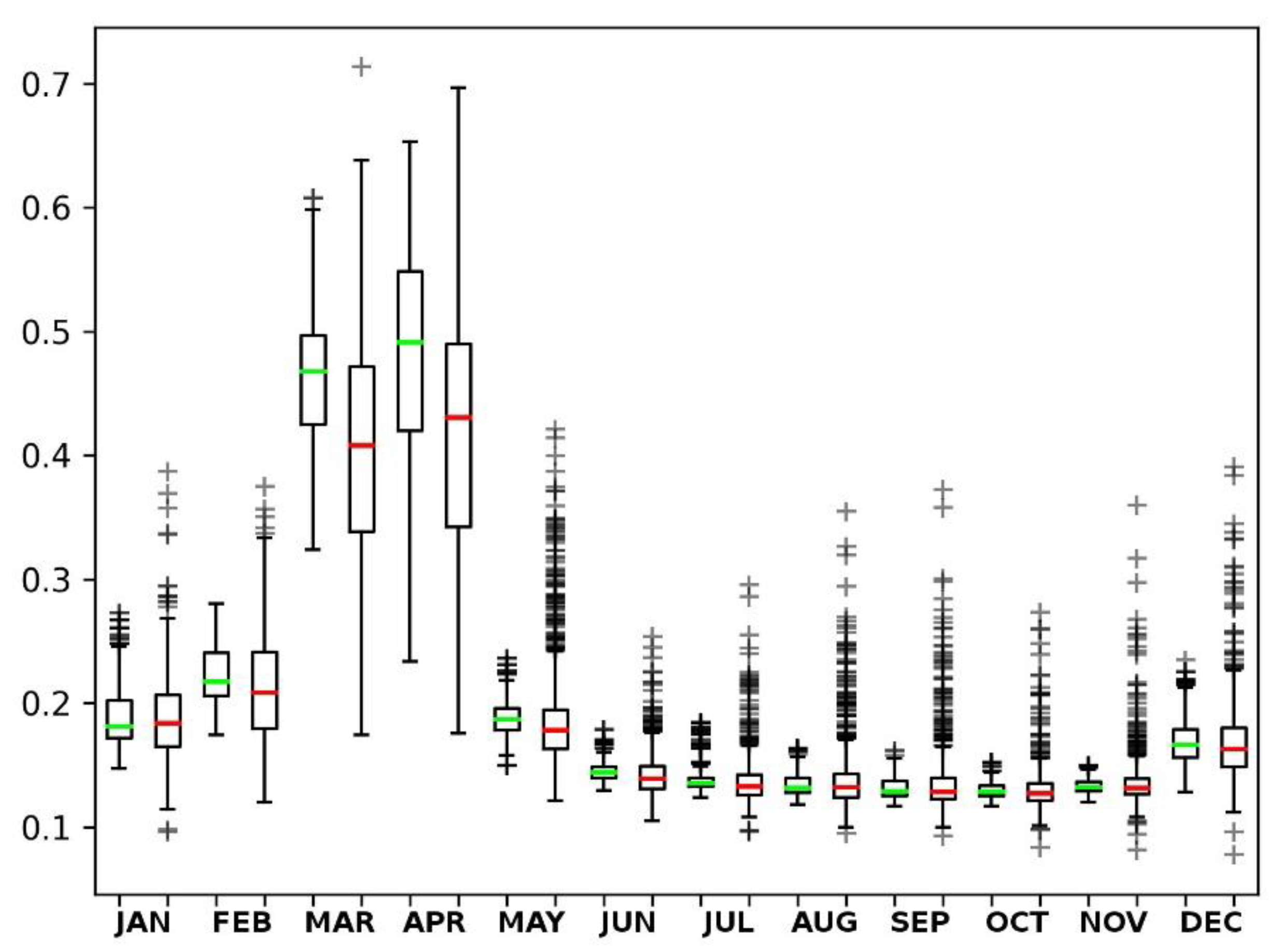
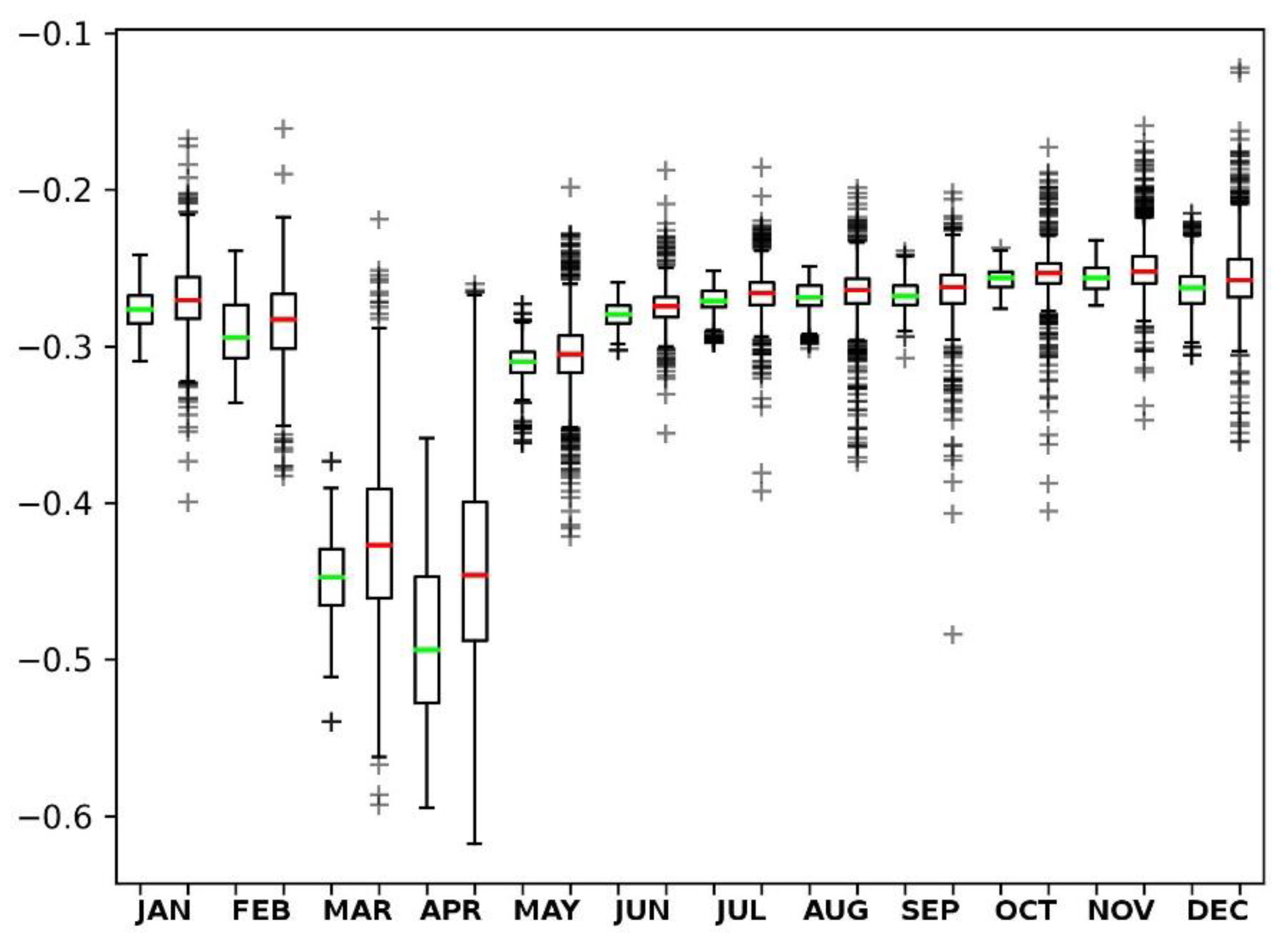
The time-series investigation of NDVI values in comparison to the average spectral background suggests that vegetation heading and flowering took place during March and April, and crops rapidly transitioned into ripening stage in May (Figure 10). Therefore, what makes hollow ways more visible (i.e., spatially separable) is, in fact, not directly related to the vegetation health as measured (and commonly used) by NDVI, since May is the month when hollow ways are most easily detected by the naked eye. A similar interpretation is possible for the monthly NDWI values of hollow ways and their respective background values from each scene (Figure 11). Hollow ways are most visible to the naked eye in November, but again, the NDWI average spectral contrast between hollow ways and their backgrounds is highest during March and April.
3.2. Evaluation of Spectral Indices
The tabulated data highlight two indices that provide most of the spectral contrast for the sample areas in November: MNLI and NDMI (Table 3). Fisher’s exact test for count data yields a simulated p-value of 0.9191 based on 1000 replicates. This is a highly insignificant result, so one can almost certainly conclude that there is no relation between the precipitation levels and the four spectral indices under consideration.
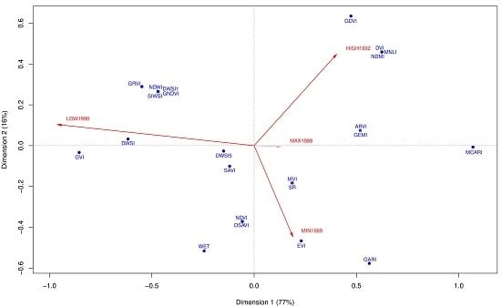
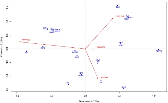
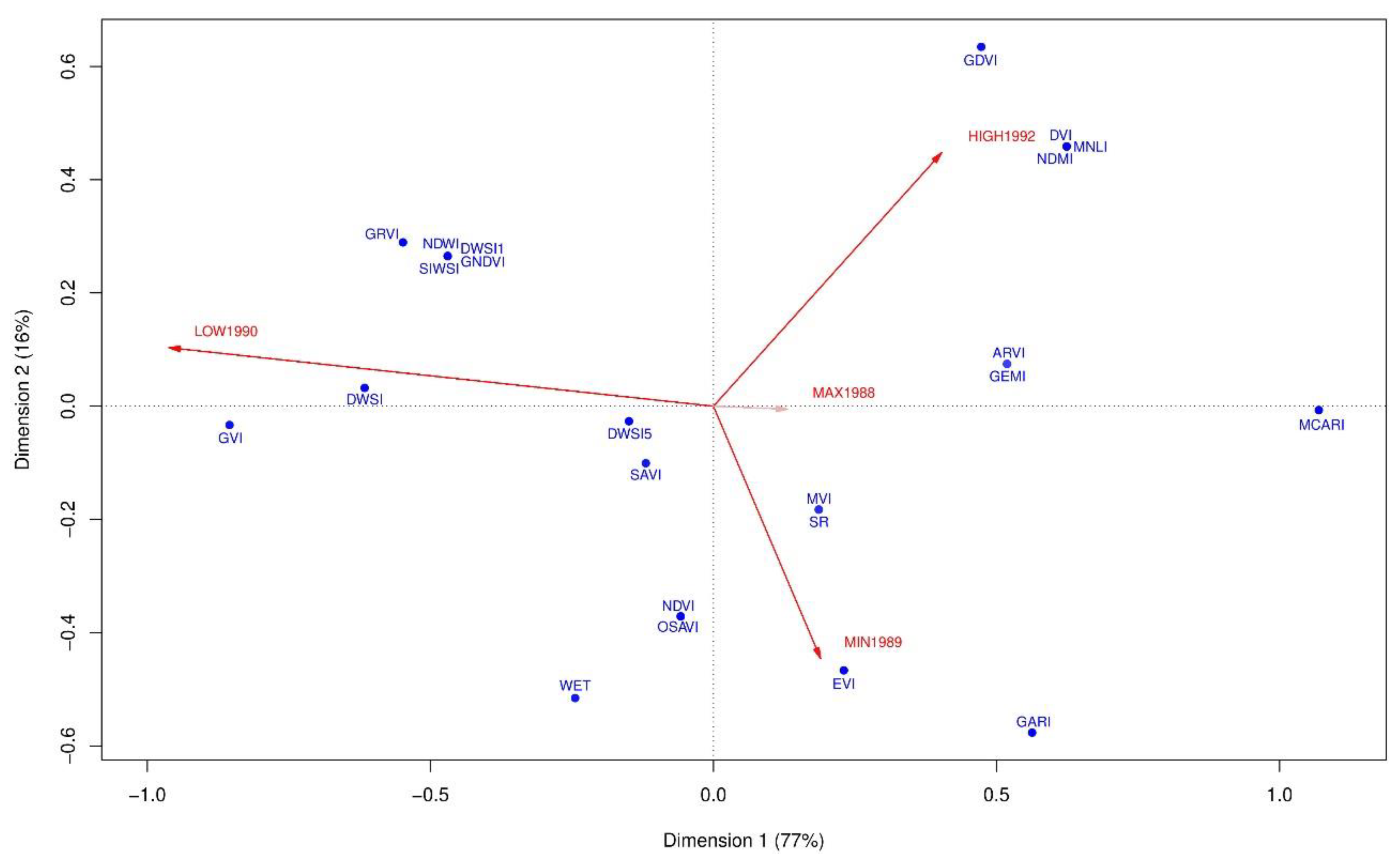
The spring season provides more room for exploration. The Correspondence Analysis (CA) explain 93 % of the variation in the data (Figure 12). Thus, the interpretation rests on a strong base. In May 1988 (the maximum precipitation) the spectral indices perform equally. Therefore, maximum precipitation is a weak determinant for choosing an ideal index; the CA positions May 1988 very close to the origin, supporting this claim. The rest of the dates corresponding to minimum, low, and high precipitation values span the correspondence space equally and are farther away from the origin. It can be concluded that these three dates explain most of the variation in the contrast performance of the spectral indices. DWSI5, SAVI, MVI, and SR are clustered around the origin, suggesting that these indices perform equally under variable precipitation conditions; they discriminate the least between spectral contrast and rainfall. In fact, DWSI5 performs the best, but it also evenly contributes to correspondence (min rainfall: 5, low: 4, high: 4, max: 5).
The precipitation dates relative to the index values and their groupings reveal further relations. For instance, the Enhanced Vegetation Index (EVI) is the most discriminating when rainfall is at minimum levels. The CA also suggests that there is considerable clustering for different precipitation conditions. Under high precipitation (in 1992) GDVI, DVI, MNLI, and NDMI perform similarly, and one may use GVI but avoid MCARI under low precipitation.
The analysis further reveals five distinct groups of spectral indices: (1) DVI, MNLI, NDMI; (2) ARVI, GEMI; (3) MVI, SR; (4) NDVI, OSAVI; and (5) GRVI, NDVI, DWSI1, GNDVI, SIWSI. Among these, Group 1 can be associated with high precipitation values in 1992, Group 4 with minimum precipitations in 1989 and Group 5 with low precipitation levels in 1990. Correlation matrices (Table A3 in the Appendix B) reveal high degree of correlations for all of the sample areas. For some of the index couples, such as NDWI and GNDVI, this is an expected result, as their algebraic band combinations mimic each other. In other cases, a different spectral combination can still demonstrate a strong (albeit negative) association, such as that between NDWI and DWSI1.
4. Discussion
Contrast—as a concept—becomes even more fruitful as the interest shifts from the spatial domain (what is immediately visible as a hollow way, the “contrast”) to the spectral domain (the average spectral separation of a hollow way from its background, the “level of contrast”). Figure 10 and Figure 11 suggest that higher average spectral separation of hollow ways from the overall scene does not necessarily translate into higher feature visibility. This is also to say that the assumed link between spatial contrast and spectral contrast does not always hold, especially as one moves from the larger scene to local conditions. This breaks the false pre-eminence of the global spectral scene over local conditions, especially when date of satellite data acquisition is determined; the choice may not be determined by overall vegetation health or optimal climatic conditions.
When investigated in time-series form, the relationship between the acquisition date of a scene and the visibility of the hollow ways is most obvious in May and November. However, in November, NDWI clearly outperforms NDVI, probably due to the impact of first rains after a long and very dry period in the summer. It is also important to note that even during summer months, NDVI provides better background for mapping than in spring when the crop vegetation is the greenest. Two deductions can be made based on these observations: first, hollow ways are easier to detect with soil marks than with vegetation marks. This result also implicitly suggests that the differences in soil moisture retention capacities of hollow ways do not fully translate into differences in vegetation health. Second, despite their lower values, the vegetation index can still solve for hollow ways. In these cases, the index does not necessarily represent crop vegetation, but more probably the presence of drought- and salinity-resistant Prosopis type green shrubs [39] that grow along the axis of hollow ways and create distinctive alignments. Therefore, vegetation indices still remain useful for the detection of hollow ways.
Lagging is a concern when spectral data is investigated in a time-series [45,46]. Scarcity or abundance of rainfall may not immediately affect the crop growth. Thus, the vegetation indices may carry a “lag”, which offsets the relationship between precipitation and the spectral response characteristics. Lagging is not only specific to geographical areas, but also to different plant species: different types of vegetation growing in the same area may have different tolerance levels to variations in water availability. Furthermore, even for the same type of crop the lag lengths can differ between the early and late growing seasons. Finally, studies usually report lags only for a couple of indices [47]. Considering the complexity of lagging calculations, the vast size of the study area under investigation, and the high number of spectral indices under consideration, integrating lagging into the analysis is beyond the scope of the project at this stage. Despite its coarser resolution (30 m), Landsat multispectral imagery is not only useful for mapping hollow ways, but also for discriminating between hollow ways with different levels of contrast. In fact, there are newer sensors which provide higher spatial (and spectral) resolution such as Sentinel 2, but Landsat is unique for its historicity. Providing Earth Observation as early as 1972, there is no other system which has been so instrumental in providing time-series analysis as the one used in this study.
Newer multispectral sensors with higher spatial resolutions may lack the temporal depth, but preserved hollow ways appear in greater detail. Publicly available Sentinel 2 data, for instance, provide higher spectral representation of Near Infrared portion of the electromagnetic spectrum represented in three near edge (vegetation) bands and two Near Infrared bands compared to Landsat missions. Furthermore, it has superior temporal resolution with five days revisiting period. This level of precision opens up new research paths for a detailed analysis of the relationship between climatic conditions and the spectral representation of archaeological features. The commercial satellite WorldView-3 has even higher spatial resolution (1.24 m multispectral, 3.7 m shortwave; Figure 13). In particular, the availability of eight shortwave-infrared bands brings the possibility of modeling soil moisture content in detail.
Increases in sensor spectral, spatial, and temporal resolutions may lead towards a theory of archaeological satellite remote sensing. In particular, empirical models of hydraulic conductivity and soil moisture storage capacity of cultural soils [48] coupled with spectral data analysis can highlight replicable and testable physical relationships between archaeological features and the ways in which they are reflected on electromagnetic spectrum. Ancient hollow ways are promising features in this respect. Detailed geomorphological evaluation of these linear features within the context of satellite remote sensing, e.g., how much they withstood erosion, or how much they facilitated/blocked surface runoff [49] might also highlight emergence, use, and abandonment, as well as post-depositional phases. After all, what is measured by a spectral sensor is not the actual road surface, but the relic of the road which has been transformed considerably [50].
5. Conclusions
Publicly available multispectral sensor data with increasingly high spatial resolutions call for a wider use of spectral indices in archaeology. Due to these developments, it is also possible to conduct comparative quantitative performance analyses for large areas under varying climatic and geographic conditions. As increasing amounts of spatially accurate survey and excavation data becomes available to researchers in digital forms, it is a feasible task to systematically explore how the light behaves when reflected and/or emitted from archaeological features (or from their proxies) under variable background conditions. Therefore, the use of a specific spectral index in an archaeological investigation can and should be justified [51].
The reduction in prices of archived high-resolution commercial satellite images and the widespread use of online viewing platforms makes remote sensing from space more applicable to vast regions than before. Increases in the extent of study areas also call for the use of generic workflows in order to analyses large datasets. On the one hand, satellite remote sensing provides researchers the opportunity to conduct large-scale research in which a global understanding of an archaeological phenomenon is possible. On the other hand, the analysis heavily relies on local conditions, and thus, migrating workflows or carrying the same research parameters to other areas is never a trivial task. For these reasons, building robust methodologies for spectral data with anthropogenic origins remains a significant challenge [52]. This paper is yet another quantitative reminder of how even seemingly homogeneous areas with similar features can produce great diversities in spectral responses.
This study affirms that the contrast is an important determinant in archaeological remote sensing studies; however, it further claims that it is a necessary—but not sufficient—condition if one wants to go beyond mapping projects only using the spatial manifestations of spectral contrast. Understanding the levels of separation makes it possible to categorize features and, thus, adds the necessary dynamism to the archaeological landscape, since every feature carries the potential to be unique according to one category or another.
Author Contributions
Conceptualization, T.K., R.L., J.W. and N.M.; methodology, T.K.; formal analysis, T.K.; writing—original draft preparation, T.K.; writing—review and editing, T.K., R.L., J.W. and N.M.; project administration, N.M., J.W.; funding acquisition, T.K.
Funding
This research was funded by the Marie Skłodowska-Curie Action, Individual Fellowship (IF). The project title is Modern Geospatial Practices for Ancient Movement Praxis (GeoMOP) with the grant number 747793.
Conflicts of Interest
The authors declare no conflict of interest.
Appendix A

Table A1.
The 25 broad-band indices calculated for eight scenes and for seven sample areas, their common abbreviations, and formulas.
Table A1.
The 25 broad-band indices calculated for eight scenes and for seven sample areas, their common abbreviations, and formulas.
| Atmospherically Resistant Vegetation Index | ARVI | [NIR − (RED − gam × (BLUE − RED))]/[NIR + (RED − gam × (BLUE − RED))]; gam = 1 |
| Difference Vegetation Index | DVI | NIR − RED |
| Disease Water Stress Index | DWSI | [NIR + GREEN]/[SWIR2 + RED] |
| Disease Water Stress Index − 1 | DWSI1 | NIR/SWIR2 |
| Disease Water Stress Index − 5 | DWSI5 | [NIR − GREEN]/[SWIR2 + RED] |
| Enhanced Vegetation Index | EVI | [NIR − RED]/[NIR + 6 × RED − 7.5 × BLUE + 1] |
| Green Atmospherically Resistant Index | GARI | [NIR − (GREEN − gam × (BLUE − RED))]/[NIR + (GREEN − gam × (BLUE − RED))]; gam = 1.7 |
| Green Difference Vegetation Index | GDVI | NIR − GREEN |
| Global Environmental Monitoring Index | GEMI | c1 − [RED − 0.125]/[1 − RED]; e1 = 2 × (NIR × NIR − RED × RED) + 1.5 × NIR + 0.5 × RED and e2 = NIR + RED + 0.5; c1 = e1/e2 × (1 − 0.25 × e1/e2) |
| Green Normalized Difference Vegetation Index | GNDVI | [NIR − GREEN]/[NIR + GREEN] |
| Green Ratio Vegetation Index | GRVI | NIR/GREEN |
| Green Vegetation Index | GVI | (–0.2848)BLUE + (–0.2435)GREEN + (–0.5436)RED + (0.7243)NIR + (0.084)SWIR1 + (–0.18)SWIR2 |
| Modified Chlorophyll Absorption in Reflectance | MCARI | 1.2 × (2.5 × (NIR − RED) − 1.3 × (NIR − GREEN)) |
| Modified Non-Linear Index | MNLI | [(NIR × NIR − RED) × (1+L)]/[NIR × NIR + RED + L]; L = 0.5 |
| Moisture Stress Index | MSI | SWIR2/NIR |
| Mid-Infrared Vegetation Index | MVI | NIR/SWIR1 |
| Normalized Difference Moisture Index | NDMI | [NIR − SWIR1]/[NIR + SWIR1] |
| Normalized Difference Vegetation Index | NDVI | [NIR − RED]/[NIR + RED] |
| Normalized Difference Water Index | NDWI | [GREEN − NIR]/[GREEN + NIR] |
| Non-Linear Index | NLI | [NIR × NIR - RED]/[NIR × NIR + RED] |
| Optimized Soil Adjusted Vegetation Index | OSAVI | [1.5 × (NIR − RED)]/[NIR + RED + 0.16] |
| Soil Adjusted Vegetation Index | SAVI | [1.5 × (NIR − RED)]/[NIR + RED + 0.5] |
| Shortwave Infrared Water Stress Index | SIWSI | [NIR − SWIR2]/[NIR + SWIR2] |
| Simple Ratio | SR | NIR/RED |
| Wetness | WET | (0.1509)BLUE + (0.1973)GREEN + (0.3279)RED + (0.3406)NIR − (0.7112)SWIR1 − (0.4572)SWIR2 |
Appendix B
Table A2.
p-values of Welch’s t-test for sub-regions.
| #1 Tell Beydar | |||||||
| 1989MAY | 1990MAY | 1992MAY | 1988MAY | ||||
| 1.07 × 10⁻¹⁹ | NDMI | 2.79 × 10⁻¹⁹ | GVI | 2.54 × 10⁻²² | DWSI | 9.32 × 10⁻¹⁷ | DVI |
| 1.57 × 10⁻¹⁹ | MNLI | 1.53 × 10⁻¹⁷ | DWSI5 | 1.51 × 10⁻¹⁹ | MVI | 4.56 × 10⁻¹⁶ | GEMI |
| 7.06 × 10⁻¹⁹ | DWSI | 1.76 × 10⁻¹⁷ | WET | 2.63 × 10⁻¹⁸ | GVI | 3.85 × 10⁻¹³ | MCARI1 |
| 9.11 × 10⁻¹⁶ | MVI | 3.48 × 10⁻¹⁶ | MSI | 1.31 × 10⁻¹⁷ | DWSI5 | 2.13 × 10⁻¹² | SR |
| 1.12 × 10⁻¹⁵ | DVI | 2.29 × 10⁻¹⁴ | DWSI | 2.75 × 10⁻¹⁶ | SIWSI | 6.41 × 10⁻¹² | GVI |
| 3.71 × 10⁻¹⁵ | GEMI | 1.32 × 10⁻¹¹ | SIWSI | 3.94 × 10⁻¹⁶ | DWSI1 | 1.01 × 10⁻¹¹ | SAVI |
| 9.63 × 10⁻¹⁵ | EVI | 3.19 × 10⁻¹¹ | DWSI1 | 2.07 × 10⁻¹⁴ | GNDVI | 1.01 × 10⁻¹¹ | OSAVI |
| 3.34 × 10⁻¹³ | GARI | 3.16 × 10⁻⁸ | GRVI | 2.07 × 10⁻¹⁴ | NDWI | 1.01 × 10⁻¹¹ | NDVI |
| 5.12 × 10⁻¹² | SAVI | 5.14 × 10⁻⁸ | GNDVI | 2.75 × 10⁻¹⁴ | GRVI | 3.22 × 10⁻¹⁰ | GRVI |
| 5.12 × 10⁻¹² | OSAVI | 5.14 × 10⁻⁸ | NDWI | 2.34 × 10⁻¹³ | SR | 5.62 × 10⁻¹⁰ | ARVI |
| 5.12 × 10⁻¹² | NDVI | 1.58 × 10⁻² | GDVI | 3.05 × 10⁻¹³ | DVI | 8.73 × 10⁻¹⁰ | DWSI5 |
| 1.10 × 10⁻¹¹ | SR | 3.56 × 10⁻¹³ | GEMI | 1.29 × 10⁻⁹ | NDWI | ||
| 1.36 × 10⁻¹⁰ | DWSI1 | 3.97 × 10⁻¹³ | NDVI | 1.29 × 10⁻⁹ | GNDVI | ||
| 1.88 × 10⁻¹⁰ | SIWSI | 3.97 × 10⁻¹³ | OSAVI | 2.55 × 10⁻⁹ | GARI | ||
| 1.92 × 10⁻¹⁰ | GDVI | 3.97 × 10⁻¹³ | SAVI | 6.60 × 10⁻⁹ | EVI | ||
| 3.36 × 10⁻¹⁰ | GVI | 1.12 × 10⁻¹² | GARI | 6.88 × 10⁻⁸ | DWSI | ||
| 3.59 × 10⁻⁷ | DWSI5 | 1.50 × 10⁻¹² | WET | 9.73 × 10⁻⁷ | MVI | ||
| 3.77 × 10⁻⁷ | WET | 3.81 × 10⁻¹² | ARVI | 1.66 × 10⁻⁶ | SIWSI | ||
| 2.51 × 10⁻⁵ | NDWI | 1.07 × 10⁻¹¹ | MNLI | 2.56 × 10⁻⁶ | DWSI1 | ||
| 2.51 × 10⁻⁵ | GNDVI | 1.14 × 10⁻¹¹ | EVI | 3.10 × 10⁻⁴ | WET | ||
| 2.97 × 10⁻⁵ | GRVI | 1.14 × 10⁻¹¹ | NDMI | 1.41 × 10⁻² | NDMI | ||
| 3.35 × 10⁻¹¹ | MCARI1 | 1.41 × 10⁻² | MNLI | ||||
| 3.83 × 10⁻⁹ | GDVI | ||||||
| #2 Tell Brak | |||||||
| 1989MAY | 1990MAY | 1992MAY | 1988MAY | ||||
| 1.87 × 10⁻⁷ | WET | 1.79 × 10⁻¹³ | GARI | 8.19 × 10⁻³ | MNLI | 4.17 × 10⁻³² | SIWSI |
| 8.89 × 10⁻⁴ | ARVI | 1.81 × 10⁻¹³ | NDVI | 8.57 × 10⁻³ | DVI | 5.83 × 10⁻³² | DWSI1 |
| 1.09 × 10⁻³ | GARI | 1.81 × 10⁻¹³ | SAVI | 8.66 × 10⁻³ | NDMI | 3.01 × 10⁻²⁹ | DWSI |
| 1.88 × 10⁻³ | MCARI1 | 1.81 × 10⁻¹³ | OSAVI | 1.63 × 10⁻² | DWSI5 | 3.65 × 10⁻²⁹ | WET |
| 5.33 × 10⁻³ | EVI | 2.26 × 10⁻¹³ | ARVI | 2.21 × 10⁻² | MCARI1 | 1.17 × 10⁻²⁴ | ARVI |
| 6.20 × 10⁻³ | DWSI5 | 3.96 × 10⁻¹³ | EVI | 2.33 × 10⁻²⁴ | EVI | ||
| 1.62 × 10⁻² | NDVI | 1.01 × 10⁻¹¹ | SR | 7.84 × 10⁻²⁴ | GARI | ||
| 1.62 × 10⁻² | OSAVI | 4.57 × 10⁻¹¹ | GVI | 2.93 × 10⁻²³ | DWSI5 | ||
| 1.62 × 10⁻² | SAVI | 1.77 × 10⁻⁹ | DWSI5 | 1.29 × 10⁻²² | GVI | ||
| 3.87 × 10⁻⁹ | WET | 1.90 × 10⁻²² | MCARI1 | ||||
| 2.86 × 10⁻⁸ | GRVI | 1.32 × 10⁻²⁰ | NDVI | ||||
| 2.95 × 10⁻⁸ | GEMI | 1.32 × 10⁻²⁰ | OSAVI | ||||
| 6.72 × 10⁻⁸ | DVI | 1.32 × 10⁻²⁰ | SAVI | ||||
| 8.94 × 10⁻⁸ | DWSI | 2.01 × 10⁻²⁰ | SR | ||||
| 1.02 × 10⁻⁷ | GNDVI | 4.76 × 10⁻²⁰ | MVI | ||||
| 1.02 × 10⁻⁷ | NDWI | 5.75 × 10⁻¹⁹ | DVI | ||||
| 5.44 × 10⁻⁷ | SIWSI | 3.48 × 10⁻¹⁸ | GRVI | ||||
| 8.87 × 10⁻⁷ | DWSI1 | 7.92 × 10⁻¹⁸ | GNDVI | ||||
| 5.38 × 10⁻⁶ | MVI | 7.92 × 10⁻¹⁸ | NDWI | ||||
| 3.53 × 10⁻¹⁷ | GEMI | ||||||
| 1.74 × 10⁻¹⁰ | NDMI | ||||||
| 1.97 × 10⁻¹⁰ | MNLI | ||||||
| 6.58 × 10⁻⁶ | GDVI | ||||||
| #3 Tell Arbid | |||||||
| 1989MAY | 1990MAY | 1992MAY | 1988MAY | ||||
| 3.68 × 10⁻⁷ | NDMI | 2.97 × 10⁻⁴ | SR | 7.02 × 10⁻¹⁵ | WET | 1.54 × 10⁻² | GEMI |
| 4.15 × 10⁻⁷ | MNLI | 8.73 × 10⁻⁴ | NDVI | 7.85 × 10⁻¹³ | SIWSI | ||
| 3.02 × 10⁻⁶ | MCARI1 | 8.73 × 10⁻⁴ | OSAVI | 8.55 × 10⁻¹² | DWSI1 | ||
| 6.79 × 10⁻⁶ | DVI | 8.73 × 10⁻⁴ | SAVI | 1.23 × 10⁻¹¹ | DWSI | ||
| 3.07 × 10⁻⁵ | GEMI | 1.69 × 10⁻³ | DWSI | 8.39 × 10⁻¹⁰ | MVI | ||
| 6.07 × 10⁻⁵ | SR | 1.77 × 10⁻³ | GVI | 1.27 × 10⁻⁹ | DWSI5 | ||
| 8.92 × 10⁻⁵ | EVI | 2.09 × 10⁻³ | GNDVI | 9.00 × 10⁻⁹ | ARVI | ||
| 2.59 × 10⁻⁴ | GVI | 2.09 × 10⁻³ | NDWI | 1.22 × 10⁻⁸ | EVI | ||
| 2.90 × 10⁻⁴ | MVI | 2.37 × 10⁻³ | GRVI | 2.53 × 10⁻⁸ | MCARI1 | ||
| 2.94 × 10⁻⁴ | GARI | 6.72 × 10⁻³ | EVI | 1.64 × 10⁻⁷ | SR | ||
| 3.76 × 10⁻⁴ | OSAVI | 7.05 × 10⁻³ | DWSI1 | 1.65 × 10⁻⁷ | NDVI | ||
| 3.76 × 10⁻⁴ | SAVI | 9.32 × 10⁻³ | WET | 1.65 × 10⁻⁷ | OSAVI | ||
| 3.76 × 10⁻⁴ | NDVI | 9.61 × 10⁻³ | SIWSI | 1.65 × 10⁻⁷ | SAVI | ||
| 1.11 × 10⁻³ | DWSI | 1.84 × 10⁻² | DWSI5 | 2.66 × 10⁻⁷ | GARI | ||
| 1.96 × 10⁻³ | GDVI | 6.29 × 10⁻⁷ | MNLI | ||||
| 2.28 × 10⁻³ | DWSI5 | 6.41 × 10⁻⁷ | NDMI | ||||
| 3.57 × 10⁻³ | SIWSI | 1.07 × 10⁻⁶ | DVI | ||||
| 4.56 × 10⁻³ | DWSI1 | 1.23 × 10⁻⁶ | GVI | ||||
| 8.44 × 10⁻³ | GNDVI | 2.44 × 10⁻⁶ | GNDVI | ||||
| 8.44 × 10⁻³ | NDWI | 2.44 × 10⁻⁶ | NDWI | ||||
| 1.13 × 10⁻² | WET | 4.56 × 10⁻⁶ | GRVI | ||||
| 1.35 × 10⁻² | GRVI | 1.17 × 10⁻⁴ | GEMI | ||||
| 2.02 × 10⁻³ | GDVI | ||||||
| #4 Tell Mozan | |||||||
| 1989MAY | 1990MAY | 1992MAY | 1988MAY | ||||
| 8.26 × 10⁻⁸ | MVI | N/A | N/A | N/A | |||
| 5.74 × 10⁻⁷ | DWSI1 | ||||||
| 1.29 × 10⁻⁶ | SIWSI | ||||||
| 1.56 × 10⁻⁶ | DWSI | ||||||
| 4.92 × 10⁻⁵ | WET | ||||||
| 1.30 × 10⁻⁴ | GVI | ||||||
| 1.34 × 10⁻⁴ | EVI | ||||||
| 1.34 × 10⁻⁴ | MCARI1 | ||||||
| 3.50 × 10⁻⁴ | DWSI5 | ||||||
| 3.70 × 10⁻⁴ | ARVI | ||||||
| 4.22 × 10⁻⁴ | DVI | ||||||
| 6.28 × 10⁻⁴ | SR | ||||||
| 6.62 × 10⁻⁴ | NDVI | ||||||
| 6.62 × 10⁻⁴ | OSAVI | ||||||
| 6.62 × 10⁻⁴ | SAVI | ||||||
| 8.45 × 10⁻⁴ | GARI | ||||||
| 1.87 × 10⁻³ | MNLI | ||||||
| 2.16 × 10⁻³ | NDMI | ||||||
| 4.12 × 10⁻³ | GEMI | ||||||
| #5 Tell Leilan | |||||||
| 1989MAY | 1990MAY | 1992MAY | 1988MAY | ||||
| N/A | 1.64 × 10⁻² | DWSI1 | N/A | 1.55 × 10⁻² | DWSI5 | ||
| 1.86 × 10⁻² | CVI | ||||||
| #6 Tell Hamoukar | |||||||
| 1989MAY | 1990MAY | 1992MAY | 1988MAY | ||||
| 6.54 × 10⁻⁶ | WET | N/A | N/A | 3.08 × 10⁻¹⁵ | WET | ||
| 3.00 × 10⁻⁴ | DWSI | ||||||
| 1.07 × 10⁻³ | SIWSI | ||||||
| 1.34 × 10⁻³ | DWSI1 | ||||||
| 1.81 × 10⁻³ | GVI | ||||||
| 3.32 × 10⁻³ | ARVI | ||||||
| 3.65 × 10⁻³ | EVI | ||||||
| 4.35 × 10⁻³ | SR | ||||||
| 5.17 × 10⁻³ | MVI | ||||||
| 6.08 × 10⁻³ | DVI | ||||||
| 6.84 × 10⁻³ | DWSI5 | ||||||
| 7.16 × 10⁻³ | NDVI | ||||||
| 7.16 × 10⁻³ | OSAVI | ||||||
| 7.16 × 10⁻³ | SAVI | ||||||
| 7.82 × 10⁻³ | GARI | ||||||
| 2.09 × 10⁻² | GNDVI | ||||||
| 2.09 × 10⁻² | NDWI | ||||||
| #7 Tell al-Hawa | |||||||
| 1989MAY | 1990MAY | 1992MAY | 1988MAY | ||||
| 4.33 × 10⁻⁴ | GARI | 3.25 × 10⁻⁴ | GNDVI | 1.24 × 10⁻¹⁰ | EVI | 2.08 × 10⁻²⁹ | MVI |
| 6.22 × 10⁻⁴ | EVI | 3.25 × 10⁻⁴ | NDWI | 3.49 × 10⁻⁹ | DWSI | 2.22 × 10⁻²⁸ | DWSI |
| 6.84 × 10⁻⁴ | ARVI | 3.41 × 10⁻⁴ | NDVI | 4.48 × 10⁻⁹ | SR | 3.17 × 10⁻²⁷ | DWSI5 |
| 2.98 × 10⁻³ | WET | 3.41 × 10⁻⁴ | SAVI | 4.59 × 10⁻⁹ | ARVI | 1.41 × 10⁻²⁶ | GARI |
| 3.40 × 10⁻³ | SR | 3.41 × 10⁻⁴ | OSAVI | 5.41 × 10⁻⁹ | NDVI | 1.69 × 10⁻²⁵ | WET |
| 3.69 × 10⁻³ | MCARI1 | 3.58 × 10⁻⁴ | GRVI | 5.41 × 10⁻⁹ | SAVI | 3.18 × 10⁻²⁵ | SIWSI |
| 4.26 × 10⁻³ | NDVI | 3.68 × 10⁻⁴ | DWSI5 | 5.41 × 10⁻⁹ | OSAVI | 9.06 × 10⁻²⁵ | DWSI1 |
| 4.26 × 10⁻³ | OSAVI | 2.74 × 10⁻³ | GVI | 5.97 × 10⁻⁹ | MCARI1 | 1.55 × 10⁻²³ | GVI |
| 4.26 × 10⁻³ | SAVI | 4.64 × 10⁻³ | WET | 1.05 × 10⁻⁸ | GARI | 1.20 × 10⁻²² | ARVI |
| 6.25 × 10⁻³ | MVI | 1.17 × 10⁻² | DWSI | 1.06 × 10⁻⁸ | DWSI5 | 1.43 × 10⁻²² | EVI |
| 1.09 × 10⁻² | DWSI | 1.31 × 10⁻² | MVI | 2.72 × 10⁻⁸ | DWSI1 | 1.54 × 10⁻²² | DVI |
| 1.12 × 10⁻² | GRVI | 1.82 × 10⁻² | MNLI | 3.08 × 10⁻⁸ | GEMI | 9.70 × 10⁻²² | OSAVI |
| 1.46 × 10⁻² | DWSI5 | 1.88 × 10⁻² | DWSI1 | 1.05 × 10⁻⁷ | SIWSI | 9.70 × 10⁻²² | SAVI |
| 1.84 × 10⁻² | DWSI1 | 2.08 × 10⁻² | NDMI | 1.64 × 10⁻⁷ | GRVI | 9.71 × 10⁻²² | NDVI |
| 2.15 × 10⁻² | GNDVI | 2.47 × 10⁻² | SIWSI | 3.91 × 10⁻⁷ | GVI | 4.97 × 10⁻²¹ | GDVI |
| 2.15 × 10⁻² | NDWI | 1.01 × 10⁻⁶ | GNDVI | 1.75 × 10⁻²⁰ | GRVI | ||
| 1.01 × 10⁻⁶ | NDWI | 2.75 × 10⁻²⁰ | GEMI | ||||
| 1.64 × 10⁻⁶ | WET | 2.88 × 10⁻²⁰ | SR | ||||
| 1.93 × 10⁻⁶ | DVI | 4.72 × 10⁻²⁰ | NDMI | ||||
| 2.53 × 10⁻⁶ | MVI | 5.00 × 10⁻²⁰ | MNLI | ||||
| 1.70 × 10⁻⁵ | NDMI | 5.83 × 10⁻²⁰ | GNDVI | ||||
| 1.84 × 10⁻⁵ | MNLI | 5.83 × 10⁻²⁰ | NDWI | ||||
| 1.37 × 10⁻⁴ | GDVI | 8.14 × 10⁻¹⁹ | MCARI1 | ||||
Table A3.
Correlation Matrices for Spectral Indices.
| MAY 1992 | DVI | MNLI | NDMI |
| DVI | 1.0 | 0.713 | 0.713 |
| MNLI | 0.713 | 1.0 | 0.999 |
| MDMI | 0.713 | 0.999 | 1.0 |
| MAY 1989 | NDVI | OSAVI |
| NDVI | 1.0 | 0.99 |
| OSAVI | 0.99 | 1.0 |
| MAY 1990 | DWSI1 | GNDVI | GRVI | NDWI | SIWSI1 |
| DWSI1 | 1.0 | 0.823 | 0.897 | −0.823 | 0.970 |
| GNDVI | 0.823 | 1.0 | 0.975 | −0.99 | 0.835 |
| GRVI | 0.897 | 0.975 | 1.0 | −0.976 | 0.876 |
| NDWI | −0.823 | −0.99 | −0.976 | 1.0 | −0.835 |
| SIWSI1 | 0.970 | 0.835 | 0.876 | −0.835 | 1.0 |
References
- Beck, A.R. Archaeological site detection: The importance of contrast. In Proceedings of the 2007 Annual Conference of the Remote Sensing and Photogrammetry Society, Newcastle Upon Tyne, UK, 11–14 September 2007; Curran Associates, Inc., 2008; pp. 307–312. [Google Scholar]
- Kalayci, T. Processing and analysing satellite data. In Archaeological Spatial Analysis: A Methodological Guide; Lock, G., Gillings, M., Haciguzeller, P., Eds.; Taylor & Francis: Abington, UK.
- Parry, J.T. A new perspective on Angkor; The spatial organization of an historical landscape viewed from Landsat. Geocarto Int. 1996, 11, 15–32. [Google Scholar] [CrossRef]
- Buck, P.E.; Sabol, D.E.; Gillespie, A.R. Sub-pixel artifact detection using remote sensing. J. Archaeol. Sci. 2003, 30, 973–989. [Google Scholar] [CrossRef]
- Kouchoukos, N. Satellite images and the representation of Near Eastern landscapes. Near East. Archaeol. 2001, 1–2, 80–91. [Google Scholar] [CrossRef]
- Liss, B.; Howland, M.D.; Levy, T.E. Testing Google Earth engine for the automatic identification and vectorization of archaeological features: A case study from Faynan, Jordan. J. Archaeol. Sci. Rep. 2017, 15, 299–304. [Google Scholar] [CrossRef]
- Jahjah, M.; Ulivieri, C. Automatic archaeological feature extraction from satellite VHR images. Acta Astronaut. 2010, 66, 1302–1310. [Google Scholar] [CrossRef]
- De Laet, V.; Paulissen, E.; Waelkens, M. Methods for the extraction of archaeological features from very high-resolution Ikonos-2 remote sensing imagery, Hisar (Southwest Turkey). J. Archaeol. Sci. 2007, 34, 830–841. [Google Scholar] [CrossRef]
- Masini, N.; Marzo, C.; Manzari, P.; Belmonte, A.; Sabia, C.; Lasaponara, R. On the characterization of temporal and spatial patterns of archaeological crop-marks. J. Cult. Herit. 2018, 32, 124–132. [Google Scholar] [CrossRef]
- Agapiou, A.; Hadjimitsis, D.G.; Sarris, A.; Georgopoulos, A.; Alexakis, D.D. Optimum temporal and spectral window for monitoring crop marks over archaeological remains in the Mediterranean region. J. Archaeol. Sci. 2013, 40, 1479–1492. [Google Scholar] [CrossRef]
- Kaimaris, D.; Patias, P.; Tsakiri, M. Best period for high spatial resolution satellite images for the detection of marks of buried structures. Egypt. J. Remote Sens. Space Sci. 2012, 15, 9–18. [Google Scholar] [CrossRef] [Green Version]
- Paine, D.P.; Kiser, J.D. Aerial Photography and Image Interpretation; Wiley: Hoboken, NJ, USA, 2003. [Google Scholar]
- Edis, J.; MacLeod, D.; Bewley, R. An archaeologist’s guide to classification of cropmarks and soilmarks. Antiquity 1989, 63, 112–126. [Google Scholar] [CrossRef]
- Agapiou, A.; Hadjimitsis, D.G. Vegetation indices and field spectroradiometric measurements for validation of buried architectural remains: Verification under area surveyed with geophysical campaigns. J. Appl. Remote Sens. 2011, 5, 053554. [Google Scholar] [CrossRef]
- Lasaponara, R.; Masini, N. Image enhancement, feature extraction and geospatial analysis in an archaeological perspective. In Satellite Remote Sensing: A New Tool for Archaeology; Lasaponara, R., Masini, N., Eds.; Springer: Berlin/Heidelberg, Germany, 2012; pp. 17–64. [Google Scholar]
- Masini, N.; Lasaponara, R. Sensing the past from space: Approaches to site detection. In Sensing the Past. From Artifact to Historical Site; Masini, N., Soldovieri, F., Eds.; Springer International Publishing: Cham, Switzerland, 2017; pp. 23–60. [Google Scholar]
- Agapiou, A.; Lysandrou, V.; Lasaponara, R.; Masini, N.; Hadjimitsis, D. Study of the variations of archaeological marks at Neolithic site of Lucera, Italy using high-resolution multispectral datasets. Remote Sens. 2016, 8, 723. [Google Scholar] [CrossRef]
- Jensen, J.R. Remote Sensing of the Environment: An Earth Resource Perspective; Pearson Education Limited: Essex, UK, 2014. [Google Scholar]
- Verhoeven, G.J. Near-infrared aerial crop mark archaeology: From its historical use to current digital implementations. J. Archaeol. Method Theory 2012, 19, 132–160. [Google Scholar] [CrossRef]
- Fenger-Nielsen, R.; Hollesen, J.; Matthiesen, H.; Andersen, E.A.S.; Westergaard-Nielsen, A.; Harmsen, H.; Michelsen, A.; Elberling, B. Footprints from the past: The influence of past human activities on vegetation and soil across five archaeological sites in Greenland. Sci. Total Environ. 2018, 654, 895–905. [Google Scholar] [CrossRef] [PubMed]
- Pan, Y.; Nie, Y.; Watene, C.; Zhu, J.; Liu, F. Phenological observations on classical prehistoric sites in the middle and lower reaches of the Yellow River based on Landsat NDVI time series. Remote Sens. 2017, 9, 374. [Google Scholar] [CrossRef]
- Agapiou, A.; Hadjimitsis, D.G.; Papoutsa, C.; Alexakis, D.D.; Papadavid, G. The Importance of accounting for atmospheric effects in the application of NDVI and interpretation of satellite imagery supporting archaeological research: The case studies of Palaepaphos and Nea Paphos Sites in Cyprus. Remote Sens. 2011, 3, 2605–2629. [Google Scholar] [CrossRef]
- Rondeaux, G.; Steven, M.; Baret, F. Optimization of soil-adjusted vegetation indices. Remote Sens. Environ. 1996, 55, 95–107. [Google Scholar] [CrossRef]
- Feyisa, G.L.; Meilby, H.; Fensholt, R.; Proud, S.R. Automated water extraction index: A new technique for surface water mapping using Landsat imagery. Remote Sens. Environ. 2014, 140, 23–35. [Google Scholar] [CrossRef]
- Broge, N.H.; Leblanc, E. Comparing prediction power and stability of broadband and hyperspectral vegetation indices for estimation of green leaf area index and canopy chlorophyll density. Remote Sens. Environ. 2000, 76, 156–172. [Google Scholar] [CrossRef]
- Moran, M.S.; Clarke, T.R.; Inoue, Y.; Vidal, A. Estimating crop water deficit using the relation between surface-air temperature and spectral vegetation index. Remote Sens. Environ. 1994, 49, 246–263. [Google Scholar] [CrossRef]
- Chuai, X.W.; Huang, X.J.; Wang, W.J.; Bao, G. NDVI, Temperature and precipitation changes and their relationships with different vegetation types during 1998–2007 in Inner Mongolia, China. Int. J. Climatol. 2013, 33, 1696–1706. [Google Scholar] [CrossRef]
- Udelhoven, T.; Stellmes, M.; Del Barrio, G.; Hill, J. Assessment of rainfall and NDVI Anomalies in Spain (1989–1999) using distributed lag models. Int. J. Remote Sens. 2009, 30, 1961–1976. [Google Scholar] [CrossRef]
- Martiny, N.; Camberlin, P.; Richard, Y.; Philippon, N. Compared regimes of NDVI and rainfall in semi-arid regions of Africa. Int. J. Remote Sens. 2006, 27, 5201–5223. [Google Scholar] [CrossRef]
- Georganos, S.; Abdi, A.M.; Tenenbaum, D.E.; Kalogirou, S. Examining the NDVI-rainfall relationship in the semi-arid Sahel using geographically weighted regression. J. Arid Environ. 2017, 146, 64–74. [Google Scholar] [CrossRef]
- Chang, C.-T.; Wang, S.-F.; Vadeboncoeur, M.A.; Lin, T.-C. Relating vegetation dynamics to temperature and precipitation at monthly and annual timescales in Taiwan using MODIS vegetation indices. Int. J. Remote Sens. 2014, 35, 598–620. [Google Scholar] [CrossRef]
- Kamthonkiat, D.; Honda, K.; Turral, H.; Tripathi, N.K.; Wuwongse, V. Discrimination of irrigated and rainfed rice in a tropical agricultural system using SPOT VEGETATION NDVI and rainfall data. Int. J. Remote Sens. 2005, 26, 2527–2547. [Google Scholar] [CrossRef]
- Wilkinson, T.J. The structure and dynamics of dry-farming states in Upper Mesopotamia. Curr. Anthropol. 1994, 35, 483–520. [Google Scholar] [CrossRef]
- Ur, J.A.; Wilkinson, T.J. Settlement and economic landscapes of Tell Beydar and its hinterland. In Beydar Studies I; Lebeau, M., Suleiman, A., Eds.; Brepols: Turnhout, Belgium, 2008; pp. 305–327. [Google Scholar]
- Altaweel, M.; Palmisano, A. Urban and transport scaling: Northern Mesopotamia in the Late Chalcolithic and Bronze Age. J. Archaeol. Method Theory 2018, 1–24. [Google Scholar] [CrossRef]
- Ur, J.A. CORONA satellite photography and ancient road networks: A Northern Mesopotamian case study. Antiquity 2003, 77, 102–115. [Google Scholar] [CrossRef]
- Ur, J.A. Landscapes of Settlement and Movement in Northeastern Syria; Harvard Dataverse, V2 Harvard University: Cambridge, MA, USA, 2010. [Google Scholar]
- Ur, J.A. The HarvardWorld Map Project: Hollow Ways in Northern Mesopotamia; Harvard University: Cambridge, MA, USA, 2017. [Google Scholar]
- Wilkinson, T.J.; French, C.; Ur, J.A.; Semple, M. The geoarchaeology of route systems in Northern Syria. Geoarchaeol. Int. J. 2010, 25, 745–771. [Google Scholar] [CrossRef]
- Tsoar, H.; Yekutieli, Y. Geomorphological identification of ancient roads and paths on the loess of the northern Negev, Israel. J. Earth Sci. 1993, 41, 209–216. [Google Scholar]
- McClellan, T.; Grayson, R.; Oglesby, C. Bronze Age water harvesting in North Syria. Subartu 2000, 7, 137–155. [Google Scholar]
- Deckers, K.; Riehl, S. Resource exploitation of the Upper Khabur Basin (NE Syria) during the 3rd Millennium BC. Paléorient 2008, 173–189. [Google Scholar] [CrossRef]
- Xue, J.; Su, B. Significant remote sensing vegetation indices: A review of developments and applications. J. Sens. 2017, 2017, 1–17. [Google Scholar] [CrossRef]
- Petropoulos, G.P.; Kalaitzidisz, C. Multispectral vegetation indices in remote sensing: An overview. Ecol. Modeling 2012, 2, 15–39. [Google Scholar]
- Ji, L.; Peters, A.J. Lag and seasonality considerations in evaluating AVHRR NDVI response to precipitation. Photogramm. Eng. Remote Sens. 2005, 71, 1053–1061. [Google Scholar] [CrossRef]
- Shinoda, M. Seasonal phase lag between rainfall and vegetation activity in tropical Africa as revealed by NOAA satellite data. Int. J. Climatol. 1995, 15, 639–656. [Google Scholar] [CrossRef]
- Chandrasekar, K.; Sesha Sai, M.V.R.; Roy, P.S.; Dwevedi, R.S. Land Surface Water Index (LSWI) response to rainfall and NDVI using the MODIS vegetation index product. Int. J. Remote Sens. 2010, 31, 3987–4005. [Google Scholar] [CrossRef]
- Wainwright, J. Assessing the impact of erosion on semi-arid archæological sites. In Past and Present Soil Erosion; Bell, M., Boardman, J., Eds.; Oxbow Books: Oxford, UK, 1992; pp. 228–241. [Google Scholar]
- Wainwright, J. Erosion of archaeological sites: Results and implications of a site simulation model. Geoarchaeology 1994, 9, 173–201. [Google Scholar] [CrossRef]
- Ur, J.A. Emergent landscapes of movement in Early Bronze Age Northern Mesopotamia. In Landscapes of Movement: Paths, Trails, and Roads in Anthropological Perspective; Snead, J.E., Erickson, C.L., Darling, W.A., Eds.; University of Pennsylvania Museum Press: Philadelphia, PA, USA, 2009; pp. 180–203. [Google Scholar]
- Bennett, R.; Welham, K.; Hill, R.A.; Ford, A.L. The application of vegetation indices for the prospection of archaeological features in grass-dominated environments. Archaeol. Prospect. 2012, 19, 209–218. [Google Scholar] [CrossRef]
- Casana, J. Regional-scale archaeological remote sensing in the age of big data: Automated site discovery vs. brute force methods. Adv. Archaeol. Pract. 2014, 2, 222–233. [Google Scholar] [CrossRef]
Figure 1.
Upper Mesopotamia falls within the modern-day boundaries of Turkey, Syria, and Iraq. The study focuses on a selected portion of eastern Upper Mesopotamia (roughly depicted in the red bounding box), where the Khabur tributaries run between major Early Bronze Age settlements, such as: (1) Tell Beydar, (2) Tell Brak, (3) Tell Arbid, (4) Tell Mozan, (5) Tell Leilan, (6) Tell Hamoukar, and (7) Tell al-Hawa. The underlying Digital Elevation Model (DEM) is from the Shuttle Radar Topographic Mission (SRTM).

Figure 2.
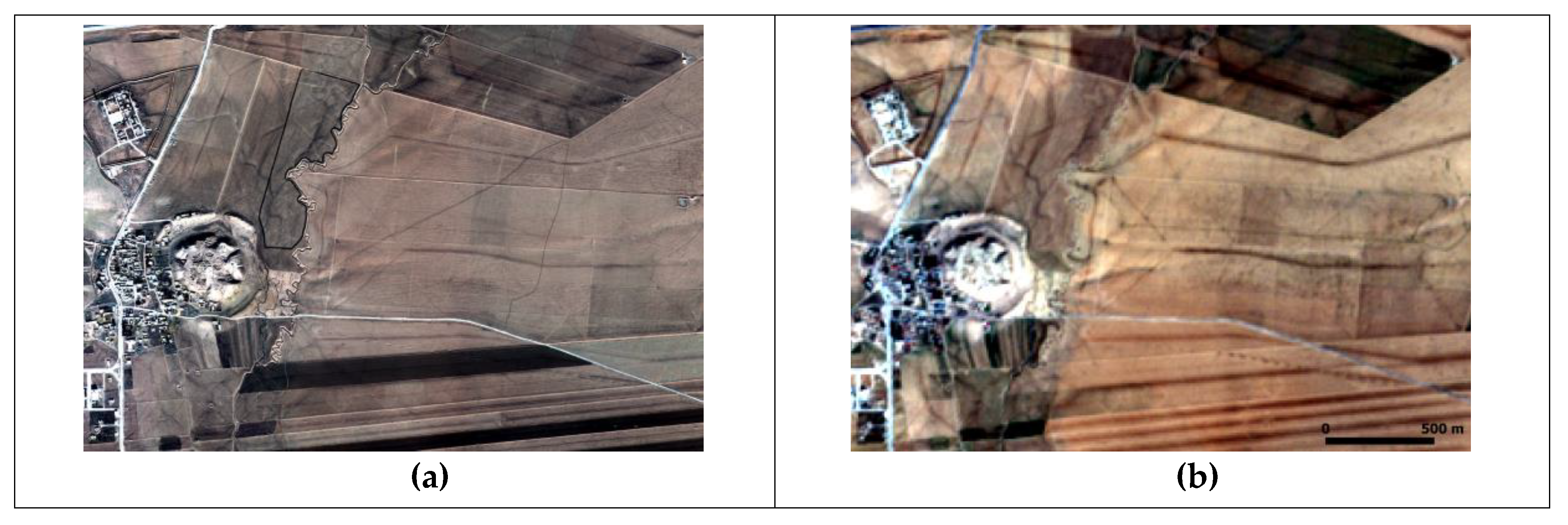
(a) Hollow ways radiating from Tell Brak (#2 on Figure 1) are clearly visible in CORONA imagery (DS1102-1025DA013, CORONA KH-4B; December 1967); (b) Landsat TM true color imagery (LT51710351990149RSA04; Landsat 5; May 1990) can also capture hollow ways, albeit to a lesser extent due to Landsat’s lower spatial resolution, but also because of the impact of the mechanized land-use practices after the 1980s on cultural material.
Figure 2.
(a) Hollow ways radiating from Tell Brak (#2 on Figure 1) are clearly visible in CORONA imagery (DS1102-1025DA013, CORONA KH-4B; December 1967); (b) Landsat TM true color imagery (LT51710351990149RSA04; Landsat 5; May 1990) can also capture hollow ways, albeit to a lesser extent due to Landsat’s lower spatial resolution, but also because of the impact of the mechanized land-use practices after the 1980s on cultural material.

Figure 3.
CORONA (DS1105-1025DA063; Nov 5, 1968) historical satellite imagery is an excellent source for mapping hollow ways with high precision. The basaltic landscape to the west of Tell Beydar (represented by the white dot at the center) does not contain evidence of movement, which may indicate differential route formation conditions or selective choices about movement.

Figure 4.
30 sample hollow ways with variable lengths superimposed on (a) averaged Normalized Difference Vegetation Index (NDVI) values for May (2014–2017) and (b) averaged Normalized Difference Water Index (NDWI) values for November (2014–2017).
Figure 4.
30 sample hollow ways with variable lengths superimposed on (a) averaged Normalized Difference Vegetation Index (NDVI) values for May (2014–2017) and (b) averaged Normalized Difference Water Index (NDWI) values for November (2014–2017).

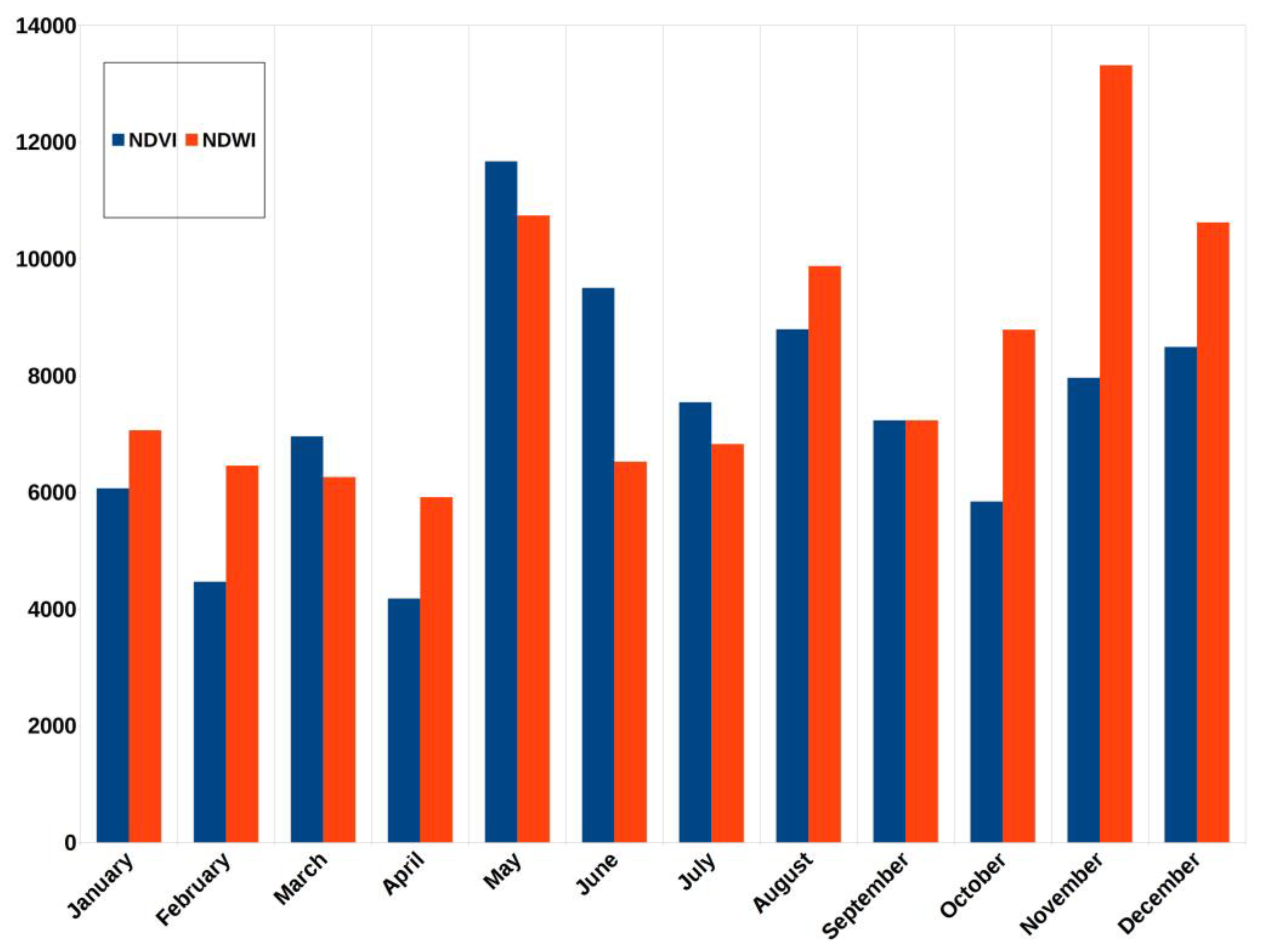
Figure 5.
The total length of digitized hollow ways is represented in the y-axis (in meters). The variation between months can be attributed to differential vegetation growth and changes in soil moisture. For this sample, the May average detected the greatest proportion of the full extents of hollow ways for NDVI (11,672 m). For NDWI the November average maximized the documentation of hollow ways (13,317 m).

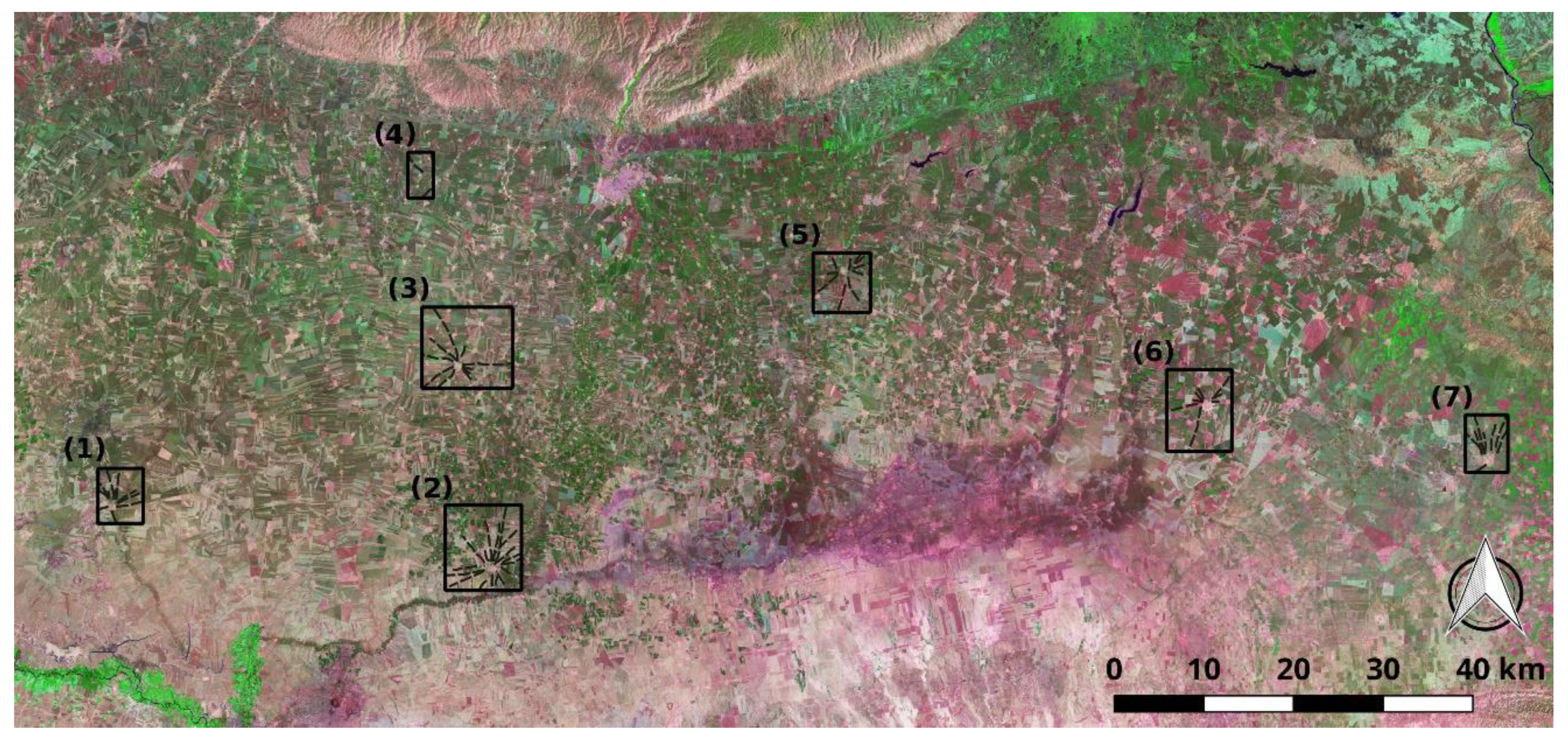
Figure 6.
Sample areas representing the hinterlands of (1) Tell Beydar; (2) Tell Brak, (3) Tell Arbid, (4) Tell Mozan, (5) Tell Leilan, (6) Tell Hamoukar, and (7) Tell al-Hawa. The base map is a True-color Landsat mosaic imagery from the USGS.
Figure 6.
Sample areas representing the hinterlands of (1) Tell Beydar; (2) Tell Brak, (3) Tell Arbid, (4) Tell Mozan, (5) Tell Leilan, (6) Tell Hamoukar, and (7) Tell al-Hawa. The base map is a True-color Landsat mosaic imagery from the USGS.

Figure 7.
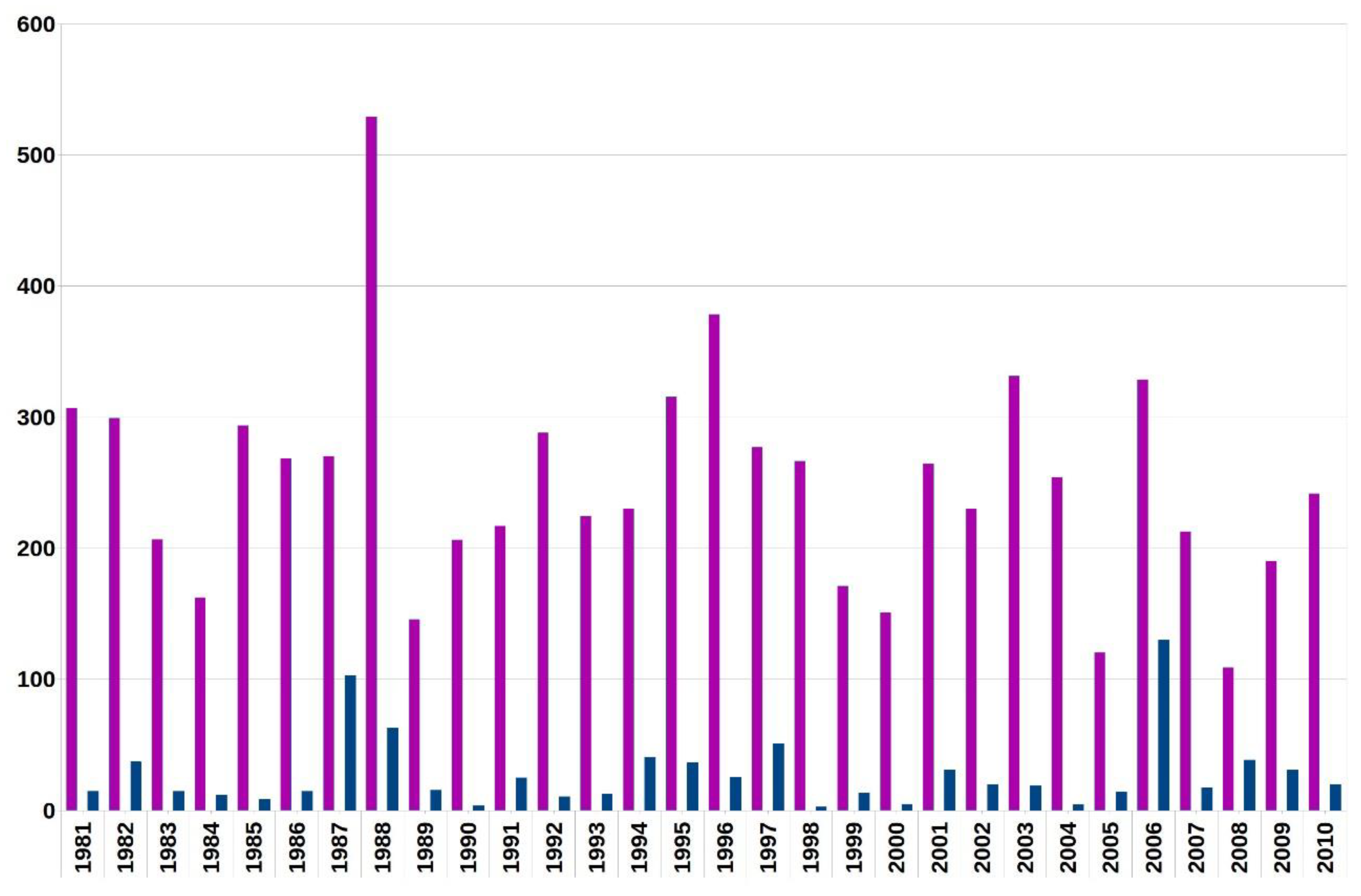
Averaged precipitation from all sample areas. Purple bars indicate accumulated precipitation values for May and blue bars for November. The wettest spring accumulation (by the end of May) was in 1988 and the wettest fall accumulation 2006 (by the end of November). The driest May accumulation was in 2008 and the driest November accumulation 1998. Other values range in between these years without an apparent trend.
Figure 7.
Averaged precipitation from all sample areas. Purple bars indicate accumulated precipitation values for May and blue bars for November. The wettest spring accumulation (by the end of May) was in 1988 and the wettest fall accumulation 2006 (by the end of November). The driest May accumulation was in 2008 and the driest November accumulation 1998. Other values range in between these years without an apparent trend.

Figure 8.
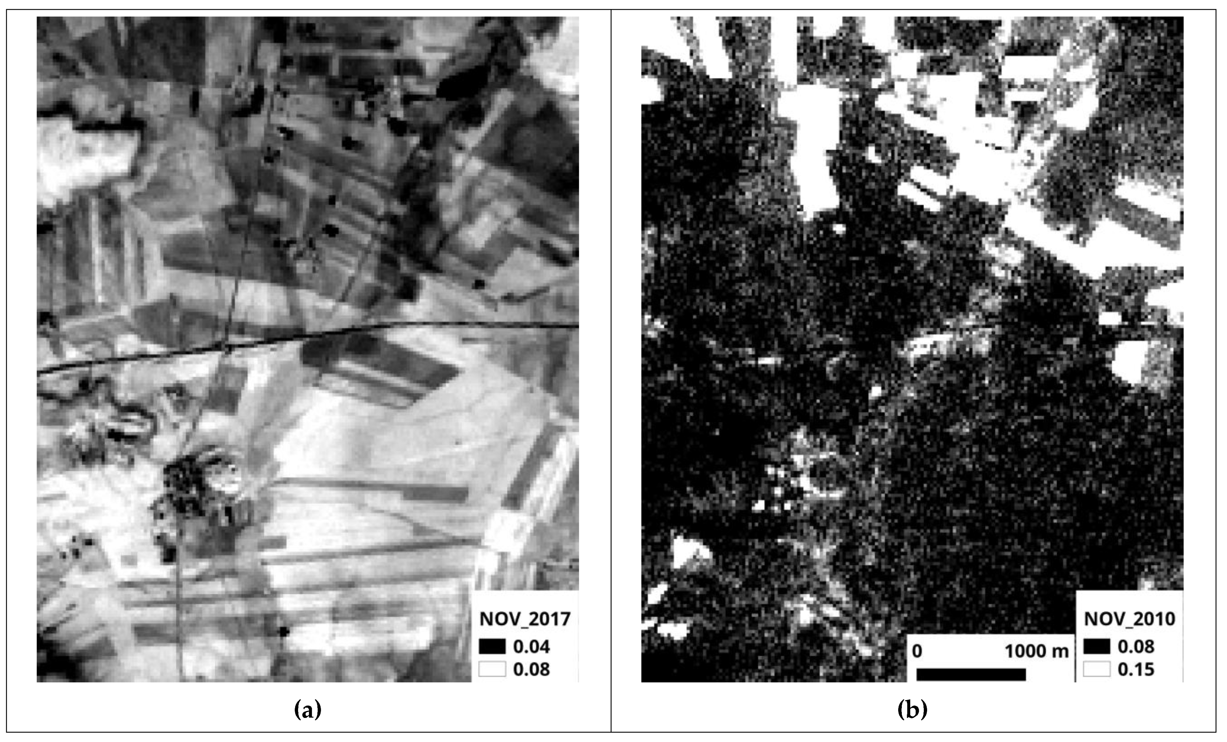
(a) NDVI values calculated from Landsat 8 for the area around Tell Beydar in November (2017) are high quality and ready for further statistical analysis; (b) Landsat 7 produces a lower-quality NDVI November dataset (2010) for the same area. Both datasets are displayed with the same rendering parameters.
Figure 8.
(a) NDVI values calculated from Landsat 8 for the area around Tell Beydar in November (2017) are high quality and ready for further statistical analysis; (b) Landsat 7 produces a lower-quality NDVI November dataset (2010) for the same area. Both datasets are displayed with the same rendering parameters.

Figure 9.
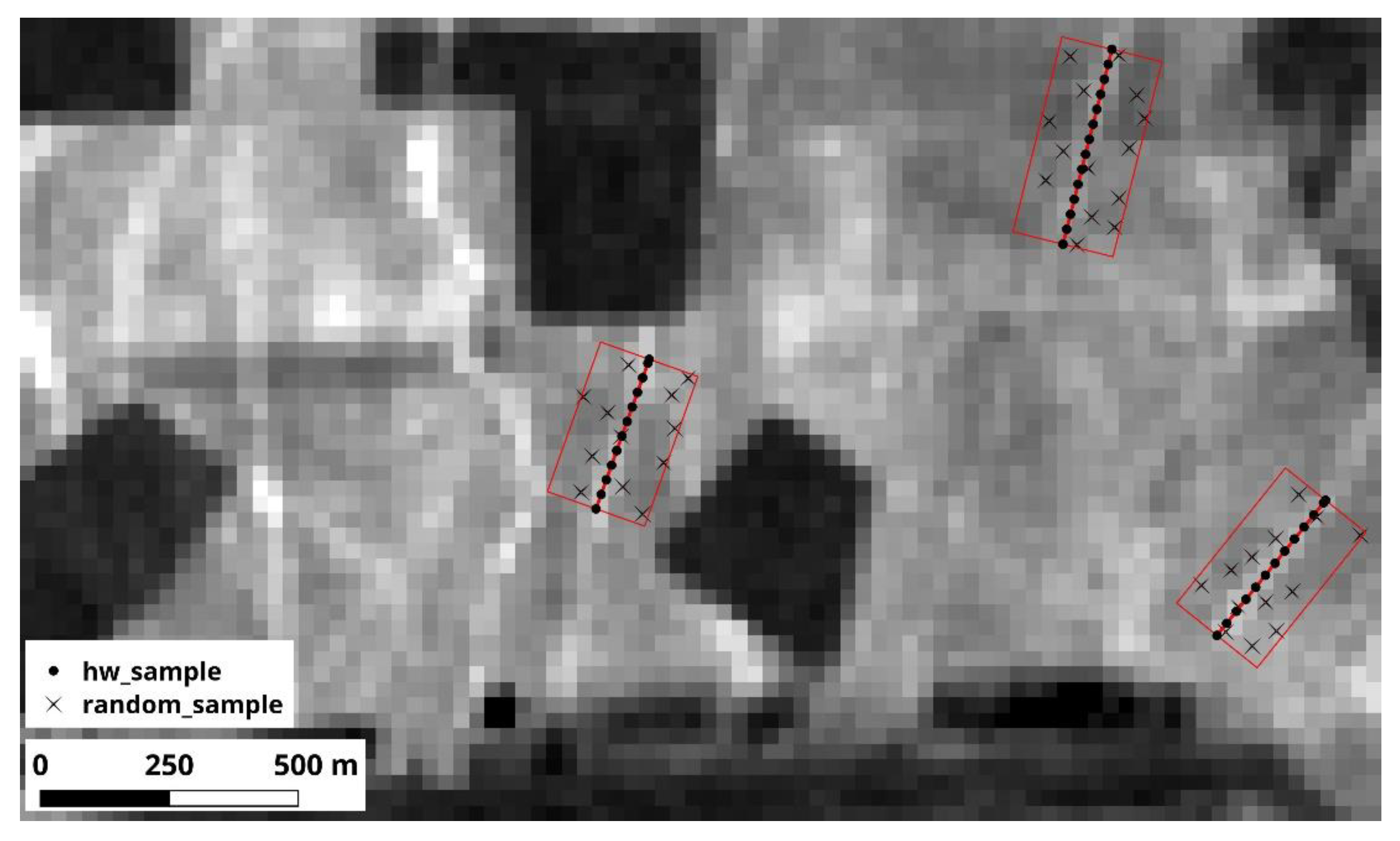
A visual representation of three hollow ways superimposed over an image of the Wetness index (WET). Buffer zones contain randomly selected background samples (stars), dynamically matching the number of systematic spectral index readings along hollow way (dots).
Figure 9.
A visual representation of three hollow ways superimposed over an image of the Wetness index (WET). Buffer zones contain randomly selected background samples (stars), dynamically matching the number of systematic spectral index readings along hollow way (dots).

Figure 10.
Monthly whisker-box plots of NDVI values of hollow ways (green) and the index values of randomly selected points from the whole scene (red). It is clear that March and April have the highest index values, and in these months hollow ways—on the average—are more separated spectrally than the background in comparison to other months. Nevertheless, more hollow ways are visible to the naked eye in May, making this a better month for mapping purposes.

Figure 11.
Monthly whisker-box plots of NDWI values. As in the case of NDVI, March and April have the highest spectral separation (green: hollow ways; red: background), but the November dataset is the most suitable for mapping due to the hollow ways being more visible to the naked eye.
Figure 11.
Monthly whisker-box plots of NDWI values. As in the case of NDVI, March and April have the highest spectral separation (green: hollow ways; red: background), but the November dataset is the most suitable for mapping due to the hollow ways being more visible to the naked eye.

Figure 12.
The Correspondence Analysis (CA) of significant indices from May.

Figure 13.
(a) Very High Resolution WorldView-3 satellite imagery (06 January 2017) still contain detailed evidence of hollow ways despite the impact of modern land-use practices on archaeological landscapes. (b) Sentinel-2 (24 February 2017) might have coarser resolution in comparison to WorldView-3, but with European Space Agency’s open-access policy, the system is a prime choice. The hollow ways still appear in great clarity on Sentinel2 Earth Observation satellites.

Table 1.
Landsat acquisition dates and respective IDs for each sample area
| Acquisition Date | Landsat ID | Sample Areas |
|---|---|---|
| 1989MAY (1989-05-10) | LT51710351989130RSA00 | 1,2 |
| LT51710341989130RSA00 | 3,4,5,6,7 | |
| 2000NOV (2000-11-08) | LE71710352000313EDC00 | 1,2 |
| LE71710342000313EDC00 | 3,4,5,6,7 | |
| 1990MAY (1990-05-29) | LT51710351990149RSA04 | 1,2 |
| LT51710341990149RSA04 | 3,4,5,6,7 | |
| 2005NOV (2005-11-14) | LT51710352005318MTI00 | 1,2 |
| LT51710342005318MTI00 | 3,4,5,6,7 | |
| 1992MAY (1992-05-26) | LT41710351992147XXX02 | 1,2 |
| LT41710341992147XXX01 | 3,4,5,6,7 | |
| 1996NOV (1996-11-05) | LT51710351996310RSA00 | 1,2 |
| LT51710341996310RSA00 | 3,4,5,6,7 | |
| 1988MAY (1988-05-23) | LT51710351988144RSA00 | 1,2 |
| LT51710341988144RSA00 | 3,4,5,6,7 | |
| 1988NOV (1988-11-15) | LT51710351988320RSA00 | 1,2 |
| LT51710341988320RSA00 | 3,4,5,6,7 |
Table 2.
Spectrally significant indices from November and the count of represented sample areas for each precipitation statistic.
Table 2.
Spectrally significant indices from November and the count of represented sample areas for each precipitation statistic.
| MIN | LOW | HIGH | MAX | SUM | |
|---|---|---|---|---|---|
| GDVI | 4 | 1 | 2 | 0 | 7 |
| MNLI | 4 | 3 | 3 | 4 | 14 |
| NDMI | 4 | 3 | 3 | 4 | 14 |
| WET | 3 | 1 | 1 | 2 | 7 |
Table 3.
Spectrally significant indices tabulated for the seven sample areas. No single index provided significant contrast for all of the areas. DWSI5 is the most optimal index, as it was able to capture contrast differences at different precipitation levels. GDVI displayed the worst performance.
Table 3.
Spectrally significant indices tabulated for the seven sample areas. No single index provided significant contrast for all of the areas. DWSI5 is the most optimal index, as it was able to capture contrast differences at different precipitation levels. GDVI displayed the worst performance.
| MIN | LOW | HIGH | MAX | SUM | MIN | LOW | HIGH | MAX | SUM | ||
|---|---|---|---|---|---|---|---|---|---|---|---|
| ARVI | 3 | 1 | 3 | 4 | 11 | MCARI | 4 | 0 | 4 | 3 | 11 |
| DVI | 3 | 1 | 4 | 3 | 11 | MNLI | 3 | 1 | 4 | 3 | 11 |
| DWSI | 4 | 5 | 3 | 4 | 16 | MVI | 4 | 2 | 3 | 4 | 13 |
| DWSI1 | 3 | 4 | 3 | 4 | 14 | NDMI | 3 | 1 | 4 | 3 | 11 |
| DWSI5 | 5 | 4 | 4 | 5 | 18 | NDVI | 5 | 3 | 3 | 4 | 15 |
| EVI | 5 | 2 | 3 | 4 | 14 | NDWI | 3 | 4 | 3 | 4 | 14 |
| GARI | 5 | 1 | 3 | 4 | 13 | OSAVI | 5 | 3 | 3 | 4 | 15 |
| GDVI | 2 | 1 | 3 | 2 | 8 | SAVI | 4 | 3 | 3 | 4 | 14 |
| GEMI | 3 | 1 | 3 | 4 | 11 | SIWSI | 3 | 4 | 3 | 4 | 14 |
| GNDVI | 3 | 4 | 3 | 4 | 14 | SR | 4 | 2 | 3 | 4 | 13 |
| GRVI | 3 | 4 | 3 | 3 | 13 | WET | 6 | 4 | 3 | 4 | 17 |
| GVI | 3 | 4 | 2 | 2 | 11 | MSI; NLI: 0 contributions | |||||
© 2019 by the authors. Licensee MDPI, Basel, Switzerland. This article is an open access article distributed under the terms and conditions of the Creative Commons Attribution (CC BY) license (http://creativecommons.org/licenses/by/4.0/).
Share and Cite
MDPI and ACS Style
Kalayci, T.; Lasaponara, R.; Wainwright, J.; Masini, N. Multispectral Contrast of Archaeological Features: A Quantitative Evaluation. Remote Sens. 2019, 11, 913. https://0-doi-org.brum.beds.ac.uk/10.3390/rs11080913
AMA Style
Kalayci T, Lasaponara R, Wainwright J, Masini N. Multispectral Contrast of Archaeological Features: A Quantitative Evaluation. Remote Sensing. 2019; 11(8):913. https://0-doi-org.brum.beds.ac.uk/10.3390/rs11080913
Chicago/Turabian StyleKalayci, Tuna, Rosa Lasaponara, John Wainwright, and Nicola Masini. 2019. "Multispectral Contrast of Archaeological Features: A Quantitative Evaluation" Remote Sensing 11, no. 8: 913. https://0-doi-org.brum.beds.ac.uk/10.3390/rs11080913
Note that from the first issue of 2016, this journal uses article numbers instead of page numbers. See further details here.