A Random Forest Machine Learning Approach for the Retrieval of Leaf Chlorophyll Content in Wheat


1
Hydrology, Agriculture and Land Observation Group, Division of Biological and Environmental Science and Engineering, King Abdullah University of Science and Technology, Thuwal 23955-6900, Saudi Arabia
2
Planet, San Francisco, CA 94107, USA
3
Kentville Research and Development Centre, Agriculture and Agri-Food Canada, 32 Main Street Kentville, Kentville, NS B4N 1J5, Canada
*
Author to whom correspondence should be addressed.
Remote Sens. 2019, 11(8), 920; https://0-doi-org.brum.beds.ac.uk/10.3390/rs11080920
Submission received: 27 February 2019
/
Revised: 2 April 2019
/
Accepted: 9 April 2019
/
Published: 16 April 2019
(This article belongs to the Special Issue Applications of Spectroscopy in Agriculture and Vegetation Research)
Abstract
:Developing rapid and non-destructive methods for chlorophyll estimation over large spatial areas is a topic of much interest, as it would provide an indirect measure of plant photosynthetic response, be useful in monitoring soil nitrogen content, and offer the capacity to assess vegetation structural and functional dynamics. Traditional methods of direct tissue analysis or the use of handheld meters, are not able to capture chlorophyll variability at anything beyond point scales, so are not particularly useful for informing decisions on plant health and status at the field scale. Examining the spectral response of plants via remote sensing has shown much promise as a means to capture variations in vegetation properties, while offering a non-destructive and scalable approach to monitoring. However, determining the optimum combination of spectra or spectral indices to inform plant response remains an active area of investigation. Here, we explore the use of a machine learning approach to enhance the estimation of leaf chlorophyll (Chlt), defined as the sum of chlorophyll a and b, from spectral reflectance data. Using an ASD FieldSpec 4 Hi-Res spectroradiometer, 2700 individual leaf hyperspectral reflectance measurements were acquired from wheat plants grown across a gradient of soil salinity and nutrient levels in a greenhouse experiment. The extractable Chlt was determined from laboratory analysis of 270 collocated samples, each composed of three leaf discs. A random forest regression algorithm was trained against these data, with input predictors based upon (1) reflectance values from 2102 bands across the 400–2500 nm spectral range; and (2) 45 established vegetation indices. As a benchmark, a standard univariate regression analysis was performed to model the relationship between measured Chlt and the selected vegetation indices. Results show that the root mean square error (RMSE) was significantly reduced when using the machine learning approach compared to standard linear regression. When exploiting the entire spectral range of individual bands as input variables, the random forest estimated Chlt with an RMSE of 5.49 µg·cm−2 and an R2 of 0.89. Model accuracy was improved when using vegetation indices as input variables, producing an RMSE ranging from 3.62 to 3.91 µg·cm−2, depending on the particular combination of indices selected. In further analysis, input predictors were ranked according to their importance level, and a step-wise reduction in the number of input features (from 45 down to 7) was performed. Implementing this resulted in no significant effect on the RMSE, and showed that much the same prediction accuracy could be obtained by a smaller subset of indices. Importantly, the random forest regression approach identified many important variables that were not good predictors according to their linear regression statistics. Overall, the research illustrates the promise in using established vegetation indices as input variables in a machine learning approach for the enhanced estimation of Chlt from hyperspectral data.
1. Introduction
Chlorophyll present in green leaves, is a key driver of photosynthesis [1,2] through its ability to convert sunlight into the biochemical energy responsible for carbon fixation. Chlorophyll works as an indirect measure of the gross primary productivity of an ecosystem [3] due to its robust relationship with vital biophysical and biochemical processes [4,5,6]. The accurate estimation of leaf chlorophyll content (Chlt) is an important element in monitoring overall plant health, managing fertilizer application, as well as other inputs in agricultural systems, where productivity levels are directly related to plant condition. Traditional laboratory-based methods of measuring photosynthetic pigments involve complex procedures of solvent extraction followed by in vitro spectrophotometric determination, which make them destructive, labor-intensive, time-consuming, and expensive [7]. Likewise, laborious sampling and analytical procedures generally make data collection over larger space and time domains impractical. As an alternative, spectral sensing has gained much attention for crop management and yield estimation over the past few years [6,8], with its application to high-throughput plant phenotyping efforts also showing considerable promise [9]. Importantly, narrowband hyperspectral measurement has the potential to offer a reliable, rapid, cost-effective, and non-destructive approach to assess the key photosynthetic pigments in leaves over a large area [10].
It is well recognized that the spectral properties of a leaf are governed by surface characteristics, internal structure, and concentration of biochemical constituents [11]. As such, many vegetation indices (VIs) have been derived from various mathematical combinations (simple ratios, differences, normalized difference, and derivatives) of hyperspectral data in order to help characterize some of these plant features. Vegetation indices constructed from data in the visible to near-infrared (VNIR) and shortwave infrared (SWIR) region of the electromagnetic spectrum have shown much value as tools for the prediction of biomass production [12], leaf biochemical constituents [13], and physiological characteristics [14]. Indeed, there are several advantages to using VIs instead of single bands, as the index normalization typically enhances the interpretability of plant properties by reducing the impact of non-photosynthetic plant elements, such as soil background, atmospheric conditions and spectral geometry [15]. Vegetation indices have been used as a tool to detect not only the spatial variability within the field, but also the seasonal variability of green foliage, making them suitable for application in precision agriculture and crop phenotyping [16].
Active research continues into the appropriate interpretation and understanding of the nature of developed VIs as optimized for particular applications [17]. Many previous studies have shown how using a single, or even a few, VIs calculated from remotely sensed data can help with estimating crop properties [12,18,19]. However, pre-selecting only a few spectral bands (out of the entirety of the VNIR spectral range) to derive a single vegetation index that measures a particular biochemical or biophysical attribute has the potential to ignore useful information contained within the remaining spectral data [20]. While in the past this has been the result of the relatively limited availability of satellite-based spectral bands, an expansion of hyperspectral capabilities, both for on-ground and remote sensing retrieval, provides new opportunities to explore the benefit of high-spectral-resolution information content [6,21].
Apart from the use of hyperspectral sensors to provide improved insight and understanding of plant behavior and response, big data analytics, in conjunction with advances in computational capacity, has opened up new avenues for the development of novel tools and techniques to extract enhanced information content. In recent years, machine-learning techniques have been employed using spectral reflectance data as input to build predictive models for plant traits, showing improved prediction accuracy and robustness [18,19]. Random Forest (RF) approaches are among the most popular machine learning methods due to their proven accuracy, stability, and ease of use. RF machine learning also provides two straightforward methods for feature selection: mean decrease impurity and mean decrease accuracy [22,23]. The random forest approach has several advantages over other machine learning techniques in terms of efficiency and accuracy for the estimation of agronomic parameters of crops, and has been used in applications ranging from forest growth monitoring and water resources assessment to wetland biomass estimation [19,24,2526,27].
To date, relatively few studies have investigated the use of VIs as input features in the RF model for the prediction of plant traits. RF-based machine learning models, using vegetation indices derived from multispectral data as input, have been used for the prediction of leaf area index [28], leaf nitrogen [20], and SPAD values [28]. Normalized difference vegetation indices (NDVIs) derived from multispectral data have also been used as input to an RF machine learner for differentiation between plant species [15]. In one study, wetland vegetation biomass was estimated by Mutanga et al. [26] using NDVI derived from WorldView-2 data as an input variable. In another, Liang et al. [29] established diagnostic models of dust stress intensity in wheat from a random forest classification algorithm using VIs (designed for dust pollution stress) as input variables. A paper relevant to the present work is that of Wang et al. [19], who determined that the RF regression algorithm was the most useful machine learning method for wheat biomass estimation, compared against a support vector regression (SVR) and an artificial neural network (ANN) implementation. In their study, 15 VIs calculated from multispectral satellite data were collected at three stages (jointing, booting and anthesis) of wheat growth, and used as input variables to the RF machine learner. Another recent and related study explored the application of a number of machine learning approaches and more than 90 vegetation indices to estimate the chlorophyll content in shaded tea [30], and found that a Kernel-based extreme learning approach performed best.
The objective of the present study was to evaluate the potential of hyperspectral data to quantify Chlt in wheat, using traditional statistical approaches in conjunction with machine learning techniques. We hypothesize that using different combinations of established vegetation indices could provide improved estimates of Chlt than using any single index alone. In exploring this idea, we also examine the retrievable information content obtained from exploiting the entire high-resolution hyperspectral dataset (2102 bands) relative to a subset of 45 established vegetation indices, using both as input predictors in a machine learner. A key objective of our study was to examine the use of these established VIs as predictors of Chlt. We benchmark the random forest machine learning techniques performance relative to that of a simple linear regression against individual indices.
2. Materials and Methods
To establish the performance of both simple regression and machine learning approaches for the prediction of Chlt from both selected vegetation indices and full-spectrum data, we devised a greenhouse-based experiment with wheat plants. The plants were grown across a number of stress gradients (nutrient and salinity) and their growth monitored throughout the crop development cycle. Details on the hyperspectral data and the experiment are provided in the following paragraphs.
2.1. Greenhouse Pot Experiment
The study was conducted at the greenhouse facility of King Abdullah University of Science and Technology using spring wheat (Triticum aestivum L.) as the selected plant material. The growing medium was a mixture of mineral soil collected from a nearby field and commercial organic soil. The field soil is classified as a calcareous alluvium Aridisol (Typic Haplargid), which is a coarse‒loamy textured, thermic, and nutrient-deficient soil [31]. The field-collected soil was air-dried, ground, and passed through a 2-mm sieve. The mineral soil was amended with a commercial organic soil-mix with a ratio of 70:30 (v/v) and placed into 2.5 L plastic pots, ensuring a bulk density of 1.2 g·cm−3 (typical of a plow layer in a cultivated field) [32]. Four seeds were sown in each pot. On the tenth day after sowing, over 90% germination was observed. The pots were then thinned to two uniformly germinated plants per pot for the remainder of the experiment. Plants were grown at a water holding capacity of nearly 70% during the experimental period through a regulated irrigation in which water lost from a pot via evapotranspiration was replenished with fresh non-saline irrigation water. The water lost was measured as the difference between weights of each pot between two irrigation time intervals. The experiment was maintained and monitored over the entire growth cycle of approximately 120 days until harvest.
2.2. Hyperspectral Data Acquisition
Hyperspectral measurements and sample collection for laboratory determination of Chlt were undertaken within two days at the anthesis stage. This period is known as the lag phase, during which cellular division is rapid and endosperm cells and amyloplasts are formed, and is considered very sensitive to environmental stresses [33]. Starting next to the flag leaf, five leaves were selected from the top to the bottom of the plant, so that sampling covered leaves of all ages on the plant. Leaf hyperspectral measurements were collected using a full-range hyperspectral ASD FieldSpec 4 Hi-Res (Analytical Spectral Devices Inc., Boulder, CO, USA) spectroradiometer. The FieldSpec collects data in the 350–2500 nm spectral range, with a resampled spectral resolution of 1 nm. The spectral resolution in the visible-to-near infrared (VNIR) is 3 nm, while the shortwave infrared (SWIR) is 8 nm. Leaf spectral reflectance was measured using the leaf contact probe of the ASD, with 10 spectral measurement taken on each leaf. The contact probe has a diameter of 25 mm, an instantaneous field of view (FOV) of 10 mm, as well as its own halogen lamp as the internal light source. During a preliminary experiment, we observed that more than a few seconds’ exposure to the internal light of the contact probe caused leaf damage. We also observed that direct clamping on attached leaves resulted in condensation of vapor on the lens, which could result in erroneous readings and spectral noises at the water absorption bands of the leaf spectra. In addition, wheat leaves are narrower than the field of view of the FieldSpec’s leaf probe. Therefore, we modified the clamping part of the contact probe to confine the exposure area of leaf. We tested a few options for this purpose, with improved results achieved by making a rectangular hole of 0.9 × 1.5 cm−2 in the black gasket of the LiCOR fluorometer chamber and using this as a mask in the leaf probe. These gaskets do not reflect the incoming radiation form the probe light sources. Prior to plant spectral measurement, a so-called white reading was taken using a Spectralon reference panel in the probe. This measurement determines the spectral response from a surface with close to 100% reflectivity. Leaf reflectance was computed as the ratio of leaf radiances relative to the radiance from the white reference panel. The calibration with the Spectralon was repeated every 30 min during the measurement process. For every point of measurement, 10 spectral measurements were recorded from the adaxial leaf surface against the dark background of the probe. Considering that there were 27 different salinity and nutrient treatments being explored, with two plants grown per plot, the total number of spectral measurements amounted to 2700 for the entire experiment (i.e., 2 plants per plot × 27 treatments × 5 leaves per plant × 10 measurements per leaf).
2.3. Chlorophyll Determination
Leaf Chlt was determined by collecting samples from the point leaves (and corresponding to the spectral sampling) via chemical extraction and spectrophotometric analysis in the laboratory. Each sample was composed of three leaf discs punched from the same location on the leaf that the spectral data were sampled. As such, a total of 270 samples were collected across the gradients of soil salinity and fertilizer treatment. A paper punch was used to collect leaf discs of 7 mm diameter (area = 0.38 cm2). From each sampling point, three discs (A = 1.14 cm2) were placed in Eppendorf tubes and immediately wrapped in aluminum foil and then stored in ice. All samples were labeled on the top and side of the Eppendorf tube, with a corresponding label of plant and treatment recorded in a notebook. Samples were transported to the laboratory within 30 min of collection and stored at −80 °C till further analysis. Pigment contents were determined using the methods of Arnon [34] and Wellburn [35]. Briefly, the samples were ground in liquid nitrogen using the SPEX Sample Prep TM CryoStation (2600) and Geno/Grinder. The ground samples were extracted in 80% acetone at room temperature after centrifugation. Pigment absorption contents were then measured spectrophotometrically at 663, 645, and 470 nm using an Infinite M1000 PRO plate reader, and translated into pigment contents calculated using the following equations from Arnon [34] and Wellburn [35]:
where Chla is the chlorophyll-a content, Chlb is the chlorophyll-b content, Ct is the carotenoids content (all in units of and Aλ is the absorbance at wavelength λ (nm).
2.4. Hyperspectral Data Processing and Extraction of Vegetation Indices
Spectral bands ranging from 350 to 400 nm were removed due to the considerable signal noise in that region. Our approach was to investigate the impact of using bands distributed across the entire spectral range (400–2500 nm) versus a selection of distinct vegetation indices, using both of these datasets as model input parameters for estimating leaf Chlt. A database of 45 vegetation indices (Table 1), which have shown potential for assessing attributes of vegetation parameters related to plant phenology and biochemistry, were preselected for analysis. Constituent bands of the vegetation indices were first calculated from the high resolution hyperspectral data by taking the average of the b ± 2 bands, where b represents the band center. This allowed us to make use of the neighboring wavelengths of the target bands in the high-resolution data. The list of indices in Table 1 includes 15 vegetation indices that were calculated based on the first derivative of the spectral data in the visible red-edge region. These indices, referred to as Derivative Normalized Difference (DND) measures, are normalized difference indices of the first derivative of the transformed narrow-bands [36] determined at various reflectance band combinations. For example, the red-edge position of the reflectance spectra is defined by the maximum first derivative of the wavelengths in that region [18,37] (i.e., the maximum slope across the spectral measurements in that range). The red-edge position and the variations in the relative heights of the maxima in the first derivative of the red-edge region are induced by alterations in the leaf pigments, due to biotic or abiotic factors. Indices from the first derivatives of the reflectance spectra at 650–750 nm, have previously been used for estimation of chlorophyll related vegetation characteristics [18,36,38]. Normalized difference indices of the first derivative can be determined at various reflectance band combinations. The first derivative Dλ can be calculated as (Dλ+10 − Dλ−10)/20, where λ represent the specific reflectance band. Such indices have shown resistance to background contributors (such as soil), which are responsible for distortions in the reflectance spectra [39] and have demonstrated applications related to chlorophyll-based characteristics of vegetation in several areas [18]. All of the data processing and calculations of the VIs were performed in the MATLAB (MathWorks, Inc., Natick, MA, USA) software package.
2.5. Statistical Analysis and Machine Learning
Three distinct procedures were undertaken to establish the relative capacity to retrieve Chlt using hyperspectral data. In the first, simple linear regression of the Chlt against the 45 unique vegetation indices calculated from the hyperspectral data was employed. Following this, an implementation of a random forest machine learning approach was used to examine: (1) the full range of the hyperspectral data, using individual bands as input variables to monitor pigment retrieval; and (2) the use of established vegetation indices as input variables to infer Chlt, initially using the 45 selected indices and then progressively reducing the number of input variables to observe the impact on retrieval accuracy. The MATLAB (MathWorks, Inc., Natick, MA, USA) software platform was used for both the data analysis and the implementation of the machine learning algorithm. Following is a more detailed description of each of these procedures and the underlying rationale used.
2.5.1. Simple Univariate Regression Analysis
The indices in Table 1 were evaluated for their performance in estimating leaf Chlt by undertaking simple regression analysis and curve fitting on the data obtained from laboratory analysis of leaf samples and the in situ collected spectral data. During the analysis, each of the VIs were used as a single explanatory variable one-by-one for estimation of Chlt. Several regression models including linear, quadratic, logarithmic, cubic, exponential, inverse and power were examined, and the best-performing models were chosen based on the coefficient of determination (R2) and the root mean square error (RMSE). While regression analysis is simple to implement, fast to model, and particularly useful when the variable space is not particularly complex, other more advanced data analytics are likely required to fully exploit highly complex and multi-dimensional hyperspectral datasets.
2.5.2. Description of the Random Forest Approach
Spectral datasets typically contain many more unique variables than the physical measurements against which they are compared. Taking advantage of the large number of narrowband high resolution spectral data with corresponding pigment data, we also explored the performance and accuracy of predicting Chlt from spectral data via a multivariate regression analysis (i.e., the random forest machine learning approach). The rationale for doing this is the inability of general linear models to relate the large number of explanatory variables (narrow spectral bands and VIs) that interact to provide an accurate representation of a response variable (in this case chlorophyll). RF is a non-parametric ensemble classification and regression machine learning approach based on many decision trees as base classifiers [22,23,24]. It provides a means of averaging predictions of multiple decision trees, trained on different subsets of the same data in order to overcome the problem of over-fitting by individual decision trees. While there are many potential machine learning approaches that could be employed [23,25,30], the RF approach has been shown to provide relatively good accuracy without the danger of overfitting. The bootstrapping approach, representing the random selection of a subset sampled from the entire dataset that is used in the construction of decision trees, also acts to reduce the prediction error [24]. Instead of growing a single deep decision tree, growing multiple trees with parallelized computations also makes the algorithm quite fast. In addition, the RF machine learning method provides a straightforward approach of feature selection and of cascading the variable importance. There are relatively few assumptions attached to RF, so data preparation and model parameterization is less challenging.
To understand how the RF works first requires an understanding of what decision trees are and how they are grown. Decision trees (named after the tree-like structure representation of the predictive model) are statistical models designed for supervised prediction problems in which a set of explanatory variables (also known as input features or predictors, i.e., spectral bands and VIs in our study) are used to predict the value of a response or target variable (e.g., Chlt). An illustration of a simple decision tree analysis is provided in Figure 1. Here the tree is read from the top down, starting from the root (root node), going down through the internal nodes (the splits based on the values of one of the predictors), and finishing when a terminal node (called a leaf) is reached. Each regression tree extends from the roots to leaves under a set of conditions and restrictions [22]. The internal nodes are decision points. The starting point of the single decision tree growth is to draw several bootstrap samples (randomly selected subset data) from the larger training dataset. This increases diversity in the forest, leading to a more robust overall prediction. A regression tree is fitted to each of the bootstrap samples in such a way that for each node of a tree, a subset of randomly selected input predictors is considered for binary partitioning (a binary decision rule is applied for split at each node). The Gini Index is often used for split based on a pure choice in the decision trees (choosing the input predictor with the lowest Gini Index):
where xi is a value of the sample proportion, is the proportion of samples with the value xi belonging to leaf j at node t [19]. Each decision tree grows from the root node, splits into branches (intermediate nodes) and down to terminal nodes (leaves). Every node in the tree checks a condition of only one predictor variable at a time (e.g., NDVI < 0.5) for all the observations. If the condition is fulfilled, another predictor variable is taken for the next node (e.g., SAVI < 0.7) and a decision is made in a binary fashion. In this way, the decision tree grows down to terminal nodes (leaves) and each leaf contains a response. Two inputs are required to be optimized at the beginning of the RF implementation. The first is the number of regression trees (ntree) needing to be at maximum for a dense forest. The second is the “number of leaves,” which corresponds to the terminal nodes of the tree (i.e., tree growth is stopped). Too large a number of leaves means stopping tree growth after only a few splits (shallow trees), which could result in poor predictive performance. On other hand, a small number of leaves (deep trees) could result in overfitting [62]. Predictive power is calculated based on an aggregate from all the trees.
Each tree of the random forest is constructed based on a different model. The bootstrapping samples randomly selected from the total are called “in bag” samples, while those not used in the model construction are referred to as “out of bag” (oob) samples. This concept gives random forest the power of not needing a separate set of data for model evaluation, i.e., the prediction error is measured through an out-of-bag error method in the RF and independent cross-validation is not necessarily required. Typically, two-thirds of the samples are used for model training and one-third of the samples are used as oob samples. Oob estimates provide RF with robust measures of model accuracy, as the oob samples are not used for building the trees. Thus, overall model accuracy results from aggregating oob-based predictions over all the trees. In our study, the model accuracy was assessed via the RMSE.
2.5.3. Implementing the Random Forest Approach
Before using established VIs as input features into the leaf chlorophyll prediction model, we first trained the model using all of the individual spectral bands (i.e., 2102 bands in total) as input features. Responses from all the predictors were recorded and statistical parameters (R2 and RMSE) were calculated. In a second experiment, we retrained the model using the established VIs as input features and examined the difference between the results. The modeling procedure was performed as follows:
- Define the optimum number of trees (ntree) based on a bootstrapping sampling procedure.
- Optimal number of leaves (nodesize) was decided as a specified stop condition to reach during the data splitting process at all internal nodes. Leaves are the terminal nodes where the tree growth is stopped. If the trees are allowed to grow to full depth, it may be too variable (i.e., result in relatively high variance and low bias and a possible overfitting of the data). Thus, pruning of the tree is done by deciding upon the optimal number of leaves.
- At every node of the tree, the number of input variables (mtry) (i.e., number of individual bands or VIs) used for the split decisions were randomly selected out of the total (2102 individual spectral bands or 45 VIs).
- The stop condition of each tree growth in our method was determined by defining an optimum number of leaves. The number of trees and number of leaves were optimized by minimizing the RMSE. A diagram of the workflow is provided in Figure 2.
The relative importance of the input features was measured at the completion of the RF model training. The variable importance is based on the concept that if the exclusion of a variable is associated with a considerable reduction in prediction accuracy, then that variable is deemed as important. Thus, a subset of attributes is selected based on the importance scores. The procedure adopted in this study is referred to as the “permutation accuracy importance,” and is considered one of the more useful approaches for ranking variable importance [22,63]. The procedure is carried out in two steps to simplify the RF model without losing predictive accuracy. In the first step, the model is trained using all of the predictors as input features. The aim of the second step is to determine the effect on model performance by progressively reducing the number of predictors using an iterative elimination of the less important predictors to determine the predictive accuracy of the RF model [64]. Based on this rule, the number of input features (VIs) were reduced, step-by-step, to 50% of the total at each iteration, with this continuing until the error did not increase significantly.
A typical benchmark dataset for cross-validation consists of a training dataset and a testing dataset, but partitioning of data into two sets reduces the amount of data that can be used for training the model. The K-fold cross-validation [65] method does not involve exclusive training and validation sets. Instead of dividing the data into distinct portions, the procedure involves splitting the dataset into K number of folds, and then going through an iterative process where it first trains on the random subset size (K−1)/K of the observations (K−1 of the folds) and then evaluates performance on the random subset size 1/K of the observations (Kth fold). The process is repeated K times. At the end of the K-fold cross-validation, the average of the validation metrics for each of the K iterations is used as the final performance metric. Although out-of-bag performance for an RF model is very similar to cross-validation, it is strongly recommended to use a proper validation using an independent test dataset [66]. We first randomly split the entire dataset into two parts, a training set (80%) and a test set (20%). In this study, a 5-fold internal cross-validation method was employed to examine the predictive accuracy of the model. This implies that 80% of the training dataset was used for model training, and the remaining 20% for testing at each iteration, i.e., all of the training data are used for both training and validation after the five iterations. The R2 and RMSE presented here are the average of the five repetitions.
3. Results
3.1. Regression Analysis Using Established Vegetation Indices for Chlt Estimation
To understand whether the established vegetation indices were able to accurately estimate the Chlt in wheat leaves, we performed regression between each of the indices and the Chlt per leaf area obtained from the laboratory analysis. Traditionally, vegetation properties have been estimated using simple vegetation index relationships that are often established statistically by fitting standard regression functions based on the in situ measurements [5,23]. After evaluating various types of linear regression models, the best models were chosen for each index and accuracy parameters were recorded. The vegetation indices achieving the best fits (in terms of R2 and RMSE) are provided in Table 2 and ranked based on performance.
As can be seen, the prediction performances of the studied VIs were quite variable, with the R2 value ranging from 0.01 to 0.86 and RMSE ranging from 6.05 to 16.30 µg cm−2. The best-performing VI was found to be D12, a non-specific vegetation index presented as the simple ratio of the first derivative of the 712 to 702 nm spectral bandwidth. The R2 and RMSE for the D12 index was 0.86 and 6.05, respectively, which was followed closely by the MERIS (Medium Resolution Imaging Spectrometer) Terrestrial Chlorophyll Index (MTCI) (R2 = 0.86; RMSE = 6.07). The poorest performing index was DND6, another non-specific vegetation index, with an R2 of 0.01 and a RMSE of 16.30 µg·cm−2. The statistical ranking in Table 2 showed that the top 11 indices were largely indistinguishable, with only slight differences in R2 and RMSE values. These 11 indices adopt different combinations of two or more spectral bands sourced predominantly from the red-edge region (see Table 1) (e.g., 529, 661, 691, 702, 712, 722, 732, 742, 752, and 872 nm).
The VIs derived from the first derivatives of the spectral data (such as D12, D02, DND1, and DND8), and which were developed for quantifying overall vegetation health, tended to perform as well as (or better than) some indices specifically developed for chlorophyll estimation. Indeed, half of the indices with an R2 value above 0.80 and RMSE less than 7 µg·cm−2 (i.e., the top 16) were based on derivative calculations. The use of derivatives of specific reflectance spectra has previously been recognized as a means to eliminate the background signals (such as soil) and resolving problems related to overlapping spectral features [39]. However, due to the lack of dedicated hyperspectral sensors on satellite monitoring systems, they are not widely implemented. The strong performance of the derivative-based indices highlights the importance of an appropriate transformation of spectral data for our modeling purposes. More importantly, the results suggest the potential of using full spectrum data to enhance the detection of the target trait (i.e., chlorophyll) so that “hidden” information can be utilized.
The top four performing VIs from Table 2 were further examined in Figure 3. Following D12, the MTCI was the next best performing, with only a small difference in RMSE separating it from D12. MTCI estimates the relative position of the red-edge by using data in three wavebands centered at 681.25, 708.75, and 753.75 nm [51], is easy to calculate and is sensitive to a wide range of Chlt [50]. As can be seen in Figure 3, fitting a second-order polynomial curve to the data resulted in a high R2 (0.86) and low RMSE (6.07 µg·cm−2). The third and fourth best performing indices were the Vogelmann red-edge indices VREI1 and VREI2 [61], with an R2 of 0.85 and a RSME of 6.24 and 6.25 µg·cm−2, respectively. Both VREI1 and VREI2 are calculated from spectral bands in the red-edge region (Table 1), further establishing the importance of that portion of the spectrum. Multiple regression analysis of the four best-performing indices (D12, MTCI, VREI1, and VREI2) produced the following equation:
with an R2 of 0.86 and a RMSE of 6.04 µg·cm−2. The use of multiple regression did not improve prediction performance in terms of R2 and RMSE values. Overall, the results show that there are many vegetation indices that are able to provide a strong relationship with the Chlt in wheat leaves. However, an investigation of the full spectral range using the RF technique will provide the capacity to exploit the spectral information lie in the bands not covered by the VIs for the prediction of chlorophyll content.
3.2. RF Machine Learning Approach Using All Hyperspectral Bands as Input Features
To examine the synergistic information content available within the hyperspectral data, the RF model was trained and run using the full suite of hyperspectral bands as input features for the prediction of Chlt. The results of the RF model training, showing Chlt predicted from the model as a function of the true Chlt determined via laboratory analysis, are presented in Figure 4. Model performance was evaluated by plotting the values of actual Chlt against the Chlt predicted from the model. As can be seen in Figure 4A, the RF model fits the testing data quite well when all the spectral bands were used as input features. The R2 value of 0.89 is higher than the best-performing vegetation index achieved using simple regression analysis (0.86; see Table 2), while the RMSE was also improved (5.49 µg·cm−2) compared to that from the simple regression against the individual indices (6.05 µg·cm−2). Although the RF model shows a significantly better performance in prediction of Chlt when all the spectral bands were used input predictors, a selection of optimal input variables is consider a key feature of the RF modeling approach, which is explored in Section 3.3.
3.3. Random Forest Approach Using Vegetation Indices as Input Features
Typically, RF models are utilized as “black boxes,” the reason being that the forests contain a huge number of dense trees, and every tree is trained on bagged data based on a random selection of input features comprised of a wide range of spectral bands. This makes it infeasible to fully understand the decision process by evaluating every single tree individually. Thus, the selection of proper input parameters is a key element that is required to produce meaningful outputs. To explore this concept, the 45 selected vegetation indices from Table 1 were used as input features to train the RF model and then to predict chlorophyll. The use of vegetation indices is expected to have several advantages over utilizing the full spectrum, including reducing any redundancy in the spectral data, focusing on indices that enhance the spectral properties of vegetation, reducing any influence of background spectral noise, and simplifying the model by reducing the amount of data used.
Our results confirmed that model performance was significantly improved when the VIs were used as input predictors. The R2 value of 0.95 (see Figure 4B) is higher than the value (0.89) obtained using the RF model with all the spectral bands as input predictors. Similarly, the RMSE obtained by employing the RF model with VIs as input predicators was also much improved (3.71 µg·cm−2) compared to using all the spectral bands as input predictors (~5.49 µg·cm−2).
3.3.1. Optimization of the Random Forest Model
As noted earlier, one of the key steps in the RF machine learning implementation is the optimization of input parameters: in particular, the choice of an optimal number of trees (ntree), minimum size of terminal nodes (number of leaves, nodesize) and the number of predictors evaluated at each node (mtry), i.e., the number of random predictors selected for split [27]. The optimization of parameters was carried out under a combination of different numbers of trees and leaves in order to develop an optimal predictive model with the lowest root mean square error. We trained the model using different numbers of trees (1, 5, 10, 15, 20, 30, 60, 90, and 120) and at 1, 5, 10, and 20 leaves, aiming to identify the lowest possible number of trees and highest possible number of leaves (less dense forest with deeper trees) that generates the lowest error. Figure 5 summarizes the simultaneous evaluation of RMSE for the number of trees and number of leaves tested using all the variables under analysis.
The effect of the number of trees is evident from Figure 5A, which shows that as the number of trees increases, the RMSE decreases under all of the examined number of leaves. The decrease in error is sharper at the beginning, and then tapers off between ntree = 20 to 60. Although, our results showed that variations in RMSE are small beyond ntree = 60, we chose 120 trees for training our models, since a search of the literature has reported that RF models with ntree > 100 showed greater stability [24]. The specification of ntree will also depend on the size of the dataset, but the RF machine learning methodology can handle large numbers of trees due to the high computational efficiency and low risk of overfitting. As can be seen from Figure 5B, the lowest error was produced by the models trained with between one and five leaves. An increasing number of leaves at a given number of trees results in a higher value of RMSE. However, the difference between the RMSE values is quite low for numbers of leaves between 1 and 5. A deep tree with many leaves is usually highly accurate on the training data, as there is a tendency of overfitting by employing very leafy trees. On the other hand, a very simple tree with fewer leaves does not generally attain high training accuracy, since the training samples used to calculate the response of each leaf node is low. As such, it is important to define a balanced number of leaves that retrieve an accurate but flexible model. Following the methodology reported in related studies [62,67], we use five leaves in combination with 120 trees to train the RF model for subsequent analysis.
3.3.2. Selective Reduction of Important Predictors
Once the RF model was optimized using the selected input features (i.e., the 45 vegetation indices), they were ranked based on their importance using a forward selection function to identify which vegetation index predicts Chlt with the greatest accuracy. The model was initially applied to the training data containing all 45 vegetation indices, with Figure 6A showing the ranking of the most important vegetation indices based on out-of-bag permuted predictor estimates. Results show that the most important predictor was the Anthocyanin Reflectance Index (ARI2), followed by the Normalized Difference Water Index (NDWI), the Modified Chlorophyll Absorption Ratio Index (MCARI2), the Carotenoids Reflectance Index (CRI2) and the Structure Intensive Pigment (SIPI).
After the model evaluation using the entire set of vegetation indices as input features, subsequent iteration of the model was performed by excluding features (i.e., vegetation indices) that were identified as being the least important. At each iteration, the number of predictors were reduced by half the original number. Essentially, the least important variables were excluded and a reduced configuration was defined. Figure 6B‒D illustrates the output of the iterative procedure of permutation accuracy importance for a reduced number of important feature selections, showing the associated (minimal) impact on the RMSE. By halving the input predictors to 23, RMSE decreased from 3.75 µg·cm−2 (with 45 vegetation indices as input predictors) to 3.66 µg·cm−2 (Figure 6B). RMSE further decreased to 3.58 µg·cm−2 by reducing the number of vegetation indices input predictors to 12 (Figure 6C). However, further reduction to seven input predictors (Figure 6D) slightly increased the RMSE to 3.7. µg·cm−2. Applying the procedure across four iterations (i.e., reducing from 45, 23, 12, and then 7) we identified the seven most important vegetation indices out of the original 45 (Figure 6D). According to this analysis, the most important predictors of leaf Chlt were DND2, NDWI, DND5, PRI4, ARI2, CRI, and CRI2 (see Figure 6D), ranked in descending order of variable importance. Importantly, the top 10 best-performing VIs established from the simple linear regression (see Table 2) did not appear in the important variables identified from the RF machine learning algorithm shown in Figure 6D. Indeed, the top seven important variables resulting from the RF approach occupy the 14th, 43rd, 44th, 33rd, 32nd, 30th, and 37th places, respectively, in the ranking list based on a simple regression against the VIs (see Table 2).
One interesting outcome from this analysis is that the importance rankings, or at least the order of the ranked indices, were not always consistent throughout the iterations (see Figure 6). The values, as well as the ranked position of the different predictors, changed during repeated runs of the prediction model. Figure 7 shows the effect of repeatedly running the predictive model on the relative importance of features for the case where 15 indices were being considered as an example. The feature importance procedure was repeated 10 times to assess the ranking frequency of each importance variable, with the ranked histogram of the variable importance for the 15 most important vegetation indices provided in Figure 7A. Results indicate that ARI2 and NDWI proved to be the most important vegetation indices for prediction of Chlt when the procedure was repeated 10 times, followed by PRI4 and DND5 and CRI2. Importantly, the RMSE resulting from running the model iteratively did not change significantly. Indeed, the RMSE ranged from 3.62 to 3.91 across the different runs, with an average value of 3.76 µg·cm−2.
4. Discussion
In this study, we investigated leaf level hyperspectral data for the purpose of estimating leaf Chlt in wheat plants. Regressions analysis using established vegetation indices was explored, together with an application of a Random Forest machine learning approach, using (1) all of the available spectral bands, and (2) selected vegetation indices as predictor variables. Overall, results illustrate that the RF approach provides an improved level of retrieval accuracy relative to simple linear regression when all the spectral bands were used input predictors. The RF model performance was further improved by using an optimal number of input predictors (i.e., the 45 VIs) compared to the use of the all spectral bands input predictors for prediction of Chlt. By employing the variable importance feature of the RF modeling approach, the iterative selection of key indices showed further enhancing results. A further discussion of the elements of this analysis is presented below.
4.1. Simple Regression Analysis of the Vegetation Indices for Chlt Determination
Regression analyses examining the relationship between individual VIs and Chlt was performed, with the indices arranged in descending order of performance (as presented in Table 2). The D12 index, representing the simple ratio of the first derivative at spectral bands 712 and 702 nm, was the best-performing vegetation index based on R2 and RMSE values (0.86 and 6.05). The results are supported by earlier work such as Kochubey and Kazantsev [39], who reported a similar index (D725/D702) to accurately describe chlorophyll-related vegetation characteristics. However, the first 10 indices in Table 2 performed almost equally well, particularly with regards to their R2 (0.85‒0.86), but also their RMSE values (6.05–6.45 µg cm−2). The top-ranked list includes indices derived from a range of spectral combinations spanning the visible to red-edge portion of the electromagnetic spectrum, further verifying the sensitivity of this spectral region to Chlt [20,23,40,50].
In addition to identifying some of the vegetation indices explicitly developed for chlorophyll estimation (such as MTCI, MRENDVI, and NDRSR), indices based upon the first derivatives of the reflectance spectra occupy the highest ranks of the best-performing VIs. The various advantages of derivative-based vegetation indices over traditional simple reflectance-based indices have been reported in previous studies [38,39]. They are indicative of the slope of the reflectance spectra with respect to central band wavelength. As such, they are becoming increasingly popular, especially with the introduction of narrow band hyperspectral sensors for remote sensing [68].
Although many of the VIs under investigation performed well in determining leaf Chlt from spectral data, others illustrated poorer performance. These included indices that have previously been demonstrated to show good performance in inferring vegetation health and function. For instance, NDVI, which is routinely employed as an indicator of plant health, presented relatively poor statistical results (R2 = 0.37, RMSE = 13.0) and ranked 26th out of all the VIs tested (see Table 2). Similarly, another standard index that has been used to describe leaf area index (MCARI2 [48]), also showed a poor statistical response (R2 = 0.20, RMSE = 14.6 µg cm−2). Of course, this is not necessarily unexpected, since VIs relate most strongly to the crop type, vegetation parameter or phenological stage for which the index was developed [69], and may not be transferable to other varieties or conditions.
While hyperspectral reflectance tools offer much promise for sensing a diverse range of vegetation traits [6], systems remain expensive, require considerable computational effort to process, and in practical applications, may provide far more information than the user requires for a particular purpose. Undertaking analyses such as those performed here, allows for the identification of useful spectral combinations for specific variables of interest. So, instead of needing a hyperspectral sensor to retrieve multiple indices (that may or may not be informative), pre-defined band combinations can be incorporated into customized multispectral systems, focusing on those band combinations that are known to perform well. A number of such sensing systems are commercially available [70,71].
4.2. RF Machine Learning Approach Using Hyperspectral Bands and VIs as Input Features
The objective of employing an advanced RF machine learning technique was to make the best use of the acquired high resolution (narrowband) spectral data over a wide spectral domain, instead of using traditional approaches of selecting only a few bands out of the available high resolution data. To explore this concept, an RF (K-fold cross-validation) approach that utilized 80% of the available hyperspectral measurements as input training data and 20% as evaluation data was employed. In this iterative process, all of the data are used for both training and validation after the five iterations. First, the RF model was trained and run with the full range of hyperspectral bands as input features for the prediction of Chlt from the spectral data. In a follow-up experiment, selected VIs were used as input features to train and run the RF model for a comparative analysis. In the first experiment (as shown in Section 3.2), using all of the available spectral bands as input variables in the RF yielded improved accuracies compared to those obtained via simple regression of individual vegetation indices alone (Table 2 and Figure 3). By analyzing the estimated versus measured values (Figure 3) the RF model had significantly higher R2 (0.89) and lower RMSE values (5.49 µg cm−2) than any of the best-performing single vegetation indices. The RF model performance further improved (average RMSE = 3.76) when the 45 selected vegetation indices from Table 1 were used as input predictors to train the model for prediction Chlt. The R2 value increased to 0.95, which is higher than the value (0.89) obtained from the analysis using all the spectral bands as input predictors. Similarly, the RMSE obtained from Vis-based RF modeling was also improved (3.71 µg·cm−2) compared to that from RF model with all the spectral bands as input predictors (~5.49 µg·cm−2).These results highlight the importance of key element needed to obtained robust outputs using RF approach is the selection of proper input variables. Employing VIs brought about several advantages over using the full spectrum, including reducing inherent redundancy in the spectral data, focusing on indices that sharpen vegetation spectral properties, removal of background noise, and improving model simplicity due to reduced data requirements.
Factors that govern the spectral reflectance of vegetation include leaf biochemical traits in the visible to red-edge region, biophysical properties arising from the leaf internal structure in the near infrared region, and leaf water and dry matter content in the mid-infrared region. Both leaf and canopy level reflectance is of key significance to inform on the plant status. However, variables other than those important in leaf level spectral properties such as canopy architecture, stem characteristics, leaf orientation, light angle, shadowing and background play a significantly role in alterations of canopy reflectance spectra [72]. This explains the importance of examining multiple spectral wavelengths for a specific plant functioning trait at canopy as well as leaf level. As such, canopy spectral properties can be quite different from a corresponding leaf measurement, with the reflectance of leaves routinely higher than the overall canopy response. However, the spectral signatures of various components of vegetation are not mutually exclusive. Thus, a combination of bands across different domains should provide an improved measure of vegetation properties. The main reason for the improvement in model predictability and accuracy could be the contribution of all spectral bands to the final results (in the case of RF) rather than a few pre-selected bands for the individual indices [20].
While using all the spectral bands as input variables in the RF model caused an overall improvement in prediction and accuracy compared to the simple regression (RMSE of 5.49 µg cm−2 compared to 6.47 µg cm−2). The key benefit of the RF algorithm is the ability to deduce appropriate input variables (the most significant spectral features) for enhanced model simplicity and improved accuracy [25]. Using all of the spectral bands as input variables is likely to supply redundant spectral information to the model algorithm. Therefore, being able to identify a few specific VIs derived from the most relevant spectral bands as input variables to the RF algorithm is a preferred outcome, particularly if the intent is to provide guidance on band selection for future observation platforms (i.e., UAV- or satellite-based instrumentation) [73]. Our results demonstrated that the use of a smaller subset of the originally selected 45 vegetation indices as input variables in the RF regression algorithm provided a stable, or even improved, prediction accuracy (discussed further in Section 4.3). Iteratively running the model produced an average RMSE value of 3.76 µg·cm−2 (Figure 6B), which was 30% lower than that determined when using the full range of the spectral bands as input variables (i.e., 5.49 µg·cm−2). Considering the specific conditions of our particular experiment, this result supports the hypothesis that a smaller selection of chlorophyll related VIs can be effectively employed as input variables in the RF machine learning model to produce robust and accurate retrievals.
4.3. Selection of Important Predictors
Following the variable selection and model calibration, one of the key steps in the RF approach is model simplification through quantification of the predictor importance, which is particularly critical in the case of high-dimensional problems [63]. This process is performed to reduce the number of input features in such a way that the predictive accuracy of the model is maintained, or at least is not significantly reduced. After several iterative eliminations of less important predictor variables by 50% each time (Figure 6), we ended up with seven important VIs that provided an RMSE value similar to that determined from using all 45 VIs as input variables (Figure 6d).
From Figure 7, the indices that were repeatedly identified as being highly important in the estimation of leaf Chlt (i.e., they appeared at least six times out of 10) were ARI2, NDWI, PRI4, DND5, CRI2 and DND2 (see Figure 7A and Table 1). Two of the top ranking indices that appeared in all 10 of the iterative runs were ARI2 and NDWI. ARI2 is related to leaf anthocyanin content [40], which may reflect the linear relationship of chlorophyll and carotenoids content established in this study. On the other hand, NDWI is derived from spectral bands sensitive to the moisture content in leaves [54], and the only index in this study sampling from the SWIR domain. It is likely that the selection of NDWI can be attributed to the significant part of the dataset that was collected from plants under salinity stress, which is directly related to plant water status (and the potential impact of this on chlorophyll content). However, further studies are required to determine the specific nature of this relationship. PRI4 is an improved photochemical reflectance index derived from spectral bands sensitive to xanthophylls and carotenoids [57] as well as Chlt. The selection of PRI4 as the third most frequently occurring VI can be attributed to the linear relationship of Chlt to Ct in wheat leaves [74]. Similarly, CRI2 is associated with plant carotenoids content [40,42], reflecting the close relationship of carotenoids and chlorophyll in this study. The two other frequently occurring indices included DND2 and DND5, which are derived from first derivatives of spectral bands considered useful for overall vegetation health and plant pigments assessment [75], again reflecting the close relationship of carotenoids and chlorophyll in this study. Encouragingly, these results are supported by a previous study exploring the same dataset [74], which illustrated the strong linear relationship between chlorophyll and carotenoid content in wheat. However, a linear relationship between Chlt and carotenoids is not universal. For instance, chlorophyll is often seen to degrade faster than carotenoids: an effect readily observed during seasonally related color changes in leaves [35].
It is worth noting that some of the more popular VIs (e.g., NDVI, MRENDVI, RGRI, and RNDVI) that have been previously associated with overall vegetation health and plant Chlt [49,53,58,59], were not identified as important input variables to the RF regression algorithm for prediction of chlorophyll. Interestingly, these same vegetation indices were individually among some of the best-performing indices during evaluation using regression analysis, with the exception of NDVI (which had an R2 of 0.37). Intriguingly, none of the top 10 best-performing VIs listed in Table 2 appeared in the important variables for the RF machine learning algorithm shown in Figure 6D. Indeed, the top seven ranked variables resulting from the RF machine learning algorithm occupy the 14th, 43rd, 44th, 33rd, 32nd, 30th, and 37th places in the ranking list built on the best-performing VIs through simple regression. Such a result supports the idea that VIs may perform very differently when used in combination as input variables in the RF machine learner. Importantly, the results highlight the power of the RF machine learning for analyzing narrow-band hyperspectral data and for defining new and improved spectral metrics of vegetation biophysical parameters.
4.4. Limitations of the Experimental and Modeling Approach
The experimental results presented here are based purely on the greenhouse pot experiment and focused on wheat crop. One of the limitations of laboratory-based analyses is that they are routinely focused on just a single crop type and reflect a rather narrow range of environmental conditions. It is important to highlight that the experimental data are based purely on leaf spectra and not canopy spectra. When using canopy spectra, confounding factors such as leaf orientation, leaf area, time of the day and sun angle, and canopy shadowing will inevitably influence the results. One of the advantages of using vegetation indices instead of the full range of spectrum at the canopy level would be their lower susceptibility to shadowing and viewing angle. For generality, further analysis beyond the greenhouse and into the field is required. Further investigations are needed to establish the transferability of this analysis to the canopy level, as well as for additional cropping systems.
Of course, the implementation of the RF approach is not without its own restrictions. One of the main limitations to generalization of the results showcased here is the inability of the RF machine learning to predict beyond the range of the training data and limitations in the transferability of results between test sites [76]. The machine learning models are black boxes that are very difficult to interpret in physical terms [77]. On the other hand, traditional physically based retrieval methods involve physical laws for establishing relationships between the radiation and vegetation traits. As an example, the PROSAIL radiative transfer model, which combines leaf properties (PROSPECT) and canopy reflectance (SAIL) models [78], has been used extensively to retrieve biophysical variables of vegetation from remotely sensed data [79]. A more recent approach that combines the accuracy and generalization capabilities of physically based methods with the flexibility, robustness, and computational efficiency of advanced machine learning methods are presented by hybrid models [79]. These models are complex but highly versatile and can be used to characterize a variety of vegetation traits in diverse conditions.
An additional challenge relates to the fact that the collected spectral data are based solely on leaf level spectra. Several differences in the properties of the canopy (as opposed to leaf level) reflectance spectra are expected because factors discussed earlier would directly translate into the outcome of the model simulations. These will be particularly relevant for any planned application to UAV or satellite-based retrieval. Further analysis in the field will obviously be required to determine the fidelity of these greenhouse-based results, but given the clear improvements in accuracy that have been obtained within this regression modeling study, there are strong indications that the results obtained herein will translate.
Overall, this study provides a foundation for the potential upscaling of results to airborne and/or space-borne platform. With the planned launch of satellites carrying hyperspectral sensors in the near future, and the increased access of high resolution hyperspectral data to the remote sensing community, improved techniques for biophysical retrieval will be required. Considering the vast quantities of earth observation data that are being produced [21], there is a clear need for retrieval and analysis tools that have broad applicability and are robust and computationally fast. The RF machine learning approach appears to be well suited to contribute to this challenge. However, given the emerging nature of machine learning approaches for process understanding and interpretation, many aspects require further research and investigations. Likewise, further investigations are needed to establish the transferability of this leaf-level analysis to the canopy scale, as well as for additional cropping systems.
5. Conclusions
Non-destructive methods for the rapid and accurate estimation of leaf chlorophyll (Chlt) in crops is an area of much interest for both practical and fundamental applications. Here we present work that explores the development of a random forest machine learning approach using input predictors derived from leaf level hyperspectral data. A simple regression analysis was also performed to provide a benchmark for comparative assessment. Experiments undertaken using the random forest approach included an analysis of the full diffuse reflectance spectrum, as well as a selection of defined vegetation indices. The 45 vegetation indices evaluated in this study exhibited a mixed response when simple regression of any single vegetation index was employed. However, using the random forest regression algorithm significantly improved the predictability and accuracy of the model in terms of R2 and RMSE. Our results also showed that using vegetation indices as input predictors improved the estimation accuracy and robustness of the RF model compared to using the entirety of the hyperspectral data. The RF model performance was further improved by the iterative reduction of the number of key indices from 45 down to 12, which were established by examining the variable importance feature of the RF modeling approach. To our knowledge, this is one of the first applications of RF using hyperspectral VIs as input for the retrieval of leaf Chlt in wheat, and provides a foundation from which to expand the analysis to other observing platforms, such as unmanned aerial vehicles and satellite data.
Author Contributions
Experiments were designed by S.H.S., R.H., and M.F.M. S.H.S. and S.A. undertook the leaf chlorophyll extractions in the laboratory. S.H.S. and Y.A. compiled the data and performed the machine learning analysis. S.H.S. wrote the initial draft of the manuscript and R.H. and M.F.M. edited the manuscript. All authors contributed to the final manuscript production.
Funding
The research reported in this manuscript was supported by the King Abdullah University of Science and Technology (KAUST).
Acknowledgments
The authors would like to extend their appreciation to the staff of the KAUST greenhouse, along with Prof Mark Tester and his Salt Laboratory (https://saltlab.kaust.edu.sa), for their support and access to facilities during the experimental period.
Conflicts of Interest
The authors declare no conflict of interest.
References
- Stengel, D.B.; Connan, S.; Popper, Z.A. Algal chemodiversity and bioactivity: Sources of natural variability and implications for commercial application. Biotechnol. Adv. 2011, 29, 483–501. [Google Scholar] [CrossRef] [PubMed]
- Hosikian, A.; Lim, S.; Halim, R.; Danquah, M.K. Chlorophyll extraction from microalgae: A review on the process engineering aspects. Int. J. Chem. Eng. 2010, 2010, 1–11. [Google Scholar] [CrossRef]
- Feret, J.B.; François, C.; Asner, G.P.; Gitelson, A.A.; Martin, R.E.; Bidel, L.P.R.; Ustin, S.L.; le Maire, G.; Jacquemoud, S. Prospect-4 and 5: Advances in the leaf optical properties model separating photosynthetic pigments. Remote Sens. Environ. 2008, 112, 3030–3043. [Google Scholar] [CrossRef]
- Cannella, D.; Möllers, K.B.; Frigaard, N.U.; Jensen, P.E.; Bjerrum, M.J.; Johansen, K.S.; Felby, C. Light-driven oxidation of polysaccharides by photosynthetic pigments and a metalloenzyme. Nat. Commun. 2016, 7, 11134. [Google Scholar] [CrossRef] [PubMed] [Green Version]
- Gitelson, A.A.; Peng, Y.; Arkebauer, T.J.; Schepers, J. Relationships between gross primary production, green lai, and canopy chlorophyll content in maize: Implications for remote sensing of primary production. Remote Sens. Environ. 2014, 144, 65–72. [Google Scholar] [CrossRef]
- Houborg, R.; Fisher, J.B.; Skidmore, A.K. Advances in remote sensing of vegetation function and traits. Int. J. Appl. Earth Obs. Geoinf. 2015, 43, 1–6. [Google Scholar] [CrossRef] [Green Version]
- Fernández-Marín, B.; Artetxe, U.; Barrutia, O.; Esteban, R.; Hernández, A.; García-Plazaola, J.I. Opening pandora’s box: Cause and impact of errors on plant pigment studies. Front. Plant Sci. 2015, 6, 148. [Google Scholar] [CrossRef] [PubMed]
- Houborg, R.; McCabe, M.F. Adapting a regularized canopy reflectance model (regflec) for the retrieval challenges of dryland agricultural systems. Remote Sens. Environ. 2016, 186, 105–120. [Google Scholar] [CrossRef]
- Gonzalez-Dugo, V.; Hernandez, P.; Solis, I.; Zarco-Tejada, P.J. Using high-resolution hyperspectral and thermal airborne imagery to assess physiological condition in the context of wheat phenotyping. Remote Sens. 2015, 7, 13586–13605. [Google Scholar] [CrossRef]
- Serbin, S.P.; Dillaway, D.N.; Kruger, E.L.; Townsend, P.A. Leaf optical properties reflect variation in photosynthetic metabolism and its sensitivity to temperature. J. Exp. Bot. 2012, 63, 489–502. [Google Scholar] [CrossRef]
- Peñuelas, J.; Filella, I. Visible and near-infrared reflectance techniques for diagnosing plant physiological status. Trends Plant Sci. 1998, 3, 151–156. [Google Scholar] [CrossRef]
- Hansen, P.M.; Schjoerring, J.K. Reflectance measurement of canopy biomass and nitrogen status in wheat crops using normalized difference vegetation indices and partial least squares regression. Remote Sens. Environ. 2003, 86, 542–553. [Google Scholar] [CrossRef]
- Boegh, E.; Houborg, R.; Bienkowski, J.; Braban, C.F.; Dalgaard, T.; van Dijk, N.; Dragosits, U.; Holmes, E.; Magliulo, V.; Schelde, K. Remote sensing of lai, chlorophyll and leaf nitrogen pools of crop-and grasslands in five european landscapes. Biogeosciences 2013, 10, 6279–6307. [Google Scholar] [CrossRef]
- Liu, L.Y.; Huang, W.J.; Pu, R.L.; Wang, J.H. Detection of internal leaf structure deterioration using a new spectral ratio index in the near-infrared shoulder region. J. Integr. Agric. 2014, 13, 760–769. [Google Scholar] [CrossRef]
- Fletcher, R.S. Using vegetation indices as input into random forest for soybean and weed classification. Am. J. Plant Sci. 2016, 7, 2186. [Google Scholar] [CrossRef]
- Viña, A.; Gitelson, A.A.; Nguy-Robertson, A.L.; Peng, Y. Comparison of different vegetation indices for the remote assessment of green leaf area index of crops. Remote Sens. Environ. 2011, 115, 3468–3478. [Google Scholar] [CrossRef]
- Boegh, E.; Soegaard, H.; Broge, N.; Hasager, C.B.; Jensen, N.O.; Schelde, K.; Thomsen, A. Airborne multispectral data for quantifying leaf area index, nitrogen concentration, and photosynthetic efficiency in agriculture. Remote Sens. Environ. 2002, 81, 179–193. [Google Scholar] [CrossRef]
- Wang, J.; Chen, Y.; Chen, F.; Shi, T.; Wu, G. Wavelet-based coupling of leaf and canopy reflectance spectra to improve the estimation accuracy of foliar nitrogen concentration. Agric. For. Meteorol. 2018, 248, 306–315. [Google Scholar] [CrossRef]
- Wang, L.a.; Zhou, X.; Zhu, X.; Dong, Z.; Guo, W. Estimation of biomass in wheat using random forest regression algorithm and remote sensing data. Crop J. 2016, 4, 212–219. [Google Scholar] [CrossRef] [Green Version]
- Liu, Y.; Cheng, T.; Zhu, Y.; Tian, Y.; Cao, W.; Yao, X.; Wang, N. Comparative analysis of vegetation indices, non-parametric and physical retrieval methods for monitoring nitrogen in wheat using uav-based multispectral imagery. In Proceedings of the International Geoscience and Remote Sensing Symposium (IGARSS), Beijing, China, 10–15 July 2016; pp. 7362–7365. [Google Scholar]
- McCabe, M.F.; Rodell, M.; Alsdorf, D.E.; Miralles, D.G.; Uijlenhoet, R.; Wagner, W.; Lucieer, A.; Houborg, R.; Verhoest, N.E.C.; Franz, T.E. The future of earth observation in hydrology. Hydrol. Earth Syst. Sci. 2017, 21, 3879–3914. [Google Scholar] [CrossRef]
- Breiman, L. Random forests. Mach. Learn. 2001, 45, 5–32. [Google Scholar] [CrossRef]
- Houborg, R.; McCabe, M.F. A hybrid training approach for leaf area index estimation via cubist and random forests machine-learning. ISPRS J. Photogramm. Remote Sens. 2018, 135, 173–188. [Google Scholar] [CrossRef]
- Belgiu, M.; Drăguţ, L. Random forest in remote sensing: A review of applications and future directions. ISPRS J. Photogramm. Remote Sens. 2016, 114, 24–31. [Google Scholar] [CrossRef]
- Abdel-Rahman, E.M.; Mutanga, O.; Adam, E.; Ismail, R. Detecting sirex noctilio grey-attacked and lightning-struck pine trees using airborne hyperspectral data, random forest and support vector machines classifiers. ISPRS J. Photogramm. Remote Sens. 2014, 88, 48–59. [Google Scholar] [CrossRef]
- Mutanga, O.; Adam, E.; Cho, M.A. High density biomass estimation for wetland vegetation using worldview-2 imagery and random forest regression algorithm. Int. J. Appl. Earth Obs. Geoinf. 2012, 18, 399–406. [Google Scholar] [CrossRef]
- Prasad, A.M.; Iverson, L.R.; Liaw, A. Newer classification and regression tree techniques: Bagging and random forests for ecological prediction. Ecosystems 2006, 9, 181–199. [Google Scholar] [CrossRef]
- Dahms, T.; Seissiger, S.; Borg, E.; Vajen, H.; Fichtelmann, B.; Conrad, C. Important variables of a rapideye time series for modelling biophysical parameters of winter wheat. Photogramm. Fernerkund. Geoinf. 2016, 2016, 285–299. [Google Scholar] [CrossRef]
- Liang, L.; Luo, X.; Sun, Q.; Rui, J.; Li, J.; Liang, J.; Lin, H. In Diagnosis the dust stress of wheat leaves with hyperspectral indices and random forest algorithm. In Proceedings of the IEEE International Geoscience and Remote Sensing Symposium (IGARSS), Beijing, China, 10–15 July 2016; pp. 6385–6388. [Google Scholar]
- Sonobe, R.; Sano, T.; Horie, H. Using spectral reflectance to estimate leaf chlorophyll content of tea with shading treatments. Biosyst. Eng. 2018, 175, 168–182. [Google Scholar] [CrossRef]
- Bashour, I.I.; Al-Mashhady, A.S.; Devi Prasad, J.; Miller, T.; Mazroa, M. Morphology and composition of some soils under cultivation in saudi arabia. Geoderma 1983, 29, 327–340. [Google Scholar] [CrossRef]
- Chuluun, B.; Shah, S.H.; Rhee, J.S. Bioaugmented phytoremediation: A strategy for reclamation of diesel oil-contaminated soils. Int. J. Agric. Biol. 2014, 16, 624–628. [Google Scholar]
- Saqib, M.; Akhtar, J.; Abbas, G.; Nasim, M. Salinity and drought interaction in wheat (Triticum aestivum L.) is affected by the genotype and plant growth stage. Acta Physiol. Plant. 2013, 35, 2761–2768. [Google Scholar] [CrossRef]
- Arnon, D.I. Copper enzymes in isolated chloroplasts. Polyphenoloxidase in beta vulgaris. Plant Physiol. 1949, 24, 1. [Google Scholar] [CrossRef]
- Wellburn, A.R. The spectral determination of chlorophylls a and b, as well as total carotenoids, using various solvents with spectrophotometers of different resolution. J. Plant Physiol. 1994, 144, 307–313. [Google Scholar] [CrossRef]
- Sonobe, R.; Wang, Q. Towards a universal hyperspectral index to assess chlorophyll content in deciduous forests. Remote Sens. 2017, 9, 191. [Google Scholar] [CrossRef]
- Filella, I.; Penuelas, J. The red edge position and shape as indicators of plant chlorophyll content, biomass and hydric status. Int. J. Remote Sens. 1994, 15, 1459–1470. [Google Scholar] [CrossRef]
- Zarco-Tejada, P.J.; Pushnik, J.C.; Dobrowski, S.; Ustin, S.L. Steady-state chlorophyll a fluorescence detection from canopy derivative reflectance and double-peak red-edge effects. Remote Sens. Environ. 2003, 84, 283–294. [Google Scholar] [CrossRef]
- Kochubey, S.M.; Kazantsev, T.A. Derivative vegetation indices as a new approach in remote sensing of vegetation. Front. Earth Sci. 2012, 6, 188–195. [Google Scholar] [CrossRef]
- Gitelson, A.A.; Merzlyak, M.N.; Chivkunova, O.B. Optical properties and nondestructive estimation of anthocyanin content in plant leaves. Photochem. Photobiol. 2001, 74, 38–45. [Google Scholar] [CrossRef]
- Kaufman, Y.J.; Tanre, D. Atmospherically resistant vegetation index (arvi) for eos-modis. IEEE Trans. Geosci. Remote Sens. 1992, 30, 261–270. [Google Scholar] [CrossRef]
- Gitelson, A.A.; Zur, Y.; Chivkunova, O.B.; Merzlyak, M.N. Assessing carotenoid content in plant leaves with reflectance spectroscopy. Photochem. Photobiol. 2002, 75, 272–281. [Google Scholar] [CrossRef]
- Huete, A.; Didan, K.; Miura, T.; Rodriguez, E.P.; Gao, X.; Ferreira, L.G. Overview of the radiometric and biophysical performance of the modis vegetation indices. Remote Sens. Environ. 2002, 83, 195–213. [Google Scholar] [CrossRef]
- Gitelson, A.A.; Kaufman, Y.J.; Merzlyak, M.N. Use of a green channel in remote sensing of global vegetation from eos-modis. Remote Sens. Environ. 1996, 58, 289–298. [Google Scholar] [CrossRef]
- Gitelson, A.A.; Merzlyak, M.N. Remote sensing of chlorophyll concentration in higher plant leaves. Adv. Space Res. 1998, 22, 689–692. [Google Scholar] [CrossRef]
- Sripada, R.P.; Heiniger, R.W.; White, J.G.; Meijer, A.D. Aerial color infrared photography for determining early in-season nitrogen requirements in corn. Agron. J. 2006, 98, 968–977. [Google Scholar] [CrossRef]
- Daughtry, C.S.T.; Walthall, C.L.; Kim, M.S.; de Colstoun, E.B.; McMurtrey, J.E. Estimating corn leaf chlorophyll concentration from leaf and canopy reflectance. Remote Sens. Environ. 2000, 74, 229–239. [Google Scholar] [CrossRef]
- Haboudane, D.; Miller, J.R.; Pattey, E.; Zarco-Tejada, P.J.; Strachan, I.B. Hyperspectral vegetation indices and novel algorithms for predicting green lai of crop canopies: Modeling and validation in the context of precision agriculture. Remote Sens. Environ. 2004, 90, 337–352. [Google Scholar] [CrossRef]
- Sims, D.A.; Gamon, J.A. Relationships between leaf pigment content and spectral reflectance across a wide range of species, leaf structures and developmental stages. Remote Sens. Environ. 2002, 81, 337–354. [Google Scholar] [CrossRef]
- Dash, J.; Curran, P.J. Evaluation of the meris terrestrial chlorophyll index. In Proceedings of the IEEE International Geoscience and Remote Sensing Symposium (IGARSS), Anchorage, AK, USA, 20–24 September 2004; pp. 1–257. [Google Scholar]
- Dash, J.; Curran, P.J. Evaluation of the meris terrestrial chlorophyll index (mtci). Adv. Space Res. 2007, 39, 100–104. [Google Scholar] [CrossRef]
- Gitelson, A.A.; Vina, A.; Ciganda, V.; Rundquist, D.C.; Arkebauer, T.J. Remote estimation of canopy chlorophyll content in crops. Geophys. Res. Lett. 2005, 32, 1–4. [Google Scholar] [CrossRef]
- Rouse, J.W., Jr.; Haas, R.H.; Schell, J.; Deering, D. Monitoring the Vernal Advancement and Retrogradation (Green Wave Effect) of Natural Vegetation; Prog. Rep. RSC 1978-1; Remote Sensing Center, Texas A&M Univ.: College Station, TX, USA, 1973.
- Gao, B.C. NDWI—A normalized difference water index for remote sensing of vegetation liquid water from space. Remote Sens. Environ. 1996, 58, 257–266. [Google Scholar] [CrossRef]
- Goel, N.S.; Qin, W. Influences of canopy architecture on relationships between various vegetation indices and lai and fpar: A computer simulation. Remote Sens. Rev. 1994, 10, 309–347. [Google Scholar] [CrossRef]
- Gamon, J.; Serrano, L.; Surfus, J. The photochemical reflectance index: An optical indicator of photosynthetic radiation use efficiency across species, functional types, and nutrient levels. Oecologia 1997, 112, 492–501. [Google Scholar] [CrossRef]
- Goerner, A.; Reichstein, M.; Tomelleri, E.; Hanan, N.; Rambal, S.; Papale, D.; Dragoni, D.; Schmullius, C. Remote sensing of ecosystem light use efficiency with modis-based pri. Biogeosciences 2011, 8, 189–202. [Google Scholar] [CrossRef]
- Gamon, J.; Surfus, J. Assessing leaf pigment content and activity with a reflectometer. New Phytol. 1999, 143, 105–117. [Google Scholar] [CrossRef] [Green Version]
- Roujean, J.L.; Breon, F.M. Estimating PAR absorbed by vegetation from bidirectional reflectance measurements. Remote Sens. Environ. 1995, 51, 375–384. [Google Scholar] [CrossRef]
- Birth, G.S.; McVey, G.R. Measuring the color of growing turf with a reflectance spectrophotometer 1. Agron. J. 1968, 60, 640–643. [Google Scholar] [CrossRef]
- Vogelmann, J.; Rock, B.; Moss, D. Red edge spectral measurements from sugar maple leaves. Remote Sens. 1993, 14, 1563–1575. [Google Scholar] [CrossRef]
- Díaz-Uriarte, R.; Alvarez de Andrés, S. Gene selection and classification of microarray data using random forest. BMC Bioinform. 2006, 7, 3. [Google Scholar] [CrossRef]
- Strobel, J.; Hawkins, C. An exploration of design phenomena in second life. In Proceedings of the E-Learn: World Conference on E-Learning in Corporate, Government, Healthcare, and Higher Education, Vancouver, BC, Canada, 26–30 October 2009; pp. 3702–3709. [Google Scholar]
- Xiong, C.; Johnson, D.; Xu, R.; Corso, J.J. Random forests for metric learning with implicit pairwise position dependence. In Proceedings of the 18th ACM SIGKDD international conference on Knowledge discovery and data mining, Beijing, China, 12–16 August 2012; pp. 958–966. [Google Scholar]
- Rodriguez, J.D.; Perez, A.; Lozano, J.A. Sensitivity analysis of k-fold cross validation in prediction error estimation. IEEE Trans. Pattern Anal. Mach. Intell. 2010, 32, 569–575. [Google Scholar] [CrossRef]
- Genuer, R.; Poggi, J.M.; Tuleau-Malot, C. Variable selection using random forests. Pattern Recognit. Lett. 2010, 31, 2225–2236. [Google Scholar] [CrossRef] [Green Version]
- Liaw, A.; Wiener, M. Classification and regression by randomforest. R News 2002, 2, 18–22. [Google Scholar]
- Thenkabail, P.S.; Smith, R.B.; De Pauw, E. Hyperspectral vegetation indices and their relationships with agricultural crop characteristics. Remote Sens. Environ. 2000, 71, 158–182. [Google Scholar] [CrossRef]
- Hatfield, J.L.; Prueger, J.H. Value of using different vegetative indices to quantify agricultural crop characteristics at different growth stages under varying management practices. Remote Sens. 2010, 2, 562–578. [Google Scholar] [CrossRef]
- Ampatzidis, Y.; Partel, V. Uav-based high throughput phenotyping in citrus utilizing multispectral imaging and artificial intelligence. Remote Sens. 2019, 11, 410. [Google Scholar] [CrossRef]
- Matese, A.; Di Gennaro, F.S. Practical applications of a multisensor uav platform based on multispectral, thermal and rgb high resolution images in precision viticulture. Agriculture 2018, 8, 116. [Google Scholar] [CrossRef]
- Ollinger, S.V. Sources of variability in canopy reflectance and the convergent properties of plants. New Phytol. 2011, 189, 375–394. [Google Scholar] [CrossRef]
- Manfreda, S.; McCabe, M.F.; Miller, P.E.; Lucas, R.; Pajuelo Madrigal, V.; Mallinis, G.; Ben Dor, E.; Helman, D.; Estes, L.; Ciraolo, G. On the use of unmanned aerial systems for environmental monitoring. Remote Sens. 2018, 10, 641. [Google Scholar] [CrossRef]
- Shah, S.; Houborg, R.; McCabe, M. Response of chlorophyll, carotenoid and spad-502 measurement to salinity and nutrient stress in wheat (Triticum aestivum L.). Agronomy 2017, 7, 61. [Google Scholar] [CrossRef]
- Wójtowicz, M.; Wójtowicz, A.; Piekarczyk, J. Application of remote sensing methods in agriculture. Commun. Biom. Crop Sci. 2016, 11, 31–50. [Google Scholar]
- Vuolo, F.; Neugebauer, N.; Bolognesi, S.; Atzberger, C.; Urso, G. Estimation of leaf area index using deimos-1 data: Application and transferability of a semi-empirical relationship between two agricultural areas. Remote Sens. 2013, 5, 1274–1291. [Google Scholar] [CrossRef]
- Liang, S. Recent developments in estimating land surface biogeophysical variables from optical remote sensing. Prog. Phys. Geogr. Earth Environ. 2007, 31, 501–516. [Google Scholar] [CrossRef]
- Jacquemoud, S.; Baret, F. Prospect—A model of leaf optical-properties spectra. Remote Sens. Environ. 1990, 34, 75–91. [Google Scholar] [CrossRef]
- Berger, K.; Atzberger, C.; Danner, M.; D’Urso, G.; Mauser, W.; Vuolo, F.; Hank, T. Evaluation of the PROSAIL model capabilities for future hyperspectral model environments: A review study. Remote Sens. 2018, 10, 85. [Google Scholar] [CrossRef]
Figure 1.
Simple illustration of decision trees regression models, showing the building blocks for the Random Forest (A). Random Forest combines multiple randomized decision trees into a single output (B). The trees generated in the random forest are not interpreted individually, but are used collectively in predicting the response variable.

Figure 2.
Schematic of workflow of procedure for data processing and random forest machine learning analysis.
Figure 2.
Schematic of workflow of procedure for data processing and random forest machine learning analysis.

Figure 3.
Total leaf chlorophyll content (Chlt) as a function of the specific vegetation index, for the top four performing vegetation indices (out of 45 evaluated) based on regression analysis (n = 276). All spectral index‒chlorophyll relationships were best fitted using a second-order polynomial.
Figure 3.
Total leaf chlorophyll content (Chlt) as a function of the specific vegetation index, for the top four performing vegetation indices (out of 45 evaluated) based on regression analysis (n = 276). All spectral index‒chlorophyll relationships were best fitted using a second-order polynomial.

Figure 4.
Ensemble bagged trees operation using (A) all the spectral bands and (B) the 45 selected spectral vegetation indices as input features, showing the Chlt predicted from the RF model plotted against the actual Chlt obtained from chemical extraction of leaf tissues in the laboratory. The fitted 1:1 regression line and model metrics of RMSE and R2 values (n = 2760) are also included.

Figure 5.
Optimization of input parameters for the RF model training. The optimum number of trees (A) and optimum number of leaves (B) were selected based on the variation in error using all the VIs as input variable in analysis.
Figure 5.
Optimization of input parameters for the RF model training. The optimum number of trees (A) and optimum number of leaves (B) were selected based on the variation in error using all the VIs as input variable in analysis.

Figure 6.
Importance ranking of out-of-bag permuted predictor estimates of the vegetation indices. All 45 vegetation indices are ranked in descending order of importance values (A). The order changes slightly each time the model is run due to the permutation and the bootstrap procedure. (B–D) show the impact of narrowing the number of important variables (half each time) and the minimal change in the RMSE.

Figure 7.
Effect of repeating the predictive model 10 times (n = 10) on the relative importance of 15 selected features; (A) shows the histogram of the relative importance of the VIs; and (B) shows the variations in RMSE due to the repetition of the 10 runs. The average RMSE was 3.76 for n = 10.
Figure 7.
Effect of repeating the predictive model 10 times (n = 10) on the relative importance of 15 selected features; (A) shows the histogram of the relative importance of the VIs; and (B) shows the variations in RMSE due to the repetition of the 10 runs. The average RMSE was 3.76 for n = 10.


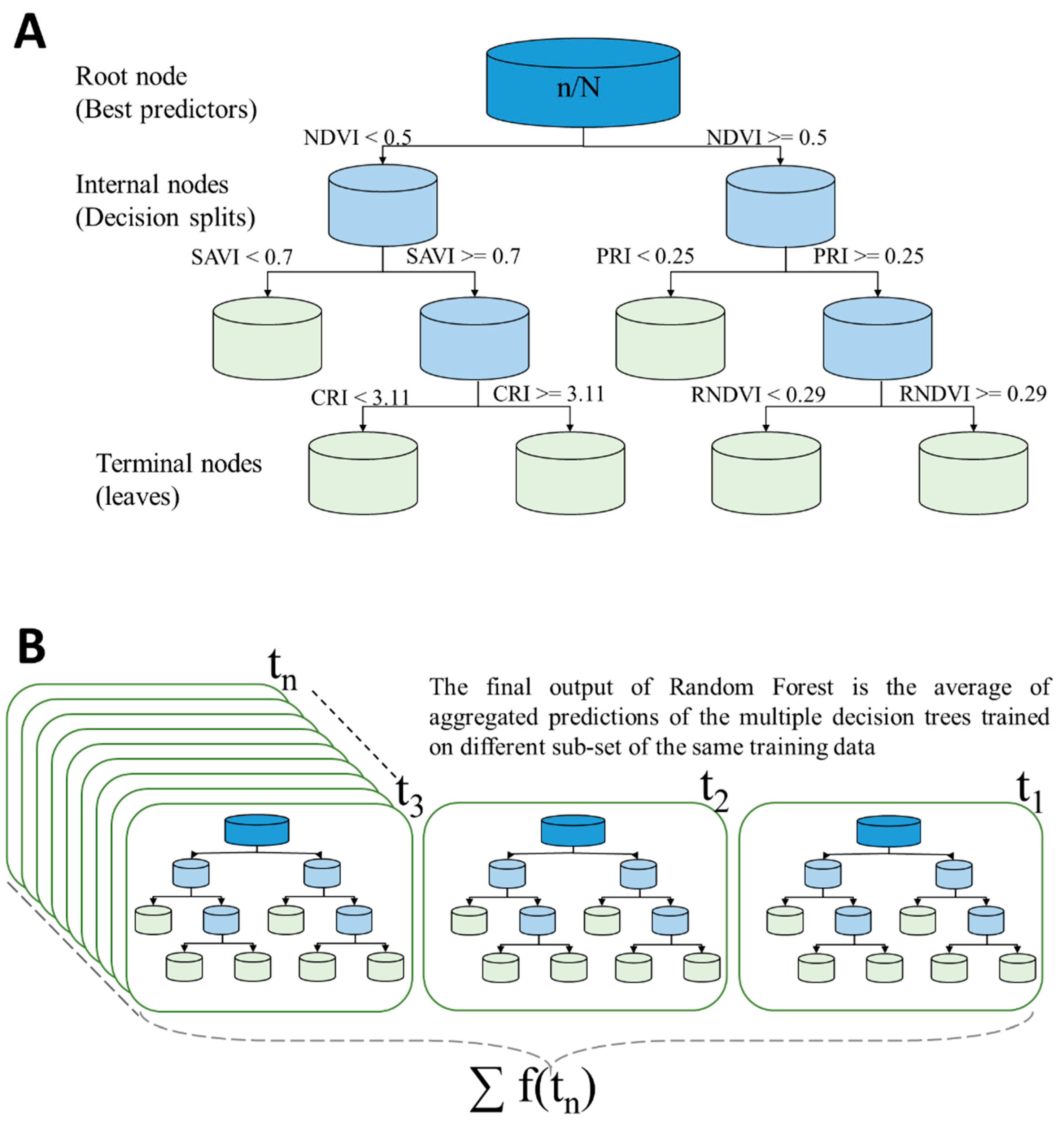
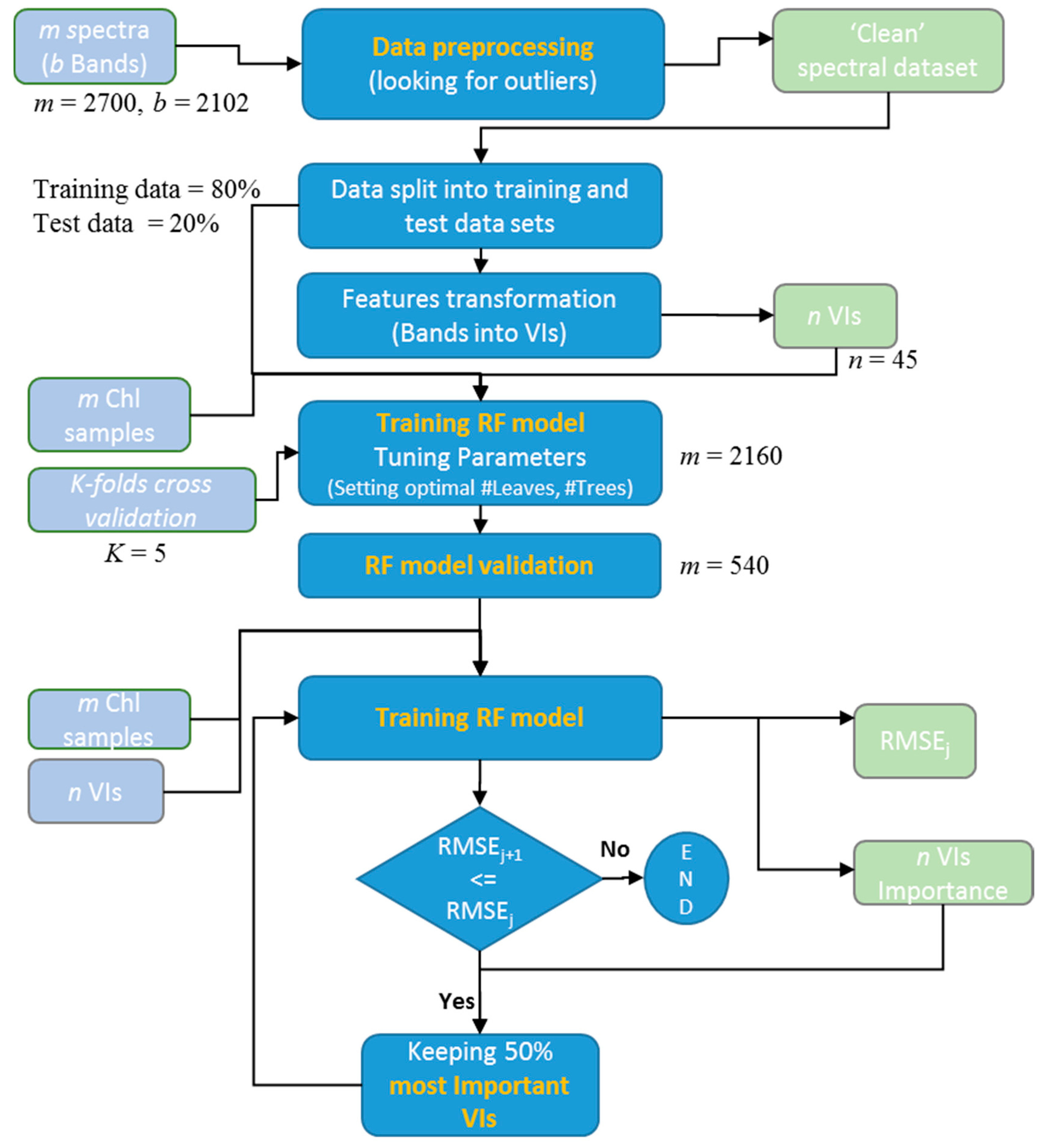
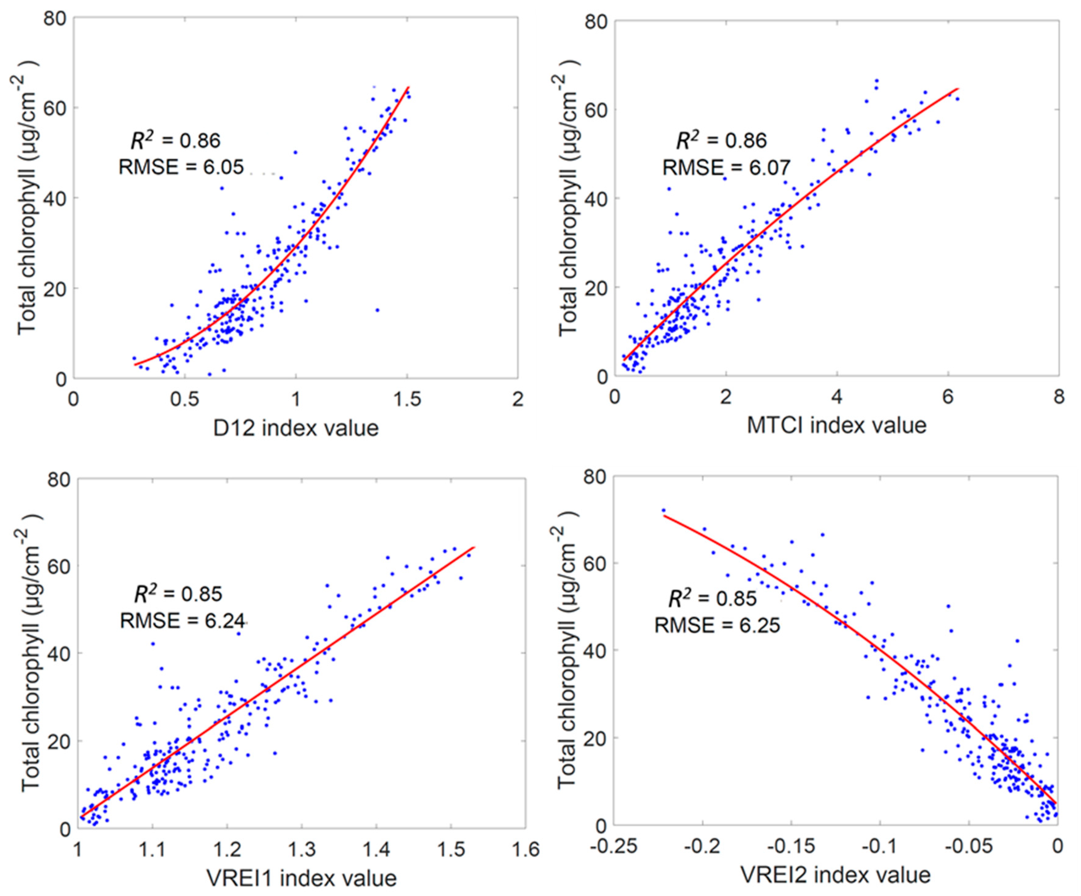
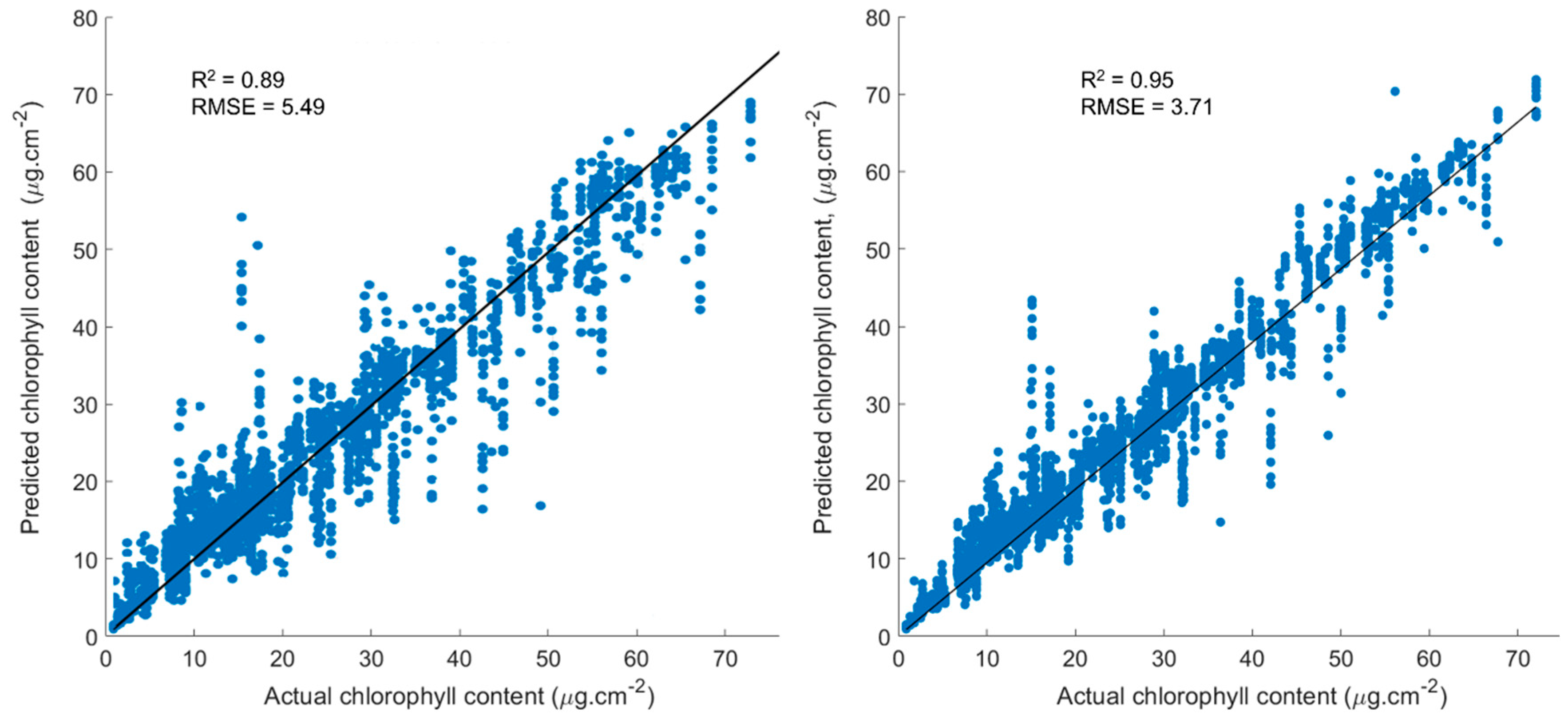
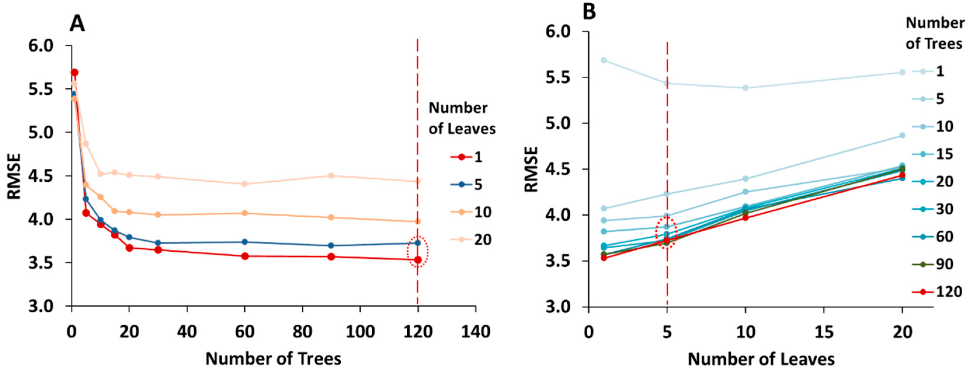
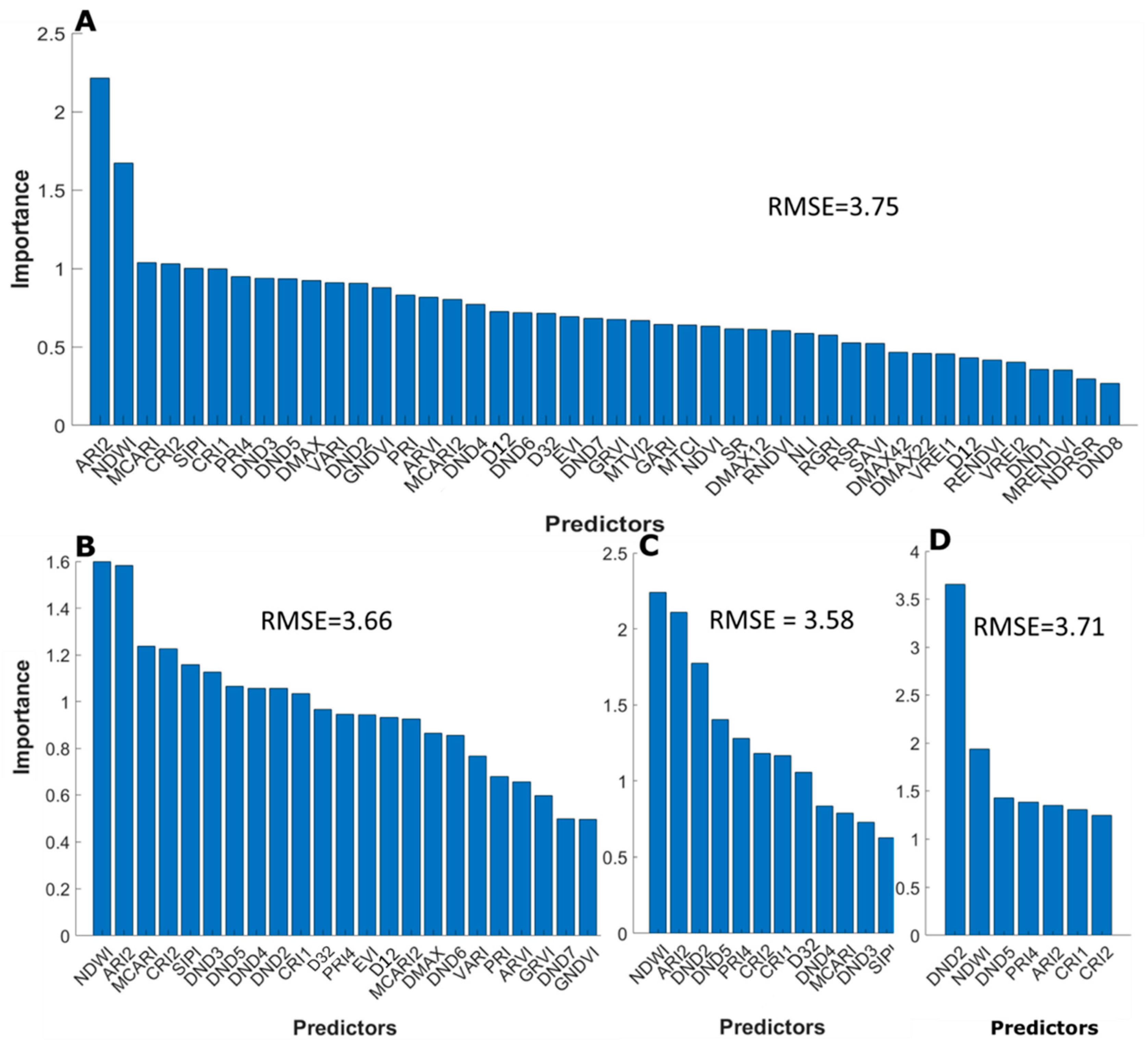
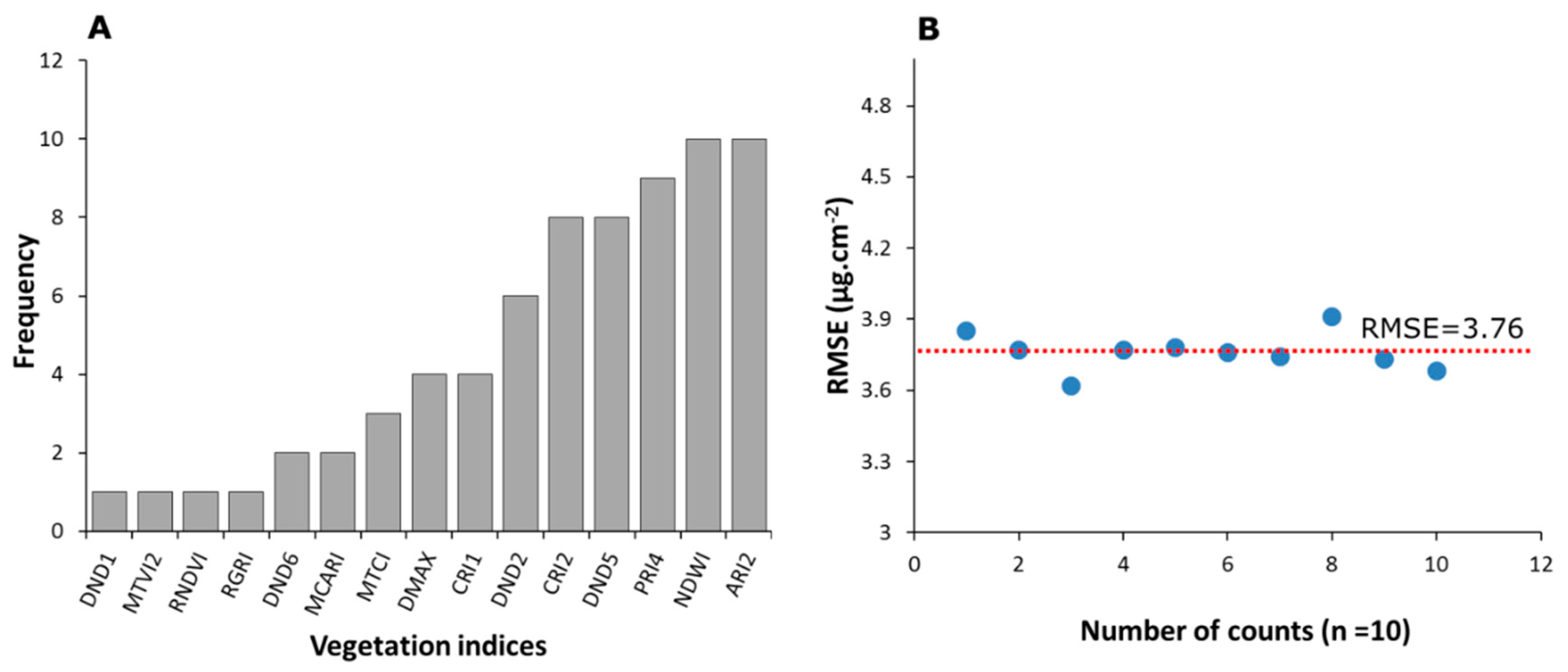
Table 1.
The 45 selected vegetation indices examined in this research, together with their band-specific formulations, predominant application, and associated principal reference.
Table 1.
The 45 selected vegetation indices examined in this research, together with their band-specific formulations, predominant application, and associated principal reference.
| No | Name | Vegetation Index | Application | |
|---|---|---|---|---|
| 1 | Anthocyanin Reflectance Index [40] | Carotenoids | ||
| 2 | Atmospherically Resistant Vegetation Index [41] | Vegetation | ||
| 3 | Carotenoid Reflectance Index 1 [42] | Carotenoids | ||
| 4 | Carotenoid Reflectance Index 2 [42] | Carotenoids | ||
| 5 | Enhanced Vegetation Index [43] | Vegetation | ||
| 6 | Green Atmospherically Resistant Index [44] | Chlorophyll | ||
| 7 | Green Norm. Difference Vegetation Index [45] | Chlorophyll | ||
| 8 | Green Ratio Vegetation Index [46] | Pigments | ||
| 9 | Modified Chlorophyll Absorption Ratio Index [47] | Chlorophyll | ||
| 10 | Modified Chlorophyll Absorption Ratio Index Improved [48] | Vegetation | ||
| 11 | Plant Senescence Reflectance Index [49] | Pigments | ||
| 12 | MERIS Terrestrial Chlorophyll Index [50] | Chlorophyll | ||
| 13 | MERIS Terrestrial Chlorophyll Index 2 [51] | Chlorophyll | ||
| 14 | Modified Triangular Vegetation Index Improved [48] | Vegetation | ||
| 15 | Normalized Difference Red-edge Simple Ratio [52] | Chlorophyll | ||
| 16 | Normalized Difference Vegetation Index [53] | Vegetation | ||
| 17 | Normalized Difference Water Index [54] | Leaf water | ||
| 18 | Non-Linear Index [55] | Vegetation | ||
| 19 | Photochemical Reflectance Index [56] | Pigments | ||
| 20 | Photochemical Reflectance Index Improved [57] | Pigments | ||
| 21 | Red Edge Normalized Vegetation Index [49] | Chlorophyll | ||
| 22 | Red Green Ratio Index [58] | Pigments | ||
| 23 | Renormalized Difference Vegetation Index [59] | Chlorophyll | ||
| 24 | Red-edge Simple Ratio [52] | Chlorophyll | ||
| 25 | Soil Adjusted Vegetation Index [43] | Vegetation | ||
| 26 | Structure Insensitive Pigment Index [11] | Pigments | ||
| 27 | Simple Ratio Index [60] | Vegetation | ||
| 28 | Visible Atmospherically Resistant Index [42] | Vegetation | ||
| 29 | Vogelmann Red Edge Index [61] | Chlorophyll | ||
| 30 | Vogelmann Red Edge Index Improved [61] | Chlorophyll | ||
| 31 | Derivative Simple Ratio 02 | Vegetation | ||
| 32 | Derivative Simple Ratio 32 | Vegetation | ||
| 33 | Derivative Simple Ratio 12 | Vegetation | ||
| 34 | -----NDVIs based on the first derivatives (DND) over 650–750 nm domain----- | Maximum Derivative Index | Vegetation | |
| 35 | DMAX Simple Ratio with D712 | Vegetation | ||
| 36 | DMAX Simple Ratio D722 | Vegetation | ||
| 37 | DMAX Simple Ratio D742 | Vegetation | ||
| 38 | Normalized Difference Derivative 1 | Vegetation | ||
| 39 | Normalized Difference Derivative 2 | Vegetation | ||
| 40 | Normalized Difference Derivative 3 | Vegetation | ||
| 41 | Normalized Difference Derivative 4 | Vegetation | ||
| 42 | Normalized Difference Derivative 5 | Vegetation | ||
| 43 | Normalized Difference Derivative 6 | Vegetation | ||
| 44 | Normalized Difference Derivative 7 | Vegetation | ||
| 45 | Normalized Difference Derivative 8 | Vegetation | ||
Note: Normalized difference indices of the first derivative transformed narrow-bands (DND) were determined at various reflectance band combinations. First derivative Dλ was calculated as (Dλ+10 − Dλ−10)/20, where λ represents the reflectance band.
Table 2.
Regression analysis and curve fitting results of the selected vegetation indices versus chlorophyll content, ranked in descending order of goodness of fit (followed by ascending RMSE). Indices reported as being indicators of chlorophyll content (see Table 1) are highlighted in green.
Table 2.
Regression analysis and curve fitting results of the selected vegetation indices versus chlorophyll content, ranked in descending order of goodness of fit (followed by ascending RMSE). Indices reported as being indicators of chlorophyll content (see Table 1) are highlighted in green.
| No. | Vegetation Index | R2 | RMSE (µg cm−2) | No. | Vegetation Index | R2 | RMSE (µg cm−2) |
|---|---|---|---|---|---|---|---|
| 1 | D12 | 0.86 | 6.05 | 24 | DND3 | 0.43 | 12.41 |
| 2 | MTCI | 0.86 | 6.07 | 25 | SR | 0.39 | 12.74 |
| 3 | VREI1 | 0.85 | 6.24 | 26 | NDVI | 0.37 | 12.98 |
| 4 | VREI2 | 0.85 | 6.25 | 27 | DND4 | 0.35 | 13.22 |
| 5 | D02 | 0.85 | 6.26 | 28 | PSRI | 0.32 | 13.46 |
| 6 | MRENDVI | 0.85 | 6.34 | 29 | MCARI | 0.30 | 13.73 |
| 7 | DND1 | 0.85 | 6.36 | 30 | CRI1 | 0.27 | 13.96 |
| 8 | RSR | 0.85 | 6.38 | 31 | NLI | 0.26 | 14.03 |
| 9 | NDRSR | 0.85 | 6.39 | 32 | EVI | 0.24 | 14.22 |
| 10 | DND8 | 0.85 | 6.45 | 33 | ARI2 | 0.24 | 14.23 |
| 11 | DMAX22 | 0.85 | 6.47 | 34 | RNDVI | 0.24 | 14.25 |
| 12 | D32 | 0.83 | 6.71 | 35 | SAVI | 0.24 | 14.25 |
| 13 | DMAX42 | 0.82 | 6.91 | 36 | PRI4 | 0.24 | 14.30 |
| 14 | RENDVI | 0.82 | 6.97 | 37 | CRI2 | 0.22 | 14.49 |
| 15 | DND2 | 0.82 | 7.01 | 38 | MCARI2 | 0.20 | 14.63 |
| 16 | GRVI | 0.80 | 7.40 | 39 | MTVI | 0.20 | 14.63 |
| 17 | GNDVI | 0.79 | 7.42 | 40 | VARI | 0.17 | 14.88 |
| 18 | GARI | 0.79 | 7.55 | 41 | RGRI | 0.14 | 15.16 |
| 19 | DND7 | 0.78 | 7.64 | 42 | DMAX | 0.09 | 15.61 |
| 20 | DMAX12 | 0.62 | 10.09 | 43 | NDWI | 0.08 | 15.66 |
| 21 | PRI | 0.54 | 11.12 | 44 | DND5 | 0.02 | 16.21 |
| 22 | SIPI | 0.53 | 11.27 | 45 | DND6 | 0.01 | 16.30 |
| 23 | ARVI | 0.43 | 12.32 |
© 2019 by the authors. Licensee MDPI, Basel, Switzerland. This article is an open access article distributed under the terms and conditions of the Creative Commons Attribution (CC BY) license (http://creativecommons.org/licenses/by/4.0/).
Share and Cite
MDPI and ACS Style
Shah, S.H.; Angel, Y.; Houborg, R.; Ali, S.; McCabe, M.F. A Random Forest Machine Learning Approach for the Retrieval of Leaf Chlorophyll Content in Wheat. Remote Sens. 2019, 11, 920. https://0-doi-org.brum.beds.ac.uk/10.3390/rs11080920
AMA Style
Shah SH, Angel Y, Houborg R, Ali S, McCabe MF. A Random Forest Machine Learning Approach for the Retrieval of Leaf Chlorophyll Content in Wheat. Remote Sensing. 2019; 11(8):920. https://0-doi-org.brum.beds.ac.uk/10.3390/rs11080920
Chicago/Turabian StyleShah, Syed Haleem, Yoseline Angel, Rasmus Houborg, Shawkat Ali, and Matthew F. McCabe. 2019. "A Random Forest Machine Learning Approach for the Retrieval of Leaf Chlorophyll Content in Wheat" Remote Sensing 11, no. 8: 920. https://0-doi-org.brum.beds.ac.uk/10.3390/rs11080920
Note that from the first issue of 2016, this journal uses article numbers instead of page numbers. See further details here.