Review

Sun-Induced Chlorophyll Fluorescence II: Review of Passive Measurement Setups, Protocols, and Their Application at the Leaf to Canopy Level

1
Crop Science Group, Institute of Agricultural Sciences, ETH Zurich, Universitätstrasse 2, 8092 Zurich, Switzerland
2
Laboratory for Earth Observation, Image Processing Laboratory, University of Valencia, C/ Catedrático José Beltrán, 2, 46980 Paterna, Spain
3
Finnish Meteorological Institute, Erik Palmenin Aukio 1, P.O. Box 501, 00101 Helsinki, Finland
4
Department of Geography, University of Zurich, Winterthurerstrasse 190, 8057 Zurich, Switzerland
5
Eawag, Swiss Federal Institute of Aquatic Science and Technology, Überlandstrasse 133, 8600 Dübendorf, Switzerland
6
Ecole polytechnique, Centre National de la Recherche Scientifique, Sorbonne Université, Ecole Normale Supérieure de Paris, Laboratoire de Météorologie Dynamique, LMD, F-91128 Paris, France
7
Centre of Excellence PLECO (Plants and Ecosystems), Department of Biology, University of Antwerp, 2000 Antwerp, Belgium
8
Geography and Spatial Sciences, School of Technology, Environments and Design, College of Sciences and Engineering, University of Tasmania, Private Bag 76, 7001 Hobart, Australia
9
Max Planck Institute for Biogeochemistry, Hans-Knöll-Straße 10, D-07745 Jena, Germany
10
Faculty of Science and Technology, Free University of Bozen/Bolzano. Universitätsplatz 1—piazza Università 1, 39100 Bozen-Bolzano, Italy
11
JB Hyperspectral Devices, 40225 Düsseldorf, Germany
12
Remote Sensing of Environmental Dynamics Lab., DISAT, University of Milano-Bicocca, Piazza della Scienza 1, 20126 Milano, Italy
13
Institute of Bio- and Geosciences (IBG-2): Plant Sciences, Forschungszentrum Jülich GmbH, Leo-Brandt-Str., 52428 Jülich, Germany
14
GeoSciences University of Edinburgh, King’s Buildings, West Mains Road, Edinburgh EH9 3FF, UK
*
Authors to whom correspondence should be addressed.
Submission received: 8 March 2019 / Revised: 10 April 2019 / Accepted: 11 April 2019 / Published: 16 April 2019

Abstract

:
Imaging and non-imaging spectroscopy employed in the field and from aircraft is frequently used to assess biochemical, structural, and functional plant traits, as well as their dynamics in an environmental matrix. With the increasing availability of high-resolution spectroradiometers, it has become feasible to measure fine spectral features, such as those needed to estimate sun-induced chlorophyll fluorescence (F), which is a signal related to the photosynthetic process of plants. The measurement of F requires highly accurate and precise radiance measurements in combination with very sophisticated measurement protocols. Additionally, because F has a highly dynamic nature (compared with other vegetation information derived from spectral data) and low signal intensity, several environmental, physiological, and experimental aspects have to be considered during signal acquisition and are key for its reliable interpretation. The European Cooperation in Science and Technology (COST) Action ES1309 OPTIMISE has produced three articles addressing the main challenges in the field of F measurements. In this paper, which is the second of three, we review approaches that are available to measure F from the leaf to the canopy scale using ground-based and airborne platforms. We put specific emphasis on instrumental aspects, measurement setups, protocols, quality checks, and data processing strategies. Furthermore, we review existing techniques that account for atmospheric influences on F retrieval, address spatial scaling effects, and assess quality checks and the metadata and ancillary data required to reliably interpret retrieved F signals.

Graphical Abstract

1. Introduction

Imaging and non-imaging spectroscopy enables the detailed assessment of biochemical, structural, and even functional attributes of vegetation in natural environments at multiple scales [1,2]. It has now been performed for more than 30 years [3,4]. During this period, the technologies for spectroradiometric measurements have greatly advanced. Today, many high spectral resolution spectroradiometers (often used synonymously with spectrometer, although the latter is radiometrically calibrated) are available, and they are operated from different measuring platforms: (1) ground-based at the leaf level [5,6,7]; (2) ground-based at the canopy level, either carried by people or mounted on towers and other platforms [8,9,10,11]; (3) airborne-based at the canopy level, flown at low-altitudes on, for example, UAVs [12,13,14,15,16,17,18]; (4) at high altitudes by aircraft [19,20,21]; and (5) spaceborne-based [22,23,24,25]. This diversity provides the opportunity to monitor the dynamics of vegetation on different spatial and temporal scales. With advancements in sensor technology, these instruments can also measure fine spectral features. An example is sun-induced chlorophyll fluorescence (F), which is retrieved by exploiting telluric oxygen absorption bands (i.e., at 685 nm and 760 nm) [19] and single Fraunhofer lines [26,27].
F emitted by chlorophyll-a molecules is one of three main de-excitation mechanisms for the energy captured by the light-harvesting pigments of plants. Under natural conditions, F represents only a few percent of the reflected radiance. Thus, detecting F is particularly challenging. Chlorophyll fluorescence has been widely used as a probe for photosynthesis at the level of chloroplasts, leaves, and plants in the laboratory and field studies (for reviews cf. [28,29]). In the vast majority of these studies, an active light source was used to induce fluorescence, limiting the application of these active methods to setups in which close contact with the leaf is possible. However, there have been a few attempts to use these active approaches with a distance to the canopy of several meters [30,31,32,33].
The ability to detect F with passive instruments largely extended the distance range and opened new possibilities to monitor functional vegetation dynamics at the ecosystem, landscape, or even global scale. Measurement setups and protocols for ground-based optical measurements have been already homogenized, e.g., for European flux sites [34], within the international SpecNet consortium [35], and for phenology monitoring [36,37]. F measurement protocols, however, require particular consideration to prevent the misinterpretation of retrieved F signals due to its sensitive behavior in response to environmental factors and challenges related to the retrieval of this small signal. Furthermore, the very dynamic nature of F compared with other common vegetation traits derived from spectral data (e.g., chlorophyll content, leaf area index) makes the measurement setup and post-processing even more challenging, and it requires the careful consideration of environmental, physiological, structural, instrumental, and experimental aspects during radiometric measurements and F retrievals (Figure 1). Additionally, measurements of F at different levels (e.g., leaf and canopy) and scales (single leaf to landscape) require different protocols and attempts to link such cross-scale measurements. This also includes considerations given to necessary meta- and ancillary data.
Meeting these challenges requires not only reliable measurement setups, sophisticated measurement protocols, and robust F retrieval methods but also properly calibrated and characterized instruments. For the past four years, many researchers have worked within the framework of the European Cooperation in Science and Technology (COST) Action ES1309 to meet the aforementioned challenges by developing innovative optical tools for proximal sensing of ecophysiological processes (OPTIMISE; https://optimise.dcs.aber.ac.uk/). The OPTIMISE community has compiled three papers on instrument characterization [38], measurement setups and protocols (this paper), and retrieval techniques [39] to make the gathered information available to the community. The set of papers aims to summarize the state-of-the-art for highly precise radiance measurements with a focus on F to complement other review papers on the emerging topic of F spectroscopy ([40,41], Mohammed et al., in press). The aim of this paper is to provide an overview of the subject and discuss proximal and airborne measurement setups and protocols currently used to retrieve F from spectrally resolved surface radiance (L) and incoming downwelling radiance (E) measurements. We differentiate between the leaf and canopy level.
After this introduction (Section 1), we first provide some brief background information on passive F measurements (Section 2) before reviewing ground and airborne measurement setups and protocols for F measurements on the leaf and canopy level (Section 3). Then, we review current approaches to address open challenges regarding atmospheric influences, quality checks, spatial scaling effects, and metadata and ancillary data (Section 4). In the end, we discuss the current approaches and offer an outlook.

2. Background

Plants use two photosystems (photosystem I and II, or PSI and PSII), which act in series to carry electrons from water to the final acceptor (NADPH) in the light-dependent reactions of photosynthesis and produce the energy-rich ATP molecule. At the PSI and PSII level, light is absorbed by various photosynthetic pigments (chlorophyll-a, chlorophyll-b, carotenoids), which results in excited states of chlorophyll-a molecules. This energy is then used by photochemical conversion to drive photosynthesis, while a small fraction of the excitation energy is re-emitted back as fluorescence. Under high light and stress conditions, excessive energy can dissipate in a controlled manner via various pathways that are classified as non-photochemical quenching mechanisms (NPQs). Because these three processes all dissipate the excitation energy, they are tightly interrelated. Hence, F can be quenched by photochemistry or NPQ dissipation, the latter being partially under the control of photoprotective mechanisms that help to safely dissipate excess energy [42].
Leaf F is emitted in the red and far-red range (from about 650 nm to 850 nm), with two peaks near 685 nm and 740 nm [43]. PSI and PSII have different antenna compositions and therefore different spectroscopic properties. PSI fluorescence is found to be emitted only in the far-red and stays almost constant, while PSII has two emission peaks in the red and far-red. PSII also exhibits variable fluorescence, mainly in response to the closure of reaction centers following a charge separation (photochemical quenching) and to increased heat dissipation (non-photochemical quenching).
Physiologically induced changes in F can be assessed by monitoring the fluorescence quantum yield (FY), defined as the ratio between fluorescence emission and the absorbed light evaluated on the basis of quanta fluxes. Alternatively, the fluorescence efficiency of a given surface can be estimated by the apparent spectral fluorescence yield (ASFY) as the ratio between the spectral fluorescence radiance in quanta units integrated over the emission hemisphere (e.g., in moles of photons m−2 s−1 nm−1 or W m−2 nm−1) to the incident light in the photosynthetic active radiation (PAR) region (e.g., in moles of photons m−2 s−1 or W m−2). At the leaf level, the ASFY is around 20 × 10−6 to 80 × 10−6 nm−1 [44], which gives a total apparent yield of about 0.2–0.8%. At the canopy level, different investigations have revealed values of the same order in the far-red (up to 30 × 10−6 nm−1) with generally lower values in the red (up to 8 × 10⁻⁶ nm−1) [45,46]. The level of the F signal can also be assessed by the fraction of fluorescence in the total vegetation radiance (emitted and reflected) at the same wavelength under natural sunlight. Outside the absorption bands, these fractions are found to be around 1% in the far-red and 10% in the red, the latter value being due to vegetation’s strong absorption in the red [47].
In order to detect weak F signals, telluric and solar (so-called Fraunhofer lines) atmospheric absorption features are generally exploited. Because fluorescence adds to the reflected surface radiance, it induces a subtle but detectable change in the spectral signature of the absorption lines. Over the many absorption lines that overlap the F emission, the ones in the O2-A and O2-B with a maximum absorption at 760 and 687 nm are particularly suitable for F detection, as they include a large number of close lines and correspond to the two F peaks.
As described in [40], retrieval methods that are used to quantify F are subdivided into two major categories: reflectance-based and radiance-based approaches. Radiance-based approaches are the most frequently used for the proximal sensing of F and include the Fraunhofer line discriminator (FLD) approach using two spectral bands [48,49], FLD approaches based on three or four bands (i.e., 3FLD, 4FLD) [11,50]), the improved FLD (iFLD) method [51], and the spectral fitting method (SFM) [52,53]. A common aspect among all of these methods is that measurements of E and L inside and outside the atmospheric absorption band are combined to decouple F from L. The decoupling relies on assumptions of F and reflectance (R) inside the exploited absorption feature, while the assumptions applied to estimate F and R inside the absorption band basically allow for categorizing using retrieval approaches. The FLD and 3FLD methods require 1 and 2 spectral measurements outside the absorption bands to estimate F and R inside the band. The iFLD approach uses a polynomial fit and some correction factors to estimate F and R inside the band using several spectral bands that are outside. The SFM method uses the full spectrum’s information around the absorption band to decouple F and L by spectral curve fitting. The method relies on general mathematical functions that represent canopy R and F around and within spectral windows centered at oxygen absorption bands (for further discussion on the retrieval methods, see [39] (in review, this issue)).
In vivo passive fluorescence detection from remote sensing measurements was initiated in the 1980s [54] and further developed in the 1990s. It has made significant progress since then, with currently more than 50 papers per year on the subject (according to the Web of Science database). Reliable F retrievals rely on precise and spectrally detailed L measurements in very narrow parts of the spectrum, while the F signal is small. This requires very accurate measurements (spectrally and radiometrically) of L (and E) and, in consequence, necessitates a common approach/protocol to be established for such measurements to enable reliable and consistent F retrievals.

3. Measuring F on the Leaf and Canopy Level

3.1. Leaf Level

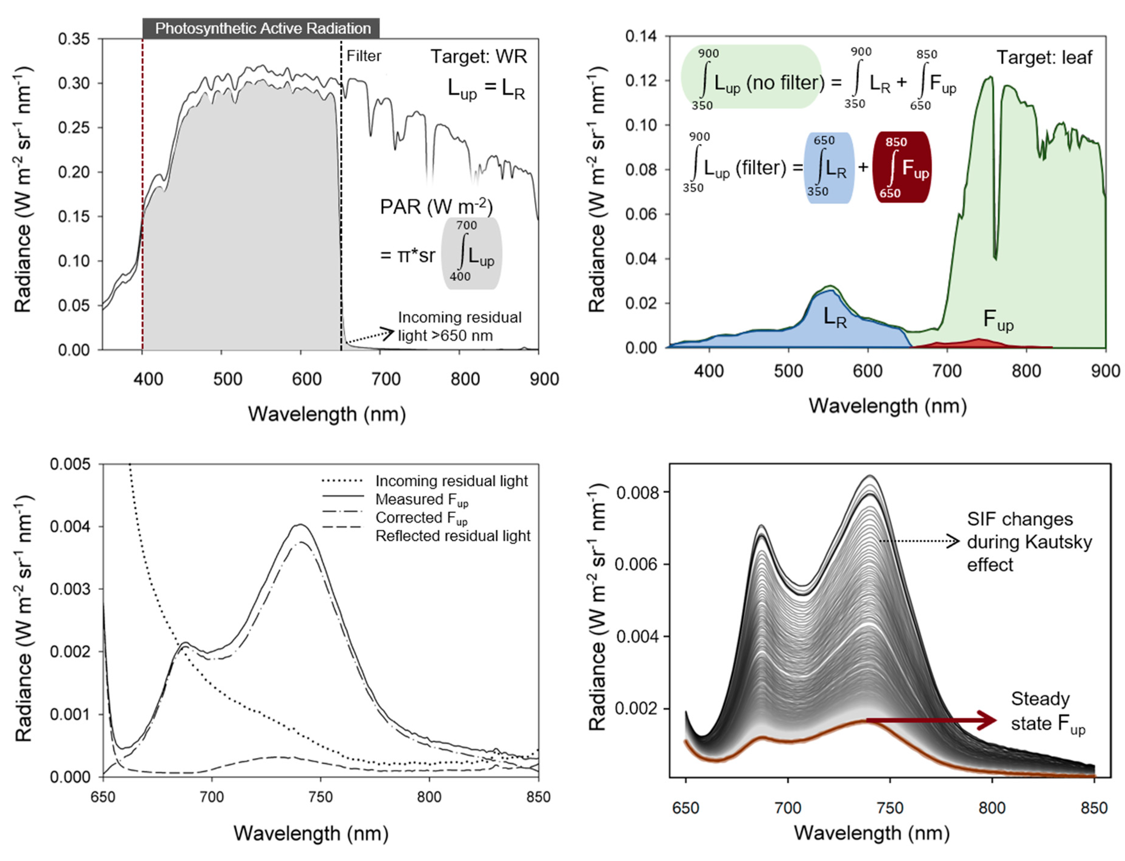
3.1.1. Measurement Setups

The full range of emitted leaf fluorescence (600–800 nm) was originally measured in the laboratory with visible (VIS) near-infrared (NIR) spectrometers and detectors (e.g., 1024-channel intensified diode array detectors) using single-wavelength light sources, such as lasers, to prevent interference with the F emission range [5,31,55]. However, single-wavelength excitation sources have the disadvantages that (1) they impact the spectral shape as a result of the wavelength-specific absorbance and emission [56] and therefore affect the apparent spectral fluorescence yield (ASFY) emitted by the leaf; (2) the applied illumination often represents only a fraction of the natural illumination conditions, and the plant reacts differently depending on the light intensity; and (3) they do not allow the simultaneous retrieval of ancillary data from the reflectance signal (e.g., Chl content, Photochemical Reflectance Index (PRI)) in the PAR (W m−2) range. Therefore, the use of a natural(-like) illumination source (lamp or sun) that provides a realistic PAR range is commonly preferred in the case of remote sensing applications, whereby the (full-range, spectrally resolved) F signal is measured in physical radiance units by a spectroradiometer. Measuring under natural(-like) light conditions, however, requires a retrieval method to decouple F from L. Using any of the remote sensing methods would also be possible at the leaf level, but the setup could be difficult, susceptible to the uncertainties associated with those indirect methods and limited to certain wavelengths. A more direct and practical approach is the use of a band-pass filter (see setups by [57,58,59,60]) to omit the incoming light that interferes with the F range (i.e., >650 nm) and only slightly overlaps with the PAR range. For practical convenience, the FluoWat leaf clip was developed [61], which uses a filter that is easily inserted and removed and enables the insertion of a fiber optic in both the top and bottom positions to measure the upward and downward radiance fluxes perpendicular to the leaf surface (Lup(λ), Ldw(λ), W m−2 sr−1 nm−1, Figure 2). The placement of a sharp-edge low-pass filter (e.g., a high-performance OD4 short-pass filter, TechSpec, Edmund Optics GmbH, Germany) cuts off wavelengths longer than 650 nm, and upward and downward leaf-emitted F fluxes (Fup(λ), Fdw(λ), W m−2 sr−1 nm−1) can be directly measured in the full 650–850 nm range [62]. The instrument requirements for measuring F directly under a low-pass filter are less strict compared with those for F retrieval from the narrow O2-absorption features (e.g., full-width at half maximum (FWHM) < 1 nm, SSI < 1 nm, see Section 3.2, Supplementary Table S2). Spectrometers used in combination with a filter to omit light that interferes with F should nevertheless comprise a sufficiently high signal-to-noise ratio (SNR) because the radiative flux is relatively weak (approx. 2.5 mW m−2 sr−1 @740 nm) (Supplementary Table S2); an example of this type of spectrometer is the FieldSpec (Analytical Spectral Devices (ASD) Inc., Boulder, CO, USA) [6,63,64]. To better interpret the link between passively measured F and photosynthesis, many of these setups also combine an active pulse-amplified modulating (PAM) fluorometer [57,58,59], gas exchange system [65], and/or leaf thermocouple to derive in parallel the parameters that are directly linked to photochemical yield, CO2 uptake, and sensible heat dissipation.

3.1.2. Measurement Protocols

Leaf upward and downward radiance (Lup(λ) and Ldw(λ)) are respectively composed of the reflected and transmitted radiance (LR(λ), LT(λ), W m−2 sr−1 nm−1) measured in the VIS–NIR–short-wave infrared (SWIR) (depending on the spectrometer) and the upward and downward F emission (Fup(λ) and Fdw(λ), W m−2 sr−1 nm−1) in the red and far-red region (Figure 2). To decouple these radiance fluxes, leaf measurements are ideally taken as serial acquisitions of Lup and Ldw from an upward- and downward-pointing perspective perpendicular to the target surface, with and without a low band-pass filter (Figure 2). As an example, with the FluoWat leaf clip, a band-pass filter can be placed in front of the illumination opening, and LR and LT are omitted beyond 650 nm (Figure 3). Either a leaf or white reference (WR) target is inserted inside the clip while the clip is pointed toward a natural(-like) illumination source so that the light enters the light opening perpendicularly and forms an inclination angle of 45° with the leaf surface inside the chamber, creating a fixed sun-target-sensor geometry. In this way, the incoming illumination is less dependent on the solar elevation angle. When measuring under solar illumination, this perpendicular positioning can be verified by a small light beam hitting the center of the cross-hairs on both sides of the leaf clip. Because of the small light opening (1 cm diameter), a slight deviation from the angle of the sun inclination can induce shadowing on the leaf sample.
It is highly advisable to measure E or PAR before and after each series of leaf measurements in order to control the stability of the incoming illumination. Note that the white reference is a thin material and allows partial transmission; thus, a correction factor as a function of the wavelength for the WR material (due to wavelength-dependent reflectances across the full range) might be established by a single measurement of the WR transmitted irradiance. These actions increase the number of spectral measurements but are required for higher accuracy and a robust data quality check. To check whether the WR measurement is reasonable for the leaf measurements, the calculated leaf absorptance should be less than 1 at any spectral band over the full spectrum when no filter is used. The highly scattering far-red region (700–800 nm) is useful for checking this requirement. However, this will only enable the detection of underrepresented values of E, resulting in overestimated absorbance. An example of measuring protocol is presented, with the different measuring options shown. Additionally, instrumental settings (integration time and dark current correction) should be optimized and performed in real time for the incoming radiance arriving at the target (WR or leaf) during the measurements to obtain the highest dynamic range and SNR possible.
The F signal, however, needs further processing. If the used band-pass filter does not cut off the light sharply at 650 nm (to be verified with a WR target measurement), some residual light may pass through the filter and add to the Fup signal as reflected residual light, calculated as the residual light passing the filter times the calculated leaf reflectance. After removal of this reflected residual light, the Fup is added to the Fdw signal, giving the total F leaving the leaf’s surface (Figure 3).
Overall, it should be kept in mind that F is driven in the first order by E, and that further changes are driven by the functional state of the leaf, thus altering the fluorescence yield (FY) [67,68]. Hence, because photoprotection mechanisms are activated, the relationship between FY and photosynthetic yield will differ between the morning and the afternoon (i.e., at similar irradiance conditions). This hysteresis effect should be kept in mind when designing protocols for measuring F in the field at a certain moment of the day. It further implies that additional ancillary data (cf. Section 4.3) are required for the correct interpretation and relation between F and photosynthesis.

3.2. Canopy Level

When measuring F at the canopy level, it is not possible to block sunlight in the manner discussed previously with the low-pass filter of a leaf clip. Thus, F can only be estimated by decoupling the emitted and reflected radiance of the canopy. This is challenging because of reabsorption effects, scattering within the canopy, and changing illumination under environmental conditions. While the first two processes are driven by the canopy radiative transfer, the latter can be compensated by the experimental setup used to measure F.

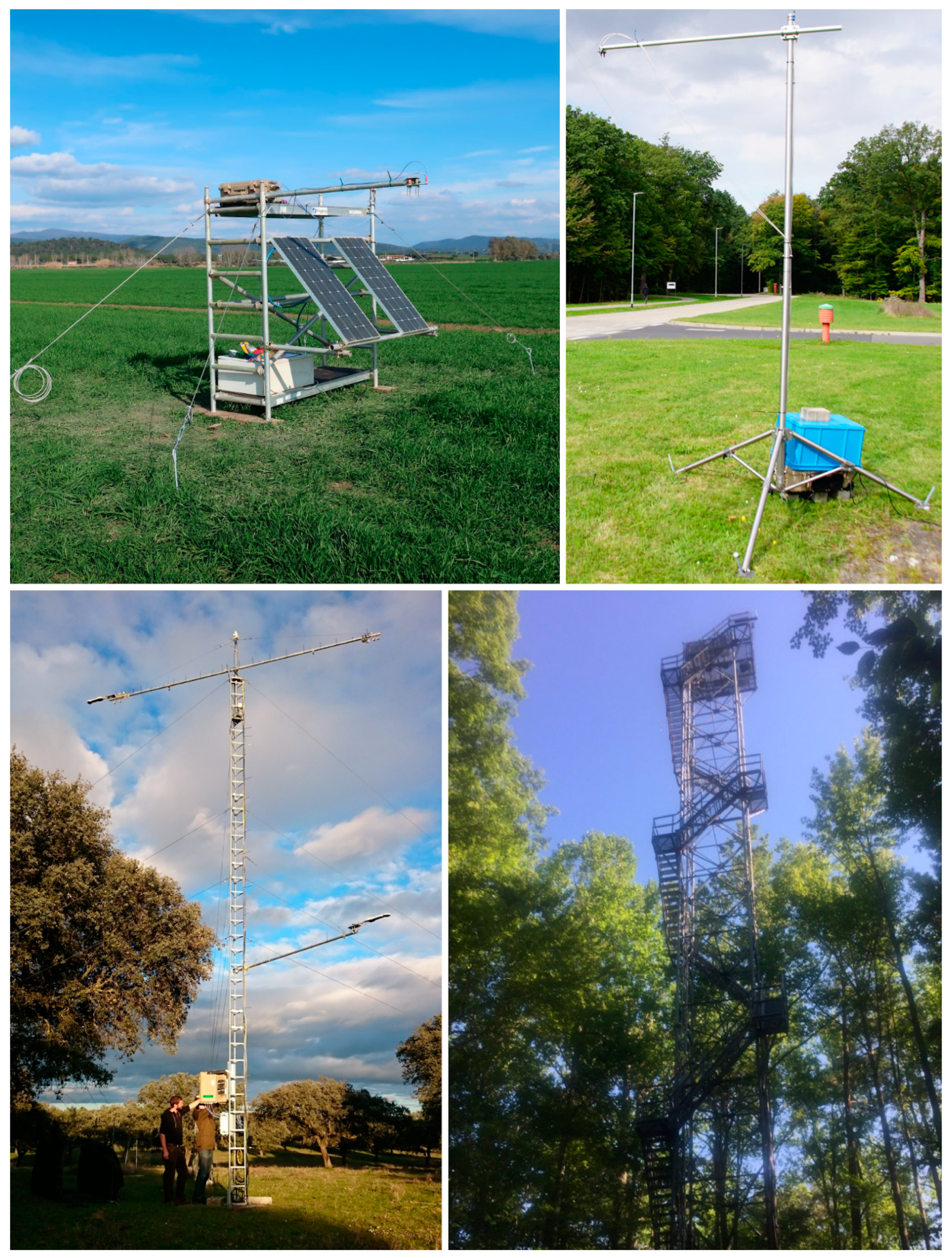
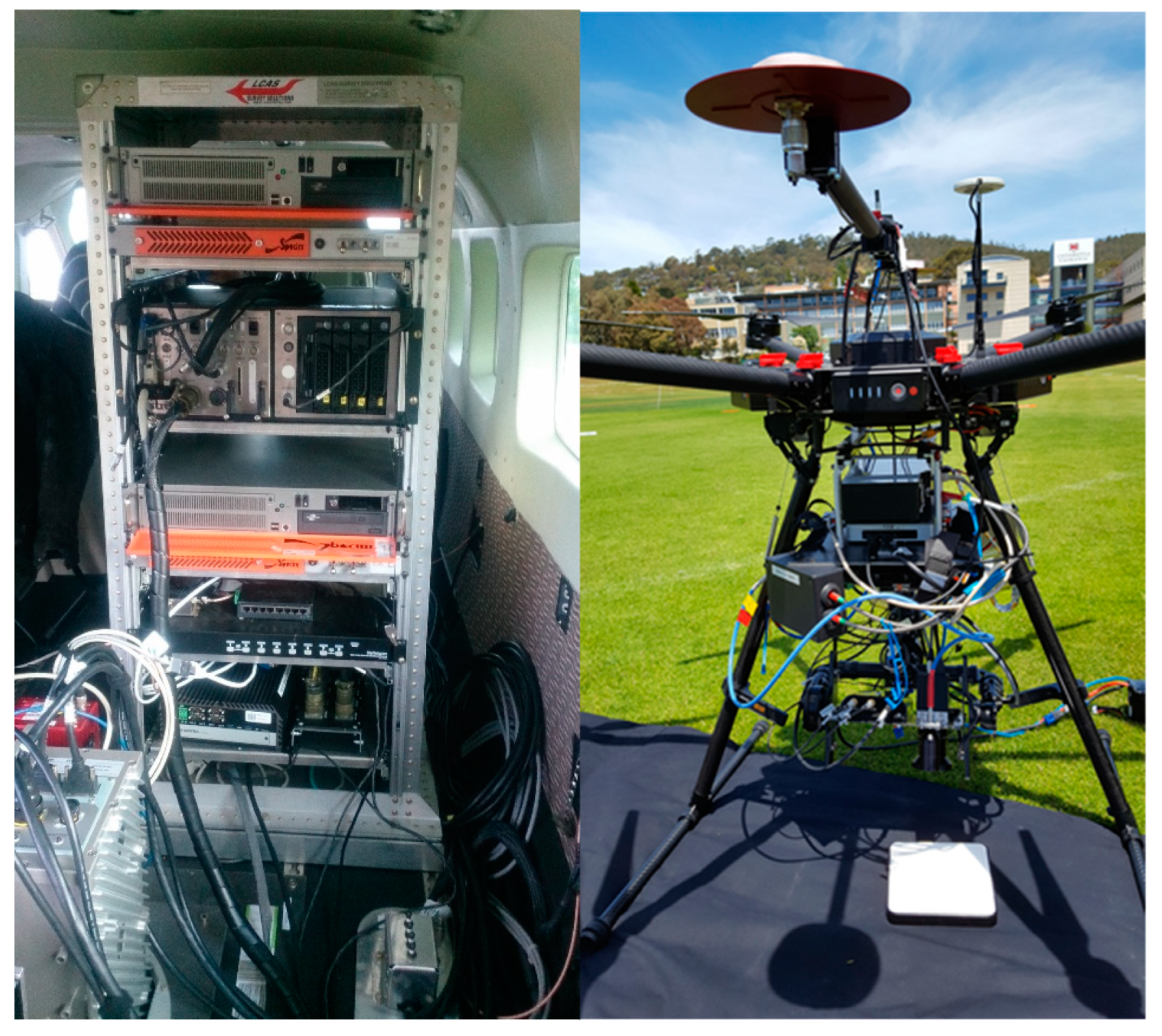
3.2.1. Measurement Setups from Proximal to the Airborne Scale

A variety of spectroradiometers with different fore-optics and control systems are used to retrieve F. While some of the spectroradiometers already mentioned in the review in [40] are still used to measure F, overall, the trend has been toward spectroradiometers with higher spectral resolution. Today, the most used are spectroradiometers with different configurations from Ocean Optics, Inc. (Dunedin, FL, USA) [69]: HR2000+ [8,11,46,47,70], HR4000 [10,71,72,73,74], QE Pro [17,74,75,76], and USB4000 [14,77] (Supplementary Table S2).
Ground-based setups that monitor the vegetation fluorescence emission employ several types of instruments that range from 10−1 to 101 m above the canopy (Figure 4). Such permanently installed and automated systems can be used to follow the diurnal and seasonal changes in F. One example is the FloX (JB Hyperspectral Devices UG, Düsseldorf, Germany), which is specifically designed to passively measure F under natural light conditions and is equipped with the QE Pro spectroradiometer. The instrument is based on prototypes, such as the Multiplexer Radiometer Irradiometer (MRI) [10], SFLUOR box, and SIF-System [78], developed by a collaboration between the Research Center Jülich and the Remote Sensing of Environmental Dynamics Laboratory of the University Milano Bicocca. At the time of writing this manuscript, about 20 FloX instruments have been deployed worldwide. A similar system is the FluoSpex 2. It also consists of two spectroradiometers—a QE Pro and an HR2000+. A network of such systems called FluoNet has been deployed for various ecosystems, including grassland, forests, and agricultural fields [79]. Another spectroradiometer system (Piccolo) was developed by a group at the University of Edinburgh [17]. This system can also incorporate up to two Ocean Optics spectroradiometers that cover different spectral regions and has a custom-designed double-bifurcated fiber optic assembly. This approach enables the almost simultaneous measurement of L and E by each spectroradiometer. In addition, the Piccolo fiber optic assembly incorporates fore-optics with integral shutters so that there is no light loss at in-line shutter interfaces. There are currently 10 Piccolo systems in use either at fixed installations or mounted on tractors or rotary-wing UAVs.
Often, the systems are mounted several meters above the canopy on or close to flux towers for purposes such as the evaluation of the relationship between F and parameters such as gross primary productivity (GPP) [8,75,76,77]. Specialized structures have been developed to measure F from greater heights. One example is the TriFLEX system [11]. It consists of a 21-meter-high crane equipped for F measurements. The crane is installed in the middle of fields dedicated to agricultural research. Owing to a 24-meter jib and a 100-meter railway, F measurements can be performed for nadir-viewing over a plot of 100 × 200 m and a plot of 60 × 150 m with field crops. Often, the spectroradiometers of fixed installation systems are shielded from the environment to stabilize their temperature [11,72]. This is necessary to keep the noise levels, the radiometric response, and especially the spectral features of the spectroradiometer constant [38] (in review, this issue). Additionally, the measurement of the downwelling E is a critical component. Ideally, it should be measured close to the target and exposed to a similar E field and not be shaded or illuminated by other targets. Depending on the setup, this is not always straightforward, especially when cosine diffusers requiring a fixation structure are used. When the downwelling E is measured using a calibrated highly reflective reference (usually a Spectralon® panel (Labsphere, Inc., North Sutton, NH, USA)), the challenge is to place it appropriately (fixed level and in a similar E field as the target). Any reference surface (WR panel, cosine diffuser) should be kept free from dirt due to birds, insects, or dust and periodically checked for degradation [80]. Furthermore, the fiber optics should be tightly fixed since any movement will alter the radiometric throughput, leading to inappropriate calibration coefficients being applied. Several of the mentioned systems are used for calibration and validation efforts in the framework of the ESA FLEX mission preparation.
However, imaging spectroradiometers are also used. The SPECIM PS V10E (Specim, Spectral Imaging Ltd., Oulu, Finland) [81] is a pushbroom system with 1392 spatial pixels. The sensor was mounted on a long scanning bar, which was used to move the system and generate 2D hyperspectral images of the canopy. A custom-made retrieval with careful preprocessing facilitated the retrieval and spatial mapping of F from this ground-based imagery [9,82]. Recently, the high-performance ground-based imager HyScreen (Specim, Spectral Imaging Ltd, Oulu, Finland) has been developed particularly to derive F.
Canopy measurements are also carried out using airborne platforms. The first airborne instrument dedicated to measuring F was the AIRFLEX multichannel radiometer [83]. Less than 10 years after that, the HyPlant imaging spectroradiometer system ([19], Figure 5, left) was developed to serve as an airborne demonstrator for the European Space Agency’s Earth Explorer mission Fluorescence Explorer (FLEX) [84]. The sensor package operates in the pushbroom mode and consists of two optical imaging modules: (1) the DUAL-imager, a line-imaging VIS–NIR–SWIR spectroradiometer consisting of two sensors integrated in a single housing using common fore-optics to provide contiguous spectral information from 370 to 2500 nm, with a 3 nm spectral resolution in the VNIR spectral range and 10 nm spectral resolution in the SWIR spectral range; (2) the fluorescence imager (FLUO), a special module that acquires data at a very high spectral resolution (0.25 nm) in the spectral regions of the two atmospheric oxygen absorption bands (670–780 nm) and is dedicated to measuring F [19,73,85,86,87,88]. Other airborne sensors not specifically designed to retrieve F have also been used. Damm et al. [89] investigated the impact of varying irradiance on vegetation indices and F derived from spectroscopy data captured with the Airborne Prism Experiment (APEX) [20] and compared APEX-based F retrievals with EC-derived GPP. APEX is an airborne dispersive pushbroom imaging spectroradiometer covering the 375–2500 nm spectral region in up to 532 narrow contiguous spectral bands. The Chlorophyll Fluorescence Imaging Spectroradiometer (CFIS) [90,91] has also been used to retrieve F from aircraft.
F measurements have also been carried out from UAV platforms. These were predominantly carried out with fixed-wing platforms at ground altitudes of above 500 m and with instruments characterized by spectral resolutions of 5 nm and larger that were not specifically designed for F retrievals [16,92,93,94]. Very recently, multirotor UAV sensing systems were developed with a very high spectral resolution [14]. Another system that can also be carried on UAV systems is the Piccolo doppia [17]. Similar to the AirSIF system [95], illustrated in Figure 5 (right), it is based on the QE Pro spectroradiometer, and two fiber optics are used to measure the downwelling E and the L in a sequence. With the ongoing miniaturization of spectral sensing systems and the advances in robotics [12], we expect more UAV sensing systems to emerge in the future. Taking all systems together, the different observational scales could be interlinked and connected with the satellite observational scale [24,26,27,90]. Supplementary Table S2 gives an overview on different spectroradiometers, together with some example studies.

3.2.2. Measurement Protocols from Proximal to the Airborne Scale

Under natural outdoor conditions, the illumination changes constantly because the position of the sun changes throughout the diurnal and seasonal cycles and the composition of the atmosphere is highly dynamic. While cumulus clouds are rather visible changes, the unaided eye and human cognitive process might not perceive thin high-altitude cirrus clouds or changes in the aerosol or water content of the atmosphere [96]. Even changes in the air pressure influence the permeability of the atmosphere, and this influences the illumination at the top of the canopy, as well as affecting signal loss and scatter in the target-optics optical path. These changes are wavelength-dependent; they influence both the intensity of the irradiance and the irradiance field and affect the retrieval of biochemical plant parameters from spectral data and fluorescence [89].
Thus, for high-precision radiance measurements, such as the estimation of F, the measurement of the radiance emitted and reflected by the canopy and the irradiance received by it need to be captured nearly simultaneously to estimate a target’s spectral response to the illumination conditions present during the time of the acquisition [97]. The irradiance incident upon the target area can be approximated by measuring a diffuse (Lambertian) reflectance reference panel or by using a vertically pointing receptor that displays a cosine response. When only one spectroradiometer is used, this can be facilitated by alternating measurements of the reference and the target with the same fore-optic arrangement (single field-of-view (FOV) setup) or using a splitter and shutter system that switches between two fibers: one looking toward the target, and the other one looking toward a reference panel or a toward the zenith with an attached cosine receptor (dual FOV setup) [74,98]. The single FOV setup can be used manually or in an automated fashion with, for example, a rotation arm [99] or a moving panel [11,100]. Examples of the dual FOV setups are described in [8,73,76]. The setups can also be realized with multiple spectroradiometers, where one is typically pointed toward a reference target or an attached cosine receptor is pointed to the zenith, and the other one is pointed toward the vegetation target (dual spectroradiometer setup) [11,46,47]. There are also some special cases that turn their FOV toward the canopy and the zenith [99].
The dual spectroradiometer setup has the advantage that radiance and irradiance can be captured at nearly the same time. Unfortunately, two spectroradiometers never have the exact same spectral and radiometric characteristics. Thus, accurate cross-calibration is required and is very challenging; it is not always possible for very high spectral resolution spectroradiometers and likely to create biases in the data [14,98,101,102]. The impact of spectral shifts increases with the spectral resolution of the sensor. Pacheco-Labrador et al. [38] showed that when F retrieval relies on measured downwelling irradiances (not simulated with atmospheric radiative transfer models (RTMs)), any spectral shifts will induce errors that will only be canceled out if they affect the measurement of both (up- and downwelling) fluxes equally. In practice, this can only be achieved if they are recorded by the same sensor. Thus, the dual spectroradiometer approach is not recommended for F retrieval since it is incredibly sensitive to even sub-nanometric spectral shifts between the measured up- and downwelling radiation fluxes.
The different setups also differ by the viewing geometry that is used to measure surface radiance. Most setups adopt a nadir surface-viewing orientation. Also, in most cases, a bare fiber without fore-optics is used to measure the radiance of the canopy if the measurements are carried out rather close to the canopy. However, setups that measure farther away from the canopy often use lenses that limit the FOV [11] to constrain the extent of the area sampled. Some setups also use oblique-viewing geometries [8] and rotate to capture multiple targets [103,104,105]. Different viewing geometries have been shown to have a great impact on reflectance measurements for a given sun incidence angle [13,106,107,108]. The impact on F760 measurements were initially investigated in [82]. The authors found that F760 varied as a function of the sun’s incidence angle and viewing incidence angle during the midday measurement. In general, F760 tended to increase with higher viewing angles, especially when the sun incidence angle was between 35° and 100° with respect to the leaf normal. This needs to be accounted for if measurements with different viewing geometries are to be compared.
The subtlety of the F signal requires a robust measurement protocol that, on one hand, reduces the temporal offset of the reference and the target measurement and, on the other hand, optimizes the SNR of the instrument for the current illumination condition. The latter includes the optimization of the integration time, as well as an estimation of the dark current at that integration time and the current sensor temperature.
Most studies on F have reported that reference measurements are carried out quite close to canopy measurements. Most of the time, they are carried out sequentially (for cases in which just one spectroradiometer is used) [8,71]. For dual spectroradiometer setups, it is even possible to carry out both measurements simultaneously [11]. To use the full dynamic range of the spectroradiometer, the measurement integration time should be adapted to the current illumination. This is done either manually or by means of an auto-integrating function that iteratively changes the integration time until the sensor signal is within a range of predefined digital numbers that do not exceed the spectroradiometers saturation value. This can be done by optimizing either the integration time to the target or the target and reference channel. After the integration time is set, the actual measurements can start. In a typical measurement sequence, the canopy measurement is “sandwiched” between reference measurements [10,109]. Additionally, as an alternative to modeling the dark noise [110,111], it can also be quantified for the specified integration time(s) within the cycle by closing the shutters.
The further the distance between the object and the sensor, the more complex the atmospheric correction becomes (cf., Section 4.1.). Additionally, estimation of the irradiance is more complex at the airborne scale. While a few studies have used radiometric ground reference panels for an empirical correction, others have employed physical-based corrections [16,93,112]—for instance, those based on atmospheric transfer models, such as MODTRAN [113] or the SMARTS [114]—to estimate incoming radiance and other essential atmospheric transfer functions. For more specific applications, such as fluorescence retrievals, semi-empirical corrections of only selective wavelength regions are possible [115]. Some current UAV systems able the recording of the downwelling irradiance directly on the UAV (cf., AirSIF system in Figure 5), while other correction schemes are designed, although residual atmospheric disturbances typically remain [14]. The following section reviews the current knowledge on the need for atmospheric influence.

4. Current Approaches to Open Challenges of F Estimations from Proximal to Airborne Scale

4.1. Atmospheric Influences

One of the major challenges in measuring F is accounting for atmospheric influences. Oxygen’s absorption band-depth and spectral shape are affected by, for instance, changes in the surface pressure and temperature conditions [116] and the atmospheric scattering effects produced in the presence of aerosol and molecules [26]. At a distance of a few meters between the target and sensor, the effects of oxygen absorption must always be compensated in the strong O2-A band [117]. For larger target–sensor distances (e.g., when measurements are taken from UAVs or airborne and satellite platforms), not only oxygen absorption but also aerosol scattering plays a key role in both visible and near-infrared measurements [26] and must be, therefore, properly corrected.
At the canopy level, in order to disentangle F from the reflected solar irradiance, it is necessary to measure (1) the downwelling incident solar irradiance ( E ¯ ) and (2) the upwelling radiance from the surface ( L ¯ ), i.e., the reflected solar irradiance plus the contribution of the emitted F. Hereafter, the overlined symbol refers to magnitudes at the canopy level (see Figure 6). At a larger scale, on systems mounted on towers (e.g., [118,119]), the downwelling and the upwelling radiances are acquired at distances determined by the altitude of the sensor above the canopy (Figure 6). Similarly, when using UAV platforms, both downwelling and upwelling radiant fluxes are also measured at a distance determined by the altitude of the platform above the canopy, as the irradiance sensor is often mounted on the UAV. Conversely, when moving toward higher vertical scales, such as when using airborne platforms, only the upwelling radiance from the canopy is typically measured. Consequently, the use of an atmospheric RTM is required to simulate and estimate the actual incident solar irradiance at the canopy level. The following subsections discuss how atmospheric effects disturb the acquired radiance in the oxygen regions (O2-B and O2-A) for different vertical scales. In addition, we provide a short review of the current techniques typically applied to compensate for atmospheric effects when aiming to estimate F using passive remote sensing techniques.

4.1.1. High-Altitude Sensing

When measuring fluorescence using passive remote sensing techniques in the oxygen absorption regions from high-altitude airborne platforms, it is mandatory to compensate for atmospheric aerosol scattering and molecular absorption [120]. From the canopy, only the upwelling radiance, which is attenuated by its passage through the atmosphere, is typically measured at these altitudes (Figure 6). Thus, in order to estimate both E ¯ and L ¯ at the canopy level, the use of an atmospheric RTM is usually required. Generally, in order to characterize the atmospheric state to perform the atmospheric correction process, measurements related to the aerosol and water vapor content, as well as measurements related to the air temperature and pressure conditions, are normally acquired at the surface level. Thus, regardless of the selected atmospheric RTM, the model is commonly parametrized by making use of the ancillary atmospheric measurements acquired simultaneously to the airborne acquisitions (e.g., [120,121]).
In a past field campaign experiment [117], the researchers applied an oxygen transmittance compensation strategy as part of the FLD retrieval technique. In their work, an additional spectral correction factor of the transmittance was introduced by using non-fluorescence targets as a reference to compensate for the uncertainties associated with processing data that were mainly derived from assumptions made during the atmospheric modeling process. However, the use of non-fluorescence targets as a reference for calibration can also make the estimated fluorescence prone to errors in certain scenarios. The rationale behind this is that certain spectral artifacts (e.g., stray light) distort the absorption shape and depend on radiance levels. Therefore, radiometric calibration errors will impact bare soils and vegetated targets differently. Thus, in some cases, it may be preferable to use bare soil pixels only as a quality indicator to check the validity and quality of the applied radiometric and atmospheric correction process instead of using this data to derive a compensation factor [58].
As an alternative to the oxygen transmittance compensation applied in [115], any classical atmospheric correction technique based on the inversion of an RTM (as typically applied to data acquired from satellite platforms) can also be applied to correct airborne data. This way, all of the atmospheric transfer functions that account for the atmospheric scattering (the so-called path radiance) and the atmospheric backward reflection (the so-called spherical albedo) are determined together with the atmospheric transmittance (see [122] for more information regarding the approximations generally assumed in the atmospheric inversion formulation to estimate F).
Many RTM approaches are now available, such as the MODerate resolution atmospheric TRANsmission MODTRAN [113], the 6S code [123], and the LibRadtran RTM [124]. In general, the number of input parameters that need to be tuned will strongly depend on the flexibility of the selected model, as well as the ancillary information acquired that characterizes the atmospheric state. For instance, the majority of RTMs allow for configuring at least the viewing and illumination geometry, the aerosol presence, and the water vapor content. However, some RTMs, such as MODTRAN, allow the user to define a particular temperature vertical profile or parametrize the aerosol presence by defining a set of optical properties, such as the Aerosol Optical Thickness (AOT), the Angstrom exponent, the scattering asymmetry, the Single Scattering Albedo (SSA), or the aerosol vertical distribution. As expected, the more detailed the parametrization of the atmosphere, the more accurate the estimation of the canopy-level upwelling and downwelling radiances, which are required inputs for the majority of fluorescence retrieval strategies, e.g., the FLD or SFM family of techniques.

4.1.2. Low-Altitude Sensing

Although UAVs typically fly at lower altitudes (30–500 m) than aircraft, atmospheric effects are still strong for this range of target–sensor distances and must be compensated for prior to estimating fluorescence using passive remote sensing techniques. Similarly to other airborne acquisitions, atmospheric effects on UAV-acquired data mainly depend on (1) the platform altitude and (2) the concurrent atmospheric conditions. However, even in those cases in which the UAV is flying at lower altitudes, e.g., 100 m, atmosphere effects affect fluorescence measurements. Figure 7 shows the difference between simulated acquired upwelling radiances at the sensor level (UAV at 100 m) and at the surface level for two Aerosol Optical Thickness (AOT) settings, i.e., 0.03 [-] and 0.15 [-].
Aerosols significantly affect shorter wavelengths; i.e., they have a stronger impact on the O2-B than the O2-A spectral region. This can be observed in Figure 7 where the values outside the oxygen absorption regions, especially in the left panel, differ from 0 mW/m2/sr/nm. As expected, when the aerosol content is higher (red solid line), this effect is more noticeable. On the contrary, inside the oxygen absorption band, the spectral behavior is mainly dominated by the upward surface to the sensor oxygen transmittance.
Hence, although atmospheric effects can be neglected for many applications at the UAV scale, this is not the case when measuring the subtle fluorescence signal using passive remote sensing techniques and exploiting oxygen absorption features. In this respect, the atmospheric compensation techniques typically applied at the airborne scale can be equally suitable for correcting UAV-acquired measurements.

4.1.3. Ground-Based Sensing

When measuring fluorescence using passive remote sensing techniques, even at a few meters above the canopy, atmospheric effects should be accounted for [117]. In particular, retrieving fluorescence in the oxygen regions in proximal sensing scenarios requires compensation for oxygen absorption effects (Figure 8).
Although oxygen transmittance dominates both the O2-A and O2-B spectral regions, as seen from Figure 8, in the O2-B region and for a canopy–sensor separation distance of a few meters, oxygen absorption effects can be neglected. However, in the O2-A absorption band, neglecting the O2 absorption optical path between the target and the sensor introduces significant errors to the estimated fluorescence signal. In [117], a theoretical analysis was carried out to determine how the estimated fluorescence is affected when ignoring oxygen absorption effects in the O2-A absorption region for proximal sensing scenarios and assuming different fluorescence retrieval techniques, e.g., FLD and SFM. The reported results in this work demonstrated that the estimated fluorescence in the O2-A band had relative errors ranging between 5% to 50%, depending on the sensor height (evaluated from 3 to 20 m), the sensor spectral resolution (evaluated from 0.1 to 1 nm) and the fluorescence retrieval technique (3FLD and SFM).
In addition, given the key role of oxygen absorption effects in retrieving F, the dependence of oxygen absorption on air temperature (T) and pressure (p) conditions is also a key aspect to be considered when measuring long temporal fluorescence data series, especially at latitudes subject to strong T and p seasonal effects. Of importance, therefore, are the seasonal dynamics in terms of T and p. Not appropriately considering these variables as part of the retrieval strategy will result in erroneous F seasonal trends that mimic those of known dynamics for temperature-dependent physiological responses of vegetation.

4.2. Quality Check

Reliable estimates of F are only possible when quality checks of the data are performed before analysis. Particular attention needs to be paid to unattended systems that are measuring in the presence of a large variety of environmental conditions. Cogliati et al. [10] introduced a set of data quality indices, along with suggested thresholds, that aim to relate instrument properties and illumination conditions. Instrument-related quality checks include checking that the digital numbers recorded are within the specified range for good measurements, i.e., below instrument saturation and within the lower and higher limits of optimization. Illumination-related quality checks have to take into account that the solar zenith angle (SZA) affects the intensity of the incident light and the canopy interception and thus affects F [125]. Therefore, it is recommended that measurements at high SZAs (>60°; cf. [76,125]) are excluded. Furthermore, the contribution of direct and diffuse light can result in errors in F retrieval if the oxygen absorption band depths are miscalculated. This relates not only to changes between sunlit and cloudy conditions but also to increased illumination due to scattering from clouds located within a couple of kilometers [126]. Hyperspectral systems with high integration time or infrequent irradiance measurements are especially affected by changes in illumination conditions (e.g., cloud overpass). When using such hyperspectral systems, it is recommended to only consider measurements under clear sky conditions. Supplementary Figure S-1 A and B show one complete measurement day in almost-constant and fast-changing light conditions, respectively. The spectroradiometer (QE Pro, Ocean Optics) was configured in order to complete one measurement cycle after 6–8 s, where the sequence for one measurement cycle was (i) downwelling irradiance, (ii) upwelling radiance, and (iii) dark current. With fast illumination changes, the relative standard deviation (RSD) strongly increases, while stable direct and diffuse light conditions keep the RSD relatively constant at around 15–20%. This indicates that measurements under diffuse light conditions are feasible if they are relatively stable. Cogliati et al. [10] suggested estimating the irradiance stability (Is) by
I s = | I i I i 1 | × 100 I i
where Ii is the irradiance at time step i, and Ii-1 is the irradiance of the previous time step. An example dataset (measured with a QE Pro in a sugar beet field in Merzenhausen, Germany) is shown in Supplementary Figure S1 and S2, which illustrate the effect of a 1% illumination filter on the diurnal relative standard deviation for a sunny day with few clouds (Supplementary Figure S1A) and a cloudy day with strong cloud cover (Supplementary Figure S1B). While filtering can reduce the relative standard difference between the measurements, it comes with the cost of a reduced sample size (Supplementary Figure S3). Such effects need further investigation. For example, fluorescence measurements under cloudy conditions might contain important information about fast photosynthetic adaptation strategies [8,46].

4.3. Metadata and Ancillary Data

Metadata are the documentation or description of facts, circumstances, and conditions associated with the actual data [127]. In this respect, they may be regarded as crucially important because the primary resources, i.e., the spectral data, will be of significantly lesser value if not supported by well-documented metadata [128]. Metadata of spectral data collections document the circumstances and conditions of signal acquisition and should be sufficient to establish the contextual awareness by describing the sampling setup and environmental conditions that governed the light–matter interaction and the sampling of incoming, reflected, and emitted radiation [80,115,129,130]. Ideally, they should also provide the means of data quality assessment [131] by enabling an error propagation analysis to understand the behavior and propagation of possible error sources. Standardization of a metadata set is a prerequisite for the comparison or fusion of spectroradiometric data from different (ground-based) sites and is, therefore, strongly desired by the F spectral community. Given the highly dynamic nature of F and the environmental effects on the inherent retrieval processing steps, there is a need for not only (1) sensor metadata and target description, which are common for spectral measurements in general, but also (2) post-processing information and related ancillary data, and (3) additional ancillary data from other sources to further interpret the retrieved signal (Figure 1).

4.3.1. Core Sensor Metadata and Target Description

In general, spectral measurements are only reproducible, interpretable, or comparable when the sensor and scene metadata are captured and stored in the appropriate format. They contain information about the sensor, the optics, and the sampling setup, essentially describing the sensor location, sampling geometry, and instrumentation used. In combination with the measurement protocol and processing descriptors, these metadata should account for the base spectral variability in the signal acquired with the given illumination-target-sensor setup (Figure 1). Modern spectral information systems are capable of storing all potentially relevant meta parameters [132] and target descriptors (including photographs of the target), or they can be easily extended to do so [133]. The selection of the required metadata is thus essentially dictated by science rather than the capabilities of information systems. The metadata set for a given application comprises core, application-specific, and non-critical metadata [134]; the core would apply to any spectroradiometric data, while F-specific metadata fall into the second category. Application-specific metadata for spectral acquisitions intended for F retrieval are more demanding in several ways compared with acquisitions for the purpose of reflectance calculations. The metadata attributes proposed for spectroradiometric data with the further objective of F retrieval are based on the current metadata model of the SPECCHIO spectral information system [135], which enables the standardized storage of spectra (http://www.specchio.ch/). An extension of these core spectral metadata categories—including the instrument, instrument settings, and auxiliary instrumentation (such as goniometers or light sources, optics, and sampling geometry)—can be found in the SPECCHIO User Guide [136] or within the SPECCHIO application, in which the required additions are indicated (please see Supplementary Material, Supplementary Table S1). They include a better representation of both the sensor and optics characteristics (e.g., FWHMs or SRFs, FOV Response Function), data links (irradiance data link, uncertainty information linked to the traceability chain), environmental conditions, and the target description (e.g., target surface or 3D model). Among them, sensor characterization and uncertainty quantification deserve special attention [101]. Uncertainty propagation modeling is common in the field of remote sensing [137] but less common in proximal sensing applications [138]. However, the strong irradiance dependency of the F signal makes precise acquisitions of both irradiance and canopy radiance challenging and increases the sensitivity to random and systematic errors. Expanding on the former, the authors of [139] and [38] carried out analyses that highlighted the need adequately understanding how field spectroradiometers function and the impact of different sources of instrument-induced errors on F retrieval. These works also demonstrated that it is necessary to propagate uncertainties to the retrieval of F in order to understand the extent to which certain sources of error can be characterized and corrected for. Further efforts are needed for the establishment of uncertainty characterization and propagation procedures in the proximal sensing of F and are strongly encouraged by the community.

4.3.2. Ancillary Data for Post-Processing and F Retrieval

F retrieval through the infilling of O2 absorption bands requires post-processing that involves (1) an accurate retrieval of the at-surface oxygen absorption features and (2) an F retrieval method that decouples the reflected and the emitted vegetation radiance. Section 4.1 discusses the impact of the atmosphere at different measurement altitudes. To appropriately account for this effect, some environmental parameters should be monitored to better parametrize the atmospheric state to later apply an atmospheric compensation or correction strategy. Besides the optical path from the target to the sensor, the molecular oxygen absorption band’s depth depends on (among other parameters) air temperature and pressure [140]. Measuring surface pressure and temperature conditions for determining the effective optical path with the hypsometric equation [115] facilitates an improved characterization of the oxygen absorption features. Furthermore, as the diffuse component of the solar irradiance accounts for the aerosol scattering process, measuring both the global (total) and diffuse spectrally resolved solar irradiance components separately at the surface level is of great use to the validation of the atmospheric characterization assumed in the inversion or retrieval; i.e., not only the integrated values are used to validate it, e.g., pyranometer measurements. Furthermore, a crucial step when implementing retrieval methods is to model how incoming radiance, vegetation radiance, and apparent reflectance vary in the absence of the O2 absorption line. To do so, for FLD-based methods, a precise function that can interpolate incoming radiance, vegetation radiance, and apparent reflectance inside the absorption line needs to be defined. Accordingly, FLD-based methods require an accurate interpolation strategy that takes into account the following factors: (1) a good definition of the starting point of each absorption band; (2) a selection of points outside the absorption bands to perform the interpolation; and (3) an appropriate interpolation method. Alternatively, the spectral fitting method (SFM) decouples the emitted radiance (fluorescence) and reflected radiance by spectral curve fitting. The SFM relies on parametrized mathematical functions that represent reflectance and fluorescence within narrow spectral windows centered at oxygen absorption bands. F is generally represented by peak-like functions, such as Gaussian, Lorentzian, or Voigt, whereas canopy reflectance is usually described as second- and third-order polynomials or a more complex piecewise cubic spline [52]. Overall, there should be proper documentation for any (1) atmospheric correction strategy and (2) F retrieval strategy followed (i.e., model and formulations, assumptions and parametrizations; see [39] (in review, this issue) for more detailed information). Furthermore, these processes should be explained when presenting obtained F values from any given setup.

4.3.3. Ancillary Data for Retrieved F Interpretation

F measured at the leaf level or retrieved at the canopy level is influenced by several physiological drivers and structural (physical) effects (Figure 1). Most importantly, the F signal (or, even more significant, the fluorescence apparent yield) resulting from both emission and reabsorption is strongly modulated by the amount of pigment, whereas the retrieved signal is highly dependent on the pigment pool (leaf level) and internal scattering due to the structure (canopy level). Hence, interpreting F in terms of its physiological meaning requires (1) correction for reabsorption effects (dominant for the red F) [e.g., 55] and (2) normalization for the absorbed PAR (APAR, measurable at the leaf level but to be estimated at the canopy level). The latter allows for the analysis of the vegetation functioning, given the intrinsic leaf constituents (pigments, water content), in response to its environmental conditions [141]. Under light-unsaturated conditions, fluorescence will be mostly driven by PAR, and the relationship between the fluorescence yield and photosynthesis yield will be linear [67,68]. However, under light-saturated conditions, regulated photoprotection (or non-photochemical quenching, NPQ) mechanisms will be activated and modify the relationship between the fluorescence and photosynthesis yield, which requires further consideration in any setup. The Photochemical Reflectance Index [142]—which uses the reflectance at 531 and 570 nm as the sensitive and reference bands, respectively, for the photochemical changes due to photoprotection—is frequently used to track NPQ. Although several studies have reported good correlations between PRI and NPQ during different short-term light phases [59], some discrepancies have been acknowledged, leading to proposals of other interacting absorbance mechanisms at the leaf level [143] and structural effects in the canopy [144]. Furthermore, stress ambient T/RH, water availability, and wind all drive the energy balance, with evapotranspiration (sensible heat dissipation) on the one hand and the light reactions of photosynthesis on the other hand. They affect the energy dissipation balance within the leaf and hence also the F emission. These key environmental variables form the ancillary data required for further interpretation of the F signal in relation to its dynamic environmental (e.g., light, temperature, nutrients, vapor pressure deficit) [145] and physiological (e.g., pigment content, water content) drivers. Hence, in addition, knowledge of canopy temperature and vapor pressure deficit will be helpful for translating fluorescence into photosynthesis products. However, currently, the first step (i.e., the correction for F reabsorption for the canopy-retrieved F signal) requires more consideration, given the structural drivers that are superimposed at the canopy level [47,76,125]. Overall, the key driving variables need to be monitored at a proper spatiotemporal scale [146], and this might not always be straightforward. A complete list of ancillary data and the frequency of data capture will primarily depend on the size of the target, the experimental setup, and the priorities in the research question set. Ancillary data requirements can also be case-dependent (e.g., F measured in a fertilization experiment could require fertilization dose, soil type, etc.). Radiative transfer models (RTMs) can help to identify the mandatory parameters to incorporate into the process (cf. Section 4.5).

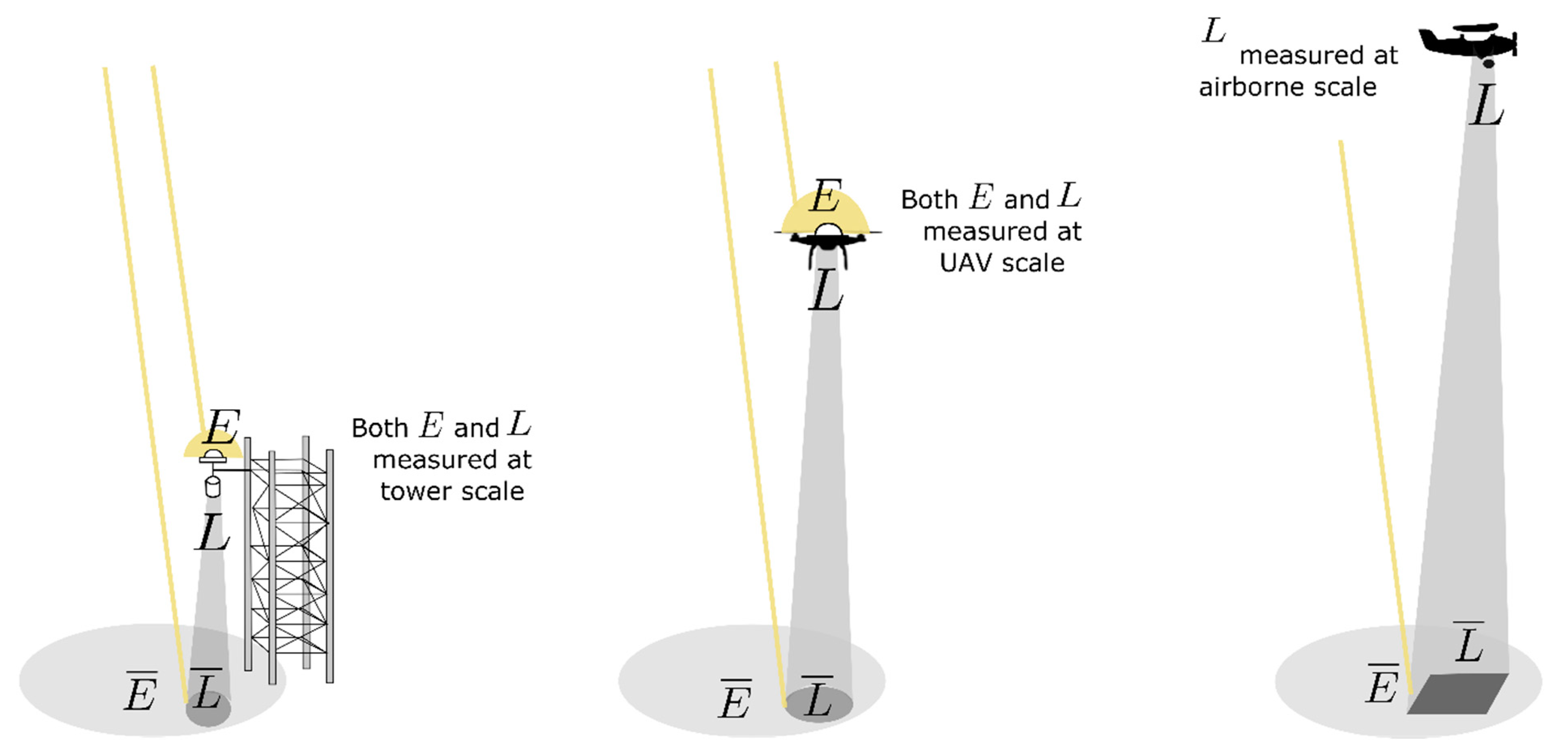
4.4. Influence of the Spatial Measurement Scale

When current in situ approaches and protocols (cf. Section 3) are applied, temporally continuous but spatially discrete stationary F measurements can achieve reliable results. However, the representativeness of spatially discrete measurements of larger areas or the whole landscape is often limited. Consequently, the spatial extrapolation of discrete observations is hampered by the concurrent and compounding effects of the vegetation structure and composition, topography, and canopy morphology and the intrinsic spatial variability in vegetation canopies. The spatial composition of differently behaving plants or land cover types increases the complexity. Spatial heterogeneity can thus compromise a chosen sampling design for field measurements that should ideally represent surface variation and not local variations around the location of the instrument. Consequently, cross-scale assessments and comparisons of F require the consideration of spatial heterogeneity to adequately select sampling schemes (e.g., location of measurement, spatial extent to be measured) and properly operate field and airborne spectroradiometers [147,148]. Additionally, the combined analysis of spatial heterogeneity for individual traits with theoretically expected covariances of traits would enable the identification of the superimposing effects in retrieved trait information (e.g., insufficiently compensated canopy structural effects during F retrievals) [76,125].
Another spatial scaling effect that matters is the choice of the ground sampling distance since the composition of plants and land cover types in the sensor’s field of view determines the pixel-wise retrieved trait information (e.g., F, chlorophyll content). For instance, the authors of [93] used high spatial resolution (0.4 m) UAV hyperspectral imagery with a relatively low spectral resolution (6.4 nm FWHM) to approximate F760 using the FLD method from pure tree crown and aggregated pixels (50 m). They found that only a poor relationship is evident between pure crown F and F for aggregated trees, including crowns, shadows, and background. Similar results were found in [149], in which the authors investigated the effect of spatial resolution (aggregation) with the FluorFLIGHT RTM using the high-resolution (0.6 m) hyperspectral data of an oak forest study site and 3FLD. They concluded that the F signal retrieved from mixed pixels was significantly affected by illumination effects and the canopy structure. Those effects are intrinsic to all radiance spectra retrieved from aggregated pixels, irrespective of the sample size, and they become increasingly critical with increasing levels of aggregation (pixel size) [89]. Further research is needed to investigate the spatial distribution of F in heterogeneous environments, along with the interaction of different traits (and what we can learn from it) and the right measurement scale to understand the physiological processes and their interaction.

4.5. Computer Models’ Bridging Scales

Since laboratory and field scaling experiments are time-consuming and expensive, computer models for the radiative transfer of F emitted from PSI and PSII to the tops and bottoms of leaves and to the top of the canopy have been developed to facilitate this task. The first attempts to model F on both leaf and canopy levels were undertaken in [150], which built upon the Kubelka–Munk (KM) two-stream radiative transfer theory. The recently developed leaf-level chlorophyll fluorescence model FLUSPECT [64], being a ´clone´ of the PROSPECT dicotyledon leaf reflectance and transmittance model [151] is also based on the KM theory. FLUSPECT was, for the purpose of canopy modeling efforts, coupled with the radiative transfer and energy balance model entitled ‘Soil Canopy Observation, Photochemistry and Energy fluxes’ (SCOPE; [152]), which originates from the four-stream ‘Scattering of Arbitrarily Inclined Leaves’ (SAIL) model of Verhoef [153]. Both models, SAIL and SCOPE, belong to the category of one-dimensional models and enable the scaling of leaf optical properties, including F, through canopies represented by a homogeneous turbid medium of leaves. A new SCOPE extension, called mSCOPE [154] enables modeling F from several optically distinct superimposed homogeneous leaf layers, but it cannot reproduce architecturally distinct canopies consisting of several structurally different plant functional types. F of such complex canopies can be simulated with three-dimensional models, such as the Discrete Anisotropic Radiative Transfer (DART; [155]), the FluorFLIGHT model [149], or the Fluorescence model with Weight Photon Spread (FluorWPS; [156]). Although these models were designed specifically to scale F signals across spatial scales, while accounting for various canopy structures and solar illumination-canopy-sensor geometries, they are still mathematical constructs of simplified reality and cannot be fully trusted. Nonetheless, they can provide unique insights into the sensitivity of top-of-canopy F to various structural and spectral properties, which would be difficult to unambiguously identify via experimental measurements and can thus also help to identify important ancillary data. Additionally, it is important to note that, similar to the requirements for measurements, it is necessary to register the priors (field or literature-based) and boundary conditions of the model as metadata when using these models, to be able to reproduce the results. Uncertainty (quality flags) and representativeness indicators (n) for model parametrization should also be documented.

5. Summary and Discussion

Within the last decade, research on F has intensified. The announcement of FLEX as the next ESA Earth Explorer mission [157] has triggered the development of dedicated instrumentation and protocols. These advancements have improved the reliability of spectroradiometric measurements and eventually enabled the measurement of subtle F signals with well-calibrated and temperature-stabilized [38] this issue state-of-the-art spectroradiometers for operation at the leaf and canopy level. Still, highly reliable radiance measurements of F require not only further technological development, but also the sufficient precision of measurements, correct setups, and well-postulated measurement protocols.
The current trend of instrumentation is moving toward a higher spectral resolution and a high signal-to-noise ratio (SNR). While spectroradiometers with an FWHM of a few nanometers may allow one to estimate F760, only actively cooled sensors (enabling high SNR at a very high spectral resolution (FWHM < 1 nm), e.g., the QE Pro spectroradiometer (OceanOptics, Inc., Dunedin, FL, USA) offer the ability to retrieve F in both atmospheric oxygen bands (i.e., F760 and F687). Point spectroradiometers with such a configuration are used for ground- and tower-based measurements as well as UAV setups. Imaging systems with a very high resolution and SNR are barely available. This poses particular challenges when investigating the spatial F dynamics. Although some measurement setups are yet able investigate different plant functional types, e.g., broadleaf forest and grassland pasture at the Majadas research site (Spain), most of the current setups monitor only one vegetation type. In addition to UAV systems, installations similar to field phenotyping platforms (e.g., [158,159]) could overcome this issue by their ability to repeatedly measure multiple points in the field in an automated fashion. Canopy F emissions are modulated by several external environmental factors, such as incoming PAR, air temperature, and wind, in combination with plant-specific traits, e.g., canopy chlorophyll content and architecture and the actual status of physiological processes [72]. Hence, more studies investigating the spatial distribution of F for multi-species canopies and research aiming to link temporal continuous measurements with spatial continuous measurements are needed. Such studies must consider all issues related to the comparability of imaging and non-imaging data and different reflectance factors (hemispherical–conical vs. hemispherical–directional), such as those outlined in [13,80].
Standardization of measurement protocols has been mostly advanced by standardizing F-measuring systems, resulting in systems such as the FluoWat, FloX, and Piccolo. Also, measurement setups have become more robust. The current continuous ground-based measurements enable investigations of F temporal dynamics under real environmental conditions. This is important for not only getting a deeper insight into plant physiological processes but also understanding temporally discrete F observations, such as those from airborne platforms and current and future spaceborne missions. Temporally continuous measurement setups should be extended with auxiliary information, which is necessary to interpret the F signal correctly. It is important to mention that current continuous measurements usually cover only a small area (most of the time, only one discrete point in space). Larger areas could be characterized by discrete overflights of airborne systems, but carrying out an airborne campaign requires more efforts and planning compared with fixed-ground and tower-based installations. Moreover, one needs to think about the extrapolation of airborne observations through time. Regarding flexibility, leaf clip F measurements on single leaves are easy to carry out since the logistics and organizational efforts are low. Yet, they require a lot of human interactions and provide only a limited number of measurements at a given time. In contrast, constantly measuring fixed-sensor installations are very inflexible when it comes to measuring different places, but they remove the need for human operators. Table 1 summarizes F measurement considerations. Future research should investigate how different approaches and their advantages and disadvantages can be combined in a meaningful way to get the full F picture at various spatial and temporal scales.
However, it is not only the technology and measurement setups that vary at different levels and scales. The review of different measurement protocols showed that differences also exist between F retrieval approaches. The most apparent difference between the leaf level and the canopy level is the ability to use a sharp-edge low-pass filter to cut off photosynthetically active light, as well as to measure both leaf upwelling and downwelling F radiation. This simplifies the retrieval of F, because it does not require disentangling the signal from the reflected or transmitted F radiance. With canopy-level measurements, the photon scattering and reabsorption further complicate the F estimation. Also, the different approaches have different temporal frequencies and continuities and are thus able to measure physiological processes to different extents.
One of the open issues is the influence of the measurement geometry. It has been shown that measurement geometries influence radiance measurements and, consequently, also the retrieved biophysical parameters [106,108]. Several studies [76,82,160] have reported that the anisotropy of F emissions is related to the canopy structure, and this relationship implies that the sensor viewing geometry is also important for F measurements. Thus, the comparability and standardization of nadir and oblique measurements (e.g., from towers) should be investigated, and common protocols for observations and instrumental setups should be established. Additionally, the atmosphere between the instrument and the observed canopy needs attention. While correction of an F signal recorded from less than 2 m above the top of the canopy does not seem necessary for either oxygen absorption or aerosol transmittance, even tower measurements require the correction of oxygen absorption. Some tower-based studies have already reported on such corrections [46,47], while others have not. For airborne studies, atmospheric correction is mandatory [85,87,115,158]. Nevertheless, further research on atmospheric corrections should investigate the stability of F because of the large variety in measurement setups, places, and atmospheric conditions.
Another critical point is the quality checks and quality flags present in the metadata. Not much has been reported on this topic. Proper calibration, which includes quality indicators related to the uncertainty of the measurements, and correct installation (e.g., thermal stabilization of the sensor; fixed fiber optic setup; installations to keep birds, insects, and dirt away from the reference measurement), is the cornerstones of reliable measurements. Still, constant changes in atmospheric conditions, in combination with the fast response of F to E changes and environmental stress, make it necessary to track the measurement quality and eventually omit uncertain measurements. The related suggestions discussed in Section 4.3 and Section 4.4 are considered as a starting point, but more data-driven research is needed in this direction. Similarly, it is crucial to report metadata and ancillary data, particularly for the measurement of F since it is sensitive to many confounding factors. It is expected that the ongoing research on F will reveal which additional information is necessary. It is advisable to record as many of the parameters stated in Section 4.4 as possible to improve the comparability of measurements among experiments and scales.
All of these efforts will complement traditional field spectroscopy in its role, as defined by Milton [1] 30 years ago: “Firstly, it acts as a bridge between laboratory measurements of spectral reflectance and the field situation and is thus useful in the calibration of airborne and satellite sensors. Secondly, it is useful in predicting the optimum spectral bands, viewing configuration and time to perform a particular remote sensing task. Thirdly, it provides a tool for the development, refinement, and testing of models relating biophysical attributes to remotely-sensed data” [1]. A crucial step is to investigate how measurements on different scales can complement each other and be combined to gain ecosystem-wide insights. Since laboratory and field scaling experiments are laborious and possibly insufficient to address the complexity and dynamics of the underlying processes determining variations in F, the refinement and use of (3D) radiative transfer models will play a crucial role in facilitating such scaling research.

6. Conclusions

Substantial progress has been made in the last 10 years in the passive measurement of F data. Besides the remarkable advancements in technology, more sophisticated measurement setups and protocols have also been defined and implemented, while standardization has mainly evolved as a result of standardized systems, such as the FluoWat, FloX, and Piccolo. Future steps should aim to incorporate atmospheric correction as well as implement standardized quality checks and flags in the data by default. This also involves tracking metadata and ancillary data to improve the interpretation and further use of F data. Besides instrumental and data science, more research is also needed on the comparability and transferability of results from different experiments across spatial and temporal scales. Such research needs can be supported by combining observational results with virtual ecosystems obtained from computer models. The scenarios should include the effects of diversity in plant functional traits across vegetation types and should be able to describe heterogeneous landscapes. All of these steps are necessary to facilitate the synthesis of activities and to move beyond single sites and single campaigns. Since these topics are too complex to be addressed by individual researchers, we hope that the promising collaborations between researchers will continue and allow the community to identify and implement solutions to these challenges.

Supplementary Materials

The following are available online at: https://0-www-mdpi-com.brum.beds.ac.uk/2072-4292/11/8/927/s1; Figure S1: Diurnal photosynthetic photon flux density (PPFD; red line) and relative standard deviation of fluorescence at 760 nm (F760; black cycles) for a sunny day with few clouds (A) and a cloudy day with strong cloud cover (B). Measurements were taken with a QE Pro over sugar beet on 20.08.2015 (A) and 30.07.2015 (B), Merzenhausen, Germany. The spectroradiometer system has a spectral resolution of 1 nm FWHM (full-width at half maximum), a spectral sampling interval (SI) of 0.3 nm, and a signal-to-noise ratio (SNR) of 1000:1 in a spectral range from 300 to 1000 nm. Measurements were taken every 6–8 seconds; Figure S2: Diurnal photosynthetic photon flux density (PPFD; red line) and relative standard deviation of fluorescence at 760 nm (F760; black cycles) for a sunny day with few clouds (A) and a cloudy day with strong cloud cover (B) after using a 1% illumination filter. Measurements were taken with a QE Pro over sugar beet on 20.08.2015 (A) and 30.07.2015 (B), Merzenhausen, Germany. The spectroradiometer system has a spectral resolution of 1 nm FWHM (full-width at half maximum), a spectral sampling interval (SI) of 0.3 nm, and a signal-to-noise ratio (SNR) of 1000:1 in a spectral range from 300 to 1000 nm. Measurements were taken every 6–8 seconds, Figure S3: Boxplot of the relative standard deviation (RSD) of fluorescence at 760 and 687 nm (F760 and F687) for four different illumination quality filters. The dataset was measured over 65 days from June to August 2015 within a sugar beet field in Merzenhausen, Germany. The quality filter labeled “none” does not consider illumination changes between two measurement cycles (6–8 s), the quality filters 10%, 1%, and 0.1% discard samples that show an illumination change of 10, 1, 0.1% between two measurement cycles, respectively. The green bar in the Boxplot shows the median value, the whiskers show the minimum and maximum RSD, the lower box border shows the first quartile, and the upper box border the third quartile, Table S1: Proposed metadata attributes for spectroradiometric data for F retrieval grouped by metadata categories, with core attributes shaded in gray and justification for their inclusion in the F metadata set. Attributes or metadata categories that are not yet included in the SPECCHIO metadata model are indicated with an asterisk*, Table S2: Instruments used to measure F.

Author Contributions

H.A., M.P.C.-M., J.P.-L., A.M.A. and various members the OPTIMISE community conceptualized the three papers on measuring sun-induced chlorophyll fluorescence. H.A. coordinated the work on this manuscript and wrote the majority of Section 1, Section 5, and Section 6. Section 2 was coordinated and written by Y.G. and S.V.W. Section 3.1 was coordinated and majorly written by S.V.W. with input from L.A. Section 3.2 was mostly written by H.A. with input from J.P-L., A.B., S.C., and E.T. Section 4.1 was written by N.S.M. Section 4.2 was written by S.W. Section 4.3. was coordinated by S.V.W. and A.H. and written by S.V.W., A.H., and N.S.M. Section 4.4 was written by A.D. with contributions from H.A. Section 4.5 was written by Z.M. All authors provided contributions to various parts of the manuscript. A.D., Y.G., A.M.A., U.R., S.W., S.V.W., Z.M., L.A., and H.A. reviewed and edited large parts of the manuscript.

Funding

This article is based upon work from COST Action ESSEM COST Action ES1309 OPTIMISE supported by COST (European Cooperation in Science and Technology, www.cost.eu). Van Wittenberghe S. was funded by the European Union’s H2020 Marie Skłodowska-Curie individual fellowship under the grant agreement FLUOPHOT (no. 701815) and is currently funded by the Generalitat Valenciana (APOSTD/2018/162) postdoctoral scholarship co-funded by the ‘Fondo Social Europeo’. Cendrero-Mateo M.P. is currently funded by AVANFLEX project (Advanced Products for the FLEX mission), no. ESP2016-79503-C2-1-P, Ministry of Economy and Competitiveness, Spain. Goulas Y. is currently funded by the ECOFLUO project (In-situ Remote Sensing of Chlorophyll Fluorescence to Monitor Carbon Dynamics in Ecosystems in support of the FLEX mission), no. 4500058116 and 4500058229, Centre National d’Etudes Spatiales (CNES), France. Zbynĕk Malenovský is supported by the Australian Research Council Future Fellowship: Bridging Scales in Remote Sensing of Vegetation Stress (FT160100477). Mac Arthur, A. was funded by the UK NERC/NCEO through the Field Spectroscopy Facility at GeoSciences, University of Edinburgh. Wieneke, S. is currently funded by the individual fellowship of the European Union’s H2020 Marie Skłodowska-Curie actions under the grant agreement ReSPEc (no. 795299). The contributions by Andreas Hueni were supported by the University of Zurich Priority Programme on Global Change and Biodiversity (URPP GCB) and by the MetEOC project in the frameworks of EMRP and EMPIR supported by the European Union. Many experimental studies were supported by the European Space Agency ESA in the framework of field campaigns supporting the FLEX satellite mission, such as the HyFLEX campaign (ESA contract no. 4000107143/12/NL/FF/If CCN3), the AtmoFLEX campaign, or the FLEXSense campaign (ESA contract no. ESA RFP/3-15477/18/NL/NA). Pacheco-Labrador, J. was supported by the EnMAP project MoReDEHESHyReS “Modelling Responses of Dehesas with Hyperspectral Remote Sensing” (contract no. 50EE1621, German Aerospace Center (DLR) and the German Federal Ministry of Economic Affairs and Energy) and the Alexander von Humboldt Foundation via Max-Planck Prize to Markus Reichstein.

Acknowledgments

We are deeply thankful to all members of the ESSEM COST Action ES1309 OPTIMISE for many stimulating meetings that helped to develop the science and formed networks of collaborators and friends. This was made possible through the funding and support of COST (https://www.cost.eu), which we gratefully acknowledge. Moreover, we would specifically like to thank all the local organizers of workshops, teachers, working group leaders, core group members, and others that helped to keep OPTIMISE running. Furthermore, we also thank our research groups that allowed us to spend time on the activities related to OPTIMISE. Also, we acknowledge Julianne Bending for providing Figure 5b. Finally, yet importantly, we thank the three anonymous reviewers that helped to improve the manuscript.

Conflicts of Interest

The authors declare no conflicts of interest.

References

  1. Milton, E.J. Principles of field spectroscopy. Int. J. Remote Sens. 1987, 8, 1807–1827. [Google Scholar] [CrossRef]
  2. Goetz, A.F.H.; Vane, G.; Solomon, J.E.; Rock, B.N. Imaging Spectrometry for Earth Remote Sensing. Science 1985, 228, 1147–1153. [Google Scholar] [CrossRef] [PubMed]
  3. Milton, E.J.; Schaepman, M.E.; Anderson, K.; Kneubühler, M.; Fox, N. Progress in field spectroscopy. Remote Sens. Environ. 2009, 113, S92–S109. [Google Scholar] [CrossRef]
  4. Goetz, A.F.H. Three decades of hyperspectral remote sensing of the Earth: A personal view. Remote Sens. Environ. 2009, 113, S5–S16. [Google Scholar] [CrossRef]
  5. Agati, G. Response of thein vivochlorophyll fluorescence spectrum to environmental factors and laser excitation wavelength. Pure Appl. Opt. 1998, 7, 797–807. [Google Scholar] [CrossRef]
  6. Cendrero-Mateo, M.P.; Moran, M.S.; Papuga, S.A.; Thorp, K.R.; Alonso, L.; Moreno, J.; Ponce-Campos, G.; Rascher, U.; Wang, G. Plant chlorophyll fluorescence: Active and passive measurements at canopy and leaf scales with different nitrogen treatments. J. Exp. Bot. 2016, 67, 275–286. [Google Scholar] [CrossRef] [PubMed]
  7. Van Wittenberghe, S.; Alonso, L.; Verrelst, J.; Hermans, I.; Valcke, R.; Veroustraete, F.; Moreno, J.; Samson, R. A field study on solar-induced chlorophyll fluorescence and pigment parameters along a vertical canopy gradient of four tree species in an urban environment. Sci. Total Environ. 2014, 466–467, 185–194. [Google Scholar] [CrossRef]
  8. Yang, X.; Tang, J.; Mustard, J.F.; Lee, J.-E.; Rossini, M.; Joiner, J.; Munger, J.W.; Kornfeld, A.; Richardson, A.D. Solar-induced chlorophyll fluorescence that correlates with canopy photosynthesis on diurnal and seasonal scales in a temperate deciduous forest. Geophys. Res. Lett. 2015, 42, 2977–2987. [Google Scholar] [CrossRef]
  9. Pinto, F.; Damm, A.; Schickling, A.; Panigada, C.; Cogliati, S.; Müller-Linow, M.; Balvora, A.; Rascher, U. Sun-induced chlorophyll fluorescence from high-resolution imaging spectroscopy data to quantify spatio-temporal patterns of photosynthetic function in crop canopies: Sun-induced fluorescence in crop canopies. Plant Cell Environ. 2016, 39, 1500–1512. [Google Scholar] [CrossRef]
  10. Cogliati, S.; Rossini, M.; Julitta, T.; Meroni, M.; Schickling, A.; Burkart, A.; Pinto, F.; Rascher, U.; Colombo, R. Continuous and long-term measurements of reflectance and sun-induced chlorophyll fluorescence by using novel automated field spectroscopy systems. Remote Sens. Environ. 2015, 164, 270–281. [Google Scholar] [CrossRef]
  11. Daumard, F.; Champagne, S.; Fournier, A.; Goulas, Y.; Ounis, A.; Hanocq, J.F.; Moya, I. A Field Platform for Continuous Measurement of Canopy Fluorescence. IEEE Trans. Geosci. Remote Sens. 2010, 48, 3358–3368. [Google Scholar] [CrossRef]
  12. Aasen, H.; Honkavaara, E.; Lucieer, A.; Zarco-Tejada, P.J. Quantitative Remote Sensing at Ultra-High Resolution with UAV Spectroscopy: A Review of Sensor Technology, Measurement Procedures, and Data Correction Workflows. Remote Sens. 2018, 10, 1091. [Google Scholar] [CrossRef]
  13. Aasen, H.; Bolten, A. Multi-temporal high-resolution imaging spectroscopy with hyperspectral 2D imagers – From theory to application. Remote Sens. Environ. 2018, 205, 374–389. [Google Scholar] [CrossRef]
  14. Garzonio, R.; Mauro, B.D.; Colombo, R.; Cogliati, S. Surface Reflectance and Sun-Induced Fluorescence Spectroscopy Measurements Using a Small Hyperspectral UAS. Remote Sens. 2017, 9, 472. [Google Scholar] [CrossRef]
  15. Adão, T.; Hruška, J.; Pádua, L.; Bessa, J.; Peres, E.; Morais, R.; Sousa, J. Hyperspectral Imaging: A Review on UAV-Based Sensors, Data Processing and Applications for Agriculture and Forestry. Remote Sens. 2017, 9, 1110. [Google Scholar] [CrossRef]
  16. Zarco-Tejada, P.J.; González-Dugo, V.; Berni, J.A.J. Fluorescence, temperature and narrow-band indices acquired from a UAV platform for water stress detection using a micro-hyperspectral imager and a thermal camera. Remote Sens. Environ. 2012, 117, 322–337. [Google Scholar] [CrossRef]
  17. MacArthur, A.; Robinson, I.; Rossini, M.; Davis, N.; MacDonald, K. A dual-field-of-view spectrometer system for reflectance and fluorescence measurements (Piccolo Doppio) and correction of etaloning. In Proceedings of the 5th International Workshop on Remote Sensing of Vegetation Fluorescence, Paris, France, 22–24 April 2014; European Space Agency: Paris, France, 2014. [Google Scholar]
  18. Tomelleri, E.; Mejia-Aguilar, A. Inversion of the Prosail Model from UAV Data. In Proceedings of the 2018 IEEE International Geoscience and Remote Sensing Symposium (IGARSS), Valencia, Spain, 22–27 July 2018; pp. 8813–8815. [Google Scholar]
  19. Rascher, U.; Alonso, L.; Burkart, A.; Cilia, C.; Cogliati, S.; Colombo, R.; Damm, A.; Drusch, M.; Guanter, L.; Hanus, J.; et al. Sun-induced fluorescence—A new probe of photosynthesis: First maps from the imaging spectrometer HyPlant. Glob. Chang. Biol. 2015, 21, 4673–4684. [Google Scholar] [CrossRef]
  20. Schaepman, M.E.; Jehle, M.; Hueni, A.; D’Odorico, P.; Damm, A.; Weyermann, J.; Schneider, F.D.; Laurent, V.; Popp, C.; Seidel, F.C.; et al. Advanced radiometry measurements and Earth science applications with the Airborne Prism Experiment (APEX). Remote Sens. Environ. 2015, 158, 207–219. [Google Scholar] [CrossRef]
  21. Green, R.O.; Eastwood, M.L.; Sarture, C.M.; Chrien, T.G.; Aronsson, M.; Chippendale, B.J.; Faust, J.A.; Pavri, B.E.; Chovit, C.J.; Solis, M.; et al. Imaging Spectroscopy and the Airborne Visible/Infrared Imaging Spectrometer (AVIRIS). Remote Sens. Environ. 1998, 65, 227–248. [Google Scholar] [CrossRef]
  22. Belward, A.S.; Skøien, J.O. Who launched what, when and why; trends in global land-cover observation capacity from civilian earth observation satellites. ISPRS J. Photogramm. Remote Sens. 2015, 103, 115–128. [Google Scholar] [CrossRef]
  23. Joiner, J.; Yoshida, Y.; Guanter, L.; Middleton, E.M. New methods for the retrieval of chlorophyll red fluorescence from hyperspectral satellite instruments: Simulations and application to GOME-2 and SCIAMACHY. Atmos. Meas. Tech. 2016, 9, 3939–3967. [Google Scholar] [CrossRef]
  24. Guanter, L.; Zhang, Y.; Jung, M.; Joiner, J.; Voigt, M.; Berry, J.A.; Frankenberg, C.; Huete, A.R.; Zarco-Tejada, P.; Lee, J.-E.; et al. Global and time-resolved monitoring of crop photosynthesis with chlorophyll fluorescence. Proc. Natl. Acad. Sci. USA 2014, 111, E1327–E1333. [Google Scholar] [CrossRef]
  25. Guanter, L.; Frankenberg, C.; Dudhia, A.; Lewis, P.E.; Gómez-Dans, J.; Kuze, A.; Suto, H.; Grainger, R.G. Retrieval and global assessment of terrestrial chlorophyll fluorescence from GOSAT space measurements. Remote Sens. Environ. 2012, 121, 236–251. [Google Scholar] [CrossRef]
  26. Frankenberg, C.; Butz, A.; Toon, G.C. Disentangling chlorophyll fluorescence from atmospheric scattering effects in O2 A-band spectra of reflected sun-light. Geophys. Res. Lett. 2011, 38. [Google Scholar] [CrossRef]
  27. Joiner, J.; Yoshida, Y.; Vasilkov, A.P.; Corp, L.A.; Middleton, E.M. First observations of global and seasonal terrestrial chlorophyll fluorescence from space. Biogeosciences 2011, 8, 637–651. [Google Scholar] [CrossRef]
  28. Baker, N.R. Chlorophyll fluorescence: A probe of photosynthesis in vivo. Annu. Rev. Plant Biol. 2008, 59, 89–113. [Google Scholar] [CrossRef]
  29. Maxwell, K.; Johnson, G.N. Chlorophyll fluorescence—A practical guide. J. Exp. Bot. 2000, 51, 659–668. [Google Scholar] [CrossRef]
  30. Kolber, Z.; Klimov, D.; Ananyev, G.; Rascher, U.; Berry, J.; Osmond, B. Measuring photosynthetic parameters at a distance: Laser induced fluorescence transient (LIFT) method for remote measurements of photosynthesis in terrestrial vegetation. Photosynth. Res. 2005, 84, 121–129. [Google Scholar] [CrossRef]
  31. Ounis, A.; Evain, S.; Flexas, J.; Tosti, S.; Moya, I. Adaptation of a PAM-fluorometer for remote sensing of chlorophyll fluorescence. Photosynth. Res. 2001, 68, 113. [Google Scholar] [CrossRef]
  32. Hoge, F.E.; Swift, R.N. Airborne simultaneous spectroscopic detection of laser-induced water Raman backscatter and fluorescence from chlorophyll a and other naturally occurring pigments. Appl. Opt. 1981, 20, 3197–3205. [Google Scholar] [CrossRef]
  33. Keller, B.; Vass, I.; Matsubara, S.; Paul, K.; Jedmowski, C.; Pieruschka, R.; Nedbal, L.; Rascher, U.; Muller, O. Maximum fluorescence and electron transport kinetics determined by light-induced fluorescence transients (LIFT) for photosynthesis phenotyping. Photosynth. Res. 2018. [Google Scholar] [CrossRef] [PubMed]
  34. Balzarolo, M.; Anderson, K.; Nichol, C.; Rossini, M.; Vescovo, L.; Arriga, N.; Wohlfahrt, G.; Calvet, J.-C.; Carrara, A.; Cerasoli, S.; et al. Ground-based optical measurements at European flux sites: A review of methods, instruments and current controversies. Sensors 2011, 11, 7954–7981. [Google Scholar] [CrossRef] [PubMed]
  35. Gamon, J.A.; Rahman, A.F.; Dungan, J.L.; Schildhauer, M.; Huemmrich, K.F. Spectral Network (SpecNet)—What is it and why do we need it? Remote Sens. Environ. 2006, 103, 227–235. [Google Scholar] [CrossRef]
  36. Eklundh, L.; Jin, H.; Schubert, P.; Guzinski, R.; Heliasz, M. An optical sensor network for vegetation phenology monitoring and satellite data calibration. Sensors 2011, 11, 7678–7709. [Google Scholar] [CrossRef] [PubMed]
  37. Hufkens, K.; Filippa, G.; Cremonese, E.; Migliavacca, M.; D’Odorico, P.; Peichl, M.; Gielen, B.; Hörtnagl, L.; Soudani, K.; Papale, D.; et al. Assimilating phenology datasets automatically across ICOS ecosystem stations. Int. Agrophys. 2018, 32, 677–687. [Google Scholar] [CrossRef]
  38. Pacheco-Labrador, J.; Hueni, A.; Mihai, L.; Sakowska, K.; Julitta, T.; Kuusk, J.; Sporea, D.; Alonso, L.; Burkart, A.; Cendrero-Mateo, M.P.; et al. Sun-induced chlorophyll fluorescence I: Instrumental considerations for proximal spectroradiometers. Remote Sens. 2019, 11, 960. [Google Scholar] [CrossRef]
  39. Cendrero-Mateo, M.P.; Wieneke, S.; Damm, A.; Alonso, L.; Pinto, F.; Moreno, J.; Guanter, L.; Celesti, M.; Rossini, M.; Sabater, N.; et al. Sun-induced chlorophyll fluorescence III: Benchmarking retrieval methods and sensor characteristics for proximal sensing. Remote Sens. 2019, 11, 962. [Google Scholar] [CrossRef]
  40. Meroni, M.; Rossini, M.; Guanter, L.; Alonso, L.; Rascher, U.; Colombo, R.; Moreno, J. Remote sensing of solar-induced chlorophyll fluorescence: Review of methods and applications. Remote Sens. Environ. 2009, 113, 2037–2051. [Google Scholar] [CrossRef]
  41. Sun, Y.; Frankenberg, C.; Jung, M.; Joiner, J.; Guanter, L.; Köhler, P.; Magney, T. Overview of Solar-Induced chlorophyll Fluorescence (SIF) from the Orbiting Carbon Observatory-2: Retrieval, cross-mission comparison, and global monitoring for GPP. Remote Sens. Environ. 2018, 209, 808–823. [Google Scholar] [CrossRef]
  42. Demmig-Adams, B.; Cohu, C.M.; Muller, O.; Adams, W.W., 3rd. Modulation of photosynthetic energy conversion efficiency in nature: From seconds to seasons. Photosynth. Res. 2012, 113, 75–88. [Google Scholar] [CrossRef]
  43. Lichtenthaler, H.K.; Rinderle, U. The Role of Chlorophyll Fluorescence in the Detection of Stress Conditions in Plants. Crit. Rev. Anal. Chem. 1988, 19, S29–S85. [Google Scholar] [CrossRef]
  44. Louis, J.; Cerovic, Z.G.; Moya, I. Quantitative study of fluorescence excitation and emission spectra of bean leaves. J. Photochem. Photobiol. B 2006, 85, 65–71. [Google Scholar] [CrossRef]
  45. Rossini, M.; Meroni, M.; Celesti, M.; Cogliati, S.; Julitta, T.; Panigada, C.; Rascher, U.; van der Tol, C.; Colombo, R. Analysis of Red and Far-Red Sun-Induced Chlorophyll Fluorescence and Their Ratio in Different Canopies Based on Observed and Modeled Data. Remote Sens. 2016, 8, 412. [Google Scholar] [CrossRef]
  46. Goulas, Y.; Fournier, A.; Daumard, F.; Champagne, S.; Ounis, A.; Marloie, O.; Moya, I. Gross Primary Production of a Wheat Canopy Relates Stronger to Far Red Than to Red Solar-Induced Chlorophyll Fluorescence. Remote Sens. 2017, 9, 97. [Google Scholar] [CrossRef]
  47. Daumard, F.; Goulas, Y.; Champagne, S.; Fournier, A.; Ounis, A.; Olioso, A.; Moya, I. Continuous Monitoring of Canopy Level Sun-Induced Chlorophyll Fluorescence During the Growth of a Sorghum Field. IEEE Trans. Geosci. Remote Sens. 2012, 50, 4292–4300. [Google Scholar] [CrossRef]
  48. Plascyk, J.A. The MK II Fraunhofer Line Discriminator (FLD-II) for Airborne and Orbital Remote Sensing of Solar-Stimulated Luminescence. Organ. Ethic. 1975, 14, 144339. [Google Scholar] [CrossRef]
  49. Plascyk, J.A.; Gabriel, F.C. The Fraunhofer Line Discriminator MKII-An Airborne Instrument for Precise and Standardized Ecological Luminescence Measurement. IEEE Trans. Instrum. Meas. 1975, 24, 306–313. [Google Scholar] [CrossRef]
  50. Maier, S.W.; Günther, K.P.; Stellmes, M. Sun-Induced Fluorescence: A New Tool for Precision Farming. In Digital Imaging and Spectral Techniques: Applications to Precision Agriculture and Crop Physiology; ASA Special Publication; American Society of Agronomy, Crop Science Society of America, and Soil Science Society of America: Madison, WI, USA, 2003; pp. 209–222. ISBN 9780891183327. [Google Scholar]
  51. Alonso, L.; Gomez-Chova, L.; Vila-Frances, J.; Amoros-Lopez, J.; Guanter, L.; Calpe, J.; Moreno, J. Improved Fraunhofer Line Discrimination Method for Vegetation Fluorescence Quantification. IEEE Geosci. Remote Sens. Lett. 2008, 5, 620–624. [Google Scholar] [CrossRef]
  52. Cogliati, S.; Verhoef, W.; Kraft, S.; Sabater, N.; Alonso, L.; Vicent, J.; Moreno, J.; Drusch, M.; Colombo, R. Retrieval of sun-induced fluorescence using advanced spectral fitting methods. Remote Sens. Environ. 2015, 169, 344–357. [Google Scholar] [CrossRef]
  53. Meroni, M.; Busetto, L.; Colombo, R.; Guanter, L.; Moreno, J.; Verhoef, W. Performance of Spectral Fitting Methods for vegetation fluorescence quantification. Remote Sens. Environ. 2010, 114, 363–374. [Google Scholar] [CrossRef]
  54. McFarlane, J.C.; Watson, R.D.; Theisen, A.F.; Jackson, R.D.; Ehrler, W.L.; Pinter, P.J.; Idso, S.B.; Reginato, R.J. Plant stress detection by remote measurement of fluorescence. Appl. Opt. 1980, 19, 3287. [Google Scholar] [CrossRef]
  55. Gitelson, A.A.; Buschmann, C.; Lichtenthaler, H.K. Leaf chlorophyll fluorescence corrected for re-absorption by means of absorption and reflectance measurements. J. Plant Physiol. 1998, 152, 283–296. [Google Scholar] [CrossRef]
  56. Rinderle, U.; Lichtenthaler, H.K. The Chlorophyll Fluorescence Ratio F690/F735 as a Possible Stress Indicator. In Applications of Chlorophyll Fluorescene in Photosynthesis Research, Stress Physiology, Hydrobiology and Remote Sensing; Lichtenthaler, H.K., Ed.; Kluwer Academic Publishers: Dordrecht, The Netherlands, 1988; pp. 189–196. [Google Scholar]
  57. Amorós-López, J.; Vila-Frances, J.; Gomez-Chova, L.; Alonso, L.; Guanter, L.; del Valle-Tascon, S.; Calpe, J.; Moreno, J. Remote sensing of chlorophyll fluorescence for estimation of stress in vegetation recommendations for future missions. In Proceedings of the 2007 IEEE International Geoscience and Remote Sensing Symposium, Barcelona, Spain, 23–28 July 2007. [Google Scholar]
  58. Alonso, L.; Van Wittenberghe, S.; Amorós-López, J.; Vila-Francés, J.; Gómez-Chova, L.; Moreno, J. Diurnal Cycle Relationships between Passive Fluorescence, PRI and NPQ of Vegetation in a Controlled Stress Experiment. Remote Sens. 2017, 9, 770. [Google Scholar] [CrossRef]
  59. Atherton, J.; Nichol, C.J.; Porcar-Castell, A. Using spectral chlorophyll fluorescence and the photochemical reflectance index to predict physiological dynamics. Remote Sens. Environ. 2016, 176, 17–30. [Google Scholar] [CrossRef]
  60. Rajewicz, P.; Atherton, J.; Alonso, L.; Porcar-Castell, A. Leaf-Level Spectral Fluorescence Measurements: Comparing Methodologies for Broadleaves and Needles. Remote Sens. 2019, 11, 532. [Google Scholar] [CrossRef]
  61. Alonso, L.; Moreno, J. A Novel Portable Device to Measure Leaf Reflectance, Transmittance and Fluorescence Emission under Natural Conditions. In Proceedings of the 4th International Workshop on Remote Sensing of Vegetation Fluorescence, Valencia, Spain, 15–17 November 2010. [Google Scholar]
  62. Van Wittenberghe, S.; Alonso, L.; Verrelst, J.; Moreno, J.; Samson, R. Bidirectional sun-induced chlorophyll fluorescence emission is influenced by leaf structure and light scattering properties—A bottom-up approach. Remote Sens. Environ. 2015, 158, 169–179. [Google Scholar] [CrossRef]
  63. Van Wittenberghe, S.; Alonso, L.; Verrelst, J.; Hermans, I.; Delegido, J.; Veroustraete, F.; Valcke, R.; Moreno, J.; Samson, R. Upward and downward solar-induced chlorophyll fluorescence yield indices of four tree species as indicators of traffic pollution in Valencia. Environ. Pollut. 2013, 173, 29–37. [Google Scholar] [CrossRef]
  64. Vilfan, N.; Van der Tol, C.; Yang, P.; Wyber, R.; Malenovský, Z.; Robinson, S.A.; Verhoef, W. Extending Fluspect to simulate xanthophyll driven leaf reflectance dynamics. Remote Sens. Environ. 2018, 211, 345–356. [Google Scholar] [CrossRef]
  65. Magney, T.S.; Frankenberg, C.; Fisher, J.B.; Sun, Y.; North, G.B.; Davis, T.S.; Kornfeld, A.; Siebke, K. Connecting active to passive fluorescence with photosynthesis: A method for evaluating remote sensing measurements of Chl fluorescence. New Phytol. 2017, 215, 1594–1608. [Google Scholar] [CrossRef]
  66. Van Wittenberghe, S.; Alonso, L.; Malenovský, Z.; Moreno, J. In vivo photoprotection mechanisms observed from leaf hyperspectral absorbance changes showing the VIS-NIR slow-induced energy-independent conformational pigment bed changes. Photsynth. Res. in review.
  67. Rosema, A.; Snel, J.F.H.; Zahn, H.; Buurmeijer, W.F.; Van Hove, L.W.A. The Relation between Laser-Induced Chlorophyll Fluorescence and Photosynthesis. Remote Sens. Environ. 1998, 65, 143–154. [Google Scholar] [CrossRef]
  68. Porcar-Castell, A.; Tyystjärvi, E.; Atherton, J.; van der Tol, C.; Flexas, J.; Pfündel, E.E.; Moreno, J.; Frankenberg, C.; Berry, J.A. Linking chlorophyll a fluorescence to photosynthesis for remote sensing applications: Mechanisms and challenges. J. Exp. Bot. 2014, 65, 4065–4095. [Google Scholar] [CrossRef]
  69. Ocean Optics Ocean Optics. Available online: https://oceanoptics.com/ (accessed on 8 February 2018).
  70. Yang, H.; Yang, X.; Zhang, Y.; Heskel, M.A.; Lu, X.; Munger, J.W.; Sun, S.; Tang, J. Chlorophyll fluorescence tracks seasonal variations of photosynthesis from leaf to canopy in a temperate forest. Glob. Chang. Biol. 2017, 23, 2874–2886. [Google Scholar] [CrossRef]
  71. Guanter, L.; Rossini, M.; Colombo, R.; Meroni, M.; Frankenberg, C.; Lee, J.-E.; Joiner, J. Using field spectroscopy to assess the potential of statistical approaches for the retrieval of sun-induced chlorophyll fluorescence from ground and space. Remote Sens. Environ. 2013, 133, 52–61. [Google Scholar] [CrossRef]
  72. Migliavacca, M.; Perez-Priego, O.; Rossini, M.; El-Madany, T.S.; Moreno, G.; van der Tol, C.; Rascher, U.; Berninger, A.; Bessenbacher, V.; Burkart, A.; et al. Plant functional traits and canopy structure control the relationship between photosynthetic CO2 uptake and far-red sun-induced fluorescence in a Mediterranean grassland under different nutrient availability. New Phytol. 2017, 214, 1078–1091. [Google Scholar] [CrossRef]
  73. Rossini, M.; Nedbal, L.; Guanter, L.; Ač, A.; Alonso, L.; Burkart, A.; Cogliati, S.; Colombo, R.; Damm, A.; Drusch, M.; et al. Red and far red Sun-induced chlorophyll fluorescence as a measure of plant photosynthesis. Geophys. Res. Lett. 2015, 42, 1632–1639. [Google Scholar] [CrossRef]
  74. Julitta, T.; Corp, L.; Rossini, M.; Burkart, A.; Cogliati, S.; Davies, N.; Hom, M.; Mac Arthur, A.; Middleton, E.; Rascher, U.; et al. Comparison of Sun-Induced Chlorophyll Fluorescence Estimates Obtained from Four Portable Field Spectroradiometers. Remote Sens. 2016, 8, 122. [Google Scholar] [CrossRef]
  75. Liu, L.; Liu, X.; Hu, J.; Guan, L. Assessing the wavelength-dependent ability of solar-induced chlorophyll fluorescence to estimate the GPP of winter wheat at the canopy level. Int. J. Remote Sens. 2017, 38, 4396–4417. [Google Scholar] [CrossRef]
  76. Wieneke, S.; Burkart, A.; Cendrero-Mateo, M.P.; Julitta, T.; Rossini, M.; Schickling, A.; Schmidt, M.; Rascher, U. Linking photosynthesis and sun-induced fluorescence at sub-daily to seasonal scales. Remote Sens. Environ. 2018, 219, 247–258. [Google Scholar] [CrossRef]
  77. Cheng, Y.-B.; Middleton, E.M.; Zhang, Q.; Huemmrich, K.F.; Campbell, P.K.E.; Corp, L.A.; Cook, B.D.; Kustas, W.P.; Daughtry, C.S. Integrating Solar Induced Fluorescence and the Photochemical Reflectance Index for Estimating Gross Primary Production in a Cornfield. Remote Sens. 2013, 5, 6857–6879. [Google Scholar] [CrossRef]
  78. Burkart, A.; Schickling, A.; Mateo, M.P.C.; Wrobel, T.J.; Rossini, M.; Cogliati, S.; Julitta, T.; Rascher, U. A Method for Uncertainty Assessment of Passive Sun-Induced Chlorophyll Fluorescence Retrieval Using an Infrared Reference Light. IEEE Sens. J. 2015, 15, 4603–4611. [Google Scholar] [CrossRef]
  79. Yang, X.; Shi, H.; Stovall, A.; Guan, K.; Miao, G.; Zhang, Y.; Zhang, Y.; Xiao, X.; Ryu, Y.; Lee, J.-E. FluoSpec 2-An Automated Field Spectroscopy System to Monitor Canopy Solar-Induced Fluorescence. Sensors 2018, 18, 2063. [Google Scholar] [CrossRef] [PubMed]
  80. Hueni, A.; Damm, A.; Kneubuehler, M.; Schlapfer, D.; Schaepman, M.E. Field and Airborne Spectroscopy Cross Validation—Some Considerations. IEEE J. Sel. Top. Appl. Earth Obs. Remote Sens. 2016, 10, 1117–1135. [Google Scholar] [CrossRef]
  81. Specim Specim. Available online: http://www.specim.fi/ (accessed on 8 February 2018).
  82. Pinto, F.; Müller-Linow, M.; Schickling, A.; Cendrero-Mateo, M.; Ballvora, A.; Rascher, U. Multiangular Observation of Canopy Sun-Induced Chlorophyll Fluorescence by Combining Imaging Spectroscopy and Stereoscopy. Remote Sens. 2017, 9, 415. [Google Scholar] [CrossRef]
  83. Moya, I.; Daumard, F.; Moise, N.; Ounis, A.; Goulas, Y. First airborne multiwavelength passive chlorophyll fluorescence measurements over La Mancha (Spain) fields. In Proceedings of the 2nd International Symposium on Recent Advances in Quantitative Remote Sensing: RAQRS’II, Torrent (Valencia), Spain, 25–29 September 2006. [Google Scholar]
  84. ESA. FLEX—ESA Future Missions—Earth Online—ESA. Available online: https://earth.esa.int/web/guest/missions/esa-future-missions/flex (accessed on 8 February 2018).
  85. Wieneke, S.; Ahrends, H.; Damm, A.; Pinto, F.; Stadler, A.; Rossini, M.; Rascher, U. Airborne based spectroscopy of red and far-red sun-induced chlorophyll fluorescence: Implications for improved estimates of gross primary productivity. Remote Sens. Environ. 2016, 184, 654–667. [Google Scholar] [CrossRef]
  86. Drusch, M.; Moreno, J.; Del Bello, U.; Franco, R.; Goulas, Y.; Huth, A.; Kraft, S.; Middleton, E.M.; Miglietta, F.; Mohammed, G.; et al. The FLuorescence EXplorer Mission Concept—ESA’s Earth Explorer 8. IEEE Trans. Geosci. Remote Sens. 2017, 55, 1273–1284. [Google Scholar] [CrossRef]
  87. Middleton, E.M.; Rascher, U.; Corp, L.A.; Huemmrich, K.F.; Cook, B.D.; Noormets, A.; Schickling, A.; Pinto, F.; Alonso, L.; Damm, A.; et al. The 2013 FLEX—US Airborne Campaign at the Parker Tract Loblolly Pine Plantation in North Carolina, USA. Remote Sens. 2017, 9, 612. [Google Scholar] [CrossRef]
  88. Colombo, R.; Celesti, M.; Bianchi, R.; Campbell, P.K.E.; Cogliati, S.; Cook, B.D.; Corp, L.A.; Damm, A.; Domec, J.-C.; Guanter, L.; et al. Variability of sun-induced chlorophyll fluorescence according to stand age-related processes in a managed loblolly pine forest. Glob. Chang. Biol. 2018, 24, 2980–2996. [Google Scholar] [CrossRef]
  89. Damm, A.; Guanter, L.; Verhoef, W.; Schläpfer, D.; Garbari, S.; Schaepman, M.E. Impact of varying irradiance on vegetation indices and chlorophyll fluorescence derived from spectroscopy data. Remote Sens. Environ. 2015, 156, 202–215. [Google Scholar] [CrossRef]
  90. Sun, Y.; Frankenberg, C.; Wood, J.D.; Schimel, D.S.; Jung, M.; Guanter, L.; Drewry, D.T.; Verma, M.; Porcar-Castell, A.; Griffis, T.J.; et al. OCO-2 advances photosynthesis observation from space via solar-induced chlorophyll fluorescence. Science 2017, 358. [Google Scholar] [CrossRef]
  91. Frankenberg, C.; Köhler, P.; Magney, T.S.; Geier, S.; Lawson, P.; Schwochert, M.; McDuffie, J.; Drewry, D.T.; Pavlick, R.; Kuhnert, A. The Chlorophyll Fluorescence Imaging Spectrometer (CFIS), mapping far red fluorescence from aircraft. Remote Sens. Environ. 2018, 217, 523–536. [Google Scholar] [CrossRef]
  92. Calderón, R.; Navas-Cortés, J.A.; Lucena, C.; Zarco-Tejada, P.J. High-resolution airborne hyperspectral and thermal imagery for early detection of Verticillium wilt of olive using fluorescence, temperature and narrow-band spectral indices. Remote Sens. Environ. 2013, 139, 231–245. [Google Scholar] [CrossRef]
  93. Zarco-Tejada, P.J.; Suarez, L.; Gonzalez-Dugo, V. Spatial Resolution Effects on Chlorophyll Fluorescence Retrieval in a Heterogeneous Canopy Using Hyperspectral Imagery and Radiative Transfer Simulation. IEEE Geosci. Remote Sens. Lett. 2013, 10, 937–941. [Google Scholar] [CrossRef]
  94. Zarco-Tejada, P.J.; Morales, A.; Testi, L.; Villalobos, F.J. Spatio-temporal patterns of chlorophyll fluorescence and physiological and structural indices acquired from hyperspectral imagery as compared with carbon fluxes measured with eddy covariance. Remote Sens. Environ. 2013, 133, 102–115. [Google Scholar] [CrossRef]
  95. Bendig, J.; Gautam, D.; Malenovský, Z.; Lucieer, A. Influence of Cosine Corrector and Uas Platform Dynamics on Airborne Spectral Irradiance Measurements. In Proceedings of the 2018 IEEE International Geoscience and Remote Sensing Symposium (IGARSS), Valencia, Spain, 22–27 July 2018; pp. 8822–8825. [Google Scholar]
  96. Ham, S.-H.; Kato, S.; Barker, H.W.; Rose, F.G.; Sun-Mack, S. Effects of 3-D clouds on atmospheric transmission of solar radiation: Cloud type dependencies inferred from A-train satellite data: Cloud-Type Dependent 3D Effects. J. Geophys. Res. D Atmos. 2014, 119, 943–963. [Google Scholar] [CrossRef]
  97. Bachmann, C.M.; Montes, M.J.; Parrish, C.E.; Fusina, R.A.; Nichols, C.R.; Li, R.-R.; Hallenborg, E.; Jones, C.A.; Lee, K.; Sellars, J.; et al. A dual-spectrometer approach to reflectance measurements under sub-optimal sky conditions. Opt. Express 2012, 20, 8959. [Google Scholar] [CrossRef]
  98. Anderson, K.; Milton, E.J.; Rollin, E.M. Calibration of dual-beam spectroradiometric data. Int. J. Remote Sens. 2006, 27, 975–986. [Google Scholar] [CrossRef]
  99. Meroni, M.; Barducci, A.; Cogliati, S.; Castagnoli, F.; Rossini, M.; Busetto, L.; Migliavacca, M.; Cremonese, E.; Galvagno, M.; Colombo, R.; et al. The hyperspectral irradiometer, a new instrument for long-term and unattended field spectroscopy measurements. Rev. Sci. Instrum. 2011, 82, 043106. [Google Scholar] [CrossRef]
  100. Sakowska, K.; Gianelle, D.; Zaldei, A.; MacArthur, A.; Carotenuto, F.; Miglietta, F.; Zampedri, R.; Cavagna, M.; Vescovo, L. WhiteRef: A new tower-based hyperspectral system for continuous reflectance measurements. Sensors 2015, 15, 1088–1105. [Google Scholar] [CrossRef]
  101. Mihai, L.; Mac Arthur, A.; Hueni, A.; Robinson, I.; Sporea, D. Optimized Spectrometers Characterization Procedure for Near Ground Support of ESA FLEX Observations: Part 1 Spectral Calibration and Characterisation. Remote Sens. 2018, 10, 289. [Google Scholar] [CrossRef]
  102. Sabater, N.; Middleton, E.M.; Malenovsky, Z.; Alonso, L.; Verrelst, J.; Huemmrich, K.F.; Campbell, P.K.E.; Kustas, W.P.; Vicent, J.; Van Wittenberghe, S.; et al. Oxygen transmittance correction for solar-induced chlorophyll fluorescence measured on proximal sensing: Application to the NASA-GSFC fusion tower. In Proceedings of the 2017 IEEE International Geoscience and Remote Sensing Symposium (IGARSS), Fort Worth, TX, USA, 23–28 July 2017; pp. 5826–5829. [Google Scholar]
  103. Leuning, R.; Hughes, D.; Daniel, P.; Coops, N.; Newnham, G. A multi-angle spectrometer for automatic measurement of plant canopy reflectance spectra. Remote Sens. Environ. 2006, 103, 236–245. [Google Scholar] [CrossRef]
  104. Hilker, T.; Coops, N.C.; Nesic, Z.; Wulder, M.A.; Black, A.T. Instrumentation and approach for unattended year round tower based measurements of spectral reflectance. Comput. Electron. Agric. 2007, 56, 72–84. [Google Scholar] [CrossRef]
  105. Tortini, R.; Hilker, T.; Coops, N.C.; Nesic, Z. Technological Advancement in Tower-Based Canopy xReflectance Monitoring: The AMSPEC-III System. Sensors 2015, 15, 32020–32030. [Google Scholar] [CrossRef] [PubMed]
  106. Burkart, A.; Aasen, H.; Alonso, L.; Menz, G.; Bareth, G.; Rascher, U. Angular Dependency of Hyperspectral Measurements over Wheat Characterized by a Novel UAV Based Goniometer. Remote Sens. 2015, 7, 725–746. [Google Scholar] [CrossRef]
  107. Küster, T.; Spengler, D.; Barczi, J.-F.; Segl, K.; Hostert, P.; Kaufmann, H. Simulation of Multitemporal and Hyperspectral Vegetation Canopy Bidirectional Reflectance Using Detailed Virtual 3-D Canopy Models. IEEE Trans. Geosci. Remote Sens. 2014, 52, 2096–2108. [Google Scholar] [CrossRef]
  108. Verrelst, J.; Schaepman, M.E.; Koetz, B.; Kneubühler, M. Angular sensitivity analysis of vegetation indices derived from CHRIS/PROBA data. Remote Sens. Environ. 2008, 112, 2341–2353. [Google Scholar] [CrossRef]
  109. Meroni, M.; Rossini, M.; Picchi, V.; Panigada, C.; Cogliati, S.; Nali, C.; Colombo, R. Assessing Steady-state Fluorescence and PRI from Hyperspectral Proximal Sensing as Early Indicators of Plant Stress: The Case of Ozone Exposure. Sensors 2008, 8, 1740–1754. [Google Scholar] [CrossRef]
  110. Kuusk, J. Dark Signal Temperature Dependence Correction Method for Miniature Spectrometer Modules. J. Sens. 2011, 2011, 608157. [Google Scholar] [CrossRef]
  111. Pacheco-Labrador, J.; Martín, M.P. Characterization of a field spectroradiometer for unattended vegetation monitoring. Key sensor models and impacts on reflectance. Sensors 2015, 15, 4154–4175. [Google Scholar] [CrossRef]
  112. Zarco-Tejada, P.J.; Camino, C.; Beck, P.S.A.; Calderon, R.; Hornero, A.; Hernández-Clemente, R.; Kattenborn, T.; Montes-Borrego, M.; Susca, L.; Morelli, M.; et al. Previsual symptoms of Xylella fastidiosa infection revealed in spectral plant-trait alterations. Nat. Plants 2018, 4, 432–439. [Google Scholar] [CrossRef]
  113. Berk, A.; Anderson, G.P.; Acharya, P.K.; Bernstein, L.S.; Muratov, L.; Lee, J.; Fox, M.; Adler-Golden, S.M.; Chetwynd, J.H.; Hoke, M.L.; et al. MODTRAN 5: A reformulated atmospheric band model with auxiliary species and practical multiple scattering options: Update. In Proceedings of the Algorithms and Technologies for Multispectral, Hyperspectral, and Ultraspectral Imagery XI, Orlando, FL, USA, 1 June 2005. [Google Scholar]
  114. Gueymard, C. SMARTS2, A Simple Model of the Atmospheric Radiative Transfer of Sunshine: Algorithms and Performance Assessment; Florida Solar Energy Ce nter/University of Central Florida: Cocoa, FL, USA, 1995; p. 84. [Google Scholar]
  115. Damm, A.; Guanter, L.; Laurent, V.C.E.; Schaepman, M.E.; Schickling, A.; Rascher, U. FLD-based retrieval of sun-induced chlorophyll fluorescence from medium spectral resolution airborne spectroscopy data. Remote Sens. Environ. 2014, 147, 256–266. [Google Scholar] [CrossRef]
  116. Pierluissi, J.H.; Tsai, C.M. Molecular transmittance band model for oxygen in the visible. Appl. Opt. 1986, 25, 2458–2460. [Google Scholar] [CrossRef]
  117. Sabater, N.; Vicent, J.; Alonso, L.; Verrelst, J.; Middleton, E.M.; Porcar-Castell, A.; Moreno, J. Compensation of Oxygen Transmittance Effects for Proximal Sensing Retrieval of Canopy–Leaving Sun–Induced Chlorophyll Fluorescence. Remote Sens. 2018, 10, 1551. [Google Scholar] [CrossRef]
  118. Liu, X.; Liu, L.; Hu, J.; Du, S. Modeling the Footprint and Equivalent Radiance Transfer Path Length for Tower-Based Hemispherical Observations of Chlorophyll Fluorescence. Sensors 2017, 17, 1131. [Google Scholar] [CrossRef] [PubMed]
  119. Middleton, E.; Lawrence, A.; Cook, A.B.D. FUSION: Canopy Tower System for Remote Sensing Observations of Terrestrial Ecosystems; NASA: Washington, DC, USA, 2013.
  120. Daumard, F.; Goulas, Y.; Ounis, A.; Pedrós, R.; Moya, I. Measurement and Correction of Atmospheric Effects at Different Altitudes for Remote Sensing of Sun-Induced Fluorescence in Oxygen Absorption Bands. IEEE Trans. Geosci. Remote Sens. 2015, 53, 5180–5196. [Google Scholar] [CrossRef]
  121. Cogliati, S.; Colombo, R.; Celesti, M.; Tagliabue, G.; Rascher, U.; Schickling, A.; Rademske, P.; Alonso, L.; Sabater, N.; Schuettemeyer, D.; et al. Red and Far-Red Fluorescence Emission Retrieval from Airborne High-Resolution Spectra Collected by the Hyplant-Fluo Sensor. In Proceedings of the 2018 IEEE International Geoscience and Remote Sensing Symposium (IGARSS), Valencia, Spain, 22–27 July 2018; pp. 3935–3938. [Google Scholar]
  122. Sabater, N.; Vicent, J.; Alonso, L.; Cogliati, S.; Verrelst, J.; Moreno, J. Impact of Atmospheric Inversion Effects on Solar-Induced Chlorophyll Fluorescence: Exploitation of the Apparent Reflectance as a Quality Indicator. Remote Sens. 2017, 9, 622. [Google Scholar] [CrossRef]
  123. Vermote, E.F.; El Saleous, N.; Justice, C.O.; Kaufman, Y.J.; Privette, J.L.; Remer, L.; Roger, J.C.; Tanré, D. Atmospheric correction of visible to middle-infrared EOS-MODIS data over land surfaces: Background, operational algorithm and validation. J. Geophys. Res. D Atmos. 1997, 102, 17131–17141. [Google Scholar] [CrossRef]
  124. Emde, C.; Buras-Schnell, R.; Kylling, A.; Mayer, B.; Gasteiger, J.; Hamann, U.; Kylling, J.; Richter, B.; Pause, C.; Dowling, T.; et al. The libRadtran software package for radiative transfer calculations (Version 2.0). Geosci. Model Dev. Discuss. 2015, 8, 10237–10303. [Google Scholar] [CrossRef]
  125. Yang, P.; van der Tol, C. Linking canopy scattering of far-red sun-induced chlorophyll fluorescence with reflectance. Remote Sens. Environ. 2018, 209, 456–467. [Google Scholar] [CrossRef]
  126. Sundberg, R.; Richtsmeier, S. Reflectance retrieval in the presence of optically opaque broken clouds. In Proceedings of the 6th Workshop on Hyperspectral Image and Signal Processing: Evolution in Remote Sensing (WHISPERS), Lausanne, Switserland, 24–27 June 2014; pp. 1–4. [Google Scholar]
  127. U.S. National Committee for CODATA. Bits of Power: Issues in Global Access to Scientific Data; National Academies: Washington, DC, USA, 1997. [Google Scholar] [CrossRef]
  128. Curtis, B.; Goetz, A.F.H. Field Spectrometry: Techniques and instrumentation. In Proceedings of the International Symposium on Spectral Sensing Research, Alexandria, VA, USA, 10–15 July 1994; pp. 195–203. [Google Scholar]
  129. Hueni, A.; Nieke, J.; Schopfer, J.; Kneubühler, M.; Itten, K.I. Metadata of spectral data collections. In Proceedings of the 5th Workshop on Imaging Spectroscopy, EARSeL, Bruges, Belgium, 23–25 April 2007. [Google Scholar]
  130. Guanter, L.; Alonso, L.; Gómez-Chova, L.; Meroni, M.; Preusker, R.; Fischer, J.; Moreno, J. Developments for vegetation fluorescence retrieval from spaceborne high-resolution spectrometry in the O2-A and O2-B absorption bands. J. Geophys. Res. 2010, 115, D19303. [Google Scholar] [CrossRef]
  131. Rasaiah, B.; Bellman, C.; Jones, S.; Malthus, T.; Roelfsema, C. Towards an Interoperable Field Spectroscopy Metadata Standard with Extended Support for Marine Specific Applications. Remote Sens. 2015, 7, 15668–15701. [Google Scholar] [CrossRef]
  132. Hueni, A.; Nieke, J.; Schopfer, J.; Kneubühler, M.; Itten, K.I. The spectral database SPECCHIO for improved long-term usability and data sharing. Comput. Geosci. 2009, 35, 557–565. [Google Scholar] [CrossRef]
  133. Hueni, A.; Chisholm, L.; Suarez, L.; Ong, C.; Wyatt, M. Spectral Information System Development for Australia. In Proceedings of the Geospatial Science Research Symposium, Melbourne, Australia, 10–12 December 2012; pp. 1–11. [Google Scholar]
  134. Rasaiah, B.A.; Jones, S.D.; Bellman, C.; Malthus, T.J. Critical Metadata for Spectroscopy Field Campaigns. Remote Sens. 2014, 6, 3662–3680. [Google Scholar] [CrossRef]
  135. Hueni, A.; Chisholm, L.; Ong, C.; Malthus, T.; Wyatt, M.; Trim, S.; Schaepman, M.; Thankappan, M. The SPECCHIO Spectral Information System. in review.
  136. Chisholm, L.; Roberts, P.; Hueni, A.; Kuekenbrink, D.; Bertschi, S. SPECCHIO User Guide; Remote Sensing Laboratories, Institute of Geography, University of Zurich: Zurich, Switzerland, 2018. [Google Scholar]
  137. Lunetta, R.S.; Congalton, R.G.; Fenstermaker, L.K.; Jensen, J.R.; McGwire, K.C.; Tinney, L.R. Remote sensing and geographic information system data integration: Error sources and research issues. Photogramm. Eng. Remote Sens. 1991, 57, 677–687. [Google Scholar]
  138. Schaepman, M.E.; Dangel, S. Solid laboratory calibration of a nonimaging spectroradiometer. Appl. Opt. 2000, 39, 3754–3764. [Google Scholar] [CrossRef]
  139. Damm, A.; Erler, A.; Hillen, W.; Meroni, M.; Schaepman, M.E.; Verhoef, W.; Rascher, U. Modeling the impact of spectral sensor configurations on the FLD retrieval accuracy of sun-induced chlorophyll fluorescence. Remote Sens. Environ. 2011, 115, 1882–1892. [Google Scholar] [CrossRef]
  140. Pierluissi, J.H.; Tsai, C.M. New LOWTRAN models for the uniformly mixed gases. Appl. Opt. 1987, 26, 616–618. [Google Scholar] [CrossRef]
  141. Miller, J.R.; Berger, M.; Goulas, Y.; Jacquemoud, S.; Louis, J.; Mohammed, G.; Moise, N.; Moreno, J.; Moya, I.; Pedros, R.; et al. Development of a Vegetation Fluorescence Canopy Model Final Report; ESA: Paris, France, 2005.
  142. Gamon, J.A.; Peñuelas, J.; Field, C.B. A narrow-waveband spectral index that tracks diurnal changes in photosynthetic efficiency. Remote Sens. Environ. 1992, 41, 35–44. [Google Scholar] [CrossRef]
  143. Van Wittenberghe, S.; Alonso, L.; Malenovský, Z.; Moreno, J. Photoprotection Dynamics Observed at Leaf Level from Fast Temporal Reflectance Changes. In Proceedings of the 2018 IEEE International Geoscience and Remote Sensing Symposium (IGARSS), Valencia, Spain, 22–27 July 2018; pp. 5987–5990. [Google Scholar]
  144. Hilker, T.; Coops, N.C.; Hall, F.G.; Andrew Black, T.; Wulder, M.A.; Nesic, Z.; Krishnan, P. Separating physiologically and directionally induced changes in PRI using BRDF models. Remote Sens. Environ. 2008, 112, 2777–2788. [Google Scholar] [CrossRef]
  145. Damm, A.; Paul-Limoges, E.; Haghighi, E.; Simmer, C.; Morsdorf, F.; Schneider, F.D.; van der Tol, C.; Migliavacca, M.; Rascher, U. Remote sensing of plant-water relations: An overview and future perspectives. J. Plant Physiol. 2018, 227, 3–19. [Google Scholar] [CrossRef]
  146. Montagnani, L.; Zanotelli, D.; Tagliavini, M.; Tomelleri, E. Timescale effects on the environmental control of carbon and water fluxes of an apple orchard. Ecol. Evol. 2018, 8, 416–434. [Google Scholar] [CrossRef]
  147. Garrigues, S.; Allard, D.; Baret, F.; Weiss, M. Quantifying spatial heterogeneity at the landscape scale using variogram models. Remote Sens. Environ. 2006, 103, 81–96. [Google Scholar] [CrossRef]
  148. Pompilio, L.; Villa, P.; Boschetti, M.; Pepe, M. Spectroradiometric Field Surveys in Remote Sensing Practice: A Workflow Proposal, from Planning to Analysis. IEEE Geosci. Remote Sens. Mag. 2013, 1, 37–51. [Google Scholar] [CrossRef]
  149. Hernández-Clemente, R.; North, P.R.J.; Hornero, A.; Zarco-Tejada, P.J. Assessing the effects of forest health on sun-induced chlorophyll fluorescence using the FluorFLIGHT 3-D radiative transfer model to account for forest structure. Remote Sens. Environ. 2017, 193, 165–179. [Google Scholar] [CrossRef]
  150. Rosema, A.; Verhoef, W.; Schroote, J.; Snel, J. Simulating fluorescence light-canopy interaction in support of laser-induced fluorescence measurements. Remote Sens. Environ. 1991, 37, 117–130. [Google Scholar] [CrossRef]
  151. Jacquemoud, S.; Baret, F. PROSPECT: A model of leaf optical properties spectra. Remote Sens. Environ. 1990, 34, 75–91. [Google Scholar] [CrossRef]
  152. van der Tol, C.; Verhoef, W.; Rosema, A. A model for chlorophyll fluorescence and photosynthesis at leaf scale. Agric. For. Meteorol. 2009, 149, 96–105. [Google Scholar] [CrossRef]
  153. Verhoef, W. Light scattering by leaf layers with application to canopy reflectance modeling: The SAIL model. Remote Sens. Environ. 1984, 16, 125–141. [Google Scholar] [CrossRef]
  154. Yang, P.; Verhoef, W.; van der Tol, C. The mSCOPE model: A simple adaptation to the SCOPE model to describe reflectance, fluorescence and photosynthesis of vertically heterogeneous canopies. Remote Sens. Environ. 2017, 201, 1–11. [Google Scholar] [CrossRef]
  155. Gastellu-Etchegorry, J.-P.; Lauret, N.; Yin, T.; Landier, L.; Kallel, A.; Malenovsky, Z.; Bitar, A.A.; Aval, J.; Benhmida, S.; Qi, J.; et al. DART: Recent Advances in Remote Sensing Data Modeling with Atmosphere, Polarization, and Chlorophyll Fluorescence. IEEE J. Sel. Top. Appl. Earth Obs. Remote Sens. 2017, 10, 2640–2649. [Google Scholar] [CrossRef]
  156. Zhao, F.; Dai, X.; Verhoef, W.; Guo, Y.; van der Tol, C.; Li, Y.; Huang, Y. FluorWPS: A Monte Carlo ray-tracing model to compute sun-induced chlorophyll fluorescence of three-dimensional canopy. Remote Sens. Environ. 2016, 187, 385–399. [Google Scholar] [CrossRef]
  157. ESA. New Satellite to Measure Plant Health. Available online: http://www.esa.int/Our_Activities/Observing_the_Earth/New_satellite_to_measure_plant_health (accessed on 7 August 2018).
  158. Kirchgessner, N.; Liebisch, F.; Yu, K.; Pfeifer, J.; Friedli, M.; Hund, A.; Walter, A. The ETH field phenotyping platform FIP: A cable-suspended multi-sensor system. Funct. Plant Biol. 2017, 44, 154. [Google Scholar] [CrossRef]
  159. Virlet, N.; Sabermanesh, K.; Sadeghi-Tehran, P.; Hawkesford, M.J. Field Scanalyzer: An automated robotic field phenotyping platform for detailed crop monitoring. Funct. Plant Biol. 2017, 44, 143. [Google Scholar] [CrossRef]
  160. Liu, X.; Guanter, L.; Liu, L.; Damm, A.; Malenovský, Z.; Rascher, U.; Peng, D.; Du, S.; Gastellu-Etchegorry, J.-P. Downscaling of solar-induced chlorophyll fluorescence from canopy level to photosystem level using a random forest model. Remote Sens. Environ. 2018. [Google Scholar] [CrossRef]
Figure 1. Environmental, physiological, physical, instrumental, and setup considerations at the leaf and canopy level for the acquisition, quality check, post-processing, retrieval, and interpretation of the sun-induced fluorescence (F) signal (PS: photosystem).
Remotesensing 11 00927 g001
Figure 2. Exemplary bi-directional radiance (Lup(λ) and Ldw(λ), W m−2 sr−1 nm−1) serial signal acquisition protocol for calculation of irradiance, reflectance, and transmittance in the visible and near-infrared (VIS–NIR) and bi-directional fluorescence (Fup, Fdw) in the red and far-red (R–FR) using a white reference (WR) and leaf target clipped inside the FluoWat leaf clip (modified from [66]).
Remotesensing 11 00927 g002
Figure 3. FluoWat leaf clip measurements for incoming radiance with and without filter and the corresponding received PAR calculation (up, left), upward radiance flux (Lup) typically measured perpendicularly to the illuminated adaxial leaf surface (up, right) (modified from [63]), correction for light contaminating the F signal (here: reflected residual light transmitted by the filter) by subtracting the light contamination from the measured upward emitted fluorescence (Fup) (down, left), and illustration of the dynamic F signal during sudden incoming radiance changes shown for a dark-adapted leaf (down, right).
Remotesensing 11 00927 g003
Figure 4. Different ground-based F measurement setups in Grosseto, Italy (top left); Juelich, Germany (top, right); Majadas, Spain (bottom, left); and Washington, DC, USA (bottom, right).
Remotesensing 11 00927 g004
Figure 5. Two different F sensors installed on different platforms: HyPlant installed in an aircraft (left) and AirSIF system [95] with QE pro of the Terraluma group installed on a multirotor UAV (right).
Remotesensing 11 00927 g005
Figure 6. General system setups used to measure fluorescence at different vertical scales: tower, UAV, and airborne (from left to right). While the downwelling solar irradiance contribution is typically measured at the sensor level for systems mounted on towers and UAVs, at the airborne scale, only the upwelling canopy radiance is generally measured.
Remotesensing 11 00927 g006
Figure 7. Difference in radiance units between radiance simulated at the UAV level (100 m) and at the TOC level (0 m) for the O2-B region (left) and the O2-A region (right). Simulations were performed with the MODTRAN 5.02 RTM using the mid-latitude summer atmospheric model and the default rural aerosol model at a spectral resolution of 1 cm-1, i.e., around 0.05 nm at the O2-B and 0.06 nm at the O2-A.
Remotesensing 11 00927 g007
Figure 8. Simulated upward atmospheric transmittance components for a 10 m sensor height. Simulations were performed with the MODTRAN5.02 RTM using the mid-latitude summer atmospheric model and the default rural aerosol model with 23 km of visibility and at a spectral resolution of 1 cm−1, i.e., around 0.05 nm at the O2-B and 0.06 nm at the O2-A (figure modified from Sabater et al. [117]).
Remotesensing 11 00927 g008
Table 1. Summary table of F measurements at multiple levels and scales with small and high advantages (+, ++), neutral (no advantage or disadvantage) (0), and small and high disadvantages (-, --) for each aspect.
Leaf-Level Leaf ClipCanopy-Level Fixed Ground/Tower InstallationCanopy-level Low-Altitude UAV SensingCanopy-Level High-Altitude Airborne Sensing
Spatial coverage----0++
Spatial resolution---++++
Temporal resolution+++0-
Temporal frequency and continuity+++----
Setup effort+----
Effort during a measurement campaign+++---
Flexibility in terms of campaign planning+--0-

