Assessment of Landslide Susceptibility Using Statistical- and Artificial Intelligence-Based FR–RF Integrated Model and Multiresolution DEMs

Abstract

Landslide is one of the most important geomorphological hazards that cause significant ecological and economic losses and results in billions of dollars in financial losses and thousands of casualties per year. The occurrence of landslide in northern Iran (Alborz Mountain Belt) is often due to the geological and climatic conditions and tectonic and human activities. To reduce or control the damage caused by landslides, landslide susceptibility mapping (LSM) and landslide risk assessment are necessary. In this study, the efficiency and integration of frequency ratio (FR) and random forest (RF) in statistical- and artificial intelligence-based models and different digital elevation models (DEMs) with various spatial resolutions were assessed in the field of LSM. The experiment was performed in Sangtarashan watershed, Mazandran Province, Iran. The study area, which extends to 1072.28 km², is severely affected by landslides, which cause severe economic and ecological losses. An inventory of 129 landslides that occurred in the study area was prepared using various resources, such as historical landslide records, the interpretation of aerial photos and Google Earth images, and extensive field surveys. The inventory was split into training and test sets, which include 70 and 30% of the landslide locations, respectively. Subsequently, 15 topographic, hydrologic, geologic, and environmental landslide conditioning factors were selected as predictor variables of landslide occurrence on the basis of literature review, field works and multicollinearity analysis. Phased array type L-band synthetic aperture radar (PALSAR), ASTER (Advanced Spaceborne Thermal Emission and Reflection Radiometer), and SRTM (Shuttle Radar Topography Mission) DEMs were used to extract topographic and hydrologic attributes. The RF model showed that land use/land cover (16.95), normalised difference vegetation index (16.44), distance to road (15.32) and elevation (13.6) were the most important controlling variables. Assessment of model performance by calculating the area under the receiving operating characteristic curve parameter showed that FR–RF integrated model (0.917) achieved higher predictive accuracy than the individual FR (0.865) and RF (0.840) models. Comparison of PALSAR, ASTER, and SRTM DEMs with 12.5, 30 and 90 m spatial resolution, respectively, with the FR–RF integrated model showed that the prediction accuracy of FR–RF–PALSAR (0.917) was higher than FR–RF–ASTER (0.865) and FR–RF–SRTM (0.863). The results of this study could be used by local planners and decision makers for planning development projects and landslide hazard mitigation measures.

1. Introduction

Mass movements are influenced by natural and human factors [1]. These hazards, which occur in many parts of the world, cause considerable damage to people’s lives and property every year. For example, the average annual economic loss is approximately $1.5 billion in the United States, $2 billion in Japan and $2 million in Italy [2]. These hazards annually cause approximately 500 billion rial worth of damage in Iran, and this amount does not include the destruction of nonrenewable natural resources [3]. The climatic, topographic and environmental conditions prevailing in Iran, especially in northern provinces, have made landslide one of the most important natural hazards [4]. In geomorphology, landslide is defined as a gravitational motion of the mass of rocks, rubble, and earth materials [5,6], which can be disastrous and cause the destruction of human settlements and infrastructure, such as roads, bridges, and dams, making it the third cause of disasters worldwide [7]. Landslide is one of the greatest disturbances in the development programs in mountainous areas [8]. In comparison with other natural hazards, such as volcanic eruptions or flooding, landslide has caused more economic losses and casualties [9]. Therefore, knowing where landslides are more likely to occur is important for planners and policymakers to use the natural environment and its resources and economic and infrastructural facilities optimally and prevent damage and casualties [10,11]. The rapid population growth, the expansion of human settlements in mountainous areas, the difficulty of predicting the occurrence of landslide and the multiple factors controlling this phenomenon indicate the need for landslide susceptibility assessment (LSA) [12]. Landslide susceptibility (LS) is the probability of a landslide occurring in a region on the basis of the local state of the earth [13]. Identifying sensitive areas with potential hazard is possible by using landslide susceptibility mapping (LSM), and landslides can be prevented and/or its damage can be reduced by providing appropriate management. LSM is the prediction of the spatial occurrence of landslide on the basis of geomorphological and geo-environmental conditioning factors [14,15].

At present, given the rapid development of computer processing power and geographic information system (GIS) technology, a large number of quantitative and statistical methods have been developed and used to assess landslide sensitivity [16]. Generally, studies on the assessment of landslide hazard can be classified in terms of methodological approach into three categories, namely, quantitative, qualitative and artificial intelligence approaches. Qualitative methods, such as analytical hierarchy process (AHP) [17,18], are based on the judgements of one or more experts. Quantitative approaches, such as frequency ratio (FR) [19,20,21,22,23,24,25], logistic regression (LR) [26,27,28,29], statistical index (SI) [23], weight of evidence (WoE) [30], evidential belief function (EBF) [31], information value (IV) [32,33,34], information content model (ICM) [35], certainty factors (CF) [36], multivariate regression (MR) [37], multivariate adaptive regression spline (MARS) [38,39,40], linear discriminant analysis (LDA) [41], and quadratic discriminant analysis (QDA) [41] are based on strict mathematical rules, regardless of any personal judgement. Artificial intelligence techniques, such as kernel logistic regression (KLR) [27], artificial neural network (ANN) [42,43,44,45], support vector machines (SVM) [46,47,48,49], boosted regression trees (BRT) [12,50], neuro-fuzzy system (NFS) [51,52], naive Bayes (NB) [28], decision tree (DT) [11,53,54,55], and random forest (RF) [50,56,57], can use mental knowledge or pattern matching techniques to solve a set of mathematical equations [58].

In this study, statistical and machine learning models and their integration, were compared. Among statistical models, the FR was selected due to its simplicity of equations, ease of interpretation of results, and high efficiency [59,60,61]. Abedini and Tulabi [62] used three models of landslide nominal risk factor, FR and AHP for LSM in Lorestan Province, Iran; they stated that the FR model had better prediction accuracy among the three.

The advantages of the RF method over other machine learning models is that it can apply several input factors without eliminating any of them and return a small set of categories that maintain high prediction accuracy [63,64,65]. The classification accuracy of this model is affected by the number, scale, type and precision of input data. Processing the use of all suitable factors increases the accuracy of this model. Moreover, in comparison with other models, RF has higher sufficiency to apply a large number of datasets [66]. Ref. [67] used three machine learning models, namely, BRT, MARS (multiple adaptive regression splines), and RF, for spatial modelling of gully erosion in Shahroud Basin, Iran and stated that FR had better performance. [68] used the integration of the FR bivariate statistical model and RF data mining model for LSA in the Chehel-chai watershed in Golestan Province. They stated that the integrated model, with area under the receiving operating characteristic (ROC) curve (AUC) of 0.831, had a high capability to identify susceptible areas of landslide occurrence.

Sangtarashan watershed in northern Iran is one of the mountainous regions exposed to numerous landslides. Most of these landslides have had a negative impact on the lives and the economy of people because they often affect residential areas and infrastructure, such as roads. Therefore, LS modelling in this area is of great interest.

A literature review of LS modelling indicates that many different methods have been used in this field worldwide, each having its advantages and disadvantages. The present study aims to increase the efficiency of LS modelling by integrating artificial intelligence-based RF models and FR statistical-based RF models. It also aims to evaluate how different resolutions of the digital elevation model (DEM) used to extract the topographic and hydrologic predictors affect the reliability of the landslide predictive models. Multiresolution DEMs, namely, phased array type L-band synthetic aperture radar (PALSAR), SRTM, and ASTER, were utilised for LSM in the study area.

2. Materials and Methods

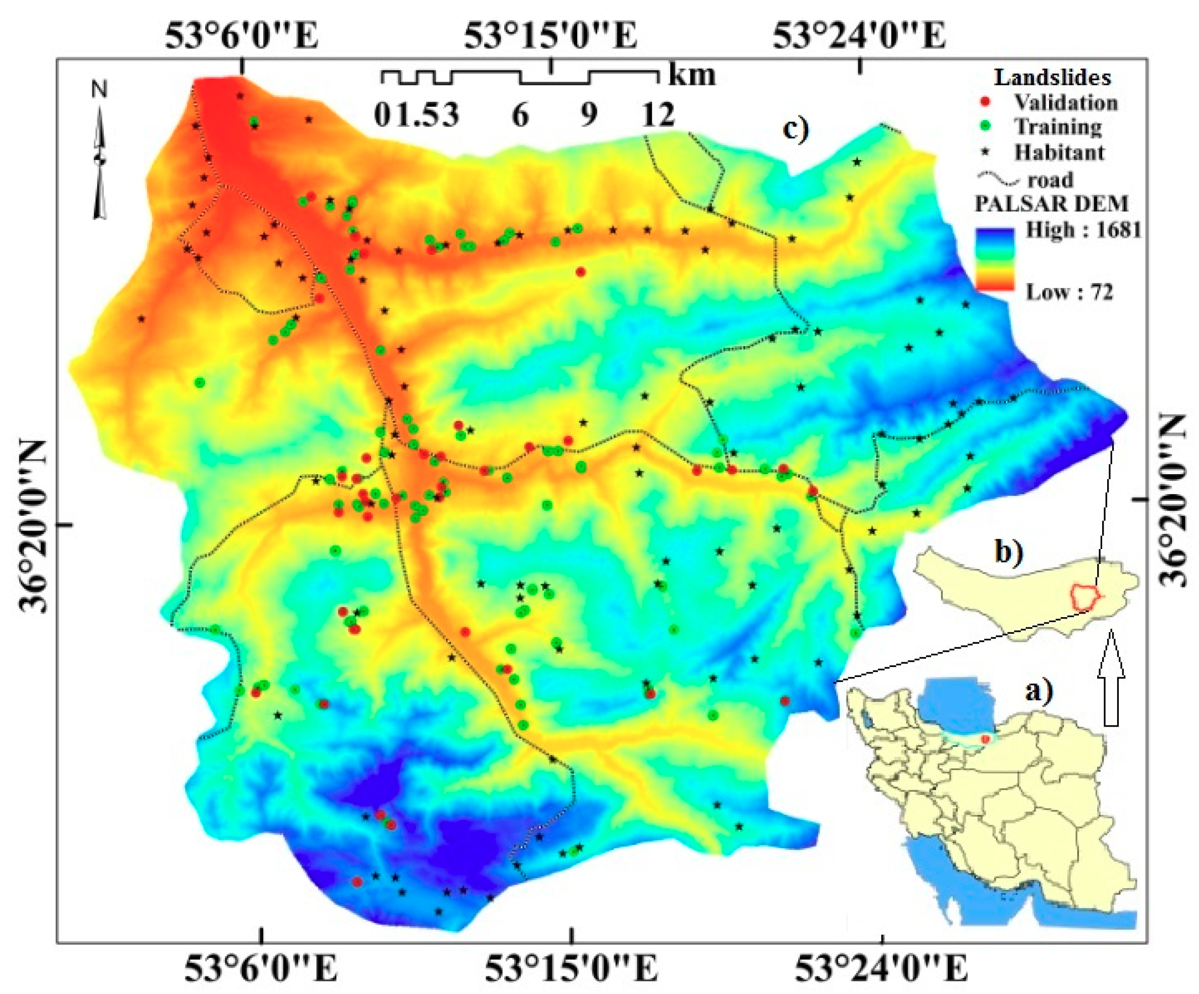
2.1. Study Area

Sangtarashan watershed is located in Mazandran Province, Iran. The area extends to 1072.28 km² and lies between longitudes of 53° 03′ 52″ E and 53° 31′ 39″ E and latitudes of 36° 11′ 48″ N and 36° 30′ 28″ N (Figure 1). The elevation averages 704 m, varying from 72 m in the northeast to 1681 m in the southwest and east of the study area. The mean annual temperature and rainfall are 12.8 °C and 900 mm, respectively [69]. The area is characterised by a mountainous landscape with an average slope gradient of 15.8° and a maximum of 67.8°. The normalised difference vegetation index (NDVI), which varies from −0.132 to 0.639 with a mean of 0.458, indicates a high vegetation density. Convex and concave plan curvature occur on 49.43% and 46.06% of the study area, respectively, whereas only 3.14% has flat topography. The site is characterised by seven land use/land cover (LU/LC) classes, including agricultural lands (0.08%), dense forest (78.9%), low forest (1.5%), agriculture-orchard (7.6%), agricultural forest (0.02%), dry farming forest (11.5%) and water (0.3%). The dominant lithological units in the area [70] are marl, calcareous sandstone, sandy limestone and minor conglomerate (Mm, s, l); hyporite-bearing limestone (K2l1); medium- to thick-bedded limestone (Pel); polymictic conglomerate and sandstone (Plc); and thick-bedded to massive limestone (K2l2).

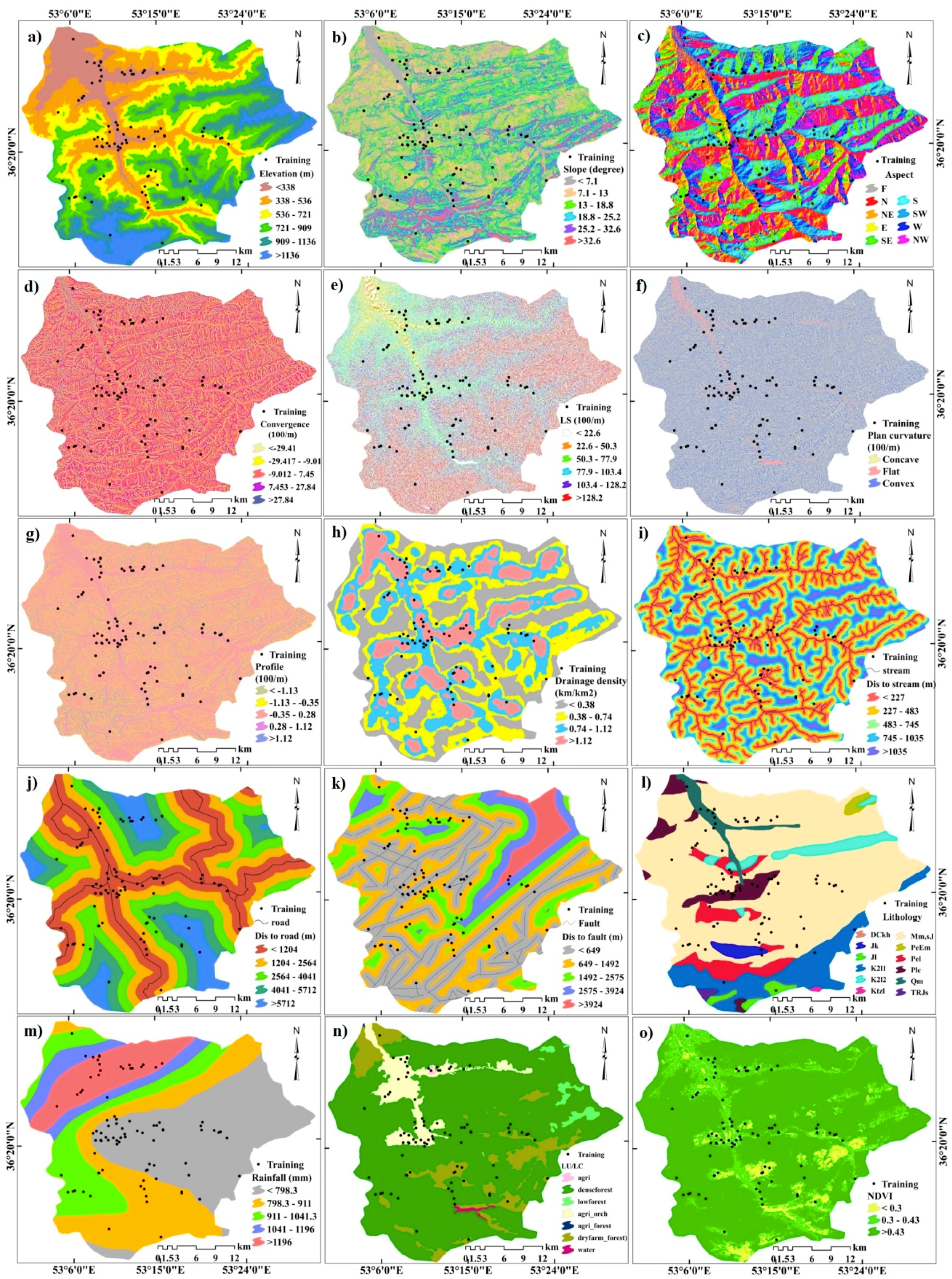
2.2. Data Collection (Landslide Inventory Map and Landslide Conditioning Factors [LCFs])

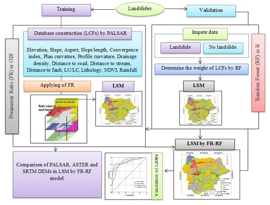
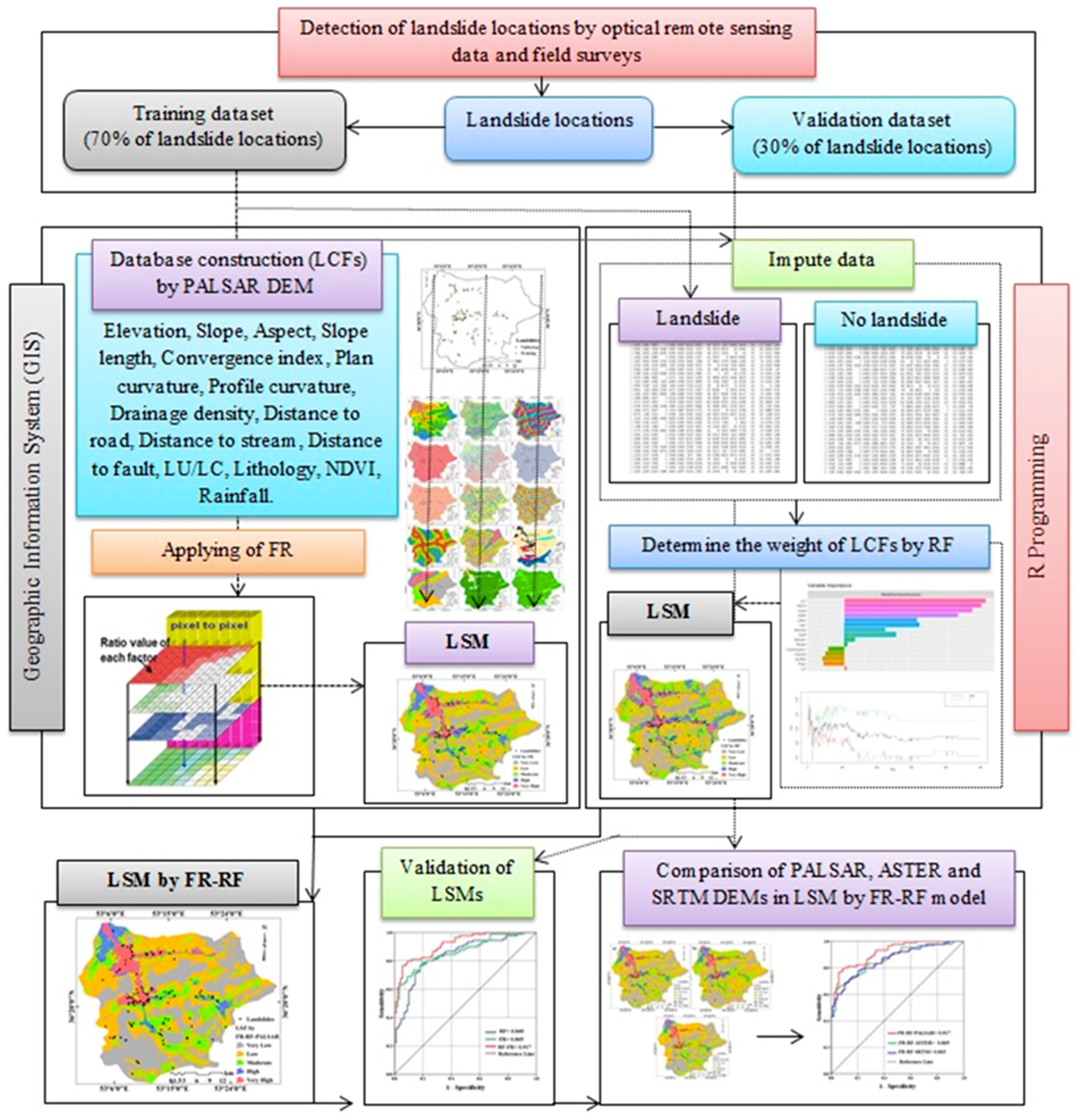
The first step in LS modelling is preparing a landslide inventory. This stage is considered the most important because the accuracy of the landslide inventory used to calibrate the models affects the reliability of LSA [71,72,73]. Thus, the higher the accuracy and quality of the landslide inventory, the better the predictive performance of the susceptibility maps will be [71].

The following are used to produce detailed and reliable landslide inventory map and interpret high-resolution images from Google Earth: (i) Historical landslide records [74]; (ii) interpretation of aerial photos with scales of 1:20,000 and 1:40,000 and high-resolution images available from Google Earth images; and (iii) extensive field surveys in three periods (i.e., 07/12/2016, 06/13/2017 and 03/02/2018). Finally, 129 landslides were identified in the study area from 2013 to 2018. The landslides in the study area are characterised by two modes, that is, slump-tensile and creep-tensile ruptures, which eventually lead to landslide instability. Of these landslides, 70% (90 landslide locations) were selected for training and 30% (39 landslide locations) for validation of the models [12].

Of the 129 landslides identified in the study area, 56 (43.41%) were translational slides, 38 (29.45%) were rotational slides, 5 (3.87%) were soil creep, 23 (17.82%) were shallow translational slide, and 7 (5.42%) were complex slide. These detections covered a total area of 13,324,421 m². Analysis of landslide size showed that the smallest was 135.63 m² and the largest was 976,423 m², with a mean size of 108,215 m². The models developed by [75,76] were used to classify all landslides using landslide points located in the centre of the landslide scar.

On the basis of an extensive literature review [11,40,55,77] and of the physical characteristics of the site, 15 LCFs were used to model the LS in the study area. These LCFs include elevation, slope degree, slope aspect, convergence index, SL, plan curvature, profile curvature, drainage density, distance to stream, distance to road, distance to fault, lithology, rainfall, LU/LC, and NDVI (Figure 2a–o). The variables were submitted to a multicollinearity test that excluded strong relationships among them. The terrain attributes were extracted from PALSAR DEM with 12.5 m spatial resolution (http://www.eorc.jaxa.jp/ALOS/en/aw3d30), DEM-SRTM with 30 m spatial resolution (http://dwtkns.com/srtm30m/), and DEM-ASTER with 90 m spatial resolution (http://dwtkns.com/aster90m/). The slope, aspect, plan curvature, profile curvature, and LS are respectively calculated as follows:

$$\mathrm{Slope}=\sqrt{{\mathrm{H}}^2+{\mathrm{G}}^2}$$

(1)

$$\mathrm{Aspect}=\arctan \left(\frac{\mathrm{H}}{\mathrm{G}}\right)$$

(2)

$$\mathrm{Plan}\mathrm{Curvature}=-\frac{{\mathrm{q}}^2\times \mathrm{r}-2\times \mathrm{p}\times \mathrm{q}\times \mathrm{s}+{\mathrm{p}}^2\times \mathrm{t}}{{\left(\sqrt{1+{\mathrm{P}}^2}+{\mathrm{q}}^2\right)}^3}$$

(3)

$$\mathrm{Profile}\mathrm{Curvature}=-\frac{{\mathrm{q}}^2\times \mathrm{r}+2\times \mathrm{p}\times \mathrm{q}\times \mathrm{r}\times \mathrm{s}+{\mathrm{q}}^2\times \mathrm{t}}{\left({\mathrm{P}}^2+{\mathrm{q}}^2\right)\times {\left(\sqrt{1+{\mathrm{P}}^2}+{\mathrm{q}}^2\right)}^3}$$

(4)

$$LS={\left(\frac{A_S}{22.13}\right)}^{0.6}\times {\left(\frac{Sin\beta }{0.0896}\right)}^{1.3}$$

(5)

where A_s is specific upstream contributing area, and β is the slope gradient. The values of H, G, p, q, r, s and t are obtained as follows:

$$\mathrm{G}=\frac{\mathrm{df}}{\mathrm{dx}}=\frac{\mathrm{Z}3+\mathrm{Z}6+\mathrm{Z}9-\mathrm{Z}1-\mathrm{Z}4-\mathrm{Z}7}{6\times \mathrm{P}}$$

(6)

$$\mathrm{H}=\frac{\mathrm{df}}{\mathrm{dy}}=\frac{\mathrm{Z}1+\mathrm{Z}2+\mathrm{Z}3-\mathrm{Z}4-\mathrm{Z}8-\mathrm{Z}9}{6\times \mathrm{P}}$$

(7)

$$\mathrm{p}=\frac{\mathrm{Z}3+\mathrm{Z}6+\mathrm{Z}9-\mathrm{Z}1-\mathrm{Z}4-\mathrm{Z}7}{6\times {\Delta }_{\mathrm{s}}}$$

(8)

$$\mathrm{q}=\frac{\mathrm{Z}1+\mathrm{Z}2+\mathrm{Z}3-\mathrm{Z}7-\mathrm{Z}8-\mathrm{Z}9}{6\times {\Delta }_{\mathrm{s}}}$$

(9)

$$\mathrm{r}=\frac{\mathrm{Z}1+\mathrm{Z}3+\mathrm{Z}4+\mathrm{Z}6+\mathrm{Z}7+\mathrm{Z}9-2\times \left(\mathrm{Z}2+\mathrm{Z}5+\mathrm{Z}8\right)}{3\times {\Delta }_{\mathrm{s}}^2}$$

(10)

$$\mathrm{s}=\frac{-\mathrm{Z}1+\mathrm{Z}3+\mathrm{Z}7-\mathrm{Z}9}{4\times {\Delta }_{\mathrm{s}}^2}$$

(11)

$$\mathrm{t}=\frac{\mathrm{z}1+\mathrm{z}2+\mathrm{z}3+\mathrm{z}7+\mathrm{z}8+\mathrm{z}9-2\times \left(\mathrm{z}4+\mathrm{z}5+\mathrm{z}6\right)}{3\times {\Delta }_{\mathrm{s}}^2}$$

(12)

where z₁–z₉ are altitude values in 3 × 3 cellular networks and ${\Delta }_s$ denotes the cell size.

The stream network was extracted from the PALSAR DEM using ArcGIS10.5 software to calculate the distance to stream and drainage density. After extracting the stream network, distance to stream and drainage density were calculated using the Euclidean distance and line density tools. To produce the grid of distance to roads, these factors were digitized from 1:50,000 scale topographic maps obtained from the Geographic Organisation of the Armed Forces (2008) and Google Earth satellite images. Next, the distance to road was calculated using the Euclidean distance tool. The same tool was used to extract the grid of distance to faults on the basis of the structural map provided by the Soil Conservation Section of Agricultural and Natural Resources Research Centre of Isfahan Province. The lithological map of the study area, which includes 12 units (

Table 1. Lithology of the study area [70].

Code	Description	Formation	Age
Qm	Swamp and shale	-	Quaternary
Plc	Polymictic conglomerate and sandstone	-	Pliocene
Mm, s, l	Marl, calcareous sandstone, sandy limestone and minor conglomerate	-	Miocene
PeEm	Marl and gypsiferous marl locally gypsiferous mudstone	-	Paleocene–Eocene
K2l2	Thick-bedded to massive limestone	-	Late Cretaceous
K2l1	Hyporite-bearing limestone	-	Late Cretaceous
DCkh	Yellowish, thin to thick-bedded, fossiliferous argillaceous limestone, dark grey limestone, greenish marl and shale, locally including gypsum	-	Devonian
Pel	Medium to thick-bedded limestone	-	Paleocene–Eocene
Jk	Conglomerate, sandstone and shale with plant remains and coal seams	Kashafrud	Middle Jurassic
Jl	Light grey, thin-bedded to massive limestone	Lar	Jurassic–Cretaceous
TRJs	Dark grey shale and sandstone	Shemshad	Triassic–Jurassic
Ktzl	Thick-bedded to massive, white to pinkish orbitolina bearing limestone	Tizkuh	Early Cretaceous

), was prepared on the basis of a 1:100,000 scale geological map [70]. A Landsat 8 image (path 163/ row 35) (7 September 2017), which was archived by USGS with 30 m and 15 m spatial resolution for visual and panchromatic bands, respectively (https://earthexplorer.usgs.gov/), was used to prepare the LU/LC map in ENVI4.8 software. The supervised (maximum likelihood) algorithm was used for this purpose. A set of 375 ground control points were used to validate the LU/LC map with kappa coefficient.

The annual rainfall data recorded at the Talaroum, Afrachal, Soleiman-tangeh, Vasetan, Rigcheshmeh-nakam, Sarkat-tajan and Afrachal weather stations during a 30-year period (i.e., 1986–2016) were interpolated via kriging in ArcGIS10.5 [69] to prepare a rainfall map of the study area. Landsat 8 was used in ArcGIS10.5 software to calculate the NDVI from bands 4 (red band) and 5 (infrared band). The NDVI map was calculated as follows:

NDVI = (IR − R)⁄(IR + R)

(13)

where IR and R represent the infrared and red electromagnetic spectra, respectively.

Table 2. Overview of factors used for landslide susceptibility mapping (LSM).

Factor	Source	Resolution	Classes	Method	Reference
Elevation	PALSAR, ASTER and SRTM DEMs	12.5, 30 and 90 m	(1) <338 m; (2) 338–536 m; (3) 536–721 m; (4) 721–909 m; (5) 909–1136 m; (6) >1136 m	Natural break	[4]
Slope	PALSAR, ASTER and SRTM DEMs	12.5, 30 and 90 m	(1) <7.1°; (2) 7.1°–13°; (3) 13°–18.8°; (4) 18.8°–25.2°; (5) 25.2°–32.6°; (6) >32.6°	Natural break	[78]
Aspect	PALSAR, ASTER and SRTM DEMs	12.5, 30 and 90 m	(1) Flat (−1°); (2) North (337.5°–360°, 0°–22.5°); (3) Northeast (22.5°–67.5°); (4) East (67.5°–112.5°; (5) Southeast (112.5°–157.5°); (6) South (157.5°–202.5°); (7) Southwest (202.5°–247.5°); (8) West (247.4°–292.5°); (9) Northwest (292.5°–337.5°)	Equal interval	[12]
Convergence index	PALSAR, ASTER and SRTM DEMs	12.5, 30 and 90 m	(1) <−29.41); (2) −29.41 to −9.01; (3) −9.01 to 7.45; (4) 7.45–27.84; (5) >27.84	Natural break	[4]
SL	PALSAR, ASTER and SRTM DEMs	12.5, 30 and 90 m	(1) <22.06 m; (2) 22.06–50.3 m; (3) 50.3–77.9 m; (4) 77.9–103.4 m; (5) >103.4 m	Natural break	[79]
Plan curvature	PALSAR, ASTER and SRTM DEMs	12.5, 30 and 90 m	(1) Concave (<0); (2) Flat (0); (3) Convex (>0)	Natural break	[45]
Profile curvature	PALSAR, ASTER and SRTM DEMs	12.5, 30 and 90 m	(1) <−1.13; (2) −1.13 to −0.35; (3) −0.35 to 0.28; (4) 0.28–1.12; (5) >1.12	Natural break	[80]
Drainage density	PALSAR, ASTER and SRTM DEMs	12.5, 30 and 90 m	(1) <0.38 km/km2; (2) 0.38–0.74 km/km2; (3) 0.74–1.12 k m/km2; (4) >1.12 km/km2	Natural break	[60]
Distance to stream	PALSAR, ASTER and SRTM DEMs	12.5, 30 and 90 m	(1) < 227 m; (2) 227–483 m; (3) 483–745 m; (4) 745–1035 m; (5) >1035 m	Natural break	[81]
Distance to road	Topographic map	1:50,000	(1) <1,204 m; (2) 1204–2564 m; (3) 2564–4041 m; (4) 4041–5712 m; (5) >5712 m	Natural break	[45]
Distance to fault	Geological map	1:100,000	(1) <649 m; (2) 649–1492 m; )3) 1492–2575 m; (4) 2575–3924 m; (5) >3924 m	Natural break	[82]
Lithology	Geology map	1:100,000	(1) DCkh; (2) Jk; (3) Jl; (4) K2l1; (5) K2l2; (6) Ktzl; (7) Mm, s, l; (8) PeEm; (9) Pel; (10) Plc; (11) Qm; (12) TRJs	Lithological units	-
Rainfall	Raining data	-	(1) <798.3 mm; (2) 798.3–911 mm; (3) 911–1041.3 mm; (4) 1041–1196 mm; (5) >1196 m m	Natural break	[45]
LU/LC	Landsat-8 image	30 m	(1) Agriculture; (2) Dense forest; (3) Low forest; (4) Agri-orchard; (5) Agri-forest; (6); Dry farming forest; (7) Water	Supervisedclassification	-
NDVI	Landsat-8 image	30 m	(1) <0.3; (2) 0.3–0.43; (3) >0.43	Natural break	[12]

shows the source and resolution of parameters used for classification, along with their classes, methods and references. Finally, all layers were unified similarly with DEM spatial resolution and the UTM Zone39N geographic coordinate system.

2.3. Methodology

The method used in this study (Figure 3) consists of five main steps as follows: (1) Detection of landslide locations by optical remote sensing analysis of Google Earth images and extensive field surveys and random subdivision of the landslide archive into training and validation sets; (2) selection and extraction of 15 LCFs using various data sources, including PALSAR DEM, geological map (1:100,000 scale), topographic map (1:50,000 scale) and Landsat 8 image; (3) application of FR model and establishment of the spatial relationship between LCFs and location of landslides; (4) application of RF model and determination of the importance of LCFs; (5) LSM using two approaches, namely, (i) individual statistical FR and artificial intelligence-based RF models and (ii) FR–RF integrated models; (6) validation of LSMs by calculating AUC parameter; and (7) comparison of FR–RF integrated models prepared using topographic variables extracted from DEMs with different resolutions.

2.4. Models

2.4.1. FR

The FR approach defines a quantitative relationship between landslide occurrence and spatial variability of a set of predictor variables [83]. This method is based on the calculation, for each class of the predictor variables, of the ratio of landslide area within that class to the total landslide area divided by the ratio of the area of that class to the total investigated area. FR is calculated as follows [84]:

$$FR=\frac{\left(\raisebox{1ex}{$A$}\!\left/ \!\raisebox{-1ex}{$B$}\right.\right)}{\left(\raisebox{1ex}{$C$}\!\left/ \!\raisebox{-1ex}{$D$}\right.\right)}=\frac{E}{F}$$

(14)

where A is the number of landslide pixels in each class of the predictors, B is the total number of landslide pixels in the study area, C is the total number of pixels in each class of the predictors, D is the total number of pixels in the study area, E is the percentage of landslide occurrence in each class of the factors, and F is the relative percentage of the area of each subclass of the total area. The FR values of the controlling factors are gathered together in the GIS environment to obtain index of susceptibility to landslide occurrence [85]:

$$LSI={\displaystyle \sum }{\left(FR\right)}_i\left(i=1,2,\dots .,n\right)$$

(15)

where LSI is the landslide susceptibility index, FR is the frequency ratio of factors and n represents the total input factors.

2.4.2. RF

Data mining emerged in the late 1980s, and considerable progress was made in this subject in the 1990s [86]. RF was introduced by [87]. It is a method for the classification and regression of data that combines trees with branches and random data to form an RF. Hence, this method is a collection of regression random trees [88]. Further details about the RF method can be found in [87,89,90,91]. RF analyses have been performed in R 3.3.1 software, using the ‘Randomforest’ package [92].

2.4.3. Ensemble of FR and RF (FR–RF)

Given the shortcomings and limitations of each of the statistical and machine learning models, scientists have proposed and developed integrated methods to overcome their disadvantages and increase their efficiency [93]. In this study, two types of bivariate and machine learning methods, namely, FR and RF, and their ensemble were applied to produce LSM. The FR–RF integrated method eliminates the disadvantages of bivariate methods, such as the failure to calculate the importance of the parameters and disadvantages of machine learning methods, such as the non-calculation of the spatial relationship between the position of the landslides and the parameters that affect them. The main disadvantage of this methodology is the instability of the RF model. A small change in input data leads to a massive change in the tree structure and the output of the model.

2.5. Validation of models

In this experiment, the validation strategy was based on a random partition of the landslide inventory into a calibration set, which includes 70% of landslide locations, and a validation set, which includes 30% of landslide locations [39]. The AUC was used to measure the predictive performance of the models [93,94,95,96,97]. The AUC values, which are in the range of 0–1, was used to classify the accuracy of the landslide predictive models as follows: 0.9–1: excellent accuracy; 0.8–0.9: very good accuracy; 0.7–0.8: good accuracy; 0.6–0.7: moderate accuracy; and 0.5–0.6: poor accuracy [98].

3. Results

3.1. Multicollinearity Test

In LSM, analysing the collinearity among the selected predictors is important as existence of collinearity reduces the performance of the predictive models. Tolerance (TOL) and variance inflation factor (VIF) are commonly used indicators for collinearity between independent variables and were thus used in this study. TOL values less than 0.1 and VIF greater than 10 show collinearity among the predictors [99]. In this study, the values of VIF and TOL were calculated by extracting the values of the parameters in landslide and non-landslide points and analysing them in SPSS16 software. The results of collinearity analysis (

Table 3. Multicollinearity analysis among independent variables.

Model	Unstandardised Coefficients		Standardised Coefficients	t	Sig.	Collinearity Statistics
	B	Std. Error	Beta			Tolerance (TOL)	Variance Inflation Factor (VIF)
(Constant)	1.163	0.483		2.408	0.017
Slope	−0.010	0.009	−0.157	−1.070	0.286	0.154	6.510
Stream power index (SPI)	0.034	0.057	0.125	0.590	0.556	0.074	13.476
Topographic wetness index (TWI)	−0.059	0.052	−0.262	−1.143	0.255	0.063	15.948
LS	0.001	0.001	0.062	1.039	0.300	0.939	1.064
NDVI	−1.063	0.349	−0.220	−3.048	0.003	0.632	1.582
Plan	0.057	0.060	0.082	0.944	0.346	0.442	2.264
Rainfall	0.000	0.000	−0.091	−1.001	0.318	0.401	2.494
Convergence	−0.005	0.002	−0.178	−2.315	0.022	0.558	1.791
Elevation	0.000	0.000	−0.185	−1.611	0.109	0.251	3.980
Dis. to fault	−8.000 × 10−5	0.000	−0.201	−3.201	0.002	0.836	1.197
Dis. to road	−9.013 × 10−6	0.000	−0.036	−0.514	0.608	0.691	1.447
Dis. to stream	0.000	0.000	0.129	1.557	0.121	0.479	2.087
Aspect	−1.151 × 10−5	0.000	−0.002	−0.040	0.968	0.955	1.047
Lithology	0.024	0.045	0.042	0.547	0.585	0.565	1.769
LU/LC	0.059	0.020	0.243	2.985	0.003	0.499	2.003
Profile	−0.0011	0.051	−0.015	−0.215	0.830	0.689	1.452
Drainage	0.217	0.107	0.176	2.020	0.045	0.437	2.286

) indicated that among 17 LCFs, which were initially selected, stream power index (SPI), and topography wetness index (TWI) were highly correlated with TOL (0.063 and 0.074) and VIF (15.94 and 13.47) values exceeding the thresholds. Therefore, SPI and TWI were excluded, and LS modelling in the study area was based on the following variables, which were unaffected by collinearity problems: Elevation, slope degree, slope aspect, convergence index, SL, plan curvature, profile curvature, drainage density, distance to stream, distance to road, distance to fault, lithology, rainfall, LU/LC, and NDVI.

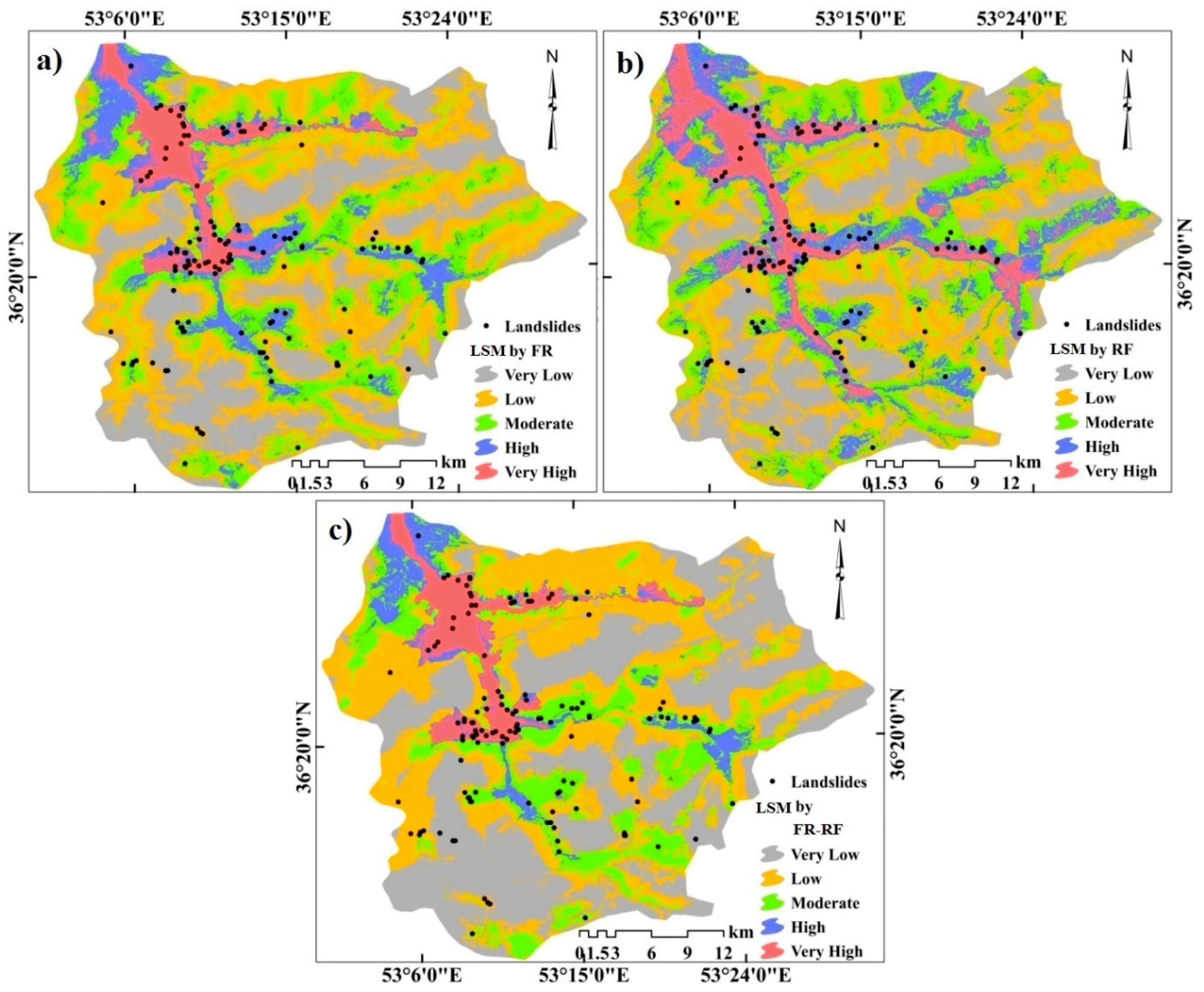
3.2. Application of FR Model

The spatial relationship between the landslides that occurred in the study area and the LCFs are shown in

Table 4. Spatial relationship between conditioning factors and landslide locations with frequency ratio (FR).

Factor	Classes		Pixels in Domain		Landslides		FR
			No.	%	No.	%
Elevation (m)	<338		137,911	11.5753	33	37.0787	3.2032
	338–536		234,710	19.7000	22	24.7191	1.2548
	536–721		259,859	21.8108	21	23.5955	1.0818
	721–909		263,398	22.1079	8	8.9888	0.4066
	909–1136		190,367	15.9781	4	4.4944	0.2813
	>1136		105,177	8.8279	1	1.1236	0.1273
Slope (°)	<7.1		182,669	15.3320	13	14.6067	0.9527
	7.1–13		291,575	24.4729	32	35.9551	1.4692
	13–18.8		278,341	23.3621	23	25.8427	1.1062
	18.8–25.2		219,564	18.4287	11	12.3596	0.6707
	25.2–32.6		153,604	12.8925	5	5.6180	0.4358
	>32.6		65,669	5.5118	5	5.6180	1.0193
Aspect	F		132,288	9.8337	6	6.1856	0.6290
	N		255,671	19.0054	10	10.3093	0.5424
	NE		92,803	6.8986	8	8.2474	1.1955
	E		103,340	7.6818	14	14.4330	1.8788
	SE		123,821	9.2043	9	9.2784	1.0080
	SE		125,536	9.3318	12	12.3711	1.3257
	SW		106,245	7.8978	12	12.3711	1.5664
	W		115,393	8.5778	10	10.3093	1.2019
	NW		136,325	10.1338	8	8.2474	0.8139
Convergence (100/m)	<−29.41		85,228	7.1535	9	10.1124	1.4136
	−29.41 to −9.01		254,471	21.3586	14	15.7303	0.7365
	−9.01 to 7.45		471,169	39.5469	45	50.5618	1.2785
	7.45–27.84		290,876	24.4142	18	20.2247	0.8284
	>27.84		89,675	7.5267	3	3.3708	0.4478
SL (100/m)	<22.06		108,816	18.2882	12	13.4831	0.7373
	22.06–50.3		96,539	16.2249	9	10.1124	0.6233
	50.3–77.9		107,115	18.0023	8	8.9888	0.4993
	77.9–103.4		105,363	17.7079	44	49.4382	2.7919
	103.4–128.2		106,179	17.8450	16	17.9775	1.0074
	>128.2		70,994	11.9316	0	0.0000	0.0000
Plan curvature (100/m)	Concave		564,975	47.4202	41	46.0674	0.9715
	Flat		37,478	3.1457	0	0.0000	0.0000
	Convex		588,969	49.4341	48	53.9326	1.0910
Profile curvature (100/m)	<−1.13		68,989	5.7905	7	7.8652	1.3583
	−1.13 to −0.35		250,549	21.0294	16	17.9775	0.8549
	−0.35 to 0.28		502,333	42.1625	42	47.1910	1.1193
	0.28–1.12		292,982	24.5910	20	22.4719	0.9138
	>1.12		76,569	6.4267	4	4.4944	0.6993
Drainage density (km/km2)	<0.38		330,170	27.7123	5	5.6180	0.2027
	0.38–0.74		365,514	30.6788	18	20.2247	0.6592
	0.74–1.12		320,115	26.8683	37	41.5730	1.5473
	>1.12		175,623	14.7406	29	32.5843	2.2105
Distance to stream (m)		<227	340,196	28.5538	45	50.5618	1.7708
		227–483	304,400	25.5493	22	24.7191	0.9675
		483–745	260,354	21.8524	15	16.8539	0.7713
		745–1035	196,123	16.4613	4	4.4944	0.2730
		>1035	90,349	7.5833	3	3.3708	0.4445
Distance to road (m)		<1204	320,797.2	26.9256	50	56.1798	2.0865
		1204–2564	276,105.2	23.1744	12	13.4831	0.5818
		2564–4041	238,790.2	20.0425	12	13.4831	0.6727
		4041–5712	199,267.2	16.7252	6	6.7416	0.4031
		>5712	1,564,62.2	13.1324	9	10.1124	0.7700
Distance to fault (m)		<649	494,487	41.5039	34	38.2022	0.9204
		649–1492	329,948	27.6936	32	35.9551	1.2983
		1492–2575	196,680	16.5080	19	21.3483	1.2932
		2575–3924	107,320	9.0077	3	3.3708	0.3742
		>3924	62,987	5.2867	1	1.1236	0.2125
Lithology		DCkh	112	0.0094	0	0.0000	0.0000
		Jk	15,756	1.3225	1	1.1236	0.8496
		Jl	14,742	1.2373	1	1.1236	0.9081
		K2l1	135,059	11.3359	3	3.3708	0.2974
		K2l2	45,114	3.7866	0	0.0000	0.0000
		Ktzl	1253	0.1052	0	0.0000	0.0000
		Mm, s, l	803,209	67.4160	61	68.5393	1.0167
		PeEm	9010	0.7562	0	0.0000	0.0000
		Pel	71,877	6.0329	2	2.2472	0.3725
		Plc	56,750	4.7632	15	16.8539	3.5384
		Qm	34,118	2.8636	6	6.7416	2.3542
		TRJs	4422	0.3712	0	0.0000	0.0000
Rainfall (mm)		<798.3	448,287	37.6262	45	50.5618	1.3438
		798.3911	305,254	25.6210	12	13.4831	0.5263
		911–1041.3	195,091	16.3746	9	10.1124	0.6176
		1041–1196	98,934	8.3039	2	2.2472	0.2706
		>1196	143,855	12.0742	21	23.5955	1.9542
LU/LC		Agriculture	976	0.0819	0	0.0000	0.0000
		Dense forest	941,148	78.9937	39	43.8202	0.5547
		Low forest	17,995	1.5104	0	0.0000	0.0000
		Agri-orchard	90,665	7.6098	38	42.6966	5.6107
		Agri-forest	183	0.0154	0	0.0000	0.0000
		Dry farming forest	136,585	11.4640	12	13.4831	1.1761
		Water	3870	0.3248	0	0.0000	0.0000
NDVI		<0.3	116,202	9.7532	26	29.2135	2.9953
		0.3–0.43	177,729	14.9174	29	32.5843	2.1843
		>0.43	897,490	75.3294	34	38.2022	0.5071

. The results showed an inverse relationship between elevation and FR.

The highest value of FR (i.e., 3.2032) was found in the lowest elevation class (<338 m), whereas the lowest value (i.e., 0.1273) was calculated in the highest elevation class (>1136 m). Although a positive relationship between the altitude and FR could be expected for several reasons (e.g., increase of precipitation with elevation), in the study area, low elevation areas exhibited conditions that were more favourable to landslide occurrence due to the presence of deeper soils and higher human pressure at the base of the mountainous areas; this result is consistent with the those of Pourghasemi and Rossi (2016). The highest value of FR (1.4692) was found where the slope angle is low to moderate (7.1°–13°). This result, which is consistent with findings of [72,100], could be related to human activities, such as road construction and LU changes, which are frequently at the base of mountains and may favour slope instability conditions. East (FR = 1.8788) and south-west (FR = 1.5664) slope aspect classes showed a strong correlation with landslide occurrence in the area due to the higher moisture conditions. FR values of convergence index classes (1.4136 and 1.2785) showed higher landslide frequency on classes <−29.41 and −9.01 to 7.45. The FR analysis of the LS factor showed that classes of 77.9–103.4 m with FR = 2.7919 and 103.4–128.2 m with FR = 1.007 had a strong relationship with landslide occurrence in the study area. The analysis of the plan curvature classes showed that the regions with convex and concave topography had a significant effect on landslide occurrence with FR = 1.0910 and 0.9715, respectively. This result was due to the divergence of the flow of water in these slopes and the expansion and contraction of the soil of the convex slopes that had provided conditions favourable for erosion and landslides. These results agree with the findings of [101]. The analysis of profile curvature showed that classes of <−1.13 (FR = 1.3583) and −0.35 to 0.28 (FR = 1.1193) were related to landslides in the study area.

A positive relationship was found between drainage density factor and FR, which showed the highest value (FR = 2.2105) where density of streams was the highest (i.e., >1.12 km⁻¹). As expected, the lowest distance to stream class (<227 m) had a strong relationship with the triggering of landslides, whereas landslides were less frequent as the distance to streams increased. River erosion and saturation at the foot of slopes had a negative effect on the stability and increased the probability of landslide occurrence [102]. The FR analysis of distance to roads showed that areas close to roads had higher susceptibility to landslides. The results of lithology showed that Plc units had a strong relation with landslides and if water penetrates into them, then landslide is more likely to occur. The results of the rainfall parameter showed that the areas that receive the highest amount of rainfall (>1196 mm) with the highest value of FR (1.9542) had the highest potential for landslide occurrence. On the basis of the LU/LC results, a class of agriculture-orchard with FR = 5.6107 had a strong correlation with landslides. These results indicated that human activities could cause the instability of domains and increase landslide occurrence. On the basis of the NDVI factor, the sensitivity of the areas to landslide decreased with the increase in the value of the indicator, indicating the importance of vegetation in reducing mass movements. After determining the weights of the classes of parameters using the FR method, an LSM map was produced using Equation (5) in ArcGIS 10.5 with the weighted sum tool.

$$\begin{array}{l}{\mathrm{LSM}}_{\mathrm{FR}}=\left({\mathrm{W}}_{\mathrm{FR}}\mathrm{Elevation}\right)+\left({\mathrm{W}}_{\mathrm{FR}}\mathrm{Slope}\mathrm{degree}\right)+\left({\mathrm{W}}_{\mathrm{FR}}\mathrm{Slope}\mathrm{aspect}\right)\\ +\left({\mathrm{W}}_{\mathrm{FR}}\mathrm{Convergence}\mathrm{index}\right)+\left({\mathrm{W}}_{\mathrm{FR}}\mathrm{LS}\right)\\ +\left({\mathrm{W}}_{\mathrm{FR}}\mathrm{Plan}\mathrm{curvature}\right)+\left({\mathrm{W}}_{\mathrm{FR}}\mathrm{Profile}\mathrm{curvature}\right)\\ +\left({\mathrm{W}}_{\mathrm{FR}}\mathrm{Drinage}\mathrm{density}\right)+\left({\mathrm{W}}_{\mathrm{FR}}\mathrm{Distance}\mathrm{to}\mathrm{stream}\right)\\ +\left({\mathrm{W}}_{\mathrm{FR}}\mathrm{Distance}\mathrm{to}\mathrm{road}\right)+\left({\mathrm{W}}_{\mathrm{FR}}\mathrm{Distance}\mathrm{to}\mathrm{fault}\right)\\ +\left({\mathrm{W}}_{\mathrm{FR}}\mathrm{Lothology}\right)+\left({\mathrm{W}}_{\mathrm{FR}}\mathrm{Rainfall}\right)+\left({\mathrm{W}}_{\mathrm{FR}}\mathrm{LU}/\mathrm{LC}\right)\\ +\left({\mathrm{W}}_{\mathrm{FR}}\mathrm{NDVI}\right)\end{array}$$

(16)

The resulting LSM obtained using the FR model varied from 6.25 to 17.92. For the classification of the map, four techniques, including equal interval, quantile, natural break and geomatical interval were analysed (Figure 4). Natural break technique was selected due to its high accuracy. Natural break was also used by [103]) as the best classification method for numerical variables. The resulting map was divided into five classes as follows (Figure 5a): Very low (6.25–11.45), low (11.45–14.01), moderate (14.01–17.14), high (17.14–21.77), and very high (21.77–30.39). The results (Figure 4c) showed that 27.11, 33.92, 22.60, 10.24 and 6.11% of the study area were in very low to very high LS classes, respectively.

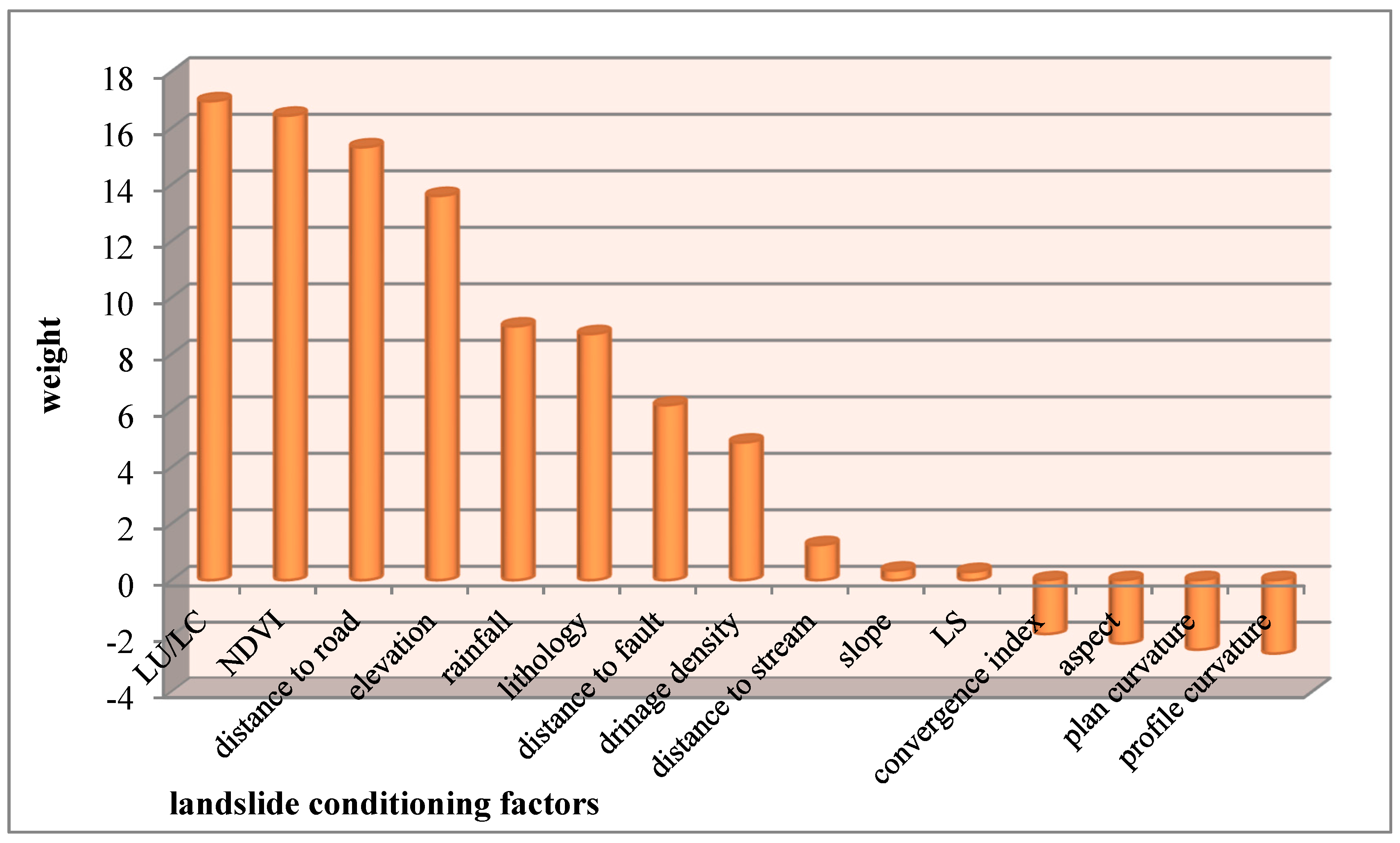
3.3. Application of RF Model

The out-of-bag value of the RF model was 21.6%, and the accuracy of the model was 78.4%. According to the results of the confusion matrix shown in

Table 5. Confusion matrix from random forest (RF) model (0 = non-landslide or negative, 1 = landslide or positive).

Observed	Predicted
	0	1
0	54	10
1	17	44

, out of the 64 non-landslide locations observed, 54 (84.37%) were predicted as non-landslide and 10 (15.62%) as landslide, and out of the 61 observed landslide locations, 17 (27.86%) were predicted as non-landslide and 44 (72.13%) as landslide. The analysis of the importance of LCFs (Figure 6) showed the following ranking: LU/LC (16.95), NDVI (16.44), distance to roads (15.32), elevation (13.6), rainfall (8.98), lithology (8.71), distance to fault (6.19), drainage density (4.87), distance to stream (1.24), slope (0.34), SL (0.29), convergence index (−1.93), aspect (−2.27), plan curvature (−2.49) and profile curvature (−2.63).

The LSM created using the RF model (Figure 5b) was classified according to the natural break method into five classes (very low, low, moderate, high and very high). Approximately 29.23% of the study area is located in low susceptibility class, whereas 8.15% is located in very high susceptibility class (Figure 4c). Approximately 24.26%, 23.51% and 14.83% are located in very low, moderate and high susceptibility classes, respectively.

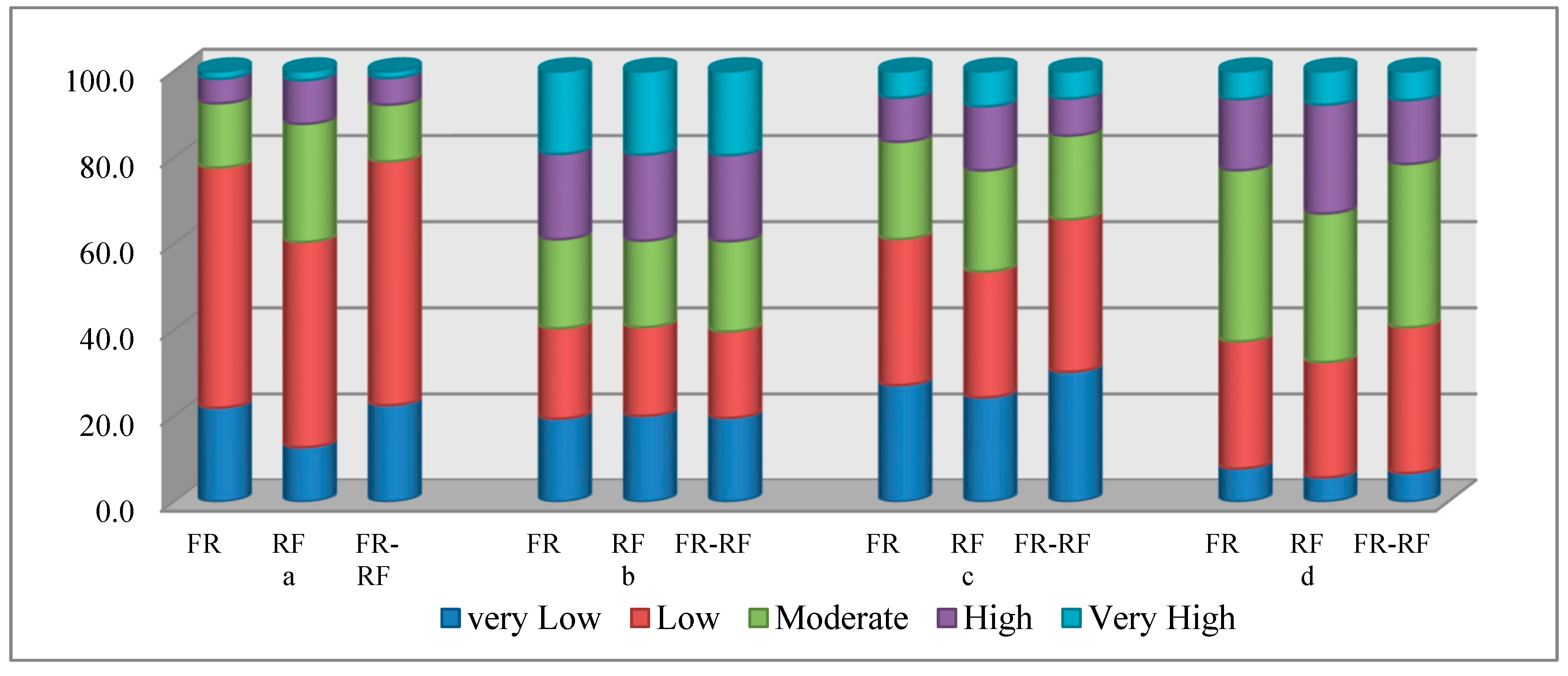
3.4. Application of FR–RF Integrated Model

To calculate LS in the study area by using the FR–RF integrated approach, the following equation was used in ArcGIS10.5 environment:

$$\begin{array}{l}{\mathrm{LSM}}_{\mathrm{FR}-\mathrm{RF}}=\left({\mathrm{W}}_{\mathrm{FR}}\mathrm{Elevation}\times 13.6\right)+\left({\mathrm{W}}_{\mathrm{FR}}\mathrm{Slope}\mathrm{degree}\times 0.34\right)\\ +\left({\mathrm{W}}_{\mathrm{FR}}\mathrm{Slope}\mathrm{aspect}\times -2.27\right)\\ +\left({\mathrm{W}}_{\mathrm{FR}}\mathrm{Convergence}\mathrm{index}\times -1.93\right)+\left({\mathrm{W}}_{\mathrm{FR}}\mathrm{LS}\times 0.29\right)\\ +\left({\mathrm{W}}_{\mathrm{FR}}\mathrm{Plan}\mathrm{curvature}\times -2.49\right)\\ +\left({\mathrm{W}}_{\mathrm{FR}}\mathrm{Profile}\mathrm{curvature}\times -2.63\right)\\ +\left({\mathrm{W}}_{\mathrm{FR}}\mathrm{Drinage}\mathrm{density}\times 4.87\right)\\ +\left({\mathrm{W}}_{\mathrm{FR}}\mathrm{Distance}\mathrm{to}\mathrm{stream}\times 1.24\right)\\ +\left({\mathrm{W}}_{\mathrm{FR}}\mathrm{Distance}\mathrm{to}\mathrm{road}\times 15.32\right)\\ +\left({\mathrm{W}}_{\mathrm{FR}}\mathrm{Distance}\mathrm{to}\mathrm{fault}\times 6.19\right)+\left({\mathrm{W}}_{\mathrm{FR}}\mathrm{Lothology}\times 8.71\right)\\ +\left({\mathrm{W}}_{\mathrm{FR}}\mathrm{Rainfall}\times 8.98\right)+\left({\mathrm{W}}_{\mathrm{FR}}\mathrm{LU}/\mathrm{LC}\times 16.95\right)\\ +\left({\mathrm{W}}_{\mathrm{FR}}\mathrm{NDVI}\times 16.44\right)\end{array}$$

(17)

LS values of the resulting map varied from 19.96 to 278.21. Susceptibility was classified according to natural break method into five classes (Figure 5c), which included 19.96–60.47 (very low), 60.47–88.83 (low), 88.83–127.31 (moderate), 127.31–187.06 (high) and 187.06–278.21 (very high). The results (Figure 4c) indicated that the largest fraction (35.37%) of the study area had low susceptibility, whereas the very high susceptibility class had the smallest extent (6.31%). Very low, moderate, and high susceptibility classes cover 30.23, 19.45, and 8.61% of the study area, respectively.

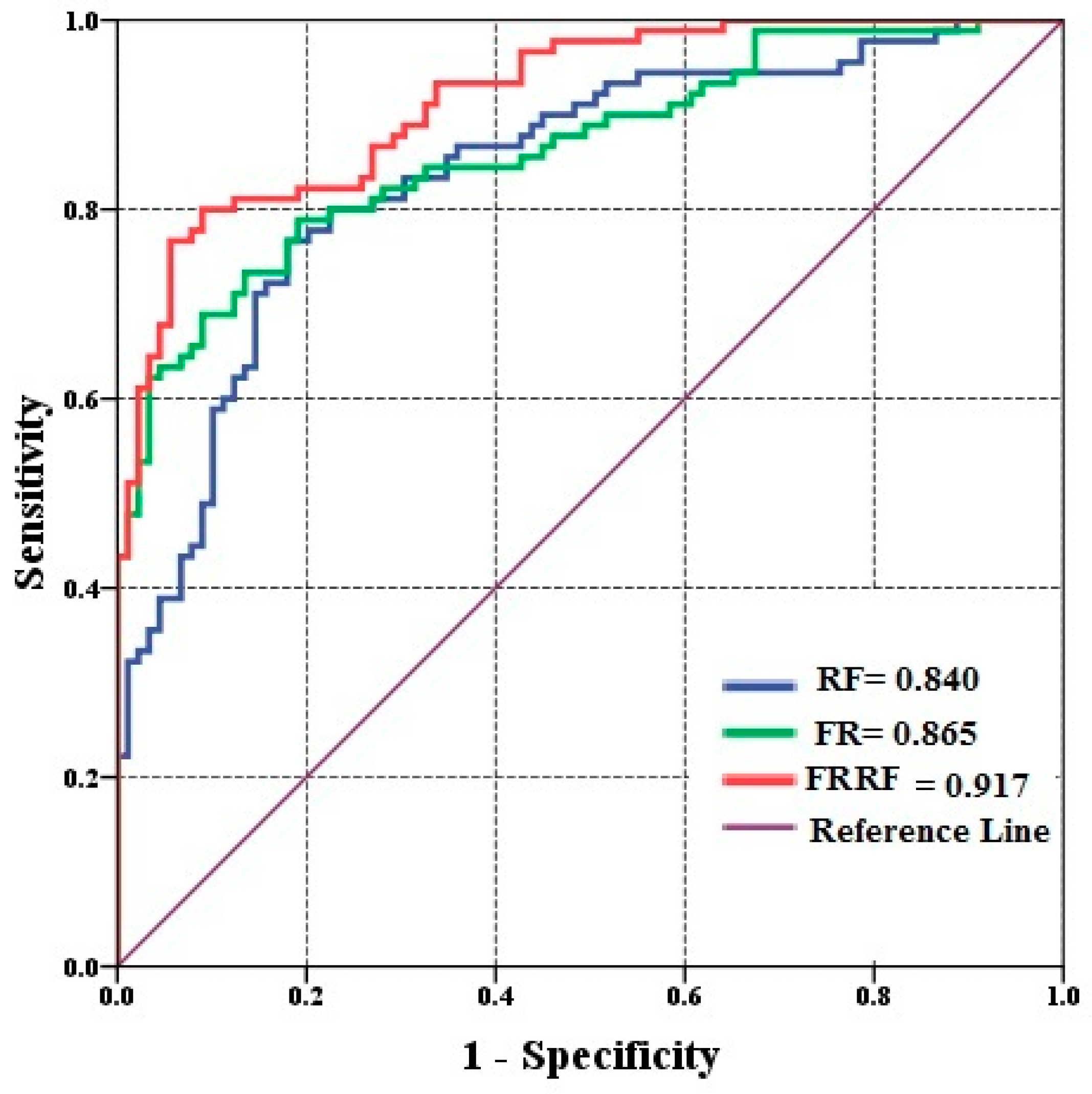
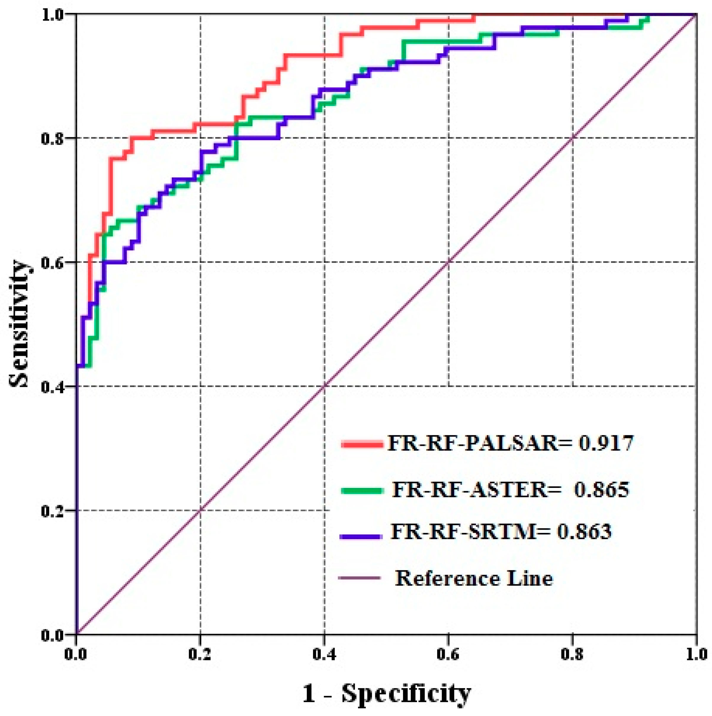
3.5. Model Validation

The results of the model validation using the ROC curve (Figure 7) showed that the FR–RF integrated model (AUC = 0.917) had a higher predictive accuracy compared with the individual methods FR (AUC = 0.865) and RF (AUC = 0.840). To investigate the effect of the resolution of different DEMs on the accuracy of the models, the DEM used in this study (ALOS PALSAR, with 12.5 m spatial resolution) was compared with ASTER and SRTM DEMs with 30 m and 90m spatial resolutions, respectively. The results of comparing the LSM derived from ASTER (Figure 8a) and SRTM (Figure 8b) DEMs and the FR–RF integrated model with the LSM derived from PALSAR DEM and FR–RF integrated model (Figure 5c) showed that the PALSAR DEM provided higher accuracy of the combined approach compared with the other DEMs. The AUC of FR–RF–PALSAR was 0.917, whereas those of FR–RF–ASTER and FR–RF–SRTM approaches were 0.865 and 0.863, respectively (Figure 9).

4. Discussion

In this study, low-frequency radar data (i.e., ALOS PALSAR) was used in providing a DEM to obtain high-precision and high-quality data. The integration of two highly efficient models, namely, FR and RF, was tested to predict areas that are susceptible to landslides accurately. Analysing the varied and complex data related to landslide occurrence requires robust and flexible analytical methods that control nonlinear relationships, interactions, and lost data. Understanding and presenting the results achieved by these methods should be simple and easily interpretable. RF is a powerful and useful data mining technique, which is used for classification and prediction [89]. Tree-based methods can be easily understood by everyone. These methods combine data analysis and modelling; thus, they are a powerful step in modelling. Given its high degree of classification accuracy, the RF has introduced a new method for determining the importance of variables, that is, the capability to model complex interactions between predictor variables and the flexibility to implement different types of statistical data analysis. This method is also useful when complex interactions exist between predictor and response variables and when coherence exists among predictor variables. Another advantage of this method is that it does not need to normalise the data and it can handle nonlinear relationships. The most important disadvantage of this method in the prediction of landslide is the lack of calculation of the spatial relationship between the occurrence of landslides and their effective parameters. Therefore, this method cannot calculate the importance of the classes of each of the parameters in the occurrence of landslide. This problem can be resolved using the FR model. By contrast, the most important disadvantage of the FR model is its incapability to calculate the importance of LCFs, which can be solved using the RF model.

The results of determining the importance of parameters by the RF method showed that parameters LU/LC, NDVI, distance to roads and elevation had the greatest effect on landslide occurrence. These results are in line with the findings of [72,100]. In the results of the model validation, several cases can be mentioned.

(i) The RF model had a higher predictive accuracy compared with the FR model, which is consistent with the results of [18,45,50,57,100]. Chen et al. (2017), Zhang et al. (2016), Kim et al. (2018), and Taaleb et al. (2018). [45]) used the logistic model tree, RF, and classification and regression tree (CART) to prepare an LSM. They used 12 controlling parameters and 171 landslide locations. Their results showed that the RF model had a higher predictive accuracy than the other models. [18] evaluated the LS in China using RF and decision tree models along with GIS techniques. They used 34 hydrological, topographic, geological, LC, and environmental LCFs and 300 landslide locations. They concluded that the RF model had a higher efficiency in identifying sensitive areas to landslide. [50] prepared an LS map at Pyeong-Chang, Korea using RF and boosted tree methods. They used various information layers and divided the landslides that occurred in the area into two groups for modelling (50%) and validation (50%) purposes. Both models had an acceptable accuracy in identifying landslide sensitive areas. [100] evaluated and compared four methods, namely, RF, BRT, CART, and the general linear model (GLM) in LSM in Wadi Tayyah Basin area. The authors used 11 LCFs and 125 landslide locations. The validation of the models, which was performed using success and prediction rate curves, showed that the RF model had a reasonable accuracy in predicting LS and could thus be used to this aim by environmental planners.

(ii) In the experiment, the integration of the individual models (i.e., FR and RF) increased their efficiency. This result is in line with the findings of [32,48,52,56,68]. Ref. [56] combined RF and EBF methods to assess LS. They used 153 landslide locations and 11 effective parameters, namely, slope angle, altitude, TWI, distance from roads, plan curvature, slope aspect, profile curvature, lithology, LU, distance from rivers, and distance to faults. Their results indicated that the integration approach had a higher efficiency in identifying areas susceptible to landslides and eliminate the disadvantages of each individual models.

(iii) The PALSAR DEM had a greater influence on the prediction accuracy of the proposed integrated model compared with ASTER and SRTM DEMs. Moreover, different DEMs derived from various data sources with different spatial resolutions could considerably affect the models’ accuracy. This result is in line with the findings of [104,105], which highlighted that the accuracy of landslide prediction depends on the accuracy and quality of the controlling factors, which in turn depend on the accuracy of their resources, such as DEMs. The methodological framework introduced in this study showed that the integration of models could eliminate their disadvantages and increase their efficiency. Furthermore, the use of radar remote sensing data in comparison with optical data could play a significant role in increasing the prediction accuracy of the models. Thus, using this methodology is recommended in areas with the same environmental conditions.

5. Conclusions

LSM is the first and most important step in managing mountainous areas and reducing the damage caused by landslides. In recent years, many quantitative and qualitative methods have been introduced for LSM. Thus far, no method is considered the best; nevertheless, each one has its obvious advantages and disadvantages. In this study, two statistical- and artificial intelligence-based methods, namely FR and RF, and their integration were used for LSM to promote their advantages and overcome their shortcomings. For this purpose, 15 LCFs (i.e., elevation, slope, slope aspect, convergence index, SL, plan curvature, profile curvature, drainage density, distance to stream, distance to road, distance to fault, lithology, rainfall, LU/LC, and NDVI) and a modelling dataset were used for LSM. The results of RF showed that the LU/LC parameter had the most important role in landslide occurrence in the study area. Validation results showed that the FR–RF integrated model had a higher prediction accuracy than individual models. The results also showed that the quality and accuracy of the input DEMs considerably influenced the prediction accuracy of the resulting LSMs; thus, the resulting LSM from the PALSAR DEM had a higher accuracy compared with the LSM from ASTER and SRTM DEMs. On the basis of the results of the introduced methodology (i.e., FR–RF–PALSAR), 14.92% of the study area is located in high and very high susceptibility classes. The proposed methodology had many advantages (Section 4). The main advantage of this methodology is its capability to determine the relative importance of effective factors and the spatial relationship between these factors and landslide locations. Areas with high sensitivity to landslides are located around residential areas and human infrastructure; thus, any construction in these areas should be performed with caution and observance of engineering principles. The results of this study can be used for LU management, reduction of landslide damages and sustainable development.

References

1. Chen, W.; Li, W.; Hou, E.; Bai, H.; Chai, H.; Wang, D.; Wang, Q. Application of frequency ratio, statistical index, and index of entropy models and their comparison in landslide susceptibility mapping for the Baozhong Region of Baoji, China. Arabian J. Geosci. 2015, 8, 1829–1841. [Google Scholar] [CrossRef]
2. Blöchl, A.; Braun, B. Economic assessment of landslide risks in the Swabian Alb, Germany –research framework and first results of homeowners and experts surveys. Nat. Hazard. Earth Syst. Sci. 2005, 5, 389–396. [Google Scholar] [CrossRef]
3. Komakpanah, A.; Hafezi Moghadas, S. Method of landslide hazard zonation. In Proceedings of the first workshop examined strategies to reduce landslide losses in the country, Tehran, Iran, 1995. [Google Scholar]
4. Arabameri, A.R.; Pourghasemi, H.R.; Yamani, M. Applying different scenarios for landslide spatial modeling using computational intelligence methods. Environ. Earth Sci. 2017, 76, 832. [Google Scholar] [CrossRef]
5. Cruden, D.M. A simple definition of a landslide. Bulletin Int. Assoc. Eng. Geol. 1991, 43, 27–29. [Google Scholar] [CrossRef]
6. Cruden, D.M.; Varnes, D.J. Landslide types and processes. In Landslides, Investigation and Mitigation; Turner, A.K., Schuster, R.L., Eds.; Transportation Research Board: Washington, DC, USA, 1996; pp. 36–75. ISSN 0360–859X. ISBN 030906208X. [Google Scholar]
7. Feizizadeh, B.; Blaschke, T. Landslide risk assessment based on GIS multi-criteria evaluation: A case study in Bostan-Abad County, Iran. J. Earth Sci. Eng. 2011, 1, 66–71. [Google Scholar]
8. Akgun, A.; Kıncal, C.; Pradhan, B. Application of remote sensing data and GIS for landslide risk assessment as an environmental threat to Izmir city (west Turkey). Environ. Monit. Ass. 2012, 184, 5453–5470. [Google Scholar] [CrossRef] [PubMed]
9. Pradhan, B. Landslide hazard and risk analyses at a landslide prone catchment area using statistical based geospatial model. Int. J. Remote Sens. 2011, 32, 4075–4087. [Google Scholar] [CrossRef]
10. Fell, R.; Hartford, D. Landslide risk management. In Proceedings of the international workshop on landslide risk assessment, Honolulu, HI, USA, 19–21 February 1997; pp. 51–109. [Google Scholar]
11. Kavzoglu, T.; Sahin, E.K.; Colkesen, I. Landslide susceptibility mapping using GIS-based multi-criteria decision analysis, support vector machines, and logistic regression. Landslides 2014, 11, 425–439. [Google Scholar] [CrossRef]
12. Arabameri, A.; Pradhan, B.; Rezaei, K.; Sohrabi, M.; Kalantari, Z. GIS-based landslide susceptibility mapping using numerical risk factor bivariate model and its ensemble with linear multivariate regression and boosted regression tree algorithms. J. Mt. Sci 2019, 16, 595–618. [Google Scholar] [CrossRef]
13. Brabb, E.E. Innovative approaches to landslide hazard mapping. In Proceedings of the 4th International Symposium on Landslides, Toronto, Japan, 4 October 1984; pp. 307–324. [Google Scholar]
14. Guzzetti, F.; Reichenbach, P.; Ardizzone, F.; Cardinali, M.; Galli, M. Estimating the quality of landslide susceptibility models. Geomorphology 2006, 81, 166–184. [Google Scholar] [CrossRef]
15. Varnes, D.J. IAEG Commission on Landslides and Other Mass-Movements Landslide Hazard Zonation: A Review of Principles and Practice; UNESCO Press: Paris, France, 1984; Available online: https://www.scirp.org/(S(i43dyn45teexjx455qlt3d2q))/reference/ReferencesPapers.aspx?ReferenceID=1768332 (accessed on 25 April 2019).
16. Wang, L.j.; Kazuhide, S.; Shuji, M. Landslide susceptibility analysis with logistic regression model based On FCM sampling strategy. Comput. Geosci. 2013, 57, 81–92. [Google Scholar] [CrossRef]
17. Kumar, R.; Anbalagan, R. Landslide susceptibility mapping using analytical hierarchy process (AHP) in Tehri reservoir rim region, Uttarakhand. J. Geol. Soc. India 2016, 87, 271–286. [Google Scholar] [CrossRef]
18. Zhang, G.; Cai, Y.; Zheng, Z.; Zhen, J.; Liu, Y.; Huang, K. Integration of the statistical index method and the analytic hierarchy process technique for the assessment of landslide susceptibility in Huizhou, China. CATENA 2016, 142, 233–244. [Google Scholar] [CrossRef]
19. Shahabi, H.; Khezri, S.; Ahmad, B.B.; Hasim, M. Landslide susceptibility mapping at central Zab basin, Iran: A comparison between analytical hierarchy process, frequency ratio and logistic regression models. CATENA 2014, 155, 55–70. [Google Scholar] [CrossRef]
20. Kumar, R.; Anbalagan, R. Landslide susceptibility zonation in part of Tehri reservoir region using frequency ratio, fuzzy logic and GIS. J. Earth Syst. Sci. 2015, 124, 431–448. [Google Scholar] [CrossRef]
21. Youssef, A.M.; Al-Kathery, M.; Pradhan, B. Landslide susceptibility mapping at Al-Hasher Area, Jizan (Saudi Arabia) using GIS-based frequency ratio and index of entropy models. Geosci. J. 2015, 19, 113–134. [Google Scholar] [CrossRef]
22. Roșian, G.; Csaba, H.; Kinga-Olga, R.; Boțan, C.N.; Gavrilă, I.G. Assessing landslide vulnerability using statistical analysis and the frequency ratio model. Case study: Transylvanian Plain (Romania). Geomorphology 2016, 60, 359–371. [Google Scholar]
23. Razavizadeh, S.; Solaimani, K.; Massironi, M.; Kavian, A. Mapping landslide susceptibility with frequency ratio, statistical index, and weights of evidence models: A case study in northern Iran. Environ. Earth Sci. 2017, 76, 499. [Google Scholar] [CrossRef]
24. Nicu, L.C. Application of analytic hierarchy process, frequency ratio, and statistical index to landslide susceptibility: An approach to endangered cultural heritage. Environ. Earth Sci. 2018, 77, 79. [Google Scholar] [CrossRef]
25. Chandra Pal, S.; Chowdhuri, I. GIS-based spatial prediction of landslide susceptibility using frequency ratio model of Lachung River basin, North Sikkim, India. SN Appl. Sci. 2019, 1, 416. [Google Scholar]
26. Costanzo, D.; Chacón, J.; Conoscenti, C.; Irigaray, C.; Rotigliano, E. Forward logistic regression for earth-flow landslide susceptibility assessment in the Platani river basin (southern Sicily, Italy). Landslides 2014, 11, 639–653. [Google Scholar] [CrossRef]
27. Zhang, T.; Han, L.; Han, J.; Li, X.; Zhang, H.; Wang, H. Assessment of Landslide Susceptibility Using Integrated Ensemble Fractal Dimension with Kernel Logistic Regression Model. Entropy 2019, 21, 218. [Google Scholar] [CrossRef]
28. Tsangaratos, P.; Ilia, I. Comparison of a logistic regression and Naïve Bayes classifier in landslide susceptibility assessments: The influence of models complexity and training dataset size. Catena 2016, 145, 164–179. [Google Scholar] [CrossRef]
29. Cama, M.; Conoscenti, C.; Lombardo, L.; Rotigliano, E. Exploring relationships between grid cell size and accuracy for debris-flow susceptibility models: A test in the Giampilieri catchment (Sicily, Italy). Environ. Earth Sci. 2016, 75, 238. [Google Scholar] [CrossRef]
30. Tsangaratos, P.; Ilia, I.; Hong, H.; Chen, W.; Xu, C. Applying Information Theory and GIS-based quantitative methods to produce landslide susceptibility maps in Nancheng County, China. Landslides 2017, 14, 1091–1111. [Google Scholar] [CrossRef]
31. Pradhan, B.; Abokharima, M.H.; Jebur, M.N.; Tehrany, M.S. Land subsidence susceptibility mapping at Kinta Valley (Malaysia) using the evidential belief function model in GIS. Nat. Hazards 2014, 73, 1019–1042. [Google Scholar] [CrossRef]
32. Du, G.; Zhang, Y.; Iqbal, J. Landslide susceptibility mapping using an integrated model of information value method and logistic regression in the Bailongjiang watershed, Gansu Province, China. J. Mount. Sci. 2017, 14, 249. [Google Scholar] [CrossRef]
33. Borrelli, L.; Ciurleo, M.; Gullà, G. Shallow landslide susceptibility assessment in granitic rocks using GIS-based statistical methods: The contribution of the weathering grade map. Landslides 2018, 15, 1127–1142. [Google Scholar] [CrossRef]
34. Kumar, V.; Singh, K. Effectiveness of Remote Sensing and GIS-Based Landslide Susceptibility Zonation Mapping Using Information Value Method. Sustain. Eng. 2019, 17, 225–234. [Google Scholar]
35. Ma, Z.; Qin, S.; Cao, C.; Lv, J.; Li, G.; Qiao, S.; Hu, X. The Influence of Different Knowledge-Driven Methods on Landslide Susceptibility Mapping: A Case Study in the Changbai Mountain Area, Northeast China. Entropy 2019, 21, 372. [Google Scholar] [CrossRef]
36. Hong, H.; Chen, W.; Xu, C.; Youssef, A.M.; Pradhan, B.; Tien Bui, D. Rainfallinduced landslide susceptibility assessment at the Chongren area (China) using frequency ratio, certainty factor, and index of entropy. Geocarto. Int. 2017, 32, 139–154. [Google Scholar]
37. Akgün, A.; Türk, N. Mapping erosion susceptibility by a multivariate statistical method: A case study from the Ayvalık region, NW Turkey. Comput. Geosci. 2011, 37, 1515–1524. [Google Scholar] [CrossRef]
38. Conoscenti, C.; Ciaccio, M.; Caraballo-Arias, N.A.; Gómez-Gutiérrez, Á.; Rotigliano, E.; Agnesi, V. Assessment of susceptibility to earth-flow landslide using logistic regression and multivariate adaptive regression splines: A case of the Belice River basin (western Sicily, Italy). Geomorphology 2015, 242, 49–64. [Google Scholar] [CrossRef]
39. Constantin, M.; Bednarik, M.; Jurchescu, M.C.; Vlaicu, M. Landslide susceptibility assessment using the bivariate statistical analysis and the index of entropy in the Sibiciu Basin (Romania). Environ. Earth Sci. 2011, 63, 397–406. [Google Scholar] [CrossRef]
40. Chen, W.; Pourghasemi, H.R.; Naghibi, S.A. Prioritization of landslide conditioning factors and its spatial modeling in Shangnan County, China using GIS-based data mining algorithms. Bull. Eng. Geo. Environ. 2018, 77, 611. [Google Scholar] [CrossRef]
41. Murillo-García, F.G.; Alcántara-Ayala, I. Landslide Susceptibility Analysis and Mapping Using Statistical Multivariate Techniques: Pahuatlán, Puebla, Mexico. Available online: https://0-link-springer-com.brum.beds.ac.uk/chapter/10.1007/978–3-319–11053–0_16 (accessed on 26 April 2019).
42. Arnone, E.; Francipane, A.; Noto, L.V.; Scarbaci, A.; La Loggia, G. Strategies investigation in using artificial neural network for landslide susceptibility mapping: Application to a Sicilian catchment. J. Hydroinf. 2014, 16, 502–515. [Google Scholar] [CrossRef]
43. Gelisli, K.; Kaya, T.; Babacan, A.E. Assessing the factor of safety using an artificial neural network: Case studies on landslides in Giresun, Turkey. Environ. Earth Sci. 2015, 73, 8639–8646. [Google Scholar] [CrossRef]
44. Tien Bui, D.; Tuan, T.A.; Klempe, H.; Pradhan, B.; Revhaug, I. Spatial prediction models for shallow landslide hazards: A comparative assessment of the efficacy of support vector machines, artificial neural networks, kernel logistic regression, and logistic model tree. Landslides 2016, 13, 361–378. [Google Scholar] [CrossRef]
45. Chen, W.; Xie, X.; Wang, J.; Pradhan, B.; Hong, H.; Tien Bui, D.; Duan, Z.; Ma, J. A comparative study of logistic model tree, random forest, and classification and regression tree models for spatial prediction of landslide susceptibility. Catena 2017, 151, 147–160. [Google Scholar] [CrossRef]
46. Ren, F.; Wu, X.; Zhang, K.; Niu, R. Application of wavelet analysis and a particle swarm-optimized support vector machine to predict the displacement of the Shuping landslide in the Three Gorges, China. Environ. Earth Sci. 2015, 73, 4791–4804. [Google Scholar] [CrossRef]
47. Tien Bui, D.; Pham, B.T.; Nguyen, Q.P.; Hoang, N.D. Spatial prediction of rainfall-induced shallow landslides using hybrid integration approach of least-squares support vector machines and differential evolution optimization: A case study in Central Vietnam. Int. J. Digit. Earth 2016, 9, 1077–1097. [Google Scholar] [CrossRef]
48. Tien Bui, D.; Tuan, T.A.; Hoang, N.D.; Thanh, N.Q.; Nguyen, D.B.; Van Liem, N.; Pradhan, B. Spatial prediction of rainfall-induced landslides for the Lao Cai area (Vietnam) using a hybrid intelligent approach of least squares support vector machines inference model and artificial bee colony optimization. Landslides 2017, 14, 447–458. [Google Scholar] [CrossRef]
49. Kumar, D.; Thakur, M.; Dubey, C.S.; Shukla, D.P. Landslide susceptibility mapping & prediction using support vector machine for Mandakini River Basin, Garhwal Himalaya, India. Geomorphology 2017, 295, 115–125. [Google Scholar]
50. Kim, J.C.; Lee, S.; Jung, H.S.; Lee, S. Landslide susceptibility mapping using Random Forest and boosted tree models in Pyeong-Chang, Korea. J. Geocarto. Int. 2018, 33, 1000–1015. [Google Scholar] [CrossRef]
51. Tien Bui, D.; Pradhan, B.; Lofman, O.; Revhaug, I.; Dick, O.B. Landslide susceptibility mapping at Hoa Binh province (Vietnam) using an adaptive neurofuzzy inference system and GIS. Comput. Geosci. 2012, 45, 199–211. [Google Scholar] [CrossRef]
52. Dehnavi, A.; Aghdam, I.N.; Pradhan, B.; Morshed, V.M.H. A new hybrid model using step-wise weight assessment ratio analysis (SWARA) technique and adaptive neuro-fuzzy inference system (ANFIS) for regional landslide hazard assessment in Iran. Catena 2015, 135, 122–148. [Google Scholar] [CrossRef]
53. Pradhan, B. A comparative study on the predictive ability of the decision tree, support vector machine and neuro-fuzzy models in landslide susceptibility mapping using GIS. Comput. Geosci. 2013, 51, 350–365. [Google Scholar] [CrossRef]
54. Wang, L.J.; Guo, M.; Sawada, K.; Lin, J.; Zhang, J.A. comparative study of landslide susceptibility maps using logistic regression, frequency ratio, decision tree, weights of evidence and artificial neural network. Geosci. J. 2016, 20, 117–136. [Google Scholar] [CrossRef]
55. Hong, H.; Liu, J.; Bui, D.T.; Pradhan, B.; Acharya, T.D.; Pham, B.T.; Zhu, A.X.; Chen, W.; Ahmad, B.B. Landslide susceptibility mapping using J48 Decision Tree with AdaBoost, Bagging and Rotation Forest ensembles in the Guangchang area (China). Catena 2018, 163, 399–413. [Google Scholar] [CrossRef]
56. Pourghasemi, H.R.; Kerle, N. Random forests and evidential belief function-based landslide susceptibility assessment in Western Mazandaran Province, Iran. Environ. Earth Sci. 2016, 75, 1–17. [Google Scholar] [CrossRef]
57. Taaleb, K.; Cheng, T.; Zhang, Y. Mapping landslide susceptibility and types using Random Forest. Big Earth Data. 2018. [CrossRef]
58. Jordan, M.I.; Mitchell, T.M. Machine learning: trends, perspectives, and prospects. Science 2015, 349, 255–260. [Google Scholar] [CrossRef]
59. Aditian, A.; Kubota, T.; Shinohara, Y. Comparison of GIS-based landslide susceptibility models using frequency ratio, logistic regression, and artificial neural network in a tertiary region of Ambon, Indonesia. Geomorphology 2018, 318, 101–111. [Google Scholar] [CrossRef]
60. Arabameri, A.; Rezaei, K.; Pourghasemi, H.R.; Lee, S.; Yamani, M. GIS-based gully erosion susceptibility mapping: A comparison among three data-driven models and AHP knowledge-based technique. Environ. Earth Sci. 2018, 77, 628. [Google Scholar] [CrossRef]
61. Arabameri, A.; Rezaei, K.; Cerda, A.; Conoscenti, C.; Kalantari, Z. A comparison of statistical methods and multi-criteria decision making to map flood hazard susceptibility in Northern Iran. Sci. Total Environ. 2019, 660, 443–458. [Google Scholar] [CrossRef] [PubMed]
62. Abedini, M.; Tulabi, S. Assessing LNRF, FR, and AHP models in landslide susceptibility mapping index: A comparative study of Nojian watershed in Lorestan province, Iran. Environ. Earth Sci. 2018, 77, 405. [Google Scholar] [CrossRef]
63. Immitzer, M.; Atzberger, C.; Koukal, T. Tree species classification with random forest using very high spatial resolution 8-band WorldView-2 satellite data. Remote Sens. 2012, 4, 2661–2693. [Google Scholar] [CrossRef]
64. Arabameri, A.; Rezaei, K.; Cerda, A.; Lombardo, L.; Rodrigo-Comino, J. GIS-based groundwater potential mapping in Shahroud plain, Iran. A comparison among statistical (bivariate and multivariate), data mining and MCDM approaches. Sci. Total Environ. 2019, 658, 160–177. [Google Scholar] [CrossRef]
65. Arabameri, A.; Pradhan, B.; Rezaei, K. Gully erosion zonation mapping using integrated geographically weighted regression with certainty factor and random forest models in GIS. J. Environ. Manag. 2019, 232, 928–942. [Google Scholar] [CrossRef]
66. Yu, K.; Yao, X.; Qiu, Q.; Liu, J. Landslide spatial prediction based on random forest model. J. Chem. Inf. Model. 2017, 47, 2490–2504. [Google Scholar]
67. Arabameri, A.; Pradhan, B.; Pourghasemi, H.R.; Rezaei, K.; Kerle, N. Spatial Modelling of Gully Erosion Using GIS and R Programing: A Comparison among Three Data Mining Algorithms. Appl. Sci. 2018, 8, 1369. [Google Scholar] [CrossRef]
68. Kornejady, A.; Pourghasemi, H.R.; Afzali, S.F. Presentation of RFFR New Ensemble Model for Landslide Susceptibility Assessment in Iran. Available online: https://0-link-springer-com.brum.beds.ac.uk/chapter/10.1007/978-3-319-77377-3_7 (accessed on 28 April 2019).
69. I.R. of Iran Meteorological Organization (IRIMO). Available online: http://www.mazan daranmet.ir (accessed on 23 October 2018).
70. Geology Survey of Iran (GSI). 1997. Available online: http://www.gsi.ir/Main/Lang_en/ index.html. (accessed on 27 October 2018).
71. Guzzetti, F.; Mondini, A.C.; Cardinali, M.; Fiorucci, F.; Santangelo, M.; Chang, K.T. Landslide inventory maps: new tools for and old problem. Earth Sci. Rev. 2012, 112, 42–66. [Google Scholar] [CrossRef]
72. Regmi, A.D.; Devkota, K.C.; Yoshida, K.; Pradhan, B.; Pourghasemi, H.R.; Kumamoto, T.; Akgun, A. Application of frequency ratio, statistical index, and weights-of-evidence models and their comparison in landslide susceptibility mapping in Central Nepal Himalaya. Arabian J. Geosci. 2014, 7, 725–742. [Google Scholar] [CrossRef]
73. Paliaga, G.; Luino, F.; Turconi, L.; Faccini, F. Inventory of geo-hydrological phenomena in Genova municipality (NW Italy). J. Maps 2018, 15, 28–37. [Google Scholar] [CrossRef]
74. Forestry, Rangeland and Watershed Organization (RWO). List of landslides in the Iran. Study Group on Landslides. Office of Engineering and Design Evaluation. 2013. Available online: http://www.frw.org.ir/02/Fa/default.aspx (accessed on 28 April 2019).
75. Varnes D., J. Slope movements, type and processes. In Landslide analysis and control, Transportation Research Board; Schuster, R.L., Krizek, R.J., Eds.; Special Report 176; National Academy Sciences: Washington, DC, USA, 4 May 1978; pp. 11–33. [Google Scholar]
76. Hungr, O.; Leroueil, S.; Picarelli, L. The Varnes classification of landslide types, an update. Landslides 2014, 11, 167–194. [Google Scholar] [CrossRef]
77. Wang, Q.; Li, W.; Wu, Y.; Pei, Y.; Xie, P. Application of statistical index and index of entropy methods to landslide susceptibility assessment in Gongliu (Xinjiang, China). Environ. Earth Sci. 2016, 75, 599. [Google Scholar] [CrossRef]
78. Wu, Y.; Li, W.; Liu, P. Application of analytic hierarchy process model for landslide susceptibility mapping in the Gangu County, Gansu Province, China. Environ. Earth Sci. 2016, 75, 422. [Google Scholar] [CrossRef]
79. Pourghasemi, H.R.; Moradi, H.R.; Fatemi Aghda, S.M. Landslide susceptibility mapping by binary logistic regression, analytical hierarchy process, and statistical index models and assessment of their performances. Nat. Hazards 2013, 69, 749–779. [Google Scholar] [CrossRef]
80. Wang, Y.T.; Seijmonsbergen, A.C.; Bouten, W.; Chen, Q.T. Using statistical learning algorithms in regional landslide susceptibility zonation with limited landslide field data. J. Mount Sci. 2015, 12, 268–288. [Google Scholar] [CrossRef]
81. Achour, Y.; Boumezbeur, R.A.; Hadji, R.; Chouabbi, A.; Cavaleiro, V.; Bendaoud, E.A. Landslide susceptibility mapping using analytic hierarchy process and information value methods along a highway road section in Constantine. Arab J. Geosci. 2017, 10, 194. [Google Scholar] [CrossRef]
82. Pourghasemi, H.R.; Rossi, M. Landslide susceptibility modeling in a landslide prone area in Mazandarn Province, north of Iran: A comparison between GLM, GAM, MARS, and M-AHP methods. Theor. Appl. Climat. 2016, 130, 1–25. [Google Scholar] [CrossRef]
83. Tay, L.T.; Lateh, H.; Hossain, M.K.; Kamil, A.A. Landslide science for a Safer Geoenvironment. Volume 2: Methods of landslide studies Landslide hazard mapping using a poisson distribution: A case study in Penang Island, Malaysia. In Landslide Science for a Safer Geoenvironment; Springer: Cham Switzerland, 29 April 2014; pp. 521–525. [Google Scholar]
84. Ozdemir, A. GIS-based groundwater spring potential mapping in the Sultan Mountains (Konya, Turkey) using frequency ratio, weights of evidence and logistic regression methods and their comparison. J. Hydr. 2011, 411, 290–308. [Google Scholar] [CrossRef]
85. Lee, S.; Pradhan, B. Landslide hazard mapping at Selangor, Malaysia using frequency ratio and logistic regression models. Landslides 2007, 4, 33–41. [Google Scholar] [CrossRef]
86. Chan, C.; Lewis, B. A basic primer on data mining, Information Systems Management. J. Inf. Syst. Manag. 2002, 19, 56–69. [Google Scholar] [CrossRef]
87. Breiman, L. Random forests. Mach. Learn. 2001, 45, 5–32. [Google Scholar] [CrossRef]
88. Biau, G. Analysis of a random forests model. J. Mach. Learn. Res. 2012, 13, 1063–1095. [Google Scholar]
89. Cutler, D.R.; Edwards, T.C.; Beard, K.H.; Cutler, A.; Hess, K.T. Random Forests for Classification in Ecology. Ecology 2007, 88, 2783–2792. [Google Scholar] [CrossRef] [PubMed]
90. Simpson, G.L.; Birks, H.J.B. Statistical learning in palaeolimnology. In Tracking Environmental Change Using Lake Sediments; Springer: Berlin, Germany, 2012. [Google Scholar]
91. Lee, S.; Kim, J.-C.; Jung, H.S.; Lee, M.J.; Lee, S. Spatial prediction of flood susceptibility using random-forest and boosted-tree models in Seoul metropolitan city, Korea. Geomat. Nat. Hazards Risk 2017, 8, 1185–1203. [Google Scholar] [CrossRef]
92. Liaw, A.; Breiman, W.M. Cutler’s Random Forests for Classification and Regression. Available online: https://www.rdocumentation.org/packages/randomForest (accessed on 1 April 2018).
93. Arabameri, A.; Pradhan, B.; Rezaei, K.; Yamani, M.; Pourghasemi, H.R.; Lombardo, L. Spatial modelling of gully erosion using Evidential Belief Function, Logistic Regression and a new ensemble EBF–LR algorithm. Land Degradation Develop. 2018b, 29, 4035–4049. [Google Scholar] [CrossRef]
94. Arabameri, A.; Pradhan, B.; Rezaei, K.; Saro, L.; Sohrabi, M. An Ensemble Model for Landslide Susceptibility Mapping in a Forested Area. Geocarto Int. 2019. [Google Scholar] [CrossRef]
95. Arabameri, A.; Pradhan, B.; Rezaei, K. Spatial prediction of gully erosion using ALOS PALSAR data and ensemble bivariate and data mining models. Geosci. J. 2019, 1–18. [Google Scholar] [CrossRef]
96. Arabameri, A.; Pourghasemi, H.R. Spatial Modeling of Gully Erosion Using Linear and Quadratic Discriminant Analyses in GIS. In Spatial Modeling in GIS and R for Earth and Environmental Sciences, 1st ed.; Pourghasemi, H.R., Gokceoglu, C., Eds.; Elsevier: Berlin, Germany, 2019. [Google Scholar]
97. Shirani, K.; Pasandi, M.; Arabameri, A. Landslide susceptibility assessment by Dempster–Shafer and Index of Entropy models, Sarkhoun basin, Southwestern Iran. Nat. Hazards 2018, 93, 1379–1418. [Google Scholar] [CrossRef]
98. Yesilnacar, E.; Topal, T. Landslide susceptibility mapping: a comparison of logistic regression and neural networks methods in a medium scale study, Hendek region (Turkey). Eng. Geol. 2005, 79, 251–266. [Google Scholar] [CrossRef]
99. Oh, H.J.; Lee, S.; Hong, M. Landslide Susceptibility Assessment Using Frequency Ratio Technique with Iterative Random Sampling. J. Sensors 2017, 2017, 1–22. [Google Scholar] [CrossRef]
100. Youssef, A.M.; Pourghasemi, H.R.; Pourtaghi, Z.S.; Al-Katheeri, M.M. Landslide susceptibility mapping using random forest, boosted regression tree, classification and regression tree, and general linear models and comparison of their performance at Wadi Tayyah Basin, Asir Region, Saudi Arabia. Landslides 2016, 13, 839–856. [Google Scholar] [CrossRef]
101. Chen, T.; Niu, R.; Jia, X. A comparison of information value and logistic regression models in landslide susceptibility mapping by using GIS. Environ. Earth Sci. 2016, 75, 867. [Google Scholar] [CrossRef]
102. Yalcin, A. GIS-based landslide susceptibility mapping using analytical hierarchy process and bivariate statistics in Ardesen (Turkey): Comparisons of results and confirmations. Catena 2008, 72, 1–12. [Google Scholar] [CrossRef]
103. Calvello, M.; Ciurleo, M. Optimal use of thematic maps for landslide susceptibility assessment by means of statistical analyses: case study of shallow landslides in fine grained soils. In Proceedings of the 12th International Symposium on Landslides, Napoli, Italy, 12–19 June 2016. [Google Scholar]
104. Wechsler, S.P. Uncertainties associated with digital elevation models for hydrologic applications: A review. Hydrol. Earth Syst. Sci. 2007, 11, 1481–1500. [Google Scholar] [CrossRef]
105. Garosia, Y.; Sheklabadia, M.; Pourghasemib, H.R.; Besalatpourc, A.A.; Christian Conoscentid, C.; Van Ooste, K. Comparison of differences in resolution and sources of controlling factors for gully erosion susceptibility mapping. Geoderma 2018, 330, 65–78. [Google Scholar] [CrossRef]
Figure 1. Study area: (a) Location of the study area in Iran; (b) location of the study area in Mazandran Province; (c) location of training and validation landslides in the study area.
Remotesensing 11 00999 g001
Figure 2. Landslide conditioning factors (LCFs): (a) elevation; (b) slope degree; (c) slope aspect; (d) convergence index; (e) slope length (SL); (f) plan curvature; (g) profile curvature; (h) drainage density; (i) distance to stream; (j) distance to road; (k) distance to fault; (l) lithology; (m) rainfall; (n) land use/land cover(LU/LC); (o) normalized difference vegetation index (NDVI).
Remotesensing 11 00999 g002
Figure 3. Methodological flowchart.
Remotesensing 11 00999 g003
Figure 4. Classification of resulting map using FR, random forest (RF) and ensemble model: (a) Equal interval; (b) quantile; (c) natural break; (d) geometrical interval.
Remotesensing 11 00999 g004
Figure 5. LSMs using (a) FR, (b) RF and (c) integrated model.
Remotesensing 11 00999 g005
Figure 6. Determining the importance of LCFs using RF.
Remotesensing 11 00999 g006
Figure 7. Area under curve (AUC) values of FR, RF and integrated model.
Remotesensing 11 00999 g007
Figure 8. LSMs using (a) FR–RF–ASTER approach and (b) FR–RF–SRTM approach.
Remotesensing 11 00999 g008
Figure 9. AUC values of FR–RF–PALSAR, FR–RF–ASTER and FR–RF–SRTM.
Remotesensing 11 00999 g009