A Novel Framework to Harmonise Satellite Data Series for Climate Applications

Abstract

Fundamental and thematic climate data records derived from satellite observations provide unique information for climate monitoring and research. Since any satellite only operates over a relatively short period of time, creating a climate data record also requires the combination of space-borne measurements from a series of several (often similar) satellite sensors. Simply combining calibrated measurements from several sensors can, however, produce an inconsistent climate data record. This is particularly true of older, historic sensors whose behaviour in space was often different from their behaviour during pre-launch calibration and more scientific value can be derived from considering the series of historical and present satellites as a whole. Here, we consider harmonisation as a process that obtains new calibration coefficients for revised sensor calibration models by comparing calibrated measurements over appropriate satellite-to-satellite matchups, such as simultaneous nadir overpasses and which reconciles the calibration of different sensors given their estimated spectral response function differences. We present the concept of a framework that establishes calibration coefficients and their uncertainty and error covariance for an arbitrary number of sensors in a metrologically-rigorous manner. We describe harmonisation and its mathematical formulation as an inverse problem that is extremely challenging when some hundreds of millions of matchups are involved and the errors of fundamental sensor measurements are correlated. We solve the harmonisation problem as marginalised errors in variables regression. The algorithm involves computation of first and second-order partial derivatives using Algorithmic Differentiation. Finally, we present re-calibrated radiances from a series of nine Advanced Very High Resolution Radiometer sensors showing that the new time series has smaller matchup differences compared to the unharmonised case while being consistent with uncertainty statistics.

1. Introduction

Stable and accurate long-term Fundamental Climate Data Records (FCDRs) are indispensable for many aspects of climate research and services. Metrological assessment of historical climate trends and climate variability are feasible, if such FCDRs are harmonised and include quantified uncertainties per datum [1,2,3,4]. Such climate data records are also important for assimilation in a reanalysis, as well as for the calculation of statistics that are needed to assess the state of the Earth’s climate and to analyse climate extremes. Unfortunately, disruption of operational routines (such as change of equipment or operator personnel, change of receiving station or environment, and change of observing practices or procedures including changes in the pre-launch analysis) may lead to misleading artifacts. Such artefacts may affect the results of climate data analyses considerably, in particular the results of climate trend analyses. In-flight or post-flight sensor calibration must take particular care to eliminate such artefacts as far as is feasible.

FCDRs usually comprise basic physical quantities such as top of atmosphere (TOA) radiance marked with geographic location and time. Note that radiance may be expressed as, e.g., radiance, brightness temperature, or reflectance. It needs also to be acknowledged that disciplines such as, e.g., altimetry, gravimetry or magnetometry measure signals of a different nature. For convenience, all such signals are in the following referred to as “radiance” without loss of generality. FCDRs constitute the basis for deriving Climate Data Records (CDRs) that comprise higher-level geophysical quantities obtained from combining and transforming FCDR data, with or without an eventual projection onto some form of global grid [3,4].

This study focuses on the problem of creating a multi-decadal FCDR of Earth radiance measurements from a series of similar satellite sensors, each of which operates over a relatively short period of time. Creating a multi-decadal FCDR therefore requires the combination of measurements from several such sensors. For example, Figure 1 illustrates the timeline of the more recent NOAA and MetOp satellites, which have all been equipped with a similar suite of sensors, in particular the Advanced Very High Resolution Radiometer (AVHRR). The thermal channels of AVHRR are comparable to the thermal channels of the Advanced Along Track Scanning Radiometer (AATSR) onboard the Envisat satellite, which in its domain was state of the art from 2002 to 2012.

In this example, there is a lot of overlap in the lifetimes of individual satellites, and at any instant, since 1992, several satellites have been active, such that there are no gaps over time. Earth radiance data from individually-calibrated sensors may differ more than expected; however, even if they measure the same spectral interval and view the same Earth target area at the same time and under similar viewing angles. Simply combining individually-calibrated radiance measurements from different sensors (even if free from disruptive artefacts) may yield inconsistent and unstable FCDRs that exhibit jumps and changes in trends, in particular when past satellite instruments are involved. Small radiance differences are, however, expected because even similar sensors have different spectral response functions. To produce a harmonised FCDR from a series of similar satellite sensors, the sensor measurement models must be recalibrated simultaneously while respecting mutual spectral response differences [1,2]. Some facets of harmonisation resemble standard sensor bias correction and inter-calibration methodologies [5], but harmonisation implements a higher level of metrological rigour and traceability.

Direct Earth observation measurements are telemetry data consisting of digital count numbers related to the incoming radiance (from Earth, space, and internal calibration targets) and information on the sensor state like the temperature of an internal calibration target or the temperature of the instrument and environment. Measurement equations relate these direct observables (usually all on one side of the equation) to the incoming Earth radiance, which constitutes the measurand (usually on the other side of the equation). In addition to direct observables and the measurand itself, the measurement equation includes sensor calibration parameters, which are representative of the measurement principle and of (qualitatively but quantitatively not well known) systematic instrumental effects. Sensor calibration parameters are determined before launch, but the prelaunch calibration is usually not adequate for the full period from launch into space to the end of the mission. In-flight or post-flight recalibration is often achieved by adjusting sensor calibration parameters in such a way that the measured Earth radiance agrees with some (internal or external) reference. A harmonised FCDR then usually refers to a single designated “best” sensor or a series of harmonised “best” sensors, which provides the reference radiance. Alternatively, by including additional constraints, the harmonisation can be based on equally-treated sensors.

An important prerequisite for harmonising fundamental climate data is the assessment of uncertainties associated with the measurement of direct observables and reference radiance [1,2]. Ideally, the assessment associates each datum with an uncertainty. In practice, Earth observation data are evaluated on the basis of pairwise matchup datasets, each of which consists of measurements conducted by two satellites viewing the “same” Earth target at the “same” time and under similar viewing geometries. Harmonisation requires that the uncertainty associated with the matching is assessed. Ideally, the assessment associates each matchup of radiance (either provided by the reference or computed from the sensor measurement equation) with an uncertainty. Similarly, harmonisation requires information about the expected difference in radiances measured by the two sensors due, e.g., to spectral response differences and their associated uncertainty, as well as due to any mismatch between the viewing conditions of the two sensors. Finally, though we may assume that the errors in measurements of the reference radiance are independent, the assumption that the errors in measurements of the direct observables are independent is not always justified. For instance, direct observables, like digital count numbers taken for space and internal calibration targets, are often averaged over time before being put into the measurement equation. Though such averaging reduces the apparent noise, characteristic error correlation structures are created, which harmonisation must take into account.

The metric of harmonisation is defined by a cost function, which quantifies the total mutual misfit of calibrated radiance computed for pairwise matchups, under prescription of expected matchup radiance differences. Finding the best calibration is mathematically equivalent to minimising the cost function. Harmonisation considers errors and error correlation structures in all quantities involved with the harmonisation process. Generic optimisation techniques that implement this paradigm are referred to as errors-in-variables (EIV) techniques [6]. EIV may be interpreted as a generalisation of orthogonal distance regression (ODR) techniques that takes account of error correlation structures, which standard ODR implementations [7] do not.

The harmonisation of the AVHRR series of sensors considers several hundred million measurements of direct observables and reference radiance. The dimension of error covariance matrices associated with these measurements reaches some 10 million, which is beyond the capacity of standard EIV methods. Hunt et al. [8] and Harris et al. [9] have recently developed an EIV implementation to solve these kind of large and highly covariant optimisation problems. Their EIV implementation considers each measurement as a variable parameter, which is subject to optimisation. The dimension of the search space is equal to the number of measurements, which for AVHRR is several 100 million, plus the number of calibration parameters, which is several 10 s. To reduce the dimension of the search space, we have developed a marginalised EIV (MEIV) technique that is based on and generalises the principles of marginalised linear least squares [10]. Like EIV, the MEIV technique takes account of errors and error correlation structures in all quantities involved with the harmonisation process, but only optimises the sensor calibration parameters. MEIV has been applied to the test cases developed by Harris et al. [9] with similar and consistent results.

This paper puts up the mathematical framework to formulate and solve the harmonisation problem and presents results from our initial applications of the MEIV technique to the harmonisation of the AVHRR series of sensors as shown in Figure 1. Section 2 establishes the MEIV cost function, which is minimised to yield a joint maximum posterior probability estimate of all sensor calibration parameters. This estimate is expressed in terms of posterior expected calibration parameter values and the calibration error covariance matrix. Section 3 presents results obtained from applying the MEIV method to solve the problem of harmonising the AVHRR series of sensors ( 11 $\mathsf{\mu }$$\mathrm{m}$ channel only) with respect to the nominal calibrated AATSR TOA radiance as reference. The results are compared with the nominal AVHRR calibration. Section 4 discusses and concludes this paper.

The nomenclature and notation of quantities like time, radiance, uncertainty and error covariance follows the example of Merchant et al. [3] unless noted otherwise.

2. Materials and Methods

2.1. Review of the Single-Sensor Calibration Problem

Let $\mathit{x}(t)=(x_1(t),\cdots ,x_n(t))$ denote some measurements of direct observables acquired at time t, where each $x_l$ is one of the n direct observables that appear in the sensor measurement equation, such as Earth target counts, calibration target counts and measurements of sensor state. Let further $\mathit{\alpha }$ denote the vector of sensor calibration parameters. Then, the generic measurement equation to calculate calibrated radiance $L(t)$ can be written as

$$L(t)=f(t,\mathit{x},\mathit{\alpha }),$$

(1)

where the measurement function f may (or may not) explicitly depend on time. Now, let $\mathit{L}=(L(t_1),\cdots ,L(t_m))$ denote m reference measurements of radiance L conducted at chronologically ordered instants $\mathit{t}=(t_1,\cdots ,t_m)$, and let the matrix

$$\mathit{M}=\left[\begin{array}{ccccc}L(t_1)& x_1(t_1)& x_2(t_1)& \cdots & x_n(t_1)\\ L(t_2)& x_1(t_2)& x_2(t_2)& \cdots & x_n(t_2)\\ ⋮& ⋮& ⋮& \ddots & ⋮\\ \underset{{\displaystyle \mathit{L}}}{\underbrace{L(t_m)}}& \underset{{\displaystyle {\mathit{X}}_1}}{\underbrace{x_1(t_m)}}& \underset{{\displaystyle {\mathit{X}}_2}}{\underbrace{x_2(t_m)}}& \cdots & \underset{{\displaystyle {\mathit{X}}_n}}{\underbrace{x_n(t_m)}}\end{array}\right]\in {\mathbb{R}}^{m\times (1+n)}$$

(2)

represent the set of chronologically ordered pairwise spatio-temporal matchups between reference measurements of radiance L and measurements of sensor state $\mathit{x}$. Any metrologically sound calibration scheme takes account of the uncertainty of each measurement included with $\mathit{M}$ and, if present, any correlation of measurement errors. Let the measurements in each column of the matrix $\mathit{M}$ be independent from all measurements in all other columns, which usually is a valid approximation, but let the errors of measurements within the same column be possibly correlated. To express the uncertainty in measurement, the column of reference measurements $\mathit{L}(\mathit{t})$ is associated with an error covariance matrix $\mathit{S}(\mathit{L})$. Likewise, each column ${\mathit{X}}_l$ of $\mathit{M}$ is associated with an error covariance matrix $\mathit{S}({\mathit{X}}_l)$. Subsuming these matrices under the symbol $\mathit{S}(\mathit{M})$, the problem of single-sensor calibration is mathematically equivalent to the problem of minimising a cost function

$$J(\mathit{\alpha },\mathit{M},\mathit{S}(\mathit{M}))$$

(3)

that expresses the misfit between reference measurements $L(t_1),\cdots ,L(t_m)$ and corresponding values $f(t_1,\mathit{x}(t_1),\mathit{\alpha }),\cdots ,f(t_m,\mathit{x}(t_m),\mathit{\alpha })$ of the measurement equation. The foremost prerequisite for solving the optimisation problem is an adequate representation of the error covariance associated with the individual columns of the matchup data matrix $\mathit{M}$.

2.2. Representation of Uncertainty in Matchup Datasets

The previous section has reviewed the mathematical formalism to calibrate a single sensor and has introduced the matchup data matrix $\mathit{M}$, which is our way to represent a reference-to-sensor matchup dataset. This section generalises this concept, in order to represent arbitrary sensor-to-sensor matchup datasets.

Let ${\mathit{x}}^i(t)=(x_1^i(t),\cdots ,x_{n^i}^i(t))$ denote some measurements acquired at time t, where each $x_l^i$ is one of the $n^i$ direct observables that appear in the measurement function $f^i(t,{\mathit{x}}^i(t),{\mathit{\alpha }}^i)$ of a sensor i with calibration parameters ${\mathit{\alpha }}^i$. In analogy to Equation (2), let the matrix

$${\mathit{M}}^{ij}=\left[\begin{array}{cccccccc}{x}_1^i(t_1^{ij})& x_2^i(t_1^{ij})& \cdots & x_{n^i}^i(t_1^{ij})& x_1^j(t_1^{ji})& x_2^j(t_1^{ji})& \cdots & x_{n^j}^j(t_1^{ji})\\ x_1^i(t_2^{ij})& x_2^i(t_2^{ij})& \cdots & x_{n^i}^i(t_2^{ij})& x_1^j(t_2^{ji})& x_2^j(t_2^{ji})& \cdots & x_{n^j}^j(t_2^{ji})\\ ⋮& ⋮& \ddots & ⋮& ⋮& ⋮& \ddots & ⋮\\ \underset{{\displaystyle {\mathit{X}}_1^{ij}}}{\underbrace{x_1^i(t_m^{ij})}}& \underset{{\displaystyle {\mathit{X}}_2^{ij}}}{\underbrace{x_2^i(t_m^{ij})}}& \cdots & \underset{{\displaystyle {\mathit{X}}_{n^i}^{ij}}}{\underbrace{x_{n^i}^i(t_m^{ij})}}& \underset{{\displaystyle {\mathit{X}}_1^{ji}}}{\underbrace{x_1^j(t_m^{ji})}}& \underset{{\displaystyle {\mathit{X}}_2^{ji}}}{\underbrace{x_2^j(t_m^{ji})}}& \cdots & \underset{{\displaystyle {\mathit{X}}_{n^j}^{ji}}}{\underbrace{x_{n^j}^j(t_m^{ji})}}\end{array}\right]\in {\mathbb{R}}^{m\times (n^i+n^j)}$$

(4)

represent the set of chronologically ordered pairwise spatio-temporal matchups of telemetry data acquired by the sensor i with telemetry data acquired by another sensor j. The ordered instants ${\mathit{t}}^{ij}=(t_1^{ij},\cdots ,t_m^{ij})$ and ${\mathit{t}}^{ji}=(t_1^{ji},\cdots ,t_m^{ji})$ may differ within a tolerance prescribed by given matchup selection criteria. Note that the reference-to-sensor matchup data matrix defined in Equation (2) is a specialisation of the general sensor-to-sensor matchup data matrix of Equation (4) where the single telemetry datum of sensor i is radiance and the measurement function $f^i$ is the identity function.

Now again, let the measurements in each column of the matchup data matrix ${\mathit{M}}^{ij}$ be independent from all measurements in all other columns, but let the errors of measurements within the same column be possibly correlated. Thus, to describe the uncertainty associated with the matchup dataset represented by ${\mathit{M}}^{ij}$, we may consider any generic column of ${\mathit{M}}^{ij}$ and our generic description will apply to all other columns as well. Therefore, let

$$\mathit{q}=\left[\begin{array}{c}q(t_1)\\ q(t_2)\\ ⋮\\ q(t_m)\end{array}\right]\in {\mathbb{R}}^m$$

(5)

denote any column of ${\mathit{M}}^{ij}$. The description of the error covariance matrix $\mathit{S}(\mathit{q})\in {\mathbb{R}}^{m\times m}$ is straightforward, but there are several cases to discern.

• Independent random errors—arise from uncorrelated, i.e., independent, random error effects. Each measurement included with $\mathit{q}$ exhibits an error that is random and independent from the errors of all other measurements. The error covariance matrix ${\mathit{S}}_{\mathrm{i}}(\mathit{q})$ is diagonal with elements that represent the variance of each error. Let

  $$\mathit{U}(\mathit{q})=\left[\begin{array}{cccc}u(q(t_1))& 0& \cdots & 0\\ 0& u(q(t_2))& \cdots & 0\\ ⋮& ⋮& \ddots & ⋮\\ 0& 0& \cdots & u(q(t_m))\end{array}\right]\in {\mathbb{R}}^{m\times m}$$

  (6)

  define the diagonal uncertainty matrix; thus, the error covariance matrix ${\mathit{S}}_{\mathrm{i}}(\mathit{q})$, which is diagonal and of full rank, is given by

  $${\mathit{S}}_{\mathrm{i}}(\mathit{q})={(\mathit{U}(\mathit{q}))}^2.$$

  (7)
• Common random errors—arise from a fully correlated, i.e., common, random error effect. All measurements in $\mathit{q}$ exhibit an error that is due to the same random effect e. Let $u(e)$ denote the uncertainty associated with this effect and let ${\mathit{C}}_e(\mathit{q})\in {\mathbb{R}}^m$ be the absolute sensitivity of $\mathit{q}$ with respect to e. Then, the law of propagation of uncertainty [11] states that the uncertainty of the measurements $\mathit{q}$ which results from each such effect e is

  $${\mathit{u}}_e(\mathit{q})=u(e){\mathit{C}}_e(\mathit{q})\in {\mathbb{R}}^m$$

  (8)

  and that the error covariance matrix ${\mathit{S}}_e(\mathit{q})$, which is dense and of rank one, is given by

  $${\mathit{S}}_e(\mathit{q})={\mathit{u}}_e(\mathit{q}){({\mathit{u}}_e(\mathit{q}))}^{\mathrm{T}}.$$

  (9)
• Structured random errors—arise when the measurements in $\mathit{q}$ are not original measurements but rather result from an operation on an underlying (and usually larger) set of $m^{\prime }$ original measurements of the same quantity q measured at instants $t_1^{\prime },\cdots ,t_{m^{\prime }}^{\prime }$, i.e.,

  $${\mathit{q}}^{\prime }=\left[\begin{array}{c}q(t_1^{\prime })\\ q(t_2^{\prime })\\ ⋮\\ q(t_{m^{\prime }}^{\prime })\end{array}\right]\in {\mathbb{R}}^{m^{\prime }},$$

  (10)

  and these $m^{\prime }$ measurements have independent random errors (case 1) associated with them. A common example operation would be some form of averaging [1,2], but any linear mapping of measurements from ${\mathit{q}}^{\prime }$ to $\mathit{q}$ is permissible. Let $\mathit{q}=\mathit{W}{\mathit{q}}^{\prime }$, where $\mathit{W}\in {\mathbb{R}}^{m\times m^{\prime }}$ is the matrix that defines the linear operation. Thus, the error covariance matrix ${\mathit{S}}_{\mathrm{s}}(\mathit{q})$, which is typically sparse and of rank $min(m,m^{\prime })$, is given by

  $${\mathit{S}}_{\mathrm{s}}(\mathit{q})=\mathit{W}{(\mathit{U}({\mathit{q}}^{\prime }))}^2{\mathit{W}}^{\mathrm{T}}.$$

  (11)
• Structured common random errors—arise when the measurements in $\mathit{q}$ are not original measurements, but result from an operation on an underlying set of original measurements ${\mathit{q}}^{\prime }$ that have both independent random errors (case 1) and systematic errors (case 2) associated with them. Let

  $$\mathit{q}=\mathit{W}{\mathit{q}}^{\prime }$$

  (12)

  as in the third case. Here, the error covariance matrix is dense and given by

  $$\mathit{S}(\mathit{q})=\mathit{W}\left[{(\mathit{U}({\mathit{q}}^{\prime }))}^2+{\mathit{u}}_e({\mathit{q}}^{\prime }){({\mathit{u}}_e({\mathit{q}}^{\prime }))}^{\mathrm{T}}\right]{\mathit{W}}^{\mathrm{T}},$$

  (13)

  which, because ${\mathit{u}}_e(\mathit{q})=\mathit{W}{\mathit{u}}_e({\mathit{q}}^{\prime })$, is equivalent to

  $$\mathit{S}(\mathit{q})=\mathit{W}{(\mathit{U}({\mathit{q}}^{\prime }))}^2{\mathit{W}}^{\mathrm{T}}+{\mathit{u}}_e(\mathit{q}){({\mathit{u}}_e(\mathit{q}))}^{\mathrm{T}}.$$

  (14)

Equation (14) demonstrates that the fourth case is a simple combination of the second and the third case, and only the first three cases are genuinely different. Indeed, the error covariance matrix $\mathit{S}(\mathit{q})$ may always be expressed by any of the basic Equations (7), (9) and (11) or any combination thereof as, e.g., in Equation (14). Note that knowledge of the sparsity and rank deficiency of the basic matrices is the key to implement storage and computationally efficient matrix representation schemes on a computer.

The error covariance matrix may also be expressed in radiance-equivalent form by propagating the uncertainty associated with each column ${\mathit{X}}_1^{ij}\cdots ,{\mathit{X}}_{n^i}^{ij}$ and each column ${\mathit{X}}_1^{ji}\cdots ,{\mathit{X}}_{n^j}^{ji}$ to the calibrated radiance

$${\mathit{L}}^{ij}({\mathit{\alpha }}^i)=\left[\begin{array}{c}{f}^i(t_1^{ij},{\mathit{x}}^i(t_1^{ij}),{\mathit{\alpha }}^i)\\ f^i(t_2^{ij},{\mathit{x}}^i(t_2^{ij}),{\mathit{\alpha }}^i)\\ ⋮\\ f^i(t_m^{ij},{\mathit{x}}^i(t_m^{ij}),{\mathit{\alpha }}^i)\end{array}\right]\in {\mathbb{R}}^m\mathrm{and}{\mathit{L}}^{ji}({\mathit{\alpha }}^j)=\left[\begin{array}{c}{f}^j(t_1^{ji},{\mathit{x}}^j(t_1^{ji}),{\mathit{\alpha }}^j)\\ f^j(t_2^{ji},{\mathit{x}}^j(t_2^{ji}),{\mathit{\alpha }}^j)\\ ⋮\\ f^j(t_m^{ji},{\mathit{x}}^j(t_m^{ji}),{\mathit{\alpha }}^j)\end{array}\right]\in {\mathbb{R}}^m$$

(15)

of sensors i and j, respectively. Let

$${\mathit{D}}_l^{ij}({\mathit{\alpha }}^i)=\left[\begin{array}{cccc}{\displaystyle \frac{\partial f^i}{\partial x_l^i}}(t_1^{ij},{\mathit{x}}^i(t_1^{ij}),{\mathit{\alpha }}^i)& 0& \cdots & 0\\ 0& {\displaystyle \frac{\partial f^i}{\partial x_l^i}}(t_2^{ij},{\mathit{x}}^i(t_2^{ij}),{\mathit{\alpha }}^i)& \cdots & 0\\ ⋮& ⋮& \ddots & ⋮\\ 0& 0& \cdots & {\displaystyle \frac{\partial f^i}{\partial x_l^i}}(t_m^{ij},{\mathit{x}}^i(t_m^{ij}),{\mathit{\alpha }}^i)\end{array}\right]\in {\mathbb{R}}^{m\times m}$$

(16)

designate the sensitivity (i.e., the Jacobian matrix) of the calibrated radiance ${\mathit{L}}^{ij}$ of sensor i with respect to the column ${\mathit{X}}_l^{ij}$, and let

$${\mathit{D}}_l^{ji}({\mathit{\alpha }}^j)=\left[\begin{array}{cccc}{\displaystyle \frac{\partial f^j}{\partial x_l^j}}(t_1^{ji},{\mathit{x}}^j(t_1^{ji}),{\mathit{\alpha }}^j)& 0& \cdots & 0\\ 0& {\displaystyle \frac{\partial f^j}{\partial x_l^j}}(t_2^{ji},{\mathit{x}}^j(t_2^{ji}),{\mathit{\alpha }}^j)& \cdots & 0\\ ⋮& ⋮& \ddots & ⋮\\ 0& 0& \cdots & {\displaystyle \frac{\partial f^j}{\partial x_l^j}}(t_m^{ji},{\mathit{x}}^j(t_m^{ji}),{\mathit{\alpha }}^j)\end{array}\right]\in {\mathbb{R}}^{m\times m}$$

(17)

correspondingly designate the sensitivity of the calibrated radiance ${\mathit{L}}^{ji}$ of sensor j with respect to the column ${\mathit{X}}_l^{ji}$. Then, the law of propagation of uncertainty [11] states that the radiance error covariance matrices $\mathit{S}({\mathit{L}}^{ij})$ and $\mathit{S}({\mathit{L}}^{ji})$ are given by

$$\begin{array}{cc}\hfill \mathit{S}({\mathit{L}}^{ij}({\mathit{\alpha }}^i))& =\sum _{l=1}^{n^i}{\mathit{D}}_l^{ij}({\mathit{\alpha }}^i)\mathit{S}({\mathit{X}}_l^{ij}){({\mathit{D}}_l^{ij}({\mathit{\alpha }}^i))}^{\mathrm{T}}\hfill \end{array}$$

(18)

and

$$\begin{array}{cc}\hfill \mathit{S}({\mathit{L}}^{ji}({\mathit{\alpha }}^j))& =\sum _{l=1}^{n^j}{\mathit{D}}_l^{ji}({\mathit{\alpha }}^j)\mathit{S}({\mathit{X}}_l^{ji}){({\mathit{D}}_l^{ji}({\mathit{\alpha }}^j))}^{\mathrm{T}}.\hfill \end{array}$$

(19)

To express the error covariance matrix of the differences of calibrated radiance ${\mathit{L}}^{ij}-{\mathit{L}}^{ji},$ we must take account of the fact that any two sensors i and j do not usually observe the same Earth target at the same time and under the same conditions. Let ${\mathit{K}}_{\mathrm{m}}^{ij}$ denote the differences between the calibrated radiances we expect because of these types of matchup differences. In the absence of better knowledge, we may expect ${\mathit{K}}_{\mathrm{m}}^{ij}=0,$ but, even in this case, we must associate an error covariance matrix with this expectation. Let the errors in our expectation ${\mathit{K}}_{\mathrm{m}}^{ij}$ be random and independent, thus

$$\mathit{S}({\mathit{K}}_{\mathrm{m}}^{ij})={(\mathit{U}({\mathit{K}}_{\mathrm{m}}^{ij}))}^2.$$

(20)

In general, even similar sensors i and j will have different spectral response functions and we cannot expect that the differences ${\mathit{L}}^{ij}-{\mathit{L}}^{ji}-{\mathit{K}}_{\mathrm{m}}^{ij}$ will vanish. Let ${\mathit{K}}_{\mathrm{s}}^{ij}$ denote the differences of calibrated radiance we expect because of mutual differences in the two sensors’ spectral response functions. Thus, we may write

$$\mathit{S}({\mathit{K}}_{\mathrm{s}}^{ij})={(\mathit{U}({\mathit{K}}_{\mathrm{s}}^{ij}))}^2,$$

(21)

where we again have assumed that the errors in our expectation ${\mathit{K}}_{\mathrm{s}}^{ij}$ are all independent and random. Finally, we write

$$\mathit{S}({\mathit{d}}^{ij}({\mathit{\alpha }}^i,{\mathit{\alpha }}^j)-{\mathit{K}}^{ij})=\sum _{l=1}^{n^i}{\mathit{D}}_l^{ij}({\mathit{\alpha }}^i)\mathit{S}({\mathit{X}}_l^{ij}){({\mathit{D}}_l^{ij}({\mathit{\alpha }}^i))}^{\mathrm{T}}+\sum _{l=1}^{n^j}{\mathit{D}}_l^{ji}({\mathit{\alpha }}^j)\mathit{S}({\mathit{X}}_l^{ji}){({\mathit{D}}_l^{ji}({\mathit{\alpha }}^j))}^{\mathrm{T}}+\mathit{S}({\mathit{K}}^{ij}),$$

(22)

where

$${\mathit{d}}^{ij}({\mathit{\alpha }}^i,{\mathit{\alpha }}^j)={\mathit{L}}^{ij}({\mathit{\alpha }}^i)-{\mathit{L}}^{ji}({\mathit{\alpha }}^j)$$

(23)

are the differences of calibrated radiance we measure, ${\mathit{K}}^{ij}={\mathit{K}}_{\mathrm{m}}^{ij}+{\mathit{K}}_{\mathrm{s}}^{ij}$ are the differences of calibrated radiance we expect because of matchup and spectral response differences in total, and

$$\mathit{S}({\mathit{K}}^{ij})={(\mathit{U}({\mathit{K}}_{\mathrm{m}}^{ij}))}^2+{(\mathit{U}({\mathit{K}}_{\mathrm{s}}^{ij}))}^2.$$

(24)

In the remainder of this paper, we refer to the double differences ${\mathit{d}}^{ij}({\mathit{\alpha }}^i,{\mathit{\alpha }}^j)-{\mathit{K}}^{ij}$ as K-residuals. For a perfect harmonisation, the mean K residual will be zero.

2.3. Formulation of the Harmonisation Problem

Harmonisation describes the joint calibration of a series of sensors that are all manufactured to make the same measurement, e.g., Earth radiance in a particular spectral band. To formulate the harmonisation problem in a generic way, let the sensors in our series be enumerated by i and j such that $i=1$ designates the reference sensor and the matchup data matrix ${\mathit{M}}^{ij}$ with $i\ge 1$ and $j>i$ represents the pairwise spatio-temporal matchups between two sensors i and j as in Equation (4). Let all sensor calibration parameters be subsumed under the symbol $\mathit{\alpha }$ and let all reference radiance and sensor telemetry data be subsumed under the symbol $\mathit{X}$. Furthermore, let $\check{\mathit{\alpha }}$ denote any a priori expected values of $\mathit{\alpha }$ and let $\mathit{S}(\widehat{\mathit{\alpha }})$ denote the a priori associated error covariance matrix.

2.3.1. EIV Formulation

The EIV technique considers all measurements $\mathit{X}$ as variable parameters, in order to take all measurement errors and error correlation structures into account, such as the sensor calibration parameters $\mathit{\alpha }$. To distinguish (in this subsection only) between variable parameters and invariant measurements thereof, let $\check{\mathit{X}}$ denote the measurements and let $\mathit{X}$ denote the variables. In a Bayesian context and in analogy to $\check{\mathit{\alpha }}$ and $\mathit{S}(\check{\mathit{\alpha }})$, the measurements $\check{\mathit{X}}$ designate the a priori expected values of the parameters $\mathit{X}$ while $\mathit{S}(\check{\mathit{X}})$ embodies the a priori associated error covariance matrix. Hence, the harmonisation problem is equivalent to the problem of minimising the cost function

$$\begin{array}{c}J(\mathit{\alpha },\mathit{X})=\underset{K\text{-}\mathrm{residual}\mathrm{term}}{\underbrace{\frac{1}{2}\sum _i\sum _{j>i}{({\mathit{d}}^{ij}({\mathit{\alpha }}^i,{\mathit{\alpha }}^j)-{\mathit{K}}^{ij})}^{\mathrm{T}}{\left(\mathit{S}({\mathit{K}}^{ij})\right)}^{-1}({\mathit{d}}^{ij}({\mathit{\alpha }}^i,{\mathit{\alpha }}^j)-{\mathit{K}}^{ij})}}\hfill \\ +\frac{1}{2}\sum _i\sum _{j>i}\sum _{l=1}^{n^i}{({\mathit{X}}_l^{ij}-{\check{\mathit{X}}}_l^{ij})}^{\mathrm{T}}{\left(\mathit{S}({\check{\mathit{X}}}_l^{ij})\right)}^{-1}({\mathit{X}}_l^{ij}-{\check{\mathit{X}}}_l^{ij})\\ +\underset{\mathrm{sensor}\mathrm{telemetry}\mathrm{terms}}{\underbrace{\frac{1}{2}\sum _i\sum _{j>i}\sum _{l=1}^{n^j}{({\mathit{X}}_l^{ji}-{\check{\mathit{X}}}_l^{ji})}^{\mathrm{T}}{\left(\mathit{S}({\check{\mathit{X}}}_l^{ji})\right)}^{-1}({\mathit{X}}_l^{ji}-{\check{\mathit{X}}}_l^{ji})}}\\ \hfill +\underset{\mathrm{calibration}\mathrm{prior}\mathrm{term}(\mathrm{optional})}{\underbrace{\frac{1}{2}\sum _i{({\mathit{\alpha }}^i-{\check{\mathit{\alpha }}}^i)}^{\mathrm{T}}{\left(\mathit{S}({\check{\mathit{\alpha }}}^i)\right)}^{-1}({\mathit{\alpha }}^i-{\check{\mathit{\alpha }}}^i)}},\end{array}$$

(25)

where the calibrated radiance differences ${\mathit{d}}^{ij}({\mathit{\alpha }}^i,{\mathit{\alpha }}^j)$ depend on ${\mathit{X}}_l^{ij}$ and ${\mathit{X}}_l^{ji}$ in the same outward form as defined in Equations (23) and (15). The prior calibration term is optional to represent prior knowledge of the calibration parameters, if there is any. Applied to the AVHRR series of sensors, the EIV formulation includes several hundreds of millions measurements $\check{\mathit{X}}$ and an equal number of parameters $\mathit{X}$, which are all subject to optimisation. Harris et al. [9] have recently demonstrated how such large and structured problems can be solved.

2.3.2. Marginalised EIV (MEIV) Formulation

The MEIV technique is concerned with optimising sensor calibration parameters only. Measurement errors and error correlation structures are taken into account by expressing the error covariance of sensor telemetry data in radiance-equivalent form as defined in Equation (22). The marginalised harmonisation problem is then equivalent to the problem of minimising the cost function

$$\begin{array}{c}J(\mathit{\alpha })=\underset{K\text{-}\mathrm{residual}\mathrm{term}}{\underbrace{\frac{1}{2}\sum _i\sum _{j>i}{({\mathit{d}}^{ij}({\mathit{\alpha }}^i,{\mathit{\alpha }}^j)-{\mathit{K}}^{ij})}^{\mathrm{T}}{\left(\mathit{S}({\mathit{d}}^{ij}({\mathit{\alpha }}^i,{\mathit{\alpha }}^j)-{\mathit{K}}^{ij})\right)}^{-1}({\mathit{d}}^{ij}({\mathit{\alpha }}^i,{\mathit{\alpha }}^j)-{\mathit{K}}^{ij})}}\hfill \\ \hfill +\underset{\mathrm{calibration}\mathrm{prior}\mathrm{term}(\mathrm{optional})}{\underbrace{\frac{1}{2}\sum _i{({\mathit{\alpha }}^i-{\check{\mathit{\alpha }}}^i)}^{\mathrm{T}}{\left(\mathit{S}({\check{\mathit{\alpha }}}^i)\right)}^{-1}({\mathit{\alpha }}^i-{\check{\mathit{\alpha }}}^i)}},\end{array}$$

(26)

where the prior calibration term is optional to represent prior knowledge of the calibration parameters, if there is any, or to provide the resolving constraint when the harmonisation is conducted without a designated reference sensor. Note that the sensor telemetry terms of Equation (25) have disappeared because the error covariance associated with these terms is represented here by the error covariance matrix $\mathit{S}$ as defined in Equation (22). The K-residual term is a sum of quadratic forms, each of which is like the generic expression

$${\mathit{v}}^{\mathrm{T}}{\mathit{S}}^{-1}\mathit{v}$$

(27)

with a vector $\mathit{v}\in {\mathbb{R}}^m$ and a symmetric and positive definite matrix $\mathit{S}\in {\mathbb{R}}^{m\times m}$. We may rewrite this expression as

$${\mathit{v}}^{\mathrm{T}}\mathit{w},$$

(28)

where $\mathit{w}\in {\mathbb{R}}^m$ is the solution of the linear equation

$$\mathit{S}\mathit{w}=\mathit{v}.$$

(29)

The error covariance matrix $\mathit{S}$ of the K-residual term in Equation (26) is the sum of positive definite and positive semi definite matrices and thus itself positive definite. Matrices may be large, with millions of rows and the same number of columns. Therefore, we represent all matrices that appear in the equations by matrix-free computer source code that evaluates matrix-vector products without needing an explicit in-memory instance of each matrix element. In particular, we evaluate matrix-vector products involving the Jacobian matrices of Equations (16) and (17) by computer source code elements that have been generated by algorithmic differentiation (AD) [12] of the sensor measurement functions in forward mode (code generated in forward mode is also known as tangent linear code). Similarly, we evaluate matrix-vector products involving transposed Jacobian matrices by computer source code generated by AD in reverse mode (code generated in reverse mode is also known as adjoint code) by way of generic identities such as

$$\mathit{S}\mathit{w}=(\mathit{A}\mathit{B}+\mathit{C}\mathit{D})\mathit{w}=(\mathit{A}\mathit{B})\mathit{w}+(\mathit{C}\mathit{D})\mathit{w}=\mathit{A}(\mathit{B}\mathit{w})+\mathit{C}(\mathit{D}\mathit{w}).$$

(30)

We decompose the product of any vector $\mathit{w}$ with any composite matrix $\mathit{S}$, namely the error covariance matrix in Equation (22), into more elementary matrix-vector products. A very costly computational evaluation of matrix-matrix products is avoided. Rather than evaluate Equation (27), which requires a computationally expensive inversion of the matrix $\mathit{S}$, we solve (29) by means of an efficient preconditioned conjugate gradient algorithm [13] and then evaluate Equation (28). Typically, about ten conjugate gradient iterations are needed to solve Equation (29) with sufficient accuracy.

The MEIV cost function is minimised using a limited-memory variant of the Broyden–Fletcher–Goldfarb–Shanno (BFGS) algorithm [14,15,16]. Efficient quasi-Newton minimisation algorithms like BFGS require an accurate evaluation of the cost function gradient. We have generated the computer source code to evaluate the gradient from the source code of the cost function by means of AD in reverse mode [17,18]. The adjoint code generated by such source-to-source transformation is most accurate and most efficient in terms of required computational time and memory resources [19]. For a single given instance of calibration parameters $\mathit{\alpha },$ the computational time to evaluate the cost function and its gradient is about five times the computational time required to evaluate the cost function alone, independent of the number of parameters. Memory resources increase by a factor of about two.

The harmonised calibration parameters $\widehat{\mathit{\alpha }}$ which minimise the cost function constitute a maximum posterior probability estimate. The posterior error covariance matrix associated with this estimate is given by the inverse of the Hessian matrix of the cost function at its minimum

$$\mathit{S}(\widehat{\mathit{\alpha }})={\left({\mathit{H}}_J(\widehat{\mathit{\alpha }})\right)}^{-1}.$$

(31)

The Hessian matrix ${\mathit{H}}_J(\widehat{\mathit{\alpha }})$ is evaluated in vector forward over scalar reverse mode of AD [20], i.e., the gradient source code generated before in scalar reverse mode of AD is differentiated in vector forward mode, which yields the source code to evaluate the second order partial derivatives. The vector forward mode of AD propagates multiple perturbations simultaneously, which speeds up the evaluation by exploiting the temporal and spatial locality of data in computer memory [21]. In contrast to the EIV formulation of the harmonisation problem, the number of parameters in the MEIV formulation is small, making it feasible to invert the Hessian matrix directly.

2.4. Measurement Equation

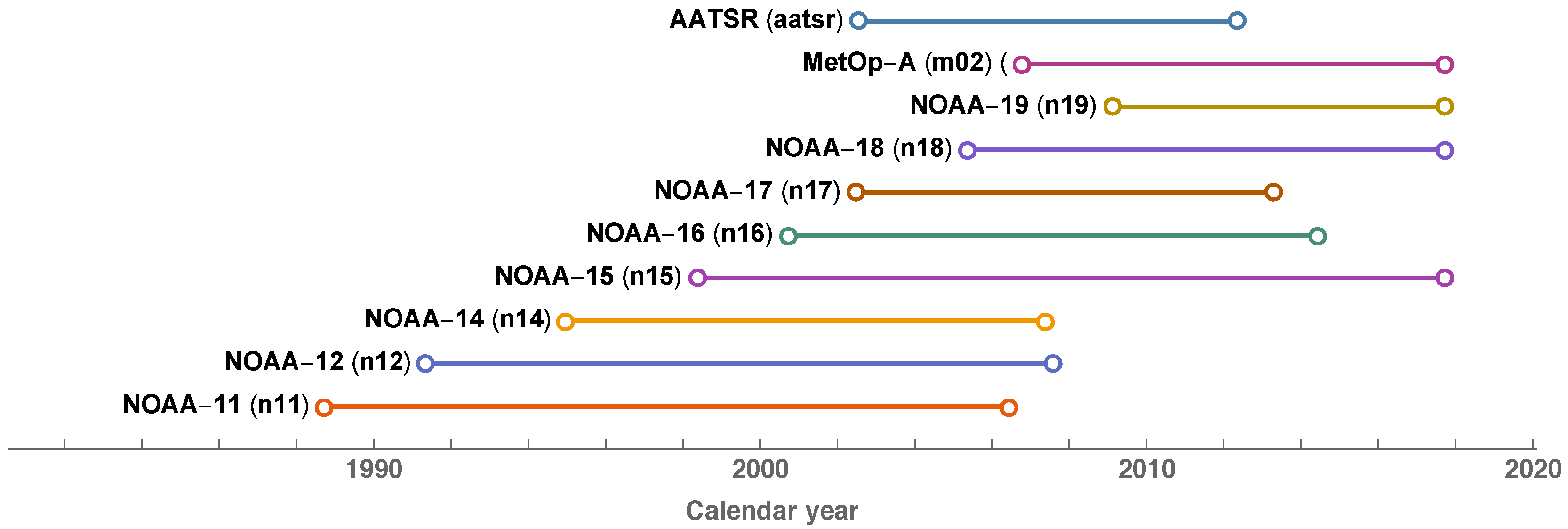
We have used the same measurement equation for all AVHRR sensors. Let ${\overline{C}}_{\mathrm{S}}$ and ${\overline{C}}_{\mathrm{ICT}}$ denote the sensor digital count numbers taken for the space view and the internal calibration target (ICT) that have resulted from a moving average of the respective direct measurements over several scan lines. Furthermore, let $C_{\mathrm{E}}$ denote the sensor digital count number directly taken for an Earth target, let $L_{\mathrm{ICT}}$ denote the radiance calculated (by means of Planck’s law and convolution with the sensor spectral response) from direct measurements of the ICT’s temperature, and let T denote the temperature of the instrument. Then, for each sensor i with telemetry data ${\mathit{x}}^i=({\overline{C}}_{\mathrm{S}}^i,{\overline{C}}_{\mathrm{ICT}}^i,C_{\mathrm{E}}^i,L_{\mathrm{ICT}}^i,T^i),$ the measurement equation is

$$L^i({\mathit{x}}^i,{\mathit{\alpha }}^i)={\alpha }_1^i+(ϵ+{\alpha }_2^i)L_{\mathrm{ICT}}^i\frac{C_{\mathrm{E}}^i-{\overline{C}}_{\mathrm{S}}^i}{{\overline{C}}_{\mathrm{ICT}}^i-{\overline{C}}_{\mathrm{S}}^i}+{\alpha }_3^i(C_{\mathrm{E}}^i-{\overline{C}}_{\mathrm{S}}^i)(C_{\mathrm{E}}^i-{\overline{C}}_{\mathrm{ICT}}^i)+{\alpha }_4^i\frac{T^i-295\mathrm{K}}{10\mathrm{K}},$$

(32)

where $ϵ$ is a constant that denotes the nominal emissivity of the internal calibration target. Note that we have neglected the radiance from space (negligible in comparison with radiance from the ICT) and that the instrument-temperature dependent term ${\alpha }_4^i{T}^i$ implicitly depends on the time of observation as the instrument temperature evolves over time with changes in the thermal environment.

Table 1. Nomenclature and error correlation structure of AVHRR telemetry data that has been taken into account.

Generic Name	Specific Name	Descriptive Name	Error Correlation Structure
$x_1$	${\overline{C}}_{\mathrm{S}}$	Space count average	structured random
$x_2$	${\overline{C}}_{\mathrm{ICT}}$	ICT count average	structured random
$x_3$	$C_{\mathrm{S}}$	Earth count	independent random
$x_4$	$L_{\mathrm{ICT}}$	ICT radiance	independent random
$x_5$	T	instrument temperature	independent random

summarises the nomenclature of AVHRR telemetry data and associated error correlation structures that we have assessed. Though in principle the measurements of ICT radiance exhibit all types of error correlation represented by Equations (7), (9) and (11), we have taken account of independent random errors only.

It is important to note that Equation (32) is invariant under any common random error in the measurements of instrument temperature $T^i$ because any correction to the instrument temperature term is already represented by the calibration parameter ${\alpha }_1^i$. Therefore, Equation (32) must not include additional calibration parameters to take account of (and estimate) these common random errors, and harmonisation should not consider them at all.

2.5. Satellite Data

We have considered the series of nine AVHRR sensors on-board the NOAA 11–19 and MetOp-A satellites to be harmonised with respect to the AATSR on-board Envisat as designated reference. The time lines of these satellite missions are illustrated in Figure 1. We have considered the period from 1991 to 2016 throughout which there were always two or more sensors in operation. AVHRR measures Earth TOA radiance in several wave bands. Here, we have examined the 11 $\mathsf{\mu }\mathrm{m}$ channel only for the AVHRR Global Area Coverage (GAC) data. The spectral response function for this instrument ranges from 10.3$\mathsf{\mu }\mathrm{m}$–11.3$\mathsf{\mu }\mathrm{m}$ and the resolution is 5 $\mathrm{k}$$\mathrm{m}$× 3 $\mathrm{k}$$\mathrm{m}$ around the sub-satellite point on ground. For examples of the AVHRR characteristics, see the NOAA KLM Guide [22].

Fundamental AVHRR telemetry data have been taken from the NOAA Comprehensive Large Array-data Stewardship System’s AVHRR Level 1B data and the AATSR reference TOA radiance data have been taken from the ESA AATSR Level 1 data. The reference uncertainty at the pixel level from the AATSR data has been taken to be of order 0.05 K [23]. The associated spatial resolutions have been assumed to be 1 $\mathrm{k}$$\mathrm{m}$ × 1 $\mathrm{k}$$\mathrm{m}$ at the sub-satellite point, and approximately 5 $\mathrm{k}$$\mathrm{m}$ × 3 $\mathrm{k}$$\mathrm{m}$ for the AVHRR GAC data. Note that, because one of the matchup criteria is to enforce a level of spatial uniformity in the observed field, any error introduced by possible mismatches between the AATSR and AVHRR footprints will also be included in the matchup uncertainty, which is primarily based on the local spatial variability.

Sensor-to-sensor matchups have been found automatically [24] under prescription of certain matchup selection criteria which are based on the criteria from the GSICS project [25]. First, the centre of each sensor’s field of view has to be concurrent so the two points are spatially consistent within the associated pixel footprint. Then, to minimise time variable differences between the matchups, we have used a time window of 300 s. We have also ensured parity in the viewing path length between the sensors and have used the difference in the path lengths of less than 1% as the selection criterion. Finally, we have enforced field uniformity to minimise errors due to geolocation errors and/or spatial inhomogeneity issues and have in this case used a threshold of 0.5 K for the spatial standard deviation in the AATSR pixels found in and around the AVHRR footprint.

A single matchup dataset has been created for each relevant pair of sensors.

Table 2. Number of sensor-to-sensor matchups selected for different pairs of satellites. Mnemonic names (see Figure 1) in the leading column refer to the first sensor i of a matchup dataset ${\mathit{M}}^{ij}$ while mnemonic names in the heading row refer to the second sensor j.

	Number of Matchups (Million)
	m02	n19	n18	n17	n16	n15	n14	n12	n11
aatsr	2.40	0.23	0.61	0.26	0.70	0.19	-	-	-
m02	-	2.20	2.72	2.13	1.75	1.43	-	-	-
n19	-	-	2.19	1.25	1.50	1.30	-	-	-
n18	-	-	-	2.26	2.64	1.45	-	-	-
n17	-	-	-	-	2.27	1.78	-	-	-
n16	-	-	-	-	-	2.09	-	-	-
n15	-	-	-	-	-	-	2.27	-	-
n14	-	-	-	-	-	-	-	2.38	-
n12	-	-	-	-	-	-	-	-	1.40

lists the number of matchups selected for each pair, adding up to about 40 million matchups in total. Error covariance information has been added to each matchup dataset in a way that evaluating Equations (7), (9) and (11) is straightforward. Weight matrices $\mathit{W}$ have been represented in compressed sparse row format [26].

For each pair of sensors, the expected radiance differences ${\mathit{K}}^{ij}$ and associated uncertainties $u({\mathit{K}}_{\mathrm{m}}^{ij})$ and $u({\mathit{K}}_{\mathrm{s}}^{ij})$ have been derived using a database of over a million Infrared Atmospheric Sounding Interferometer (IASI) spectra to represent variations in the observed TOA spectral radiance. For each instrument, the appropriate spectral response function has been used to integrate the IASI spectra to derive estimates of the respective infrared (IR) channel radiances. The expected difference in radiance for the 11 $\mathsf{\mu }\mathrm{m}$ channel between any two sensor pairs can then be directly estimated for that particular top of atmosphere spectrum. These differences are incorporated into a lookup table which is a function combining all three IR channels for night time matches (where solar scattering is not an issue) and using the two long wave IR channels during the day. Note that doing it this way ensures estimates of the channel-to-channel difference under both clear sky as well as cloudy conditions. The lookup table elements themselves contain the average 11 $\mathsf{\mu }\mathrm{m}$ channel difference together with an estimate of the standard deviation of the mean using the distribution of all difference estimates contained within that particular lookup table element. Those lookup table elements where there are insufficient difference estimates to provide a standard deviation are discarded.

3. Results

This section presents results on the harmonisation of a series of nine AVHRR sensors on-board the MetOp-A and NOAA 11–19 satellites with respect to the AATSR on-board Envisat as the designated reference. The MEIV technique has been applied to harmonise AVHRR 11 $\mathsf{\mu }$$\mathrm{m}$ TOA radiance as computed from sensor telemetry data by means of (32). The cost function includes about 40 million matchups, which requires less than 30 GB of memory on a single compute node to run the optimisation and to calculate the calibration parameter error covariance matrix. Exploiting eight concurrent threads to compute the cost function within each iteration, the optimisation takes less than 40 h on a single workstation with Intel (Santa Clara, CA, United States) Core i7-6700K CPU at a clock rate of $4.0$ $\mathrm{G}$$\mathrm{Hz}$. Calculating the parameter error covariance matrix takes about one hour. Results comprise harmonised calibration parameters, diagnostic diagrams, and a tentative stability analysis.

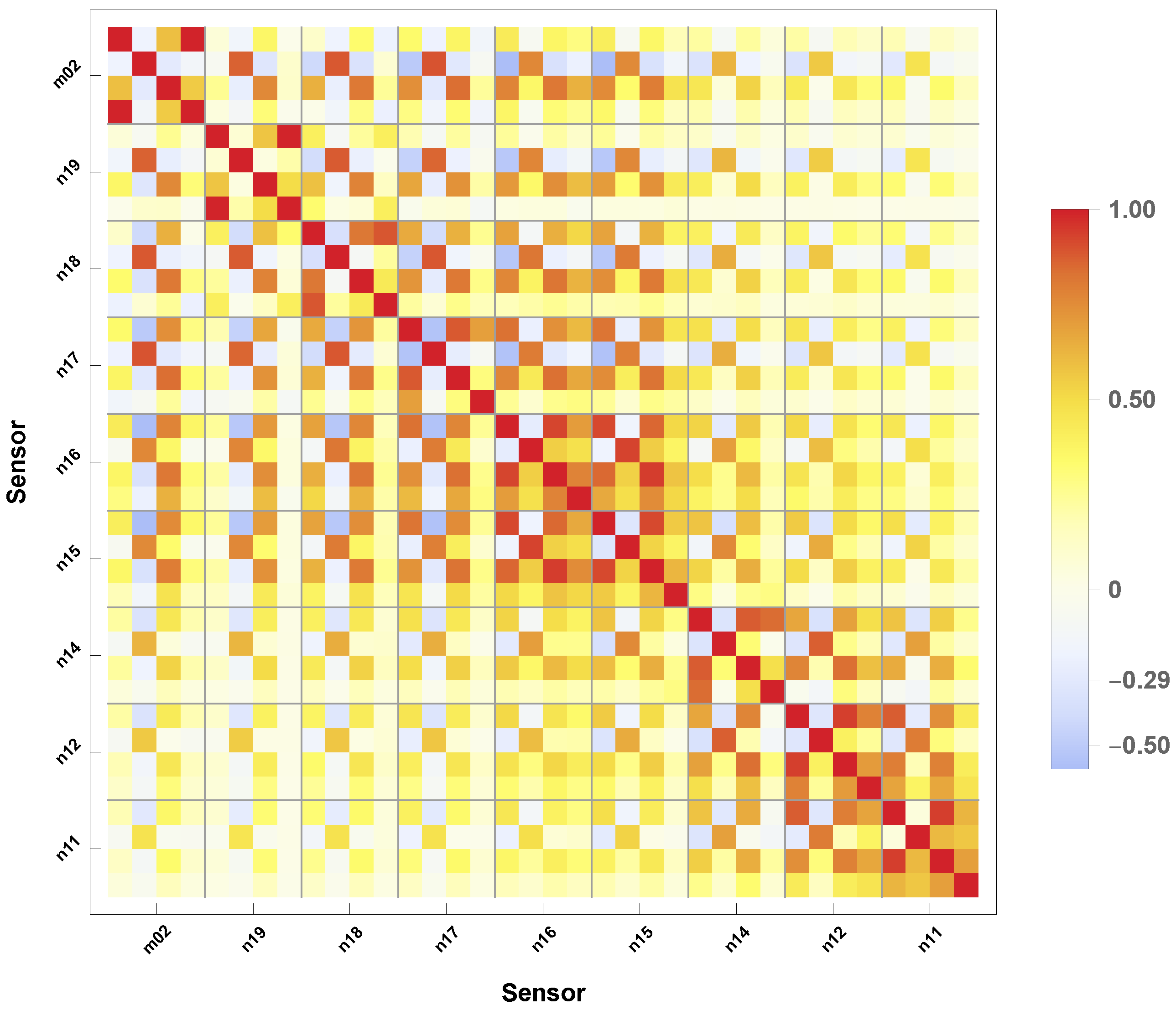
3.1. Harmonised Calibration Parameters

The harmonisation procedure optimised 36 calibration parameters $\mathit{\alpha }$, four calibration parameters for each AVHHR instrument considered, and calculated the calibration parameter error covariance matrix.

Table 3. Values of harmonised calibration parameters.

Satellite	Abbreviation	Calibration Coefficients
		${\widehat{\alpha }}_1$	${\widehat{\alpha }}_2$	${\widehat{\alpha }}_3$	${\widehat{\alpha }}_4$
		$\mathrm{m}\mathrm{W}{\mathrm{m}}^{-2}{\mathrm{sr}}^{-1}\mathrm{c}\mathrm{m}$	${10}^{-2}$	${10}^{-5}\mathrm{m}\mathrm{W}{\mathrm{m}}^{-2}{\mathrm{sr}}^{-1}\mathrm{c}\mathrm{m}$
MetOp-A	m02	$-4.4858\pm 0.0164$	$-0.1287\pm 0.0009$	$1.2690\pm 0.0014$	$-3.5116\pm 0.0181$
NOAA-19	n19	$-1.1419\pm 0.0102$	$-0.9817\pm 0.0010$	$1.5570\pm 0.0016$	$-2.9937\pm 0.0136$
NOAA-18	n18	$-2.9475\pm 0.0017$	$-0.9371\pm 0.0010$	$1.5083\pm 0.0014$	$-2.4684\pm 0.0017$
NOAA-17	n17	$-1.4091\pm 0.0012$	$-0.2653\pm 0.0010$	$2.0562\pm 0.0013$	$-0.0930\pm 0.0007$
NOAA-16	n16	$-1.2093\pm 0.0010$	$-1.2083\pm 0.0010$	$0.5737\pm 0.0013$	$-0.4956\pm 0.0004$
NOAA-15	n15	$-1.8321\pm 0.0009$	$-0.5223\pm 0.0010$	$1.0827\pm 0.0015$	$-0.4625\pm 0.0004$
NOAA-14	n14	$-2.0368\pm 0.0025$	$-1.6397\pm 0.0016$	$1.1948\pm 0.0021$	$-1.4038\pm 0.0024$
NOAA-12	n12	$-1.3174\pm 0.0024$	$-0.3173\pm 0.0020$	$1.5838\pm 0.0025$	$-0.0863\pm 0.0009$
NOAA-11	n11	$-1.8684\pm 0.0027$	$-0.9456\pm 0.0029$	$3.1294\pm 0.0041$	$-0.4772\pm 0.0010$

lists the harmonised calibration parameter values $\widehat{\mathit{\alpha }}$. Uncertainties have been obtained from the square root of the diagonal elements of the error covariance matrix. Note that the constraints on the calibration parameter ${\alpha }_4$ of the AVHRRs on board MetOp-A and NOAA-19 are relatively weak because the temperature of these instruments is very stable, i.e from 285.9 $\mathrm{K}$ to 286.4 $\mathrm{K}$ and from 286.9 $\mathrm{K}$ to 288.3 $\mathrm{K}$, respectively. The harmonised values of the calibration parameters ${\alpha }_1$ and ${\alpha }_4$ (and their errors) are therefore strongly correlated in the cases.

Figure 2 illustrates the posterior error correlation matrix of the harmonised calibration parameters, which has been derived from the error covariance matrix $\mathit{S}(\widehat{\mathit{\alpha }})$. The figure visualises intra- and inter-sensor error correlations. While the former emanate from the measurement equation itself, the latter originate from matchups of an AVHRR sensor with any other AVHRR sensor. The inter-sensor error correlation structure shown in Figure 2 is a direct implication of the structure and number of pairwise reference-to-sensor and sensor-to-sensor matchups listed in Table 2. Due to the sparse temporal overlapping between the later and the earlier AVHRRs (i.e., on board NOAA-11 to NOAA-14) the respective inter-sensor error correlations are relatively weak. Because the errors in the harmonised calibration parameters are strongly correlated, the full error covariance matrix (and not the mere diagonal variance elements only) must be considered in order to propagate calibration uncertainty to harmonised FCDR radiance.

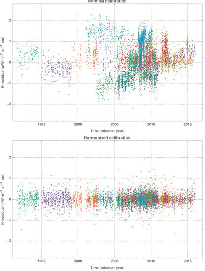
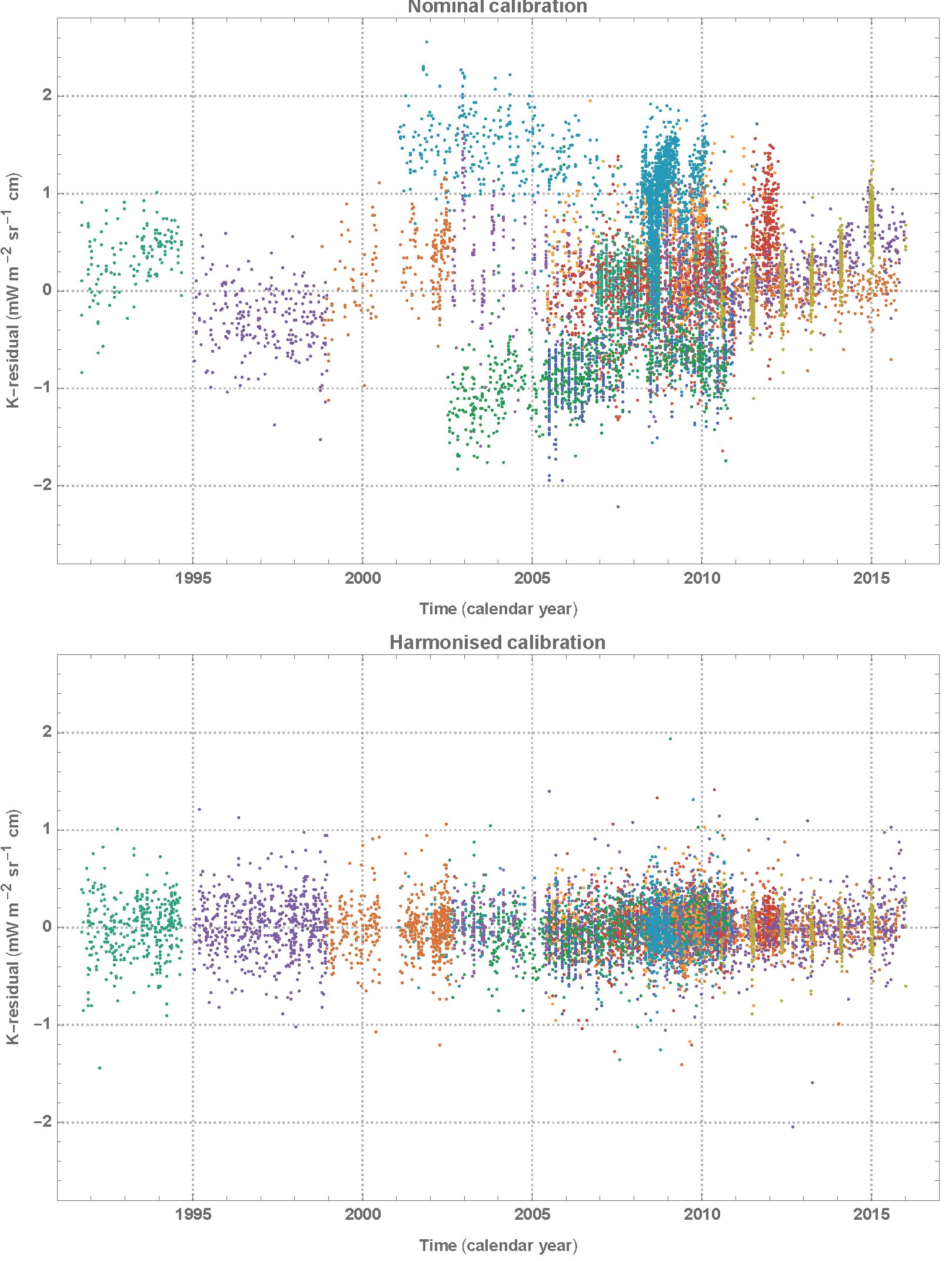
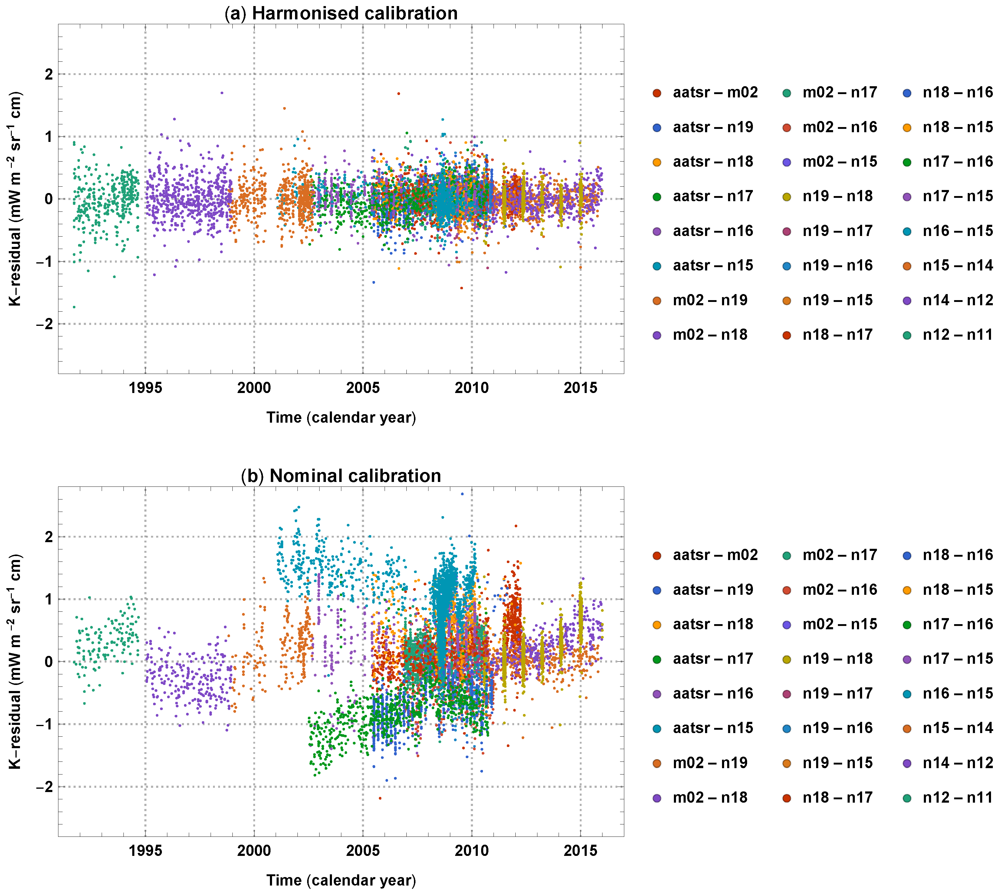
3.2. Diagnostic Diagrams

Figure 3 illustrates how the optimisation procedure (which initially started from $\mathit{\alpha }=0$) reduced the value of the cost function and after 1000 iterations converged at the harmonised calibration $\widehat{\mathit{\alpha }}$. If the measurement equation were a perfect representation of the instrument and errors in all matchup data were distributed normally and characterised perfectly well, the statistically expected value of the cost function at its minimum would be half the number of matchups, i.e., about 20 million. Figure 3 reveals that the actual minimum is less, i.e., about 13 million, which indicates that matchup data uncertainties may have been overestimated.

Figure 4 illustrates the mean and the standard deviation of the harmonised K-residual distribution for each sensor pair. If there were an issue with a certain sensor, this type of diagram would reveal it. Note that the magnitude of K-residuals (here and in other figures expressed in $\mathrm{m}\mathrm{W}{\mathrm{m}}^{-2}{\mathrm{sr}}^{-1}\mathrm{c}\mathrm{m}$) is approximately the same as the magnitude of corresponding brightness temperature difference (expressed in $\mathrm{K}$). That is to say most mean K-residuals differ by less than $0.02$ $\mathrm{K}$ and all differ by less than $0.06$ $\mathrm{K}$ from zero, the value expected if the calibration of each instrument were without fault.

Figure 5 depicts the probability distribution of harmonised K-residuals for all sensor pairs. This type of figure would reveal if the matchup data were affected by outliers or largely non-normal error statistics. The top panel of Figure 5 demonstrates that the distribution of K-residuals is a reasonable combination of a normal and a Laplace distribution and does not exhibit a significant fraction of statistical outliers. The mean of the K-residual distribution of −0.004 mW m⁻² sr⁻¹ cm is virtually zero, which would be expected if the harmonisation were perfect. The standard deviation of the K-residual distribution is −0.238 mW m⁻² sr⁻¹ cm, i.e., when expressed in brightness temperature, the dispersion of K-residuals is less than $0.3$ $\mathrm{K}$. The bottom panel of Figure 5 shows that the distribution of uncertainty-normalised K-residuals is more compact than a standard normal distribution, which they would be expected to follow if the overall uncertainty analysis were flawless. The more compact distribution of K-residuals seen may be explained by an overestimation of the uncertainties.

Figure 6 depicts the distribution of K-residuals over time. This type of diagram reveals when the matchup data are affected by temporary outliers and other particular error statistics, which do not appear in Figure 5. For instance, Figure 6 reveals some seasonal variations and demonstrates that the increase of dispersion of K-residuals in the years 2008 and 2009 arises from temporary issues in matches between the NOAA-16 and -15 satellites.

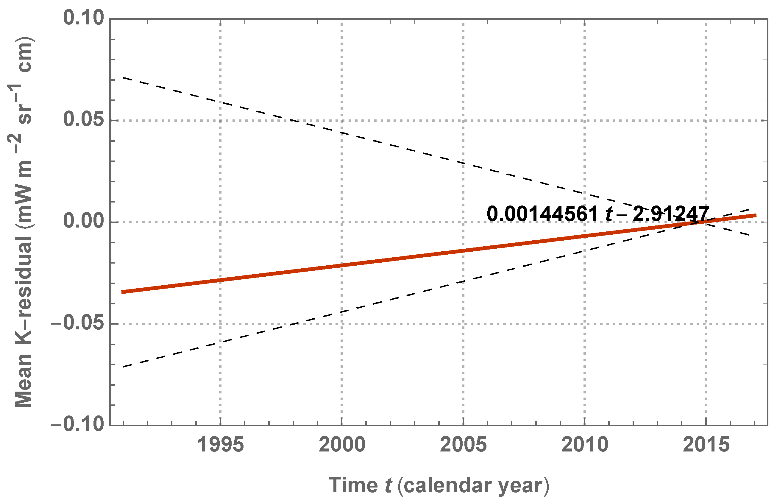
3.3. Stability of the Calibrated Radiance Data Record

The distribution of K-residuals over time (see Figure 6) may be used to infer the stability of the harmonised radiance data record. The top panel of Figure 7 illustrates the K-residuals for a subsample of matchups between all possible sensor pairs, with different sensor pairs marked by different colours. The subsample has been selected randomly from the distribution illustrated in Figure 6. The bottom panel of Figure 7 shows the K-residuals for the same matchups, but calculated from the nominal AVHRR calibration instead of the harmonised calibration. The mean K-residuals obtained from the nominal calibration exhibit mutual differences of 1–2 radiance units. Depending on the sensor pair considered, trends of mean K-residuals over time are sometimes positive and sometimes negative. The bottom panel of Figure 7 reveals the deficiencies of the nominal radiance calibration, which lead to highly unstable radiance data records that do meet climate data requirements. In contrast, the top panel of Figure 7 demonstrates that mutual differences of the mean harmonised K-residuals and their temporal trends are small, indicating a much better stability.

Figure 8 illustrates the trend of the mean harmonised K-residual from all sensor pairs over time, which is −0.0145 mW m⁻² sr⁻¹ cm decade⁻¹. Remembering that the magnitude of K-residuals is approximately the same as the magnitude of the corresponding brightness temperature difference, this trend roughly translates into $0.015$ $\mathrm{K}$ decade⁻¹ which is half the value tolerated by the requirement of the Global Climate Observing System (GCOS) on the stability of the Sea Surface Temperature essential climate variable [27]. Please note that this tentative stability analysis is based on matchup pairs, which are for the most part located in Arctic (Greenland) and Antarctic regions and do not constitute a globally-representative sample. The radiance samples from the selected matchups do, however, cover almost the complete range of observed radiances.

4. Discussion

We have presented a metrologically rigorous marginalised errors-in-variables (MEIV) approach to achieve a harmonised calibration of sensors onboard a series of Earth observation satellites. We have applied the method to harmonise TOA radiance from nine AVHRR sensors on board of NOAA and MetOp satellites with the AATSR reference. The harmonised calibration constitutes a significant improvement when compared to the nominal calibration in terms of stability over time, being roughly in the region of GCOS requirements. Matrix-free computations within the MEIV method allow for matchup datasets including several hundred million measurements, which enables calibration on the basis of even the noisiest telemetry. Most accurate and efficient computations involving first and second order partial derivatives have been enabled by means of advanced AD techniques [17,18,19,20,21], namely Transformation of Algorithms in Fortran [28]. The use of AD techniques enables quick trials of measurement equations with different or additional calibration parameters without the need to put any effort on programming partial derivative codes manually.

The mathematical framework presented in this paper is fully developed, but the harmonisation of the AVHRR series of sensors is ongoing. The Fidelity and Uncertainty in Climate data records from Earth observation (FIDUCEO) project [29] is refining the measurement equation, based on ongoing analyses of instrument characteristics and the results of the initial harmonised calibration presented in this study. Application of the MEIV method to harmonise the High-resolution Infrared Radiation Sounder (HIRS) series of sensors and the microwave sounders onboard NOAA and MetOp satellites is an ongoing activity within the FIDUCEO project too. Eventually, the harmonised calibration parameters will be used to produce new harmonised FCDRs, which include metrologically sound associated uncertainties per datum.

The MEIV framework is very generic. It may be configured to use a single reference sensor as in this study, but may readily use multiple reference sensors, which have already been harmonised too. Configuring calibration prior terms for designated reference sensors even allows for a harmonisation where the nominal calibration of the reference is updated with new information. Though the framework considers instrument channels individually, an obvious future extension of the framework may consider the calibration of multiple instrument channels in one go, e.g., to quantify inter-channel error correlation. On the other extreme, the framework may be configured to improve existing bias correction schemes (or sensor-equivalent calibration activities like GSICS [30]) which work on the basis of nominally calibrated radiance. Here, the improvement will be a (formally) correct consideration and propagation of radiance and bias correction uncertainty (which will not be an as complete and metrologically rigorous treatment as harmonisation, however).

With SI traceable satellites planned and launched in the future, harmonisation will have the potential to establish SI traceability for even heritage instruments, with the ultimate objective to produce SI traceable FCDRs extending over decades, ideally back to the beginning of Earth observation from Space.

References

1. Woolliams, E.R.; Mittaz, J.P.D.; Merchant, C.J.; Hunt, S.E.; Harris, P.M. Applying metrological techniques to satellite fundamental climate data records. J. Phys. Conf. Ser. 2018, 972, 012003. [Google Scholar] [CrossRef]
2. Mittaz, J.; Merchant, C.J.; Woolliams, E.R. Applying principles of metrology to historical Earth observations from satellites. Metrologia 2019. [Google Scholar] [CrossRef]
3. Merchant, C.J.; Holl, G.; Mittaz, J.P.D.; Woolliams, E.R. Radiance Uncertainty Characterisation to Facilitate Climate Data Record Creation. Remote Sens. 2019, 11, 474. [Google Scholar] [CrossRef]
4. Merchant, C.J.; Paul, F.; Popp, T.; Ablain, M.; Bontemps, S.; Defourny, P.; Hollmann, R.; Lavergne, T.; Laeng, A.; de Leeuw, G.; et al. Uncertainty information in climate data records from Earth observation. Earth Syst. Sci. Data 2017, 9, 511–527. [Google Scholar] [CrossRef]
5. Chander, G.; Hewison, T.J.; Fox, N.P.; Wu, X.; Xiong, X.; Blackwell, W.J. Overview of intercalibration of satellite instruments. IEEE Trans. Geosci. Remote Sens. 2013, 51, 1056–1080. [Google Scholar] [CrossRef]
6. Newey, W.K. Flexible simulated moment estimation of nonlinear errors-in-variables models. Rev. Econ. Stat. 2001, 83, 616–627. [Google Scholar] [CrossRef]
7. Zwolak, J.W.; Boggs, P.T.; Watson, L.T. Algorithm 869: ODRPACK95: A weighted orthogonal distance regression code with bound constraints. ACM Trans. Math. Softw. 2007, 33, 27. [Google Scholar] [CrossRef]
8. Hunt, S.E.; Quast, R.; Harris, P.M.; Mittaz, J.P.D.; Woolliams, E.R.; Giering, R.; Dilo, A.; Merchant, C.J. A metrological approach to producing harmonised fundamental climate data records from long-term sensor series data. In Proceedings of the IGARSS 2018—2018 IEEE International Geoscience and Remote Sensing Symposium, Valencia, Spain, 22–27 July 2018; pp. 3397–3400. [Google Scholar]
9. Harris, P.M.; Hunt, S.E.; Quast, R.; Giering, R.; Mittaz, J.P.D.; Woolliams, E.R.; Dilo, A.; Cox, M. Solving large structured non-linear least-squares problems with an application in Earth observation. in preparation.
10. Tarantola, A. Inverse Problem Theory and Methods for Model Parameter Estimation; Society for Industrial and Applied Mathematics (SIAM): Philadelphia, PA, USA, 2005. [Google Scholar]
11. Joint Committee for Guides in Metrology. Evaluation of Measurement Data. Guide to the Expression of Uncertainty in Measurement (JCGM 100:2008). Available online: http://www.bipm.org/en/publications/guides (accessed on 24 August 2018).
12. Griewank, A.; Walther, A. Evaluating Derivatives: Principles and Techniques of Algorithmic Differentiation, 2nd ed.; Number 105 in Other Titles in Applied Mathematics; SIAM: Philadelphia, PA, USA, 2008. [Google Scholar]
13. Barrett, R.; Berry, M.; Chan, T.F.; Demmel, J.; Donato, J.; Dongarra, J.; Eijkhout, V.; Pozo, R.; Romine, C.; van der Vorst, H. Templates for the Solution of Linear Systems: Building Blocks for Iterative Methods; Society for Industrial and Applied Mathematics (SIAM): Philadelphia, PA, USA, 1994. [Google Scholar]
14. Liu, D.C.; Nocedal, J. On the limited-memory BFGS method for large scale optimization. Math. Program. 1989, 45, 503–528. [Google Scholar] [CrossRef]
15. Zhu, C.; Byrd, R.H.; Lu, P.; Nocedal, J. Algorithm 778: L-BFGS-B: Fortran subroutines for large-scale bound-constrained optimization. ACM Trans. Math. Softw. 1997, 23, 550–560. [Google Scholar] [CrossRef]
16. Morales, J.L.; Nocedal, J. Remark on Algorithm 778: L-BFGS-B: Fortran Subroutines for Large-scale Bound Constrained Optimization. ACM Trans. Math. Softw. 2011, 38, 7:1–7:4. [Google Scholar] [CrossRef]
17. Giering, R.; Kaminski, T. Recipes for Adjoint Code Construction. ACM Trans. Math. Softw. 1998, 24, 437–474. [Google Scholar] [CrossRef]
18. Giering, R.; Kaminski, T. Applying TAF to generate efficient derivative code of Fortran 77–95 programs. In PAMM: Proceedings in Applied Mathematics and Mechanics; WILEY-VCH: Berlin, Germany, 2002. [Google Scholar]
19. Giering, R.; Kaminski, T. Recomputations in Reverse Mode AD. In Automatic Differentiation: From Simulation to Optimization; Corliss, G., Faure, C., Griewank, A., Hascoët, L., Naumann, U., Eds.; Computer and Information Science; Springer: New York, NY, USA, 2002; Chapter 33; pp. 283–291. [Google Scholar]
20. Giering, R.; Kaminski, T.; Slawig, T. Generating efficient derivative code with TAF. Future Gener. Comput. Syst. 2005, 21, 1345–1355. [Google Scholar] [CrossRef]
21. Giering, R.; Voßbeck, M. Increasing memory locality by executing several model instances simultaneously. In Recent Advances in Algorithmic Differentiation; Forth, S., Hovland, P., Phipps, E., Utke, J., Walther, A., Eds.; Springer: Berlin/Heidelberg, Germany, 2012; pp. 93–101. [Google Scholar]
22. NOAA KLM User’s Guide with NOAA-N, N Prime, and MetOp Supplements; National Oceanic and Atmospheric Administration: Washington, DC, USA, 2014.
23. Smith, D.; Mutlow, C.; Delderfield, J.; Watkins, B.; Mason, G. ATSR infrared radiometric calibration and in-orbit performance. Remote Sens. Environ. 2012, 116, 4–16. [Google Scholar] [CrossRef]
24. Block, T.; Embacher, S.; Merchant, C.J.; Donlon, C. High-performance software framework for the calculation of satellite-to-satellite data matchups (MMS version 1.2). Geosci. Model Dev. 2018, 11, 2419–2427. [Google Scholar] [CrossRef]
25. Wu, W.; Hewison, T.; Tahara, Y. GSICS GEO-LEO inter-calibration: Baseline algorithm and early results. In Atmospheric and Environmental Remote Sensing Data Processing and Utilization V: Readiness for GEOSS III; Springer: Berlin/Heidelberg, Germany, 2009; Volume 7456, pp. 745604-1–745604-12. [Google Scholar]
26. Saad, Y. Iterative Methods for Sparse Linear Systems, 2nd ed.; Society for Industrial and Applied Mathematics: Philadelphia, PA, USA, 2003. [Google Scholar]
27. NOAA. GCOS Ocean Physics ECV—Sea Surface Temperature. Available online: https://www.ncdc.noaa.gov/gosic/gcos-essential-climate-variable-ecv-data-access-matrix/gcos-ocean-physics-ecv-sea-surface-temperature (accessed on 14 February 2019).
28. FastOpt GmbH. Transformation of Algorithms in Fortran Demonstrator. Available online: http://www.fastopt.de/test/taf/tafdemo.html (accessed on 4 April 2019).
29. Fidelity and Uncertainty in Climate Data Records from Earth Observation (FIDUCEO). FIDUCEO Web Site. Available online: http://www.fiduceo.eu (accessed on 4 April 2019).
30. Global Space-based Inter-Calibration System (GSICS). GSICS Web Site. Available online: https://gsics.wmo.int (accessed on 4 April 2019).
Figure 1. Timeline of NOAA and MetOp satellites, which have all been equipped with similar sensors, like, e.g., the AVHRR. The AATSR sensor onboard the Envisat satellite was similar to the AVHRR.
Remotesensing 11 01002 g001
Figure 2. Error correlation matrix of harmonised calibration parameters. Thin horizontal and vertical lines separate the symmetric matrix into blocks of four by four pixels. Each block is associated with different sensors as indicated by mnemonic labels along the horizontal and vertical axis. Pixels inside diagonal blocks represent intra-sensor error correlations, whereas pixels inside off-diagonal blocks represent inter-sensor error correlations. Each off-diagonal pixel indicates how the errors in two different calibration parameters are correlated.
Remotesensing 11 01002 g002
Figure 3. Minimisation of the cost function.
Remotesensing 11 01002 g003
Figure 4. Mean and standard deviation of the harmonised K-residual distribution for each matchup dataset.
Remotesensing 11 01002 g004
Figure 5. (a) top panel: distribution of harmonised K-residuals for all sensor pairs. The solid and dashed lines mark normal and Laplace distributions, which have the same mean and the same dispersion as the distribution of K-residuals; (b) bottom panel: as above but showing the distribution of uncertainty-normalised K-residuals. The dotted curve marks the standard normal distribution.
Remotesensing 11 01002 g005
Figure 6. Probability density (indicated by logarithmic colour scale) of harmonised K-residuals over time. (a) top panel: for all sensor pairs; (b) bottom panel: for a specific sensor pair (here NOAA-16 and -15).
Remotesensing 11 01002 g006
Figure 7. Random sample of 10,000 matchups from all sensor pairs. (a) top panel: K-residuals calculated from the harmonised calibration; (b) bottom panel: the same samples, but calculated from the nominal AVHRR calibration.
Remotesensing 11 01002 g007
Figure 8. Trend of the mean harmonised K-residual from all sensor pairs over time. Dashed lines roughly indicate the requirement of GCOS on the decadal stability of the Sea Surface Temperature essential climate variable, which is 0.03 K decade−1 [27].
Remotesensing 11 01002 g008