Research on Time-Correlated Errors Using Allan Variance in a Kalman Filter Applicable to Vector-Tracking-Based GNSS Software-Defined Receiver for Autonomous Ground Vehicle Navigation

Abstract

The global navigation satellite system (GNSS) has been applied to many areas, e.g., the autonomous ground vehicle, unmanned aerial vehicle (UAV), precision agriculture, smart city, and the GNSS-reflectometry (GNSS-R), being of considerable significance over the past few decades. Unfortunately, the GNSS signal performance has the high risk of being reduced by the environmental interference. The vector tracking (VT) technique is promising to enhance the robustness in high dynamics as well as improve the sensitivity against the weak environment of the GNSS receiver. However, the time-correlated error coupled in the receiver clock estimations in terms of the VT loop can decrease the accuracy of the navigation solution. There are few works present dealing with this issue. In this work, the Allan variance is accordingly exploited to specify a model which is expected to account for this type of error based on the 1st-order Gauss-Markov (GM) process. Then, it is used for proposing an enhanced Kalman filter (KF) by which this error can be suppressed. Furthermore, the proposed system model makes use of the innovation sequence so that the process covariance matrix can be adaptively adjusted and updated. The field tests demonstrate the performance of the proposed adaptive vector-tracking time-correlated error suppressed Kalman filter (A-VTTCES-KF). When compared with the results produced by the ordinary adaptive KF algorithm in terms of the VT loop, the real-time kinematic (RTK) positioning and code-based differential global positioning system (DGPS) positioning accuracies have been improved by 14.17% and 9.73%, respectively. On the other hand, the RTK positioning performance has been increased by maximum 21.40% when compared with the results obtained from the commercial low-cost U-Blox receiver.

1. Introduction

The application of the global navigation satellite system (GNSS) has had considerable significance during the past two decades for positioning and navigation in terms of the autonomous ground vehicle [1,2,3,4], unmanned aerial vehicle (UAV) [5,6,7], precision farming [8,9,10,11], smart city relied on information and communication technology (ICT) [12,13,14] and internet of things (IoT) [15,16,17], as well as for the GNSS-reflectometry (GNSS-R) towards agriculture [18,19], forest monitoring [20], wind geophysical modeling [21], sea ice remote sensing [22], and its other improved algorithms [23,24]. The GNSS receiver plays a very significant role of being integrated with other sensors, e.g., inertial navigation system (INS) [25], odometer [26], light detection and ranging (LiDAR) or laser scanner [27], camera [28], as well as the GNSS signal is promising to be jointed with the other satellite signals, e.g., synthetic aperture radar (SAR) [29,30], to provide the accurate and continuous absolute navigation solutions. Besides, the concept of position dilution of precision (PDOP) which is originated from the GNSS positioning technique is also exploited by Hu et al. to propose an optimal approach enabling an improvement of the three-dimensional (3D) deformation retrieval accuracy with respect to the SAR signal [31].

1.1. Challenges for The GNSS Receiver

Many difficulties will be encountered by the GNSS signal through its transmission in the atmosphere. It should be noted that the atmospheric noise not only reduces the signals from the GNSS satellites [32,33,34], but also the SAR signals whose performances may be largely reduced when they pass through the ionospheric and tropospheric layers and influenced by the turbulent atmosphere [29,35,36,37]. The ionospheric modelling is considerably a tricky issue towards the orbital satellite signal processing, and the signal power would be dramatically attenuated by the unintentional turbulence. The multipath interference forms another large challenge faced by the GNSS signal, since it randomly occurs. It is a type of biased error source that is hard to be modelled as well [38,39,40,41]. If the incoming signal is influenced due to the previously mentioned interference, the received signal strength may be highly attenuated and such weak signal is extremely hard to be handled through the baseband signal processing of the GNSS receiver. In addition, when the GNSS receiver are faced with the dynamic situation, the less accurate measurements can be produced as well referring to the characteristics of the loop filter in terms of the receiver tracking procedure [42]. It is worth noticing that such application towards increasing the performance of the dynamic GNSS signal processing is also embraced with great significance for some aerial system applications, e.g., mapping with unmanned aerial system [43] and airborne radiometric surveys [44]. Some advanced techniques have been recently presented to deal with the these challenging signals [32,45,46]. The vector tracking (VT) technique is capable of remarkably improving the performance on the GNSS signal processing in weak and dynamic environments with the assistance of the position and velocity solutions.

1.2. Vector Tracking Techniques for GNSS Receiver Design

The concept related to the vector delay lock loop (VDLL) which is assumed as the prototype of the VT structure for the tracking loop towards the GNSS receiver design was initially presented by Spilker [47]. Over the past several years, the VT technique has been accounted for many researchers’ interests embracing the objectives to enhance the ability of the receiver on weak and dynamic signal tracking [48,49], interference anti-jamming [50,51] as well as the multipath mitigation [52,53]. The researchers from the Position, Location And Navigation (PLAN) group of the University of Calgary have gained many achievements of working on the VT technique [50,54,55,56]. The strengths and drawbacks of the VT technique have been thoroughly analyzed in their publications, and many practical applications based on the VT architectures have been realized with the GNSS software-defined receiver (SDR) [49,57,58]. Many academic works have been published by Bhattacharyya who was from University of Minnesota, and these publications have provided the exhaustive analysis towards the receiver autonomous integrity monitoring (RAIM) algorithm for the VT loop [59,60,61]. The random noise in the navigation solutions produced by the VT architecture is the sum of the statistics data associated with the current epoch plus several past epochs. It has been mentioned in her dissertation that the time correlated errors related to the atmospheric delay residuals, ephemeris, multipath as well as the local clock estimations have to be appropriately modelled, and then it will be exploited to compensate such bias error present in the positioning solutions [59]. Accordingly, the researchers from the PLAN group propose an algorithm to improve the Kalman filter (KF) to deal with the time-correlated error in terms of the multipath interference coupled in the measurements [62]. Assuming that the time-correlated error due to the multipath error can be removed by the improved KF technique, there are still remained time-correlated errors in the VT loop caused by the statistical data from the local clock estimations, and these sorts of errors will be not present in the traditional scalar tracking (ST) loop. There are few papers published dealing with such time-correlated error.

1.3. Allan Variance Approaches towards Noise Source Modelling

Allan variance was developed by David W. Allan in 1966 [63] to specify an idea that an invariant measure for a quality factor in terms of a frequency standard can be determined by driving the canonical transformation of the power for the source of white noise [64]. The high similarities in analogies between the inertial sensors and Allan variance account for the application that the method has been adopted to analyze the characterization of random drift error in various devices [65]. It is also frequently applied to come up with the instability characteristics of precision oscillators [66]. It is worth noting that the generalized method of wavelets moments (GMWM) has recently been used for the modelling of inertial sensor errors [67] and GNSS positioning errors [68] as well. However, the Allan variance tool is adequate to be capable of identifying the error distribution in this research. The way to use GMWM quantifying the local clock error model of the GNSS receiver may be achieved in the future. In this work, the outcomes of Allan variance are corresponded to four basic distributions of the noise terms existing in local receiver clock and vector tracking loop of the GNSS SDR, i.e., white frequency, random walk frequency, flicker noise and exponentially correlated or Markov noise.

1.4. Summary

Our purpose in this work is to model the time-correlated error coupled in the clock drift estimations in the VT loop using the Allan variance. Then, an improved KF will be proposed based on the model. Furthermore, the field test experiments will demonstrate the performance of the proposed algorithms. More specific explanations will be described in the subsequent sections.

The remaining of this paper is organized as follows. Section 2 introduces the process of modelling the proposed adaptive vector-tracking time-correlated error suppressed Kalman filter (A-VTTCES-KF) including the basic concepts of the Allan variance, power spectrum density (PSD) related to the clock estimation random noise, time-correlated error model based on 1st-order Gauss-Markov (GM) process, the system model of the A-VTTCES-KF, the adaptive algorithm in terms of the process covariance matrix, and the numerically controlled oscillator (NCO) updating method; the field test results, using the GNSS SDR with the proposed A-VTTCES-KF algorithms plus the ordinary adaptive KF algorithms, and the commercial U-Blox receiver, are provided in Section 3; Section 4 is devoted to some analysis and discussions associated with the field test results; the last Section 5 concludes this work.

2. Materials and Methods

The system model of the proposed A-VTTCES-KF algorithm, and the introduction of the GNSS SDR based on the proposed methods will be introduced in this section. Some related fundamental materials and methods will be stated in the appendices, including the concept of the Allan variance method in Appendix A, local clock modelling in Appendix B, GM process in Appendix C. It should be mentioned that the 1st-order GM process will be subsequently adopted to model the time-correlated error related to the VT algorithm in this work.

2.1. A-VTTCES-KF Algorithm

In this section, the noise terms in the clock drift estimations of the GNSS SDR are identified and quantified with the Allan variance. Some preliminary experiments are firstly conducted to provide an exhaustive analysis on what types of error sources influence the performance of the NCO in a VT architecture. Then, the time-correlated error due to the VT algorithm will be modelled with the 1st-order GM process. Finally, an A-VTTCES-KF algorithm will be proposed to reduce the influence of the time-correlated error on the VT loop.

2.1.1. Preliminary Results and Analysis through Stationary Field Tests

• Vector tracking algorithms for stationary field tests
  The navigator will be formed with the weighted non-linear least square (WNLS) method [42] to provide the user’s position, velocity, and timing (PVT) estimations in the stationary field tests. It has been mostly accepted that the weighted matrix for the PVT estimation relies on the elevation angle of each satellite which corresponds to the priori variances for the measurements. The priori variance model is given by [69]

  $${\sigma }^2=\frac{{\sigma }_0^2}{{sin}^2\left(\gamma \right)}$$

  (1)

  where ${\sigma }_0$ is assumed to be the standard deviation (STD) of the pseudo-range measurement or Doppler measurement, and it will be set to 1 in our work; $\gamma$ stands for the elevation angle of a satellite in radians. Since the random noise on the PVT solution estimation at each epoch is independent and uncorrelated, it can be exploited to identify the characterization of the noise distribution by excluding the cross-correlation of the measurements in the VT loop through this condition. The architecture of the VT-based SDR is illustrated in Figure 1, where red lines denote the VT feedbacks, blue blocks represent the satellite vehicle (SV) ephemeris and the implementations which rely on ephemeris, DCM stands for the direction cosine matrix which includes unit vectors between the user and the line-of-sight (LOS) satellites, LR stands for the loop rate of the update.
  Since the VT architecture based on the WNLS navigator is not our contribution, the system model associated with this algorithm can be referred to the conference paper [70], and it will not be investigated and stated in this work.
• Setup for the field tests
  The radio frequency (RF) L1 C/A signal of the global positioning system (GPS) will be received through a single-frequency NovAtel antenna. The radio-frequency GNSS signal cannot be processed by the GNSS SDR unless it would be down-converted to the intermediate frequency (IF). In this research, a Fraunhofer GNSS front-end will be utilized to implement such procedure. A low-cost commercial U-Blox GNSS receiver was receiving the incoming signals using the same antenna as which was involved with the GNSS front-end. These two devices are connected with the antenna through a splitter and several radio-frequency cables. In addition, the high-performance multi-frequencies and multi-systems Trimble R10 receiver is set up next to the NovAtel antenna so that a high-accuracy trajectory related to the tested ground vehicle can be referred to. It should be known that, the reference receiver receives the GNSS signal with a separate antenna integrated in its body. The setup for all the field tests in this research is provided in Figure 2.
  Two open-sky scenarios are applied in the experiments to allow the implementation of the VT-based SDR in a stationary condition. In order to exclude the influence of the kinematic movement of the receiver on the clock error estimations, i.e., clock bias and clock drift errors, the preliminary experiments should be carried out in a stationary situation. Furthermore, the WNLS method instead of the KF algorithm is chosen to compute the PVT solutions to update the VT loop parameters such that the outputs of the navigator can be confirmed to be independent during the whole time spanning. The stationary experiments have been done in two situations in this work. The scenarios for Situation #1 and Situation #2 associated with the open-sky testing spot and the sky plot of the SVs are illustrated in Figure 3 and Figure 4, respectively. The clock drift estimations of the GNSS SDR through these two situations will be subsequently analyzed with the tool of Allan variance. The time-correlated error source which is coupled in the clock drift error is expected to be specified in this way.
• VT time-correlated error modelling based on Allan variance
  As mentioned earlier, two groups of the stationary experiments have been done to help identify and quantify the characteristics of the VT loop in terms of the time-correlated error. The estimation series of the clock drift can be estimated by the Doppler measurements through the WNLS method. The tests are carried out with different feedback modes. For example, the VT feedback intervals which range from 50 ms to 1000 ms are combined with different scales of the bandwidths for the 3rd-order phase lock loop (PLL), i.e., 1 Hz, 3 Hz, and 5 Hz. The feedback interval is the reciprocal of the LR as mentioned earlier. The results of the clock drift estimations related to Allan variance or Allan deviation for Situation #1 and Situation #2 are illustrated in Figure 5 and Figure 6, respectively. Some annotations have been depicted in the legends of these two figures as the format of ${\tau }_l$-$B_{pll}$, where ${\tau }_l$ denotes the VT feedback interval in millisecond, and $B_{pll}$ stands for the bandwidth of the PLL in Hertz; st in the legends means that the ST mode is activated in the test.
  Comparing the curves out of the ST loop with the ones from all the tested VT loops shown in Figure 5 and Figure 6, it should be noted that there is a distinctive segment appearing in the VT curves. The shape of this sort of segment is very close to the curve in Figure A3. Such similarity implies that the VT loop brings in a certain time-correlated error which is coupled in the clock drift estimations of the GNSS receiver. As we know, the performance of the tracking loop based on the VT technique is highly dependent on the quality of the clock drift estimations, and it can be inferred that the accuracy of the PVT solution for the receiver will certainly be reduced by this sort of the time-correlated disturbance error.
  Referring to the curves in Figure 5 and Figure 6, and (A13), the parameters for Markov process in different cases of the VT architectures can be approximated as the numerical values in

  Table 1. Summary of the parameters in terms of the Markov process or the time-correlated error source caused by the VT loop for Situation #1.

  ${\mathit{B}}_{\mathit{pll}}$ [Hz]	VT LR [Hz]	${\overline{\mathit{x}}}_{\mathit{GM}}$ [s]	${\overline{\mathit{y}}}_{\mathit{GM}}$ [s/s]	${\mathit{q}}_{\mathit{c}}$ [s/s]	${\mathit{T}}_{\mathit{c}}$ [s]
  5	20	0.130	$2.34\times {10}^{-10}$	$2.04\times {10}^{-9}$	0.069
  	10	0.170	$1.92\times {10}^{-10}$	$1.46\times {10}^{-9}$	0.090
  	5	0.200	$1.77\times {10}^{-10}$	$1.25\times {10}^{-9}$	0.106
  	2	0.275	$1.60\times {10}^{-10}$	$9.60\times {10}^{-10}$	0.146
  	1	0.330	$1.57\times {10}^{-10}$	$8.58\times {10}^{-10}$	0.175
  3	20	0.180	$2.40\times {10}^{-10}$	$1.78\times {10}^{-9}$	0.095
  	10	0.240	$1.90\times {10}^{-10}$	$1.22\times {10}^{-9}$	0.127
  	5	0.310	$1.68\times {10}^{-10}$	$9.46\times {10}^{-10}$	0.164
  	2	0.445	$1.54\times {10}^{-10}$	$7.26\times {10}^{-10}$	0.235
  	1	0.510	$1.53\times {10}^{-10}$	$6.72\times {10}^{-10}$	0.270
  1	20	0.310	$2.90\times {10}^{-10}$	$1.64\times {10}^{-9}$	0.164
  	10	0.445	$2.10\times {10}^{-10}$	$9.89\times {10}^{-10}$	0.235
  	5	0.630	$1.77\times {10}^{-10}$	$7.02\times {10}^{-10}$	0.333
  	2	1.055	$1.53\times {10}^{-10}$	$4.68\times {10}^{-10}$	0.558
  	1	N/A	N/A	N/A	N/A

  and

  Table 2. Summary of the parameters in terms of the Markov process or the time-correlated error source caused by the VT loop for Situation #2.

  ${\mathit{B}}_{\mathit{pll}}$ [Hz]	VT LR [Hz]	${\overline{\mathit{x}}}_{\mathit{GM}}$ [s]	${\overline{\mathit{y}}}_{\mathit{GM}}$ [s/s]	${\mathit{q}}_{\mathit{c}}$ [s/s]	${\mathit{T}}_{\mathit{c}}$ [s]
  5	20	0.135	$2.70\times {10}^{-10}$	$2.31\times {10}^{-9}$	0.071
  	10	0.160	$2.05\times {10}^{-10}$	$1.61\times {10}^{-9}$	0.085
  	5	0.190	$1.85\times {10}^{-10}$	$1.34\times {10}^{-9}$	0.101
  	2	0.240	$1.70\times {10}^{-10}$	$1.09\times {10}^{-9}$	0.127
  	1	0.295	$1.52\times {10}^{-10}$	$8.80\times {10}^{-10}$	0.156
  3	20	0.175	$2.88\times {10}^{-10}$	$2.16\times {10}^{-9}$	0.093
  	10	0.230	$1.97\times {10}^{-10}$	$1.29\times {10}^{-9}$	0.122
  	5	0.265	$1.66\times {10}^{-10}$	$1.01\times {10}^{-9}$	0.14
  	2	0.375	$1.56\times {10}^{-10}$	$8.01\times {10}^{-10}$	0.198
  	1	0.590	$1.40\times {10}^{-10}$	$5.73\times {10}^{-10}$	0.312
  1	20	0.305	$2.87\times {10}^{-10}$	$1.63\times {10}^{-9}$	0.161
  	10	0.445	$1.91\times {10}^{-10}$	$9.00\times {10}^{-10}$	0.235
  	5	0.685	$1.68\times {10}^{-10}$	$6.37\times {10}^{-10}$	0.362
  	2	0.970	$1.48\times {10}^{-10}$	$4.73\times {10}^{-10}$	0.513
  	1	N/A	N/A	N/A	N/A

  which are summarized for Situation #1 and Situation #2, respectively; ${\overline{x}}_{GM}$ and ${\overline{y}}_{GM}$ represent the time cluster and Allan deviation with respect to the peak of the Allan deviation plot, respectively, and they can be approximately read from the given plots; $q_c$ and $T_c$ can be referred to (A11) as well as the descriptions below for detailed information. Furthermore, $q_c$ and $T_c$ can be calculated through ${\overline{x}}_{GM}$ and ${\overline{y}}_{GM}$ estimations based on (A13).
  As listed in Table 1 and Table 2, it can be found that the parameters in terms of the same VT settings in two situations are very close to each other such that they can be exploited to build up a model to reduce the Markov process or time-correlated error disturbance on the VT tracking loop. The way to build up the system model will be subsequently explained. On the other hand, it can be noticed that, as ${\tau }_l$ = 1000 ms and $B_{pll}$ = 1 Hz, there are some other unexpected noise sources added into the Allan deviation plot of the VT-based clock drift error estimations. Since the dynamic stress on the tracking loop may be not adequately removed by the very slow feedback rate in terms of the LOS Doppler compensation combined with the user’s and the SV’s velocities. In this case, the Allan deviation curve might be dramatically contaminated by the dynamic stress residuals. However, analysis for this type of noise term is not our contribution in this research, it will not be discussed in this paper.
• Clock modelling based on Allan variance
  The curve of the timing stability for the local clock integrated in the front-end for the GNSS SDR is plot in Figure 7 by which the clock drift characteristics can be studied and depicted [63]. The test spot related to Situation #3 is given in Figure 10 in Section 3. Referring to Figure 7, the coefficient of the clock drift random walk can be estimated by (A8) with $\tau =1$, and the numerical value is approximated as $7.675\times {10}^{-11}$; the coefficient related to the rate of the clock drift random walk will be obtained from (A10) with $\tau =3$, and the numerical approximation is estimated as $1.069\times {10}^{-10}$. The flicker noise terms related to the flat segment will be not contained in the subsequent system model for the KF, and this omission is reasonable referring to previous researches [66].

It has been studied through previous mathematical analysis and experimental implementations, that the PSD related to the noise with the highly stable frequency terms can be expressed by a power-law noise model as follow [71,72]

$$S_y\left(f\right)=\sum _{\alpha =-2}^{+2}{h}_{\alpha }{f}^{\alpha }$$

(2)

subject to $0\le f\le f_h$, where the PSD varies with the variable of f which is corresponded to the signal power, and $f_h$ stands for the upper bound of the cutoff frequency; $h_{\alpha }$ is an amplitude coefficient [73] by which the range of f can be constrained; every separate numerical value of $\alpha$ corresponds to an existing noise source in the signal. The noise sources of white frequency and random walk frequency, which corresponds to $\alpha =0$ and $\alpha =-2$, respectively, will be subsequently taken into consideration for the receiver clock noise modelling. These two noise sources are more than enough to afford a stochastic model of the receiver clock [66].

Table 3. Summary for the Allan variance ${\sigma }^2\left(\tau \right)$ analysis of the noise [64,71,72].

Noise Source	General Model	Power-Law Model
White Frequency	$\frac{Q^2}{\tau }$	$\frac{h_0}{2\tau }$
Random Walk Frequency	$\frac{K^2\tau }{3}$	$\frac{{\left(2\pi \right)}^2\tau h_{-2}}{6}$

summaries the Allan variance results related to different types of coefficients.

In Table 3, the coefficient for the white frequency term in the noise of the clock drift is estimated as $Q=7.675\times {10}^{-11}$, while the coefficient for the random walk frequency term can be approximated as $K=1.069\times {10}^{-10}$, as illustrated in Figure 7. Under this circumstance, the amplitude coefficients in terms of the power-law model can be attained as

$$\left\{\begin{array}{c}{\widehat{h}}_0=2Q^2\approx 1.178\times {10}^{-20}\hfill \\ {\widehat{h}}_{-2}=\frac{K^2}{2{\pi }^2}\approx 5.789\times {10}^{-22}\hfill \end{array}\right.$$

(3)

According to the results of (3) and typical Allan variance coefficients stated in the previous work [66], the local clock integrated in the GNSS Fraunhofer front-end is better than the low-quality temperature compensated crystal (TCXO) but worse than the high-quality TCXO.

2.1.2. System Model for A-VTTCES-KF

Based on the earlier stationary experiments and related analysis, when the VT mode is activated, an extra source error, of which the Allan variance curve is very close to the shape of the Markov process as shown in Figure A3, appears in the clock drift estimations compared with the ST results. This fact leads to the consequence of the case that there is a type time-correlated bias coupled in the local clock errors in the VT loop, and such error would certainly contaminate the GNSS measurements, i.e., Doppler, carrier phase, and pseudo-range, through the tracking process. In this case, the performance of the advanced VT architecture can be reduced by this unexpected error. In this work, we are trying to implement an improved KF algorithm targeting to the suppression of the time-correlated error.

The discrete form of the dynamic process in terms of the navigation solutions can be described by the following equation

$$\delta {\mathbf{x}}_k={\mathsf{\Phi }}_{k,k-1}\delta {\mathbf{x}}_{k-1}+{\mathbf{w}}_{k-1}$$

(4)

Also, the observation process can be expressed as

$$\delta {\mathbf{z}}_k={\mathbf{H}}_k\delta {\mathbf{x}}_k+{\mathbf{v}}_k$$

(5)

where subscript k represents the index of the discrete samples; ${\mathsf{\Phi }}_{k,k-1}$ denotes the transition matrix from the epoch of $\left(k-1\right)$ to the k th epoch; ${\mathbf{H}}_k$ is the observation design matrix; $\delta {\mathbf{x}}_k$ and $\delta {\mathbf{z}}_k$ represent the state vector and observation vector, respectively; ${\mathbf{v}}_k$ and ${\mathbf{w}}_k$ represent the observation and the process random noise vectors, respectively, and they should be subject to

$$\left\{\begin{array}{c}\mathbf{E}\left[{\mathbf{w}}_k\right]=\mathbf{0},\mathbf{E}\left[{\mathbf{v}}_k\right]=\mathbf{0}\hfill \\ \mathbf{E}\left[{\mathbf{w}}_k{\mathbf{w}}_k^T\right]={\mathbf{Q}}_k,\mathbf{E}\left[{\mathbf{v}}_k{\mathbf{v}}_k^T\right]={\mathbf{R}}_k,\hfill \\ \mathbf{E}\left[{\mathbf{w}}_k{\mathbf{v}}_j^T\right]=\mathbf{0},k\ne j\hfill \end{array}\right.$$

(6)

with $k,j\in {\mathbb{Z}}^{+}$, where ${\mathbf{Q}}_k$ denotes the process covariance matrix, ${\mathbf{R}}_k$ represents the observation covariance matrix.

• State vector
  When the VT loop is working, the existing time-correlated error in the local clock drift estimation series is assumed to follow the 1st-order GM process in this research, and the system model is given by (A18). Then, the state vector for the proposed A-VTTCES-KF is given as follow

  $$\delta {\mathbf{x}}_k={\left[\begin{array}{c}\delta r_x\\ \delta r_y\\ \delta r_z\\ \delta v_x\\ \delta v_y\\ \delta v_z\\ \delta a_x\\ \delta a_y\\ \delta a_z\\ \delta b_c\\ \delta d_c\\ \delta \eta \end{array}\right]}_k=\left[\begin{array}{c}\mathrm{x}-\mathrm{axis}\mathrm{position}\mathrm{error}\\ \mathrm{y}-\mathrm{axis}\mathrm{position}\mathrm{error}\\ \mathrm{z}-\mathrm{axis}\mathrm{position}\mathrm{error}\\ \mathrm{x}-\mathrm{axis}\mathrm{velocity}\mathrm{error}\\ \mathrm{y}-\mathrm{axis}\mathrm{velocity}\mathrm{error}\\ \mathrm{z}-\mathrm{axis}\mathrm{velocity}\mathrm{error}\\ \mathrm{x}-\mathrm{axis}\mathrm{acceleration}\mathrm{error}\\ \mathrm{y}-\mathrm{axis}\mathrm{acceleration}\mathrm{error}\\ \mathrm{z}-\mathrm{axis}\mathrm{acceleration}\mathrm{error}\\ \mathrm{clock}\mathrm{bias}\mathrm{error}\\ \mathrm{clock}\mathrm{drift}\mathrm{error}\\ \mathrm{time}-\mathrm{correlated}\mathrm{error}\mathrm{difference}\end{array}\right]$$

  (7)

  where $\delta {\eta }_k={\eta }_k-{\eta }_{k-1}$; ${\eta }_k$ is assumed to follow the 1st-order GM process, and it is given by

  $${\eta }_k=e^{-\beta \mathsf{\Delta }t}{\eta }_{k-1}+W_{k-1}$$

  (8)

  with $\mathbf{E}\left(W_k\right)=0$ and $Q_W=\mathbf{E}\left(W_k{W}_j\right)=\sqrt{\left(1-e^{-2\beta \mathsf{\Delta }t}\right){\sigma }_c^2}$ subject to $j=k$, where $\beta$ denotes the reciprocal of the correlation time, $T_c$, i.e., $\beta =\frac{1}{T_c}$; ${\sigma }_c$ stands for the temporal standard deviation of the noise; $\mathsf{\Delta }t$ represents the updating interval for the filter; $W_k$ is the discrete sample of the white noise, and $Q_W$ stands for the variance of $W_k$.
• Transition matrix
  In this section, the dynamic matrix of the A-VTTCES-KF can be obtained as

  $$\mathbf{F}=\left[\begin{array}{cc}{\mathbf{F}}_1& {\mathbf{0}}_{9\times 3}\\ {\mathbf{0}}_{3\times 9}& {\mathbf{F}}_2\end{array}\right]$$

  (9)

  with

  $${\mathbf{F}}_1=\left[\begin{array}{ccc}0& 1& 0\\ 0& 0& 1\\ 0& 0& 0\end{array}\right]\otimes {\mathbf{I}}_3,{\mathbf{F}}_2=\left[\begin{array}{ccc}0& 1& 0\\ 0& 0& 1\\ 0& 0& -\beta \end{array}\right]$$

  (10)

  where ⊗ stands for the Kronecker product operator; ${\mathbf{I}}_x$ denotes the identity matrix with the dimension of x. The transition matrix can be transferred from the dynamic matrix which is attained as [66]

  $$\mathsf{\Phi }=e^{\mathbf{F}·\mathsf{\Delta }t}\approx {\mathbf{I}}_{12}+\mathbf{F}\mathsf{\Delta }t+\frac{1}{2}{\mathbf{F}}^2\mathsf{\Delta }{t}^2$$

  (11)
  The approximation at the right of (11) is used for the practical case in this work. Since the transition matrix does not change with time in this system, it is denoted as $\mathsf{\Phi }$ after the subscript is omitted.
• Measurement design matrix
  The measurement vector for the A-VTTCES-KF is given by

  $$\delta {\mathbf{z}}_k=\left[\begin{array}{c}\mathsf{\Delta }{\tilde{\rho }}_k^{\left(1\right)}\\ ⋮\\ \mathsf{\Delta }{\tilde{\rho }}_k^{\left(n_1\right)}\\ \mathsf{\Delta }{\tilde{f}}_k^{\left(1\right)}\\ ⋮\\ \mathsf{\Delta }{\tilde{f}}_k^{\left(n_2\right)}\end{array}\right]=\left[\begin{array}{c}{\tilde{\rho }}_k^{\left(1\right)}-{\tilde{\rho }}_{k-1}^{\left(1\right)}\\ ⋮\\ {\tilde{\rho }}_k^{\left(n_1\right)}-{\tilde{\rho }}_{k-1}^{\left(n_1\right)}\\ {\tilde{f}}_k^{\left(1\right)}-{\tilde{f}}_{k-1}^{\left(1\right)}\\ ⋮\\ {\tilde{f}}_k^{\left(n_2\right)}-{\tilde{f}}_{k-1}^{\left(n_2\right)}\end{array}\right]={\left[\begin{array}{c}\mathrm{Channel}-1\mathrm{pseudo}-\mathrm{range}\mathrm{error}\\ ⋮\\ \mathrm{Channel}-{\mathrm{n}}_1\mathrm{pseudo}-\mathrm{range}\mathrm{error}\\ \mathrm{Channel}-1\mathrm{Doppler}\mathrm{error}\\ ⋮\\ \mathrm{Channel}-{\mathrm{n}}_2\mathrm{Doppler}\mathrm{error}\end{array}\right]}_{\left(n_1+n_2\right)\times 1}$$

  (12)

  where ${\tilde{\rho }}_k^{\left(n_1\right)}$ and ${\tilde{f}}_k^{\left(n_2\right)}$ denote the pseudo-range and the Doppler measurements at the kth epoch of the nth tracking channel, respectively. Then, the design matrix can be attained as follow

  $${\mathbf{H}}_k=\left[\begin{array}{cccccc}{\mathbf{D}}_1& {\mathbf{0}}_{3\times 3}& {\mathbf{0}}_{3\times 3}& {\mathbf{I}}_3& {\mathbf{0}}_{3\times 3}& {\mathbf{0}}_{3\times 3}\\ {\mathbf{0}}_{3\times 3}& {\mathbf{D}}_2& {\mathbf{0}}_{3\times 3}& {\mathbf{0}}_{3\times 3}& {\mathbf{I}}_3& {\mathbf{0}}_{3\times 3}\end{array}\right]$$

  (13)

  where ${\mathbf{D}}_1$ is a DCM in terms of the pseudo-range measurements of which the dimension is $n_1\times 3$, and $n_1$ denotes the number of available measurements; the counterpart ${\mathbf{D}}_2$ is a DCM for the Doppler measurement with the dimension of $n_2\times 3$ where $n_2$ is the available Doppler measurement number.
• Process covariance matrix
  Ignoring the subscript, the process noise vector is given as follow

  $$\mathbf{w}={\left[\begin{array}{cccccc}{\mathbf{0}}_{3\times 3}& {\mathbf{0}}_{3\times 3}& {\mathbf{w}}_a^T& w_f& w_g& w_t\end{array}\right]}^T$$

  (14)

  where $w_f$, $w_g$, and $w_t$ represent the random white noise for the clock bias error, clock drift error, and the VT time-correlated error, respectively; ${\mathbf{w}}_a$ stands for the noise vector for the acceleration random process in the earth-centered, earth-fixed (ECEF) frame, which is given by

  $${\mathbf{w}}_a=\left[\begin{array}{c}{w}_{ax}\\ w_{ay}\\ w_{az}\end{array}\right]=\left[\begin{array}{c}\mathrm{x}-\mathrm{axis}\mathrm{acceleration}\mathrm{random}\mathrm{process}\mathrm{white}\mathrm{noise}\\ \mathrm{y}-\mathrm{axis}\mathrm{acceleration}\mathrm{random}\mathrm{process}\mathrm{white}\mathrm{noise}\\ \mathrm{z}-\mathrm{axis}\mathrm{acceleration}\mathrm{random}\mathrm{process}\mathrm{white}\mathrm{noise}\end{array}\right]$$

  (15)
  All these system process noise terms are assumed to be independent with each other. Again, given

  $$\left\{\begin{array}{c}{S}_f=\mathbf{E}\left[w_f{w}_f^T\right],S_g=\mathbf{E}\left[w_g{w}_g^T\right],S_t=\mathbf{E}\left[w_t{w}_t^T\right],\hfill \\ S_{ax}=\mathbf{E}\left[w_{ax}{w}_{ax}^T\right],S_{ax}=\mathbf{E}\left[w_{ay}{w}_{ay}^T\right],S_{az}=\mathbf{E}\left[w_{az}{w}_{az}^T\right]\hfill \end{array}\right.$$

  (16)

  and, in this work, we assume that $S_a=S_{ax}=S_{ay}=S_{ay}$, where $S_f$, $S_g$, $S_t$, and $S_a$ are the spectral densities related to the clock bias error, clock drift error, VT time-correlated error, and acceleration random process, respectively. Therefore, the general process noise matrix is provided by

  $$\mathbf{Q}=\left[\begin{array}{cccc}{\mathbf{0}}_{3\times 3}& & & \\ & {\mathbf{0}}_{3\times 3}& & \\ & & {\mathbf{S}}_a& \\ & & & {\mathbf{S}}_c\end{array}\right]$$

  (17)

  with

  $$\left\{\begin{array}{c}{\mathbf{S}}_a=S_a\times {\mathbf{I}}_3\hfill \\ {\mathbf{S}}_c=\mathrm{diag}\left(\left[\begin{array}{ccc}{S}_f& S_g& S_t\end{array}\right]\right)\hfill \end{array}\right.$$

  (18)

  where $\mathrm{diag}\left(·\right)$ denotes the diagonal matrix operator; $\mathbf{Q}$ is the diagonal matrix. The discrete form of the process noise matrix, ${\mathbf{Q}}_k$, is well-known to be calculated based on the linear system theory, so, the related computation process will be not be described in this paper any more.
  It is worth noting that the PSD of $S_a$ associated with the white noise of the dynamic or acceleration driving process is set to $2\times 2$${\left(m/s^2\right)}^2$ according to the empirical experience; $S_f$ and $S_g$ can be computed by (A15); based on (A18) and (A21), $S_t$ can be attained as $2\beta {\sigma }_c^2$, where ${\sigma }_c^2$ can be estimated through (A12).

2.1.3. Innovation Sequence

The innovation sequence, ${\mathbf{V}}_k$, is defined as the difference between the latest observation and a priori estimation, which can be finally derived as follow [74]

$${\mathbf{V}}_k={\mathbf{H}}_k{\tilde{\mathbf{x}}}_{k,k-1}+{\mathbf{v}}_k$$

(19)

with ${\tilde{\mathbf{x}}}_{k,k-1}={\mathbf{x}}_k-{\widehat{\mathbf{x}}}_{k,k-1}$, where ${\widehat{\mathbf{x}}}_{k,k-1}$ denotes the priori state vector estimation; ${\tilde{\mathbf{x}}}_{k,k-1}$ is defined as the priori estimation error vector; ${\mathbf{v}}_k$ stands for measurement noise vector. Then, the covariance matrix of ${\mathbf{V}}_k$ can be given by

$${\mathsf{\Gamma }}_k={\mathbf{H}}_k{\mathbf{P}}_{k,k-1}{\left({\mathbf{H}}_k\right)}^T+{\mathbf{R}}_k$$

(20)

where ${\mathbf{P}}_{k,k-1}$ denotes the priori covariance matrix for the state vector. Ignoring the influence of the dynamic stress and other unintentional disturbance sources on the receiver measurements, i.e., pseudo-range and Doppler, thermal noise jitter will be adopted as the only random noise source for the measurements. Also, this type of the noise term can be quantified by a specific model which is dependent on the carrier-to-noise density ratio ($C/N_0$) due to the previous studies [42]. In other words, the measurement covariance matrix can be adaptively measured through the $C/N_0$ estimations which are able to be obtained by the receiver design. Since this topic is not our primary contribution, it would not be discussed in this work. Then, on the condition that some approximations are as follow

$$\begin{array}{c}{\mathbf{K}}_k\approx {\mathbf{K}}_{k-1},{\mathbf{P}}_{k,k-1}\approx {\mathbf{P}}_{k-1}\hfill \end{array}$$

(21)

where ${\mathbf{K}}_k$ is the Kalman gain, the covariance matrix for the process noise can be derived as

$${\widehat{\mathbf{Q}}}_{k-1}^{-}\approx {\mathbf{K}}_{k-1}{\widehat{\mathsf{\Gamma }}}_k{\left({\mathbf{K}}_{k-1}\right)}^T$$

(22)

with

$${\widehat{\mathsf{\Gamma }}}_k\approx {\mathbf{H}}_k{\mathbf{P}}_{k-1}{\left({\mathbf{H}}_k\right)}^T+{\mathbf{R}}_k$$

(23)

Under this circumstance, the Kalman filter can be adaptively adjusted in terms of both process and measurement noise matrix. More detailed descriptions for the adaptive process covariance matrix can be referred to the forthcoming paper [75].

2.1.4. Carrier NCO Update

In this part, the Doppler estimation based on the A-VTTCES-KF for the carrier NCO updates will be introduced. Ignoring the subscript of the epoch index, given the Doppler frequency estimation as

$${\widehat{f}}_d^j=-\frac{f_r}{c}\left[\left({\widehat{\mathbf{v}}}_u-{\mathbf{v}}_s^j\right)·{\mathbf{e}}^j+{\widehat{t}}_f-t_f^j-\widehat{\eta }\right]$$

(24)

where ${\mathbf{v}}_s^j$ denotes the jth-SV velocity vector in the ECEF frame; $t_f^j$ is the satellite clock drift of the j th SV; ${\widehat{\mathbf{v}}}_u$ is for the velocity vector of the GNSS receiver; ${\widehat{t}}_f$ stands for the estimation of the local clock drift; $\widehat{\eta }$ represent the time-correlated error which is assumed to be follow 1st-order GM process; the speed of the light is denoted as c; ${\mathbf{e}}^j$ denotes the unit vector with respect to the LOS direction along the user’s position and the satellite position of the jth SV; $f_r$ represents the radio frequency. ${\widehat{\mathbf{v}}}_u$, ${\widehat{t}}_f$, ${\mathbf{e}}^j$, and $\widehat{\eta }$ are all obtained through (7). Omitting the superscript of the channel number, the estimation updating the carrier NCO is attained as

$${\widehat{f}}_{\theta ,nco}=f_i+{\widehat{f}}_d+\mathsf{\Delta }{\widehat{f}}_e$$

(25)

where $f_i$ represents the intermediate frequency and $\mathsf{\Delta }{\widehat{f}}_e$ stands for the filtered carrier error estimation after passing the 3rd-order PLL.

On the other hand, the code NCO will be updated using the carrier aiding strategy [42,76].

2.1.5. Introduction of the Proposed A-VTTCES-KF

An introduction related to the process of presenting the A-VTTCES-KF in this work is summarized in Figure 8, where the blocks associated with the dashed lines correspond to the preliminary work to build the system model of the A-VTTCES-KF; the solid lines correspond to the real-time field test process with the proposed GNSS SDR using the A-VTTCES-KF. At first, two groups of the stationary field tests in terms of Situation #1 and Situation #2, based on the WNLS method, are implemented to estimate the local clock drift. Then, the Allan variance results using the clock drift estimations are computed and plot as shown in Figure 5 and Figure 6. Based on the computation results, we conclude that there is the GM process random noise or time-correlated error being present in the VT loop. The 1st-order GM process is chosen in this research to model the time-correlated error, and the corresponding parameters can be read by the Allan variance plots. Furthermore, the stationary data through the field test of Situation #3 are also exploited to plot the Allan variance curves, by which $S_f$ and $S_g$ could be obtained and they are essential for the receiver clock modelling. Besides, the innovation sequence is adopted in the KF to adaptively adjust the process covariance matrix. The purpose of using such adaptive algorithm is to improve the performance of the state vector driving processes and enhance the robustness of the GNSS SDR. Finally, the proposed A-VTTCES-KF is applied in the GNSS SDR, which will be used for a thorough field test in this research.

It should be noticed that the GM parameters are estimated in Situations #1 and Situation #2, and the estimated results will be subsequently used for the model of the time-correlated error applied to the A-VTTCES-KF. Then, the positioning performance of the GNSS SDR using the A-VTTCES-KF will be tested in Situation #3. In order to verify that the estimated GM parameters are commonly available for different cases from Situation #1 and Situation #2 to extend the application scope of the estimating results in Table 1 and Table 2, so these values are not directly obtained through Situation #3. In other words, if the other researchers would like to apply the GM model to their own experiments in the future, it can be exploited to prove that the GM parameters listed in this work can be directly used and no more stationary field tests are required for estimating the GM parameters. As mentioned earlier, the estimated results through Situation #1 and Situation #2 are very close to each other, so it is reasonable that these parameters can be used for the other cases. Furthermore, if more precision GM parameters are required for other experiments, the stationary field tests can still be implemented for obtaining an accurate positioning solution as well as possible. On the other hand, how to improve the estimation performance in terms of $S_f$ and $S_g$ is not our main contribution in this work. These two parameters are estimated through the stationary field test in Situation #3 instead of the other two situations to remove as many factors, e.g., temperature, long-term effects, as possible, since these factors may influence the difference between the estimations and the real values. It is worth mentioning that all the GM parameters, $S_f$ and $S_g$ are feasible to be estimated through one single stationary test.

2.2. Introduction of The GNSS SDR Using the A-VTTCES-KF

The architecture of the GNSS SDR using the proposed A-VTTCES-KF technique is illustrated in Figure 9, where red lines denote the VT feedbacks, blue blocks represent the SV ephemeris and the implementations which rely on ephemeris. Since the coherent integration time of the tracking process is set to 5 ms in this research, and the general LR is the reciprocal of the integration time, which is equal to 200 Hz. On the other hand, the VT LR with the numerical values of 5 Hz and 10 Hz are both applied to the subsequent field test. The carrier NCO is assisted by the A-VTTCES-KF while the code NCO is dependent on the carrier NCO aiding. Under this circumstance, both the PLL and delay lock loop (DLL) are working under the assistance of the VT algorithm.

3. Results

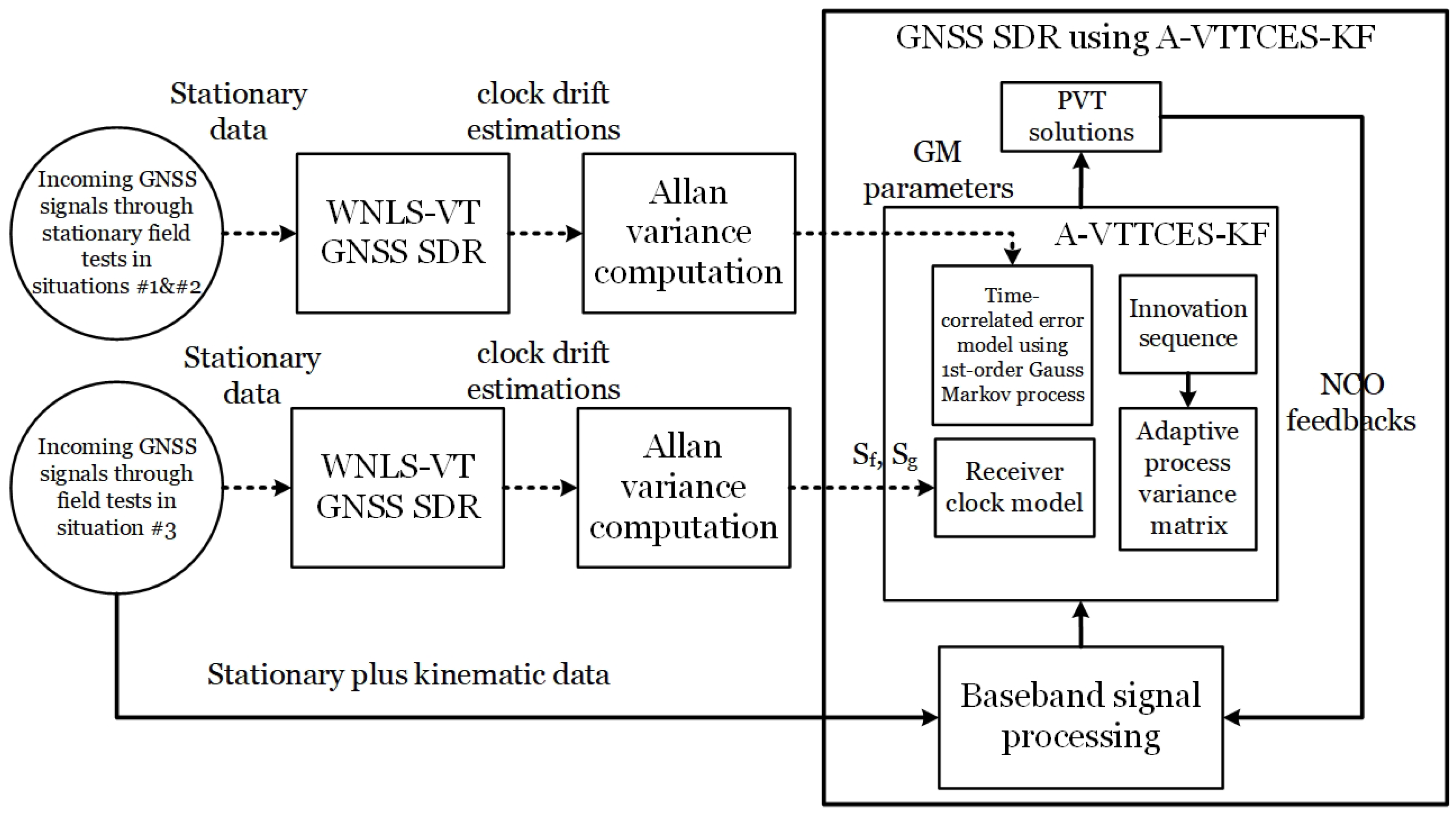
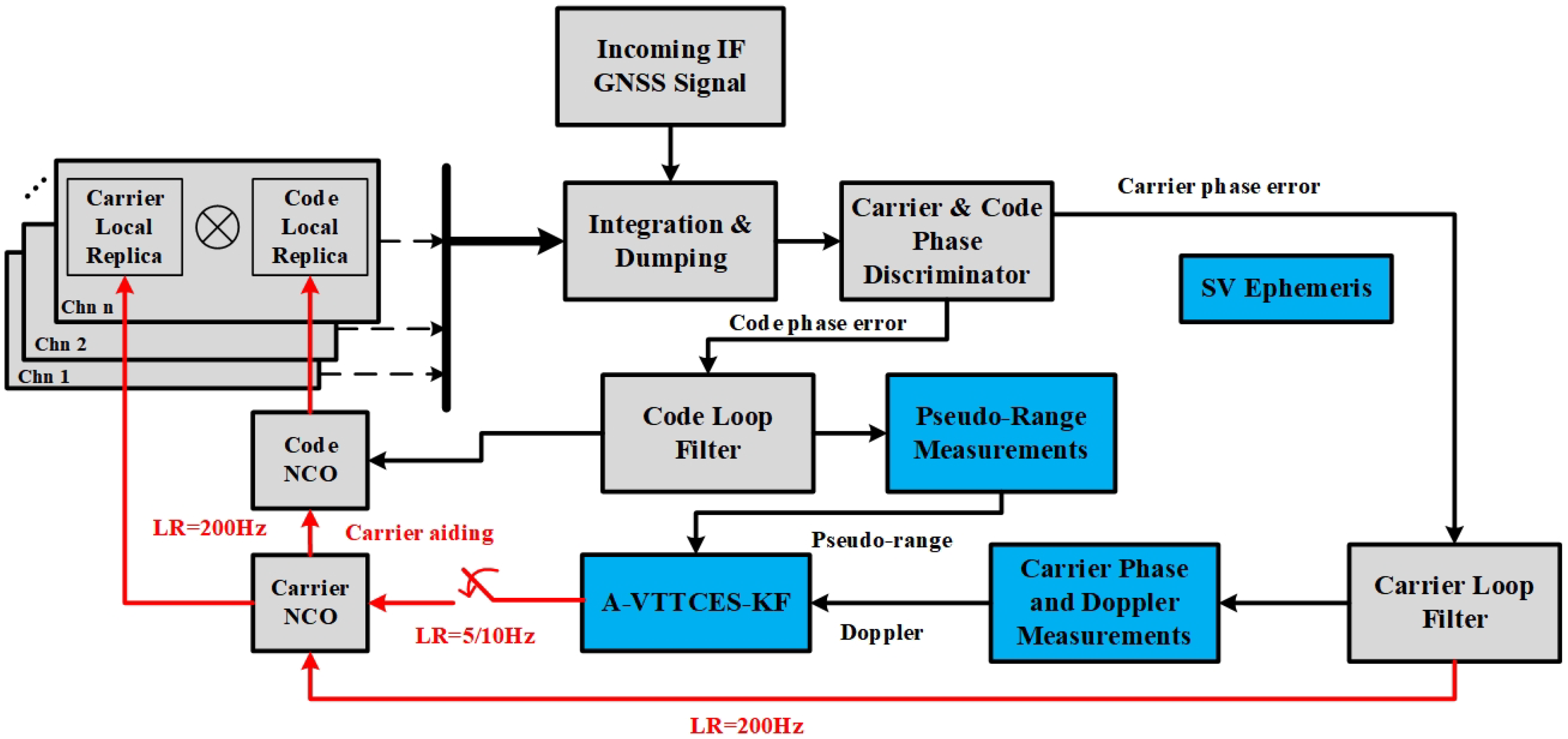
The setup for the field test based on the proposed A-VTTCES-KF is unchanged with the one for the stationary tests using the WNLS as illustrated in Figure 2. Furthermore, the corresponding parameter definitions for the GNSS SDR in the experiment are listed in

Table 4. Parameter settings of the GNSS SDR for the combined kinematic and static field test.

Parameters	Values
System and frequency	GPS L1 C/A
IF sampling rate	10.125 MHz
Coherent integration time	5 ms
VT LR	5/10/20 Hz
ST LR	200 Hz
Bandwidth of 3rd-order PLL for ST	18 Hz
Bandwidth of 3rd-order PLL for VT	5 Hz
Discriminator for code phase error	Noncoherent-early-minus-late-power discriminator
Discriminator for carrier phase error	Costas two-quadrant arctangent discriminator
Early-late spacing of code discriminator	0.2 chips
Re-acquisition algorithm	Not used

.

Both the carrier-phase-based real-time kinematic (RTK) positioning solutions and pseudo-range-based differential global positioning system (DGPS) solutions will be produced using the open-source package program, RTKLIB [77]. The related parameter settings for the RTK positioning algorithms are provided in

Table 5. Parameter settings for RTK positioning using the open-source package program of RTKLIB [77].

Parameters	Values	Descriptions
Positioning mode	Kinematic	Carrier-phase-based kinematic positioning
Integer ambiguity resolution	Continuous	Continuously static integer ambiguities are estimated and resolved
Min ratio to fix ambiguity	1.5	Set the integer ambiguity validation threshold for the ratio test; the test is related to the ratio of squared residuals of the best integer vector to the second-best vector
System and frequency	GPS L1 C/A	Single frequency positioning
Ionosphere correction	Broadcast	Apply broadcast ionospheric model
Troposphere correction	Saastamoinen	Apply Saastamoinen model
Satellite Ephemeris/Clock	Broadcast	Use broadcast ephemeris
Elevation mask	10 degrees	Set elevation mask angle in degree
Estimator mode	Post-processing	Forward filter solution

. Moreover, a short baseline which is far less than 20 kilometers is used in the field tests.

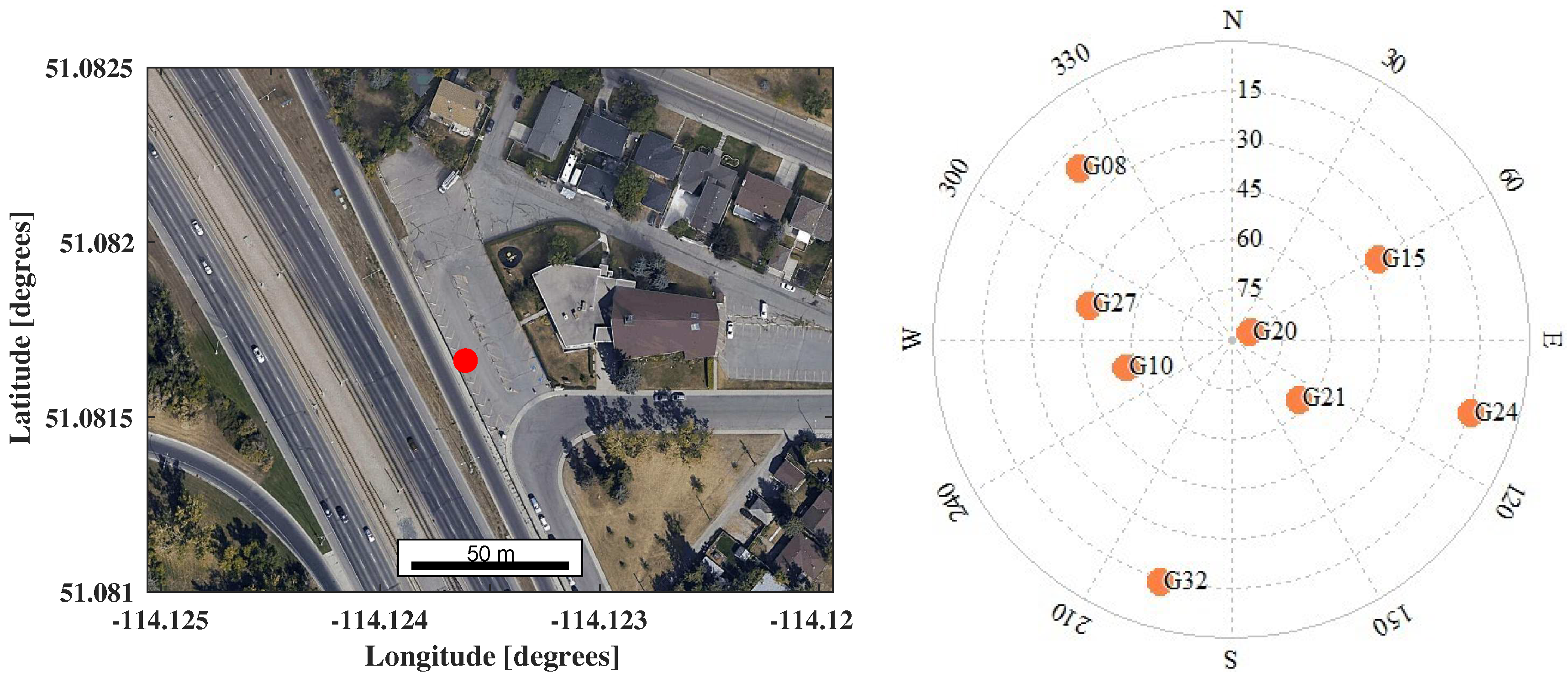
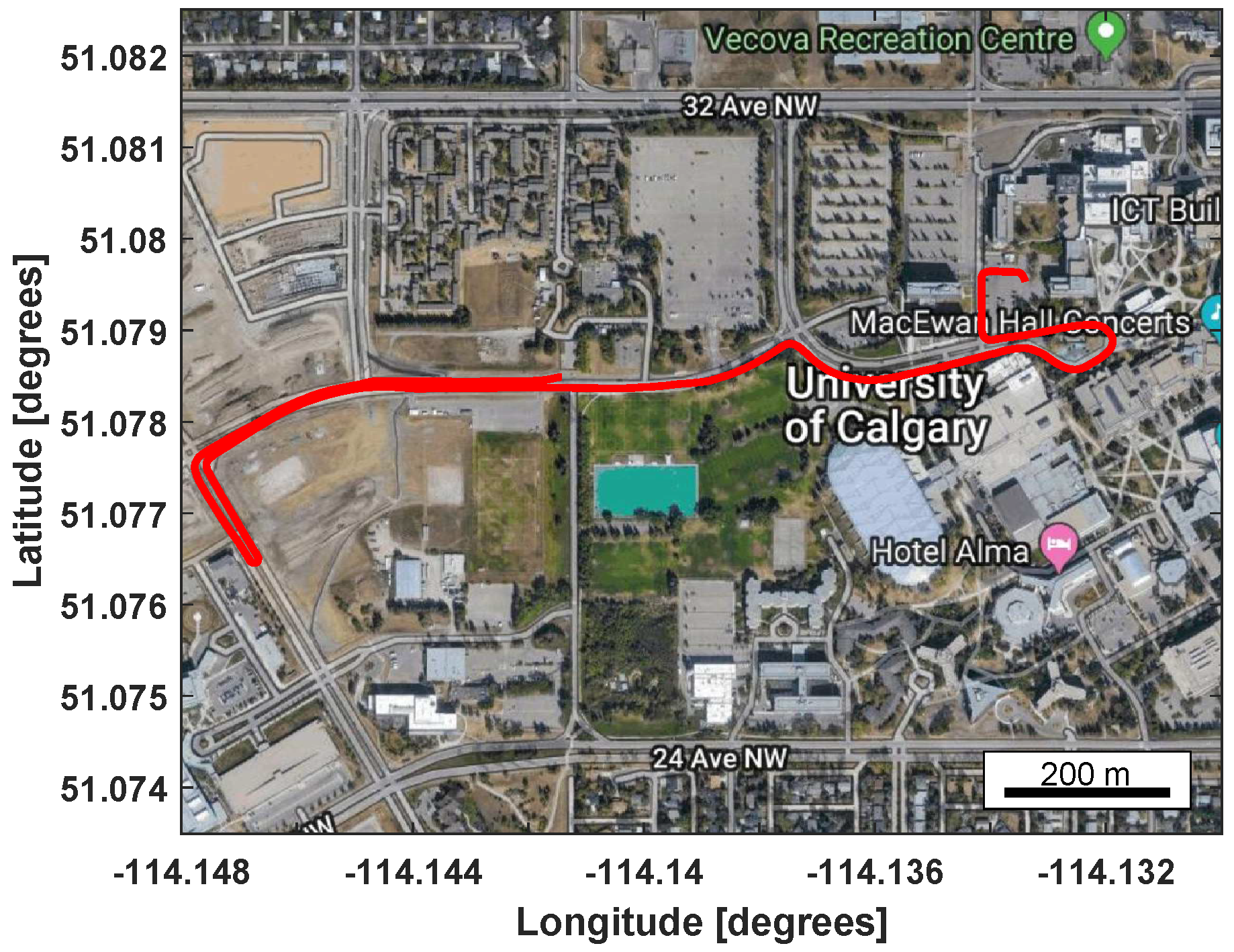
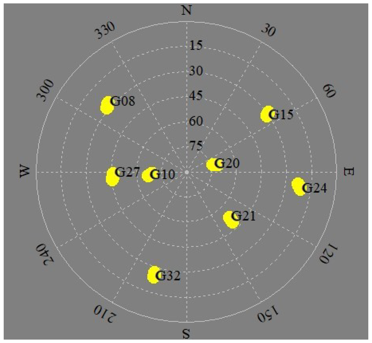
As shown in Figure 10, the trajectory is illustrated, and it is provided by the reference receiver of Trimble R10 in our work. Figure 11 demonstrates the view of the sky plot for all the contributed GPS SVs in the experiment and eight satellites are included.

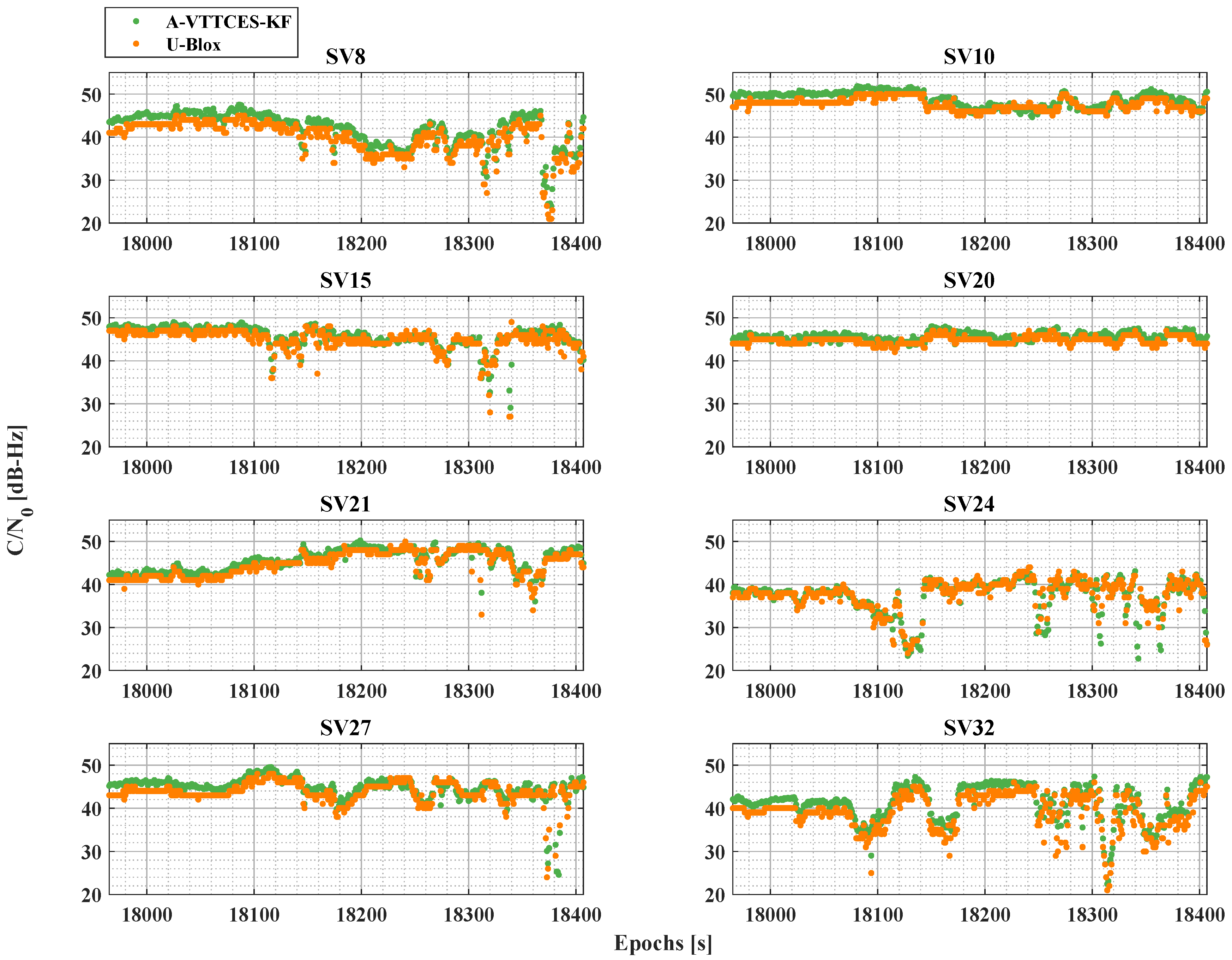
The trends of the signal power for all the tracking channels within the testing duration are provided in Figure 12 where U-Blox represents the estimations produced by the low-cost commercial U-Blox receiver. The SV10, SV20 maintain stable $C/N_0$ levels during the test due to the fact that they are embraced with the very high elevation angles. As to the other SVs from which the incoming GNSS signals are sometimes accidentally masked by the obstructions, e.g., the foliage and buildings during the whole testing. Furthermore, the received signals related to SV8, SV24, and SV32 are more frequently reduced by the environmental interference and blockage when compared with other signals, but the signal power can still be close to the level of the commercial U-Blox receiver in which the re-acquisition algorithm must be applied to confirm a high competition ability in the fierce commercial markets. It implies that the tracking performance of the GNSS receiver can highly be improved with the VT technique.

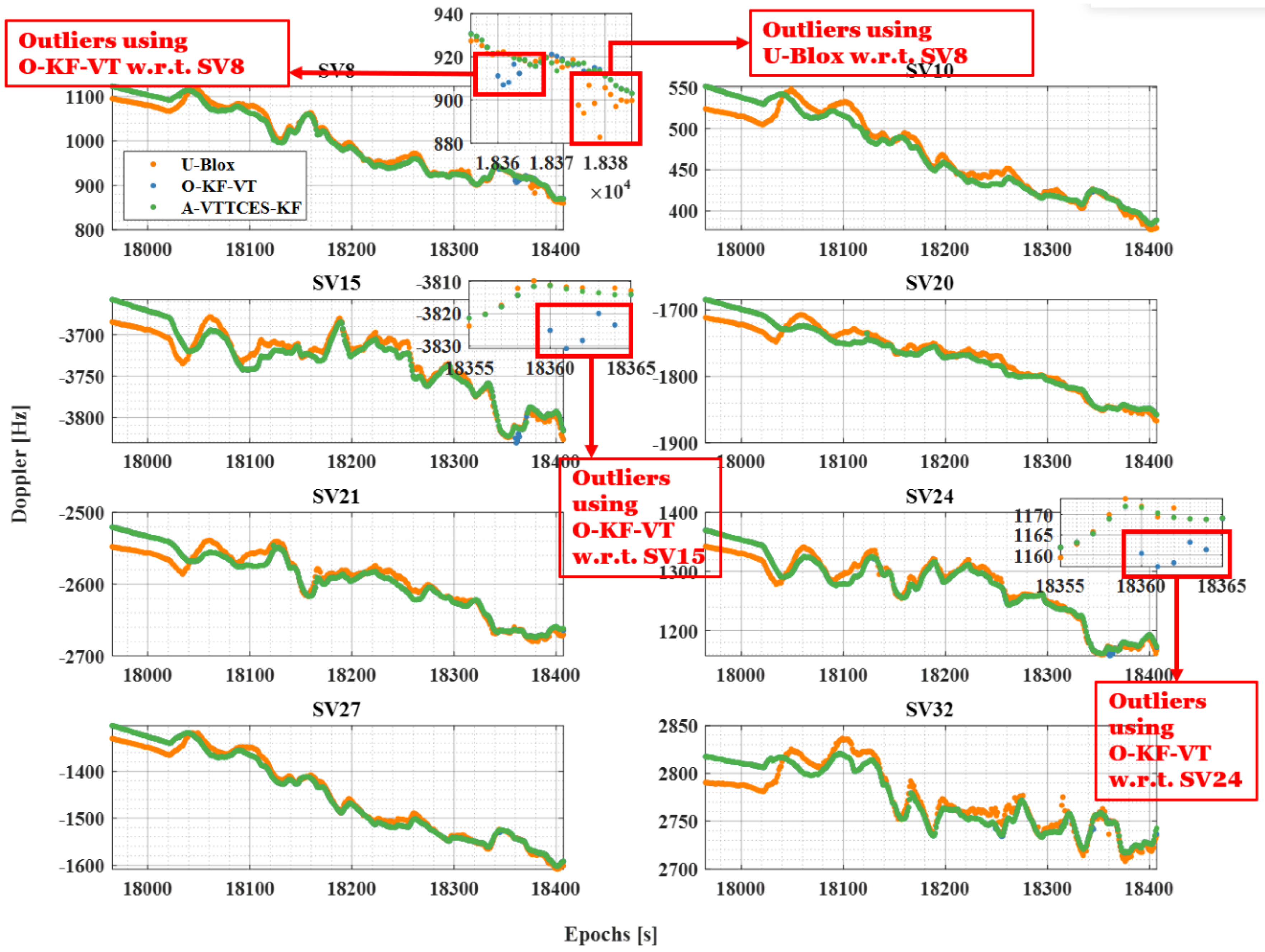
The Doppler estimation curves for all the used SVs are plot in Figure 13, where O-KF-VT denotes the estimations based on VT-based SDR using the ordinary adaptive KF algorithm regardless of compensating the time-correlated error. During the beginning dozens of seconds, there is a fixed bias Doppler error between the VT-based GNSS SDR and the U-Blox receiver in terms of all the satellites, since it takes some time for the KF to converge. When the convergence procedure is done, the Doppler measurement value of which the quality is highly dependent on the accuracy of the clock drift estimation can be gradually close to the values produced by the U-Blox receiver as far as possible. According to the zoomed-in pictures which is displayed in Figure 13, related to SV8, SV15, and SV24, the Doppler outliers are more possibly induced by the ordinary adaptive KF algorithm and the one provided by the U-Blox receiver, while the A-VTTCES-KF manages to maintain producing the Doppler measurements with the higher quality when compared with these two traditional approaches.

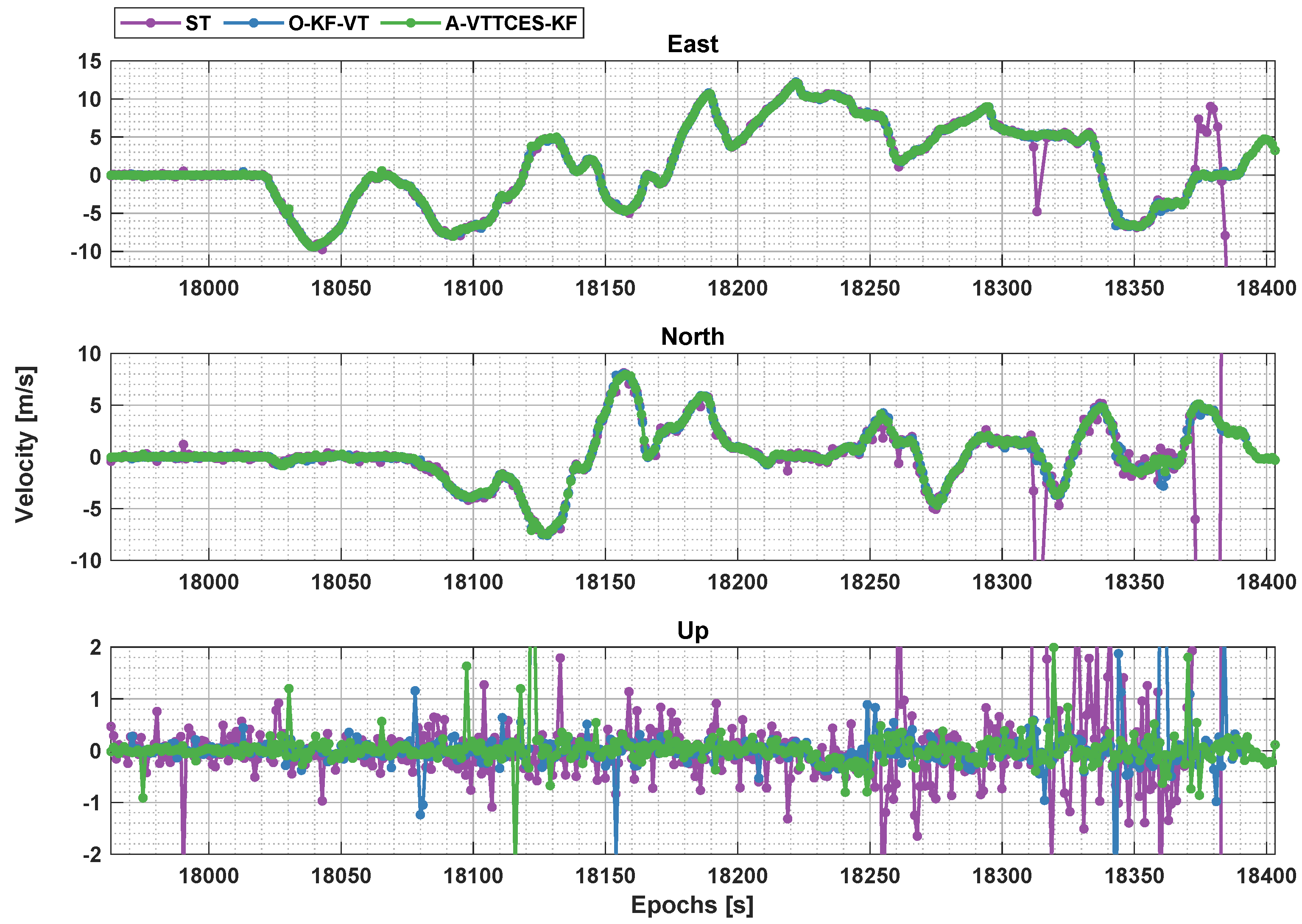
The velocity estimations through different algorithms are plot in Figure 14, where ST stands for the scalar tracking results of the GNSS SDR, and A-VTTCES-KF denotes the proposed algorithm as mentioned earlier. The tested ground vehicle was not moving at the first sixty seconds. After that, the autonomous vehicle started to move. The maximum absolute velocities in the east and north were approximately at 13 m/s and 9 m/s, respectively. The velocity estimation fails to be produced by the ST SDR after 18,370 s. Furthermore, it can also be found that there is a large estimation slip at around 18,310 s in the implementation process of the ST SDR.

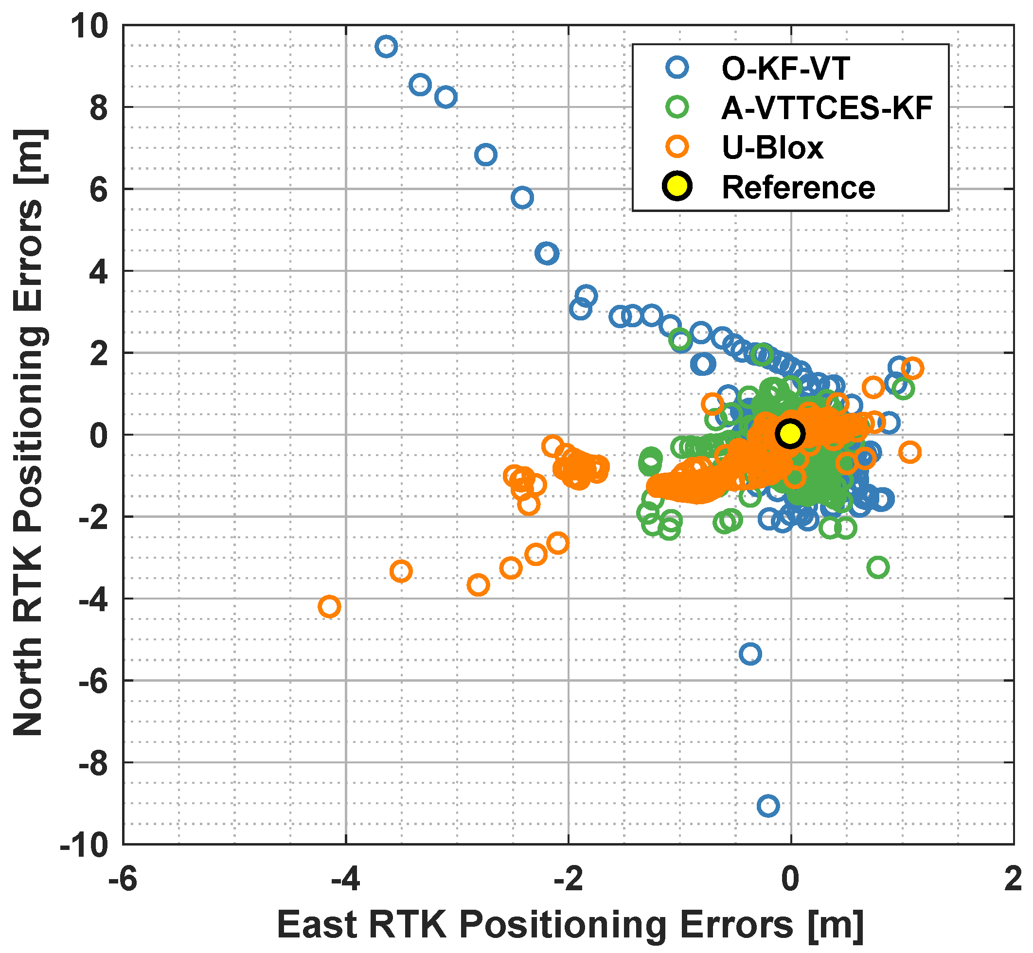
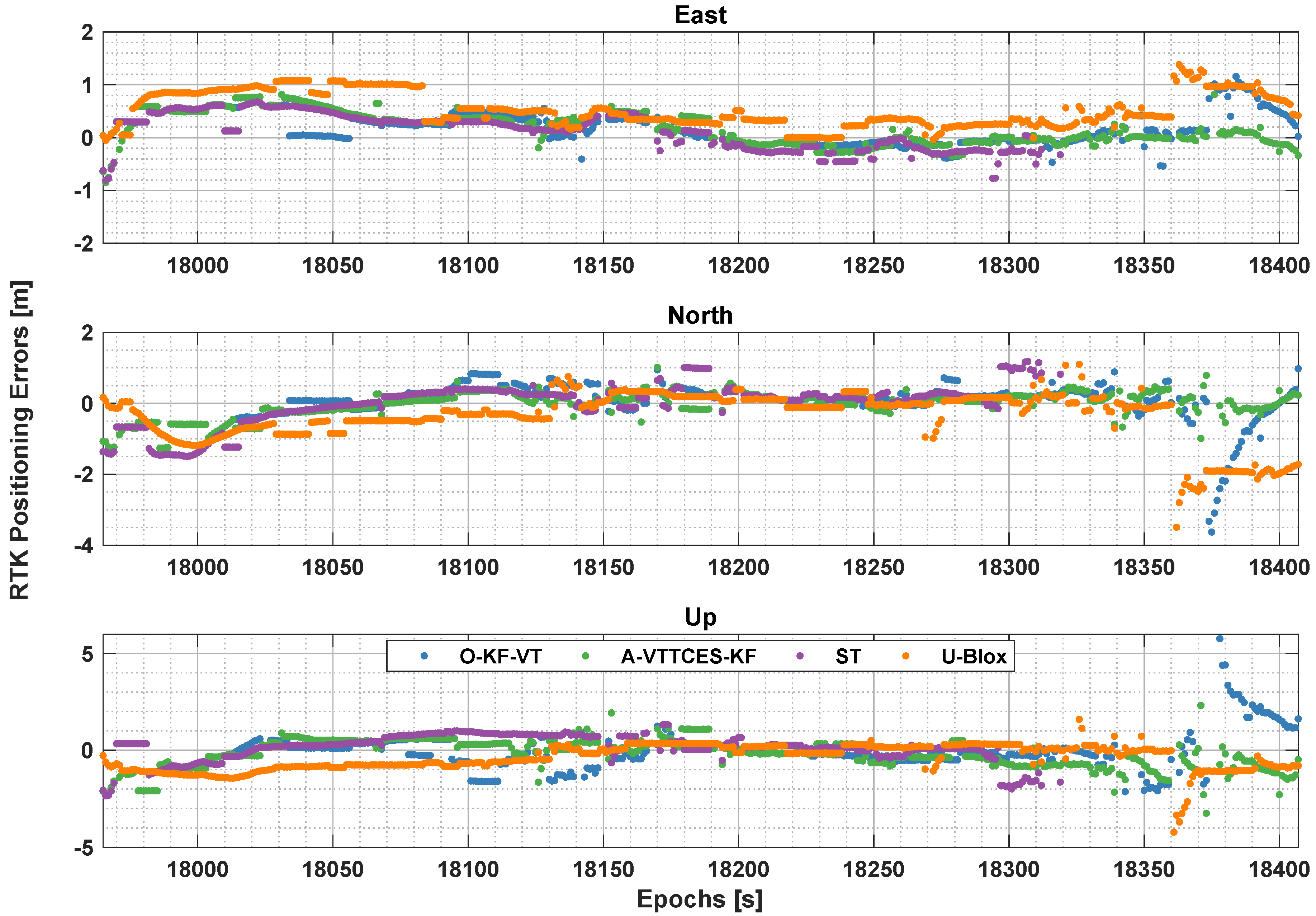
The error distributions produced by the RTK positioning method in the horizontal plain of the local level frame are illustrated in Figure 15. The error estimations output by the U-Blox receiver are also provided as the comparison. As shown in the figure, the number of the outliers are reduced by the proposed A-VTTCES-KF when compared with the ordinary KF algorithm.

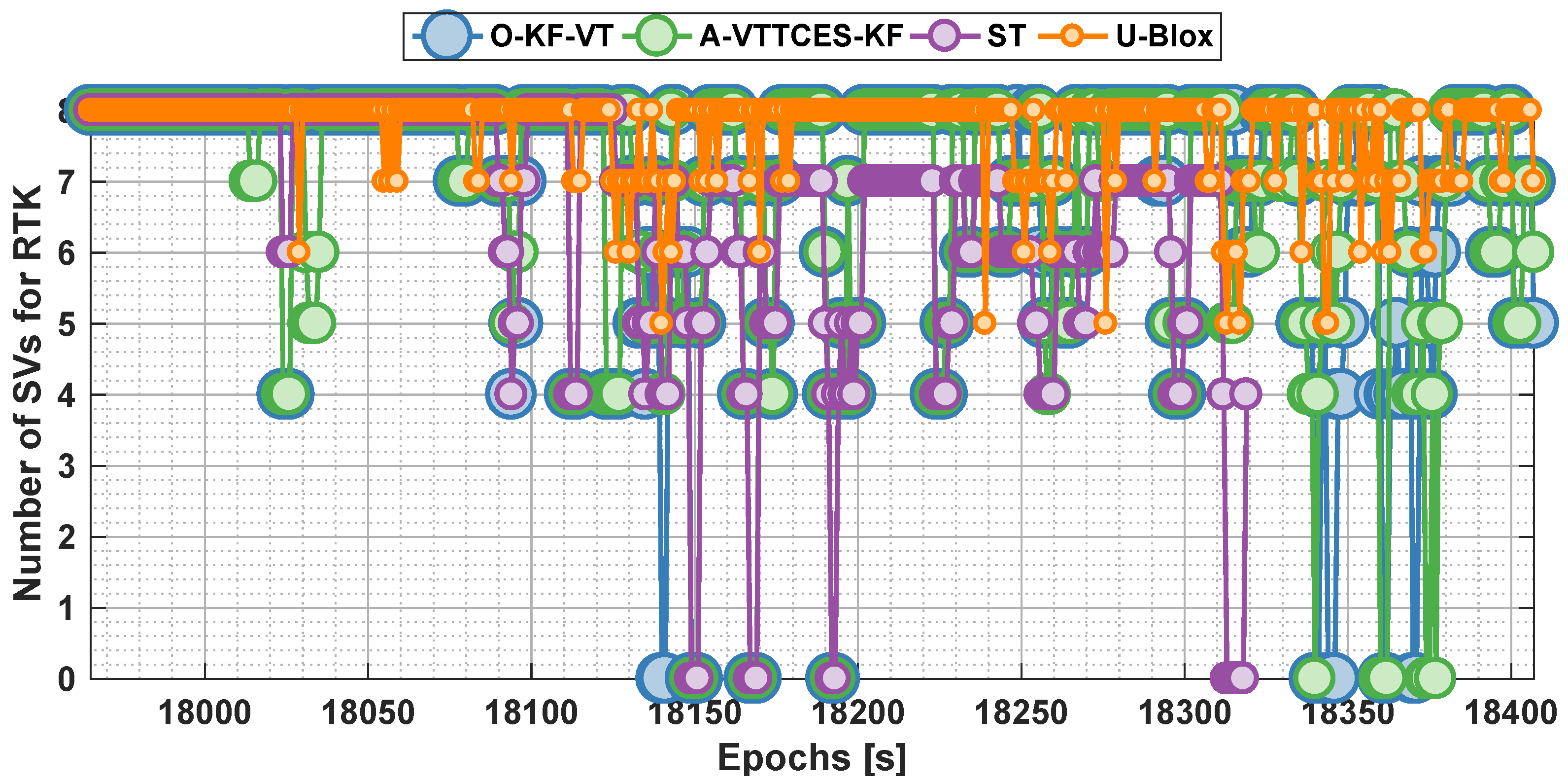
The curves in terms of how the number of satellites contributing to the PVT solutions changes with the spanning of the navigation epochs are displayed in Figure 16. Referring to Figure 12, apart from SV10 and SV20, the power loss of the other satellites occurred due to the blockages in the environmental place from the GPS time of 18,250 s to 18,350 s. The ST-based GNSS SDR failed to neither keep tracking most of the navigation satellites nor output the PVT solutions during and after this period. Nevertheless, the degraded numbers of satellites rise back again after some durations with severely environmental interferences in the VT GNSS SDR. On the other hand, although the SDR using the VT algorithms, i.e., O-KF-VT and A-VTTCES-KF, is not as robust as the commercial and self-contained U-Blox receiver, the tracking loops assisted with the VT technique are more than enough to tolerate the weak situation for much longer time when compared with the traditional scalar tracking architecture.

Since the field test is implemented in a moving autonomous ground vehicle, the dynamic stress residuals after the VT assistance on the tracking loop could be larger than the ones produced by a static receiver user. Hence, the bandwidth of the PLL is set to 5 Hz to make a trade-off between the tolerance in terms of the wide range of the dynamics caused by the moving vehicle and the reduction of the random noise through the PLL thermal noise jitter [42]. The 5 Hz is chosen as the value of the VT LR, by which to give a trade-off in decreasing the VT-induced time-correlated error and the dynamics-induced error residuals on the PLL. 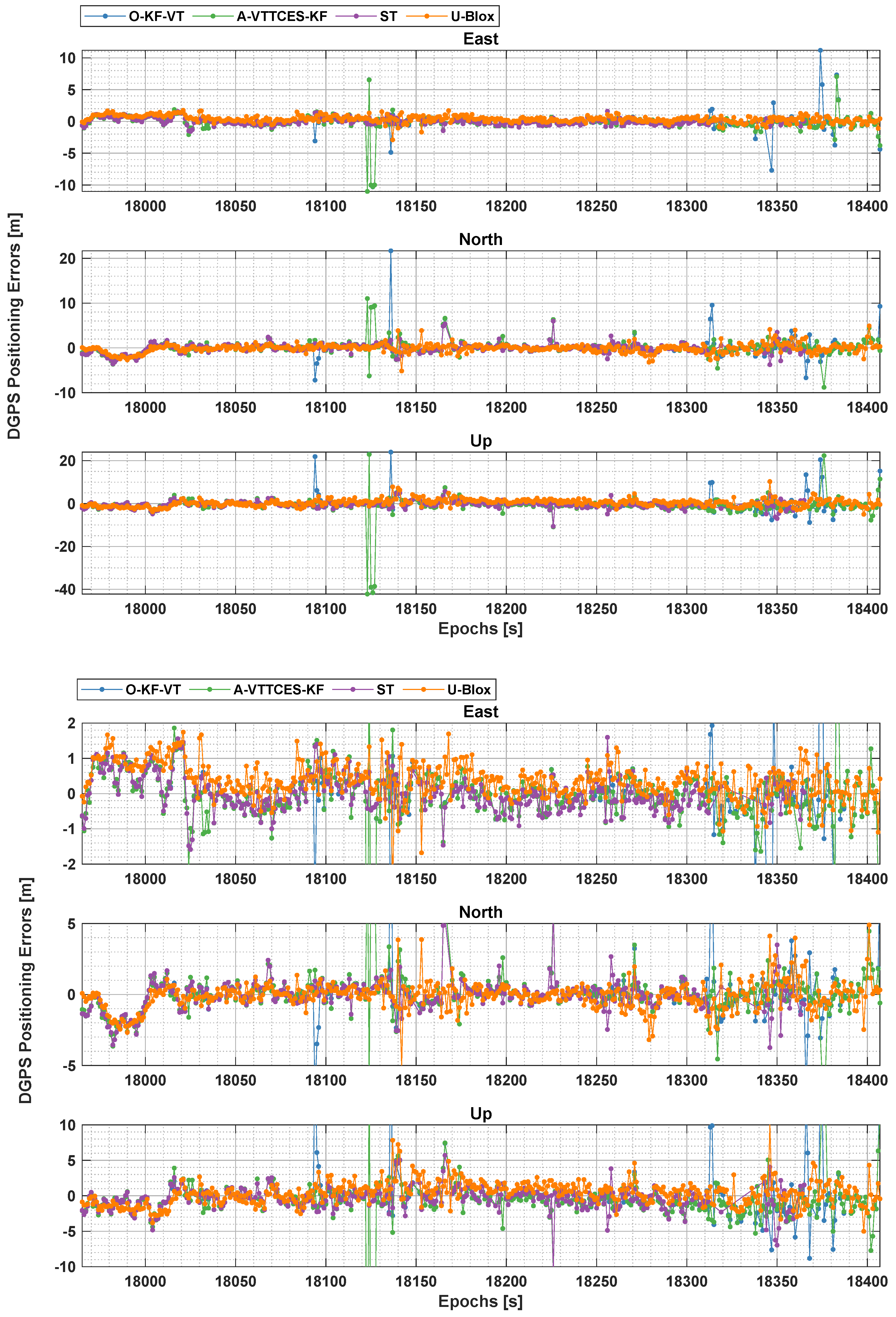Then, the results related to the RTK positioning errors are illustrated in Figure 17. The RTK positioning performance is determined with the quality of the carrier phase measurements. Besides, the results of the DGPS positioning error relying on the pseudo-range observations are also provided in Figure 18. The re-acquisition algorithms are not integrated in the GNSS SDR for our research as listed in Table 4. The continuous positioning solutions produced by the ST SDR are cut off at around 18,320 s and the receiver stops working from such time on, while the VT SDR as well as the U-Blox receiver can keep outputting the positioning results over the whole field test duration. Furthermore, the environmental condition is severe, the ordinary adaptive KF is possibly more sensitive to the weak power level and result in more outliers than the proposed A-VTTCES-KF. Some similarities, about which the positioning solutions are more likely to be biased in the weak and interfered environment, simultaneously occur between the GNSS SDR using the O-KF-VT algorithm and the U-Blox receiver as shown in Figure 17.

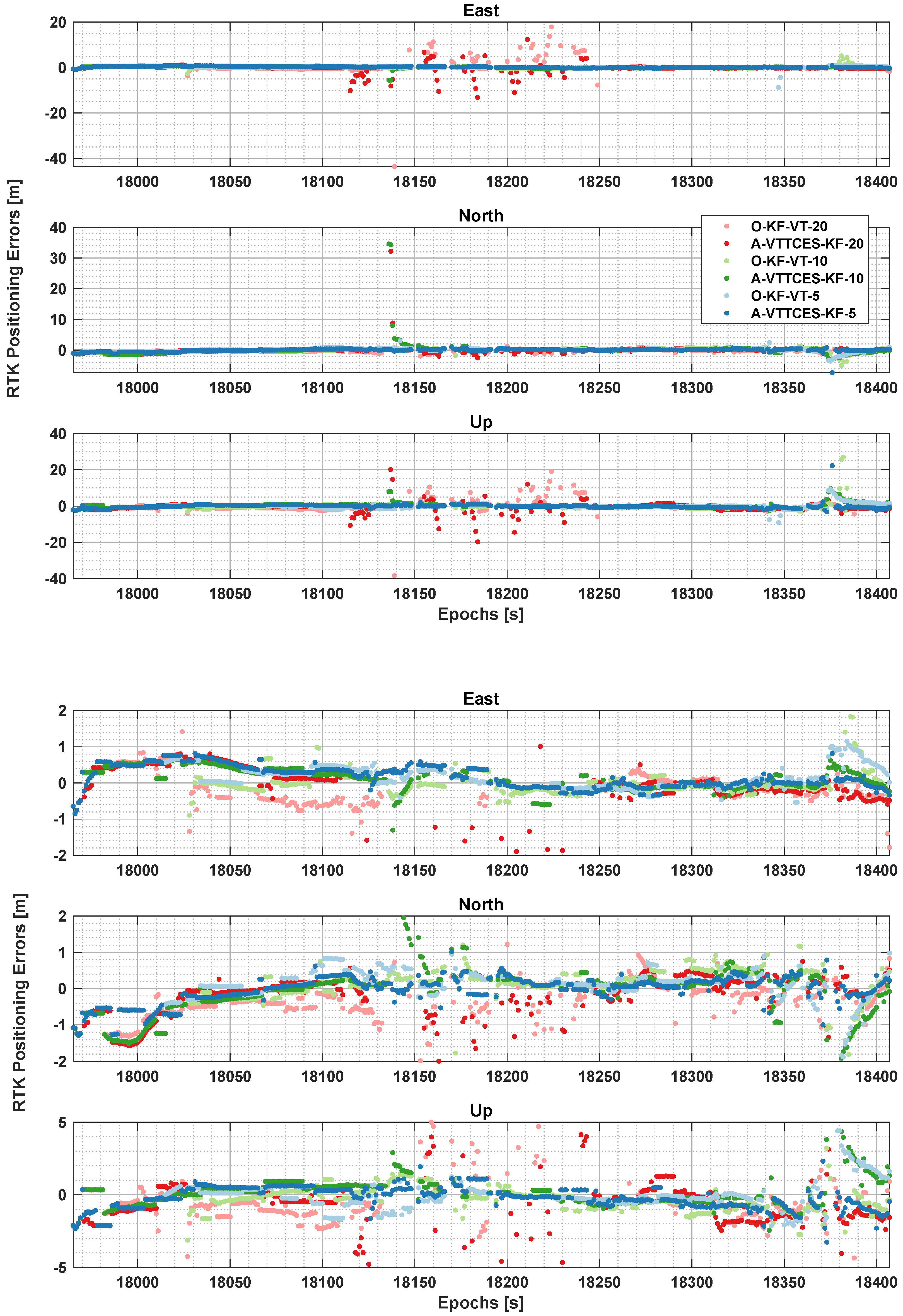
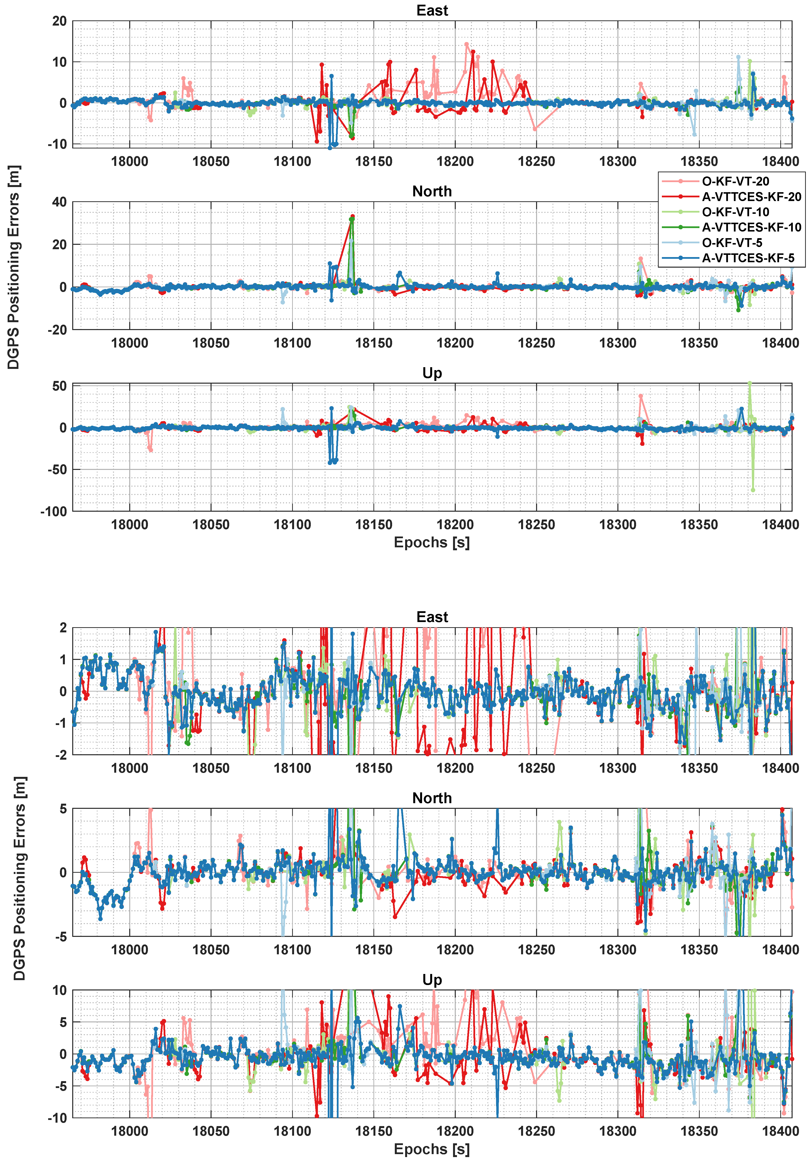
Both the A-VTTCES-KF and the O-KF-VT algorithms with different VT LRs, i.e., 5 Hz, 10 Hz, and 20 Hz, are also evaluated and compared using RTK and DGPS positioning algorithms. The results coming from the RTK methods are provided in Figure 19, while the ones associated with the DGPS approaches are depicted in Figure 20. When the VT LR increases to 20 Hz, the A-VTTCES-KF and the O-KF-VT architectures are proved to fail to provide the reliable positioning solutions during the period ranging from 18,110 s to 181,250 s. As shown in Figure 14, the resultant velocity exactly started to become larger at the epoch of 18,110 s. Hence, it can be verified that the value of 20 Hz generally exceeds the tolerance range of the VT LR, applied to the A-VTTCES-KF as well as the O-KF-VT, for a moving ground vehicle. A smaller value related to the VT LR in this work should be used and it is more reasonable to be applied in our proposed algorithms.

4. Discussion

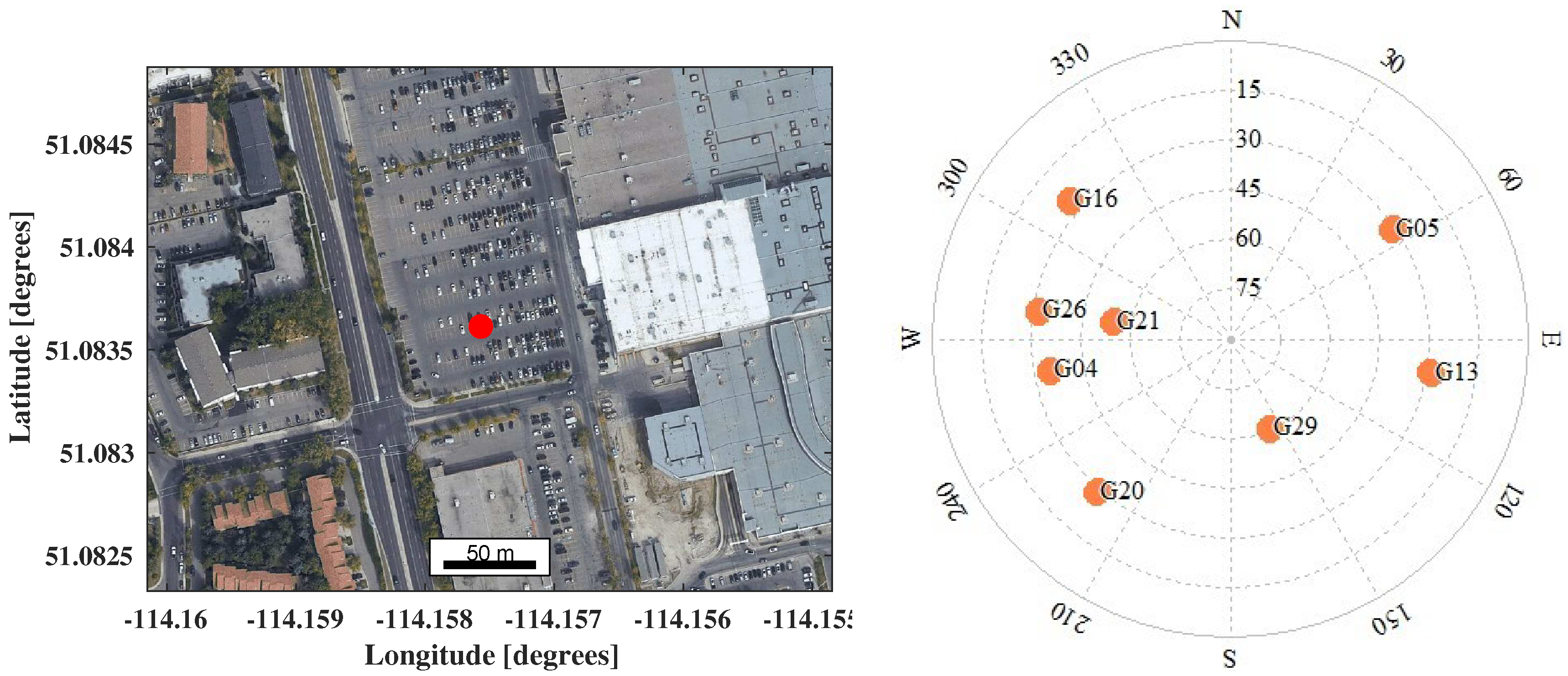
Maximum eight SVs contribute to the carrier-based and code-based positioning estimation processes for the GNSS SDR and the commercial U-Blox receiver in the field test in this work. The $C/N_0$ levels have been evaluated in the experiment, and the corresponding results are illustrated in Figure 12. With the assistance of the VT loop and the receiver velocity feedbacks, the tracking loop processing the satellite signal which are confronted with the signal masking problems can manage to tolerate the weak environment for a long time, e.g., the signals from SV8, SV24, and SV32. None of the acquired channels suffers from a signal loss in tracking procedure, and all the channels is being tracked through the whole time spanning of the field test in this work. It can be verified that, the proposed A-VTTCES-KF takes full advantages of the VT technique to help all the tracking channels, without the re-acquisition algorithm, keep working as what the self-contained commercial U-Blox receiver fulfills in a GNSS-challenged environment. Hence, the tracking robustness has been proved to be significantly improved by the A-VTTCES-KF technique.

Figure 13 depicts the Doppler estimation results. As mentioned before, the proposed algorithm can remove more unexpected blunders than the ordinary adaptive KF and the baseband signal processing method in the U-Blox receiver. The same conclusions can be drawn through the plots and results in Figure 15. In other words, it can be stated that the A-VTTCES-KF can provide more reliable Doppler observations. Also, the Doppler estimation, which the carrier NCO associated with the PLL updating accounts for, is made use of by the production of the pseudo-range measurement, such that the code-based observation quality is assured to be simultaneously enhanced through the proposed A-VTTCES-KF.

The velocities along the east, north, and up directions are illustrated in Figure 14, which indicates that the tested autonomous car is moving and kinematic. Such testing condition could be comparatively challenging and more than enough to verify the performance of the proposed algorithms in this research.

The self-designed GNSS SDR sometimes embraces less satellites for positioning than the U-Blox receiver as shown in Figure 16, but it does not mean that the tracking channels which do not participate in positioning perform worse than the counterparts in the U-Blox receiver. Since the GNSS SDR is less self-contained than the U-Blox receiver due to the discrepancy in terms of the entire design strategy. However, this work is not our contribution in the research, and the related information will be not involved with the subsequent discussions. Carrier-based and code-based positioning performances with different algorithms are compared in the experiments and the associated results are plot in Figure 17 and Figure 18, respectively. The positioning results depending on different VT LRs, i.e., 5 Hz, 10 Hz, and 20 Hz, are also computed during the post processing process, and the error curves with respect to the GPS time spanning are displayed in Figure 19 and Figure 20. Since the blunder positioning results could dramatically reduce the accuracy, and such ambiguous results with the contributions of the outliers cannot exactly reflect the real discrepancy among the proposed A-VTTCES-KF and the other ordinary methods. The three-sigma (3$\sigma$) rule is adopted to get rid of the unexpected and erroneous solutions, after which the remained positioning data series are subsequently exploited to obtain the corresponding root-mean-square errors (RMSEs). Assuming that the positioning errors follow the Gaussian white noise distribution, the 3$\sigma$ thresholds, which 99.7% of the absolute positioning errors should be no more than, can accordingly be approximately judged through the plot error curves from Figure 17 to Figure 20. The values in terms of the positioning RMSE are summarized and listed in

Table 6. RMSEs of the RTK and code-based DGPS positioning results.

PLL Bandwidth	VT LR	Positioning Method	3$\mathit{\sigma }$ Threshold [m]	Direction	O-KF-VT [m]	A-VTTCES-KF [m]	U-Blox [m]
5 Hz	5 Hz	RTK (3$\sigma$)	2	E	0.360	0.356	0.624
			2	N	0.461	0.365	0.674
			4	U	0.916	0.783	0.752
				All	1.087	0.934	1.187
		DGPS (3$\sigma$)	2	E	0.999	1.000	1.044
			5	N	0.980	0.926	0.914
			10	U	1.968	1.701	1.519
				All	2.415	2.180	2.057
5 Hz	10 Hz	RTK (3$\sigma$)	2	E	0.340	0.321	0.626
			2	N	0.569	0.605	0.672
			4	U	0.875	0.864	0.751
				All	1.098	1.103	1.186
		DGPS (3$\sigma$)	2	E	0.556	0.532	0.638
			5	N	1.071	1.009	0.970
			10	U	1.954	1.767	1.587
				All	2.297	2.103	1.966

, where E, N, U, and All represent the positioning errors along the east, north, up or vertical directions, and the resultant values through these three directions, respectively. Some states can be announced through the listed information which be subsequently discussed.

Firstly, the results on the condition that the VT LR is equal to 5 Hz will be discussed. As to the RTK positioning results, although positioning accuracies through both the O-KF-VT and the proposed A-VTTCES-KF in the vertical direction are faced with slight reductions, they have large improvements in the east and north directions compared with the solutions of the U-Blox receiver, as well as the resultant positioning results of these two algorithms are superior to the counterparts of the commercial receiver. In addition, the positioning performances produced by the A-VTTCES-KF exceeds the results obtained from the O-KF-VT in all directions. On the other hand, the O-KF-VT and A-VTTCES-KF positioning accuracies using the code-based DGPS algorithm are very close to each other in the east direction, while the latter performs better than the former in the east and up directions. In addition, the eastern DGPS positioning results produced by the VT-based SDR perform slightly better than the solutions estimated from the U-Blox receiver, while the positioning estimations along the other two directions using the SDR have a slightly worse performance.

Secondly, the positioning solutions using 10-Hz VT LR will be subsequently analyzed, and they will also be made comparisons with the ones produced by the VT-based SDR with the LR value of 5 Hz. The general results with respect to the RTK positioning using the A-VTTCES-KF show small reductions of the performance in the northern direction when compared with the O-KF-VT, but positioning accuracies are still gained in other two directions. Besides, the eastern and northern solutions produced by the U-Blox receiver are obtained in a weaker quality than the VT GNSS SDR, while the up-direction results are inversely addressed better than the solutions computed with the algorithms based on such VT mode. With regard to the DGPS estimations, the positioning results using the A-VTTCES-KF SDR outperform the solutions offered by the O-KF-VT system towards all the axes in the local level frame. Furthermore, a similarity in terms of the DGPS positioning results between the 10-Hz-VT-LR SDR and the U-Blox receiver can be found, when compared with the previous discussions on the comparisons related to the 5-Hz-VT-LR SDR and the U-Blox one.

A summary for the improved performances using the A-VTTCES-KF technique is listed in

Table 7. Summary on the improvements of the positioning accuracy using the A-VTTCES-KF. The term of O-KF-VT in the table corresponds to the improvements in percentage, with respect to the A-VTTCED-KF positioning accuracy, versus the counterpart of the SDR using O-KF-VT algorithm; the term of U-Blox in the table corresponds to the improvements in percentage, with respect to the A-VTTCED-KF positioning accuracy, versus the counterpart of the U-Blox receiver. The sign of minus represents that the accuracy is reduced.

PLL Bandwidth	VT LR	Positioning Method	Direction	O-KF-VT (%)	U-Blox (%)
5 Hz	5 Hz	RTK (3$\sigma$)	E	0.83	42.79
			N	21.26	46.14
			U	14.63	−3.99
			All	14.17	21.40
		DGPS (3$\sigma$)	E	−0.10	4.21
			N	5.51	−1.31
			U	13.57	−11.98
			All	9.73	−5.98
5 Hz	10 Hz	RTK (3$\sigma$)	E	5.59	48.72
			N	−6.33	9.97
			U	1.26	−15.05
			All	−0.46	7.00
		DGPS (3$\sigma$)	E	4.32	16.61
			N	5.79	−4.02
			U	9.57	−11.34
			All	8.45	−6.97

, where O-KF-VT in this table corresponds to the improvement percentages when the proposed algorithm is in comparison with the O-KF-VT algorithm; U-Blox denotes the counterparts with respect to the algorithm implemented by the U-Blox receiver. Some conclusions can be drawn through the results in this table.

Regarding the case using 5-Hz-VT-LR SDR, some discussions can be stated as follow.

Firstly, the A-VTTCES-KF outperforms the O-KF-VT in terms of the listed positioning results for most of the cases. Hence, the proposed algorithm can be confirmed that it is efficient on the error suppression. For example, the overall RTK positioning performance has been improved by 14.17%, while the positioning accuracy of the DGPS algorithm has a gain of 9.73%.

Secondly, the A-VTTCES-KF has a more distinctive superiority towards the north and up directions, while there are few accuracy improvements in the eastern axis. Some analysis will be subsequently given to explain the phenomenas. As mentioned earlier, the time-correlated error induced by the VT technique is tightly coupled with the clock drift estimations which are highly associated with the constitution of the Doppler measurements. Paying attention to the sky plot of the satellites in the kinematic field test as illustrated in Figure 11, more SVs are distributed along the east-west direction. As we know, the position accuracy is dependent on the dilution of precision (DOP) corresponding to the expression, ${\left({\mathbf{H}}^T\mathbf{H}\right)}^{-1}$, where $\mathbf{H}$ denotes the measurement design matrix [42]. This fact leads to the consequence that the clock drift residuals will be averaged along the east direction in the positioning estimation. Referring to Figure 11 and Figure 12, the signal power of SV32, which is shown to be significant of guaranteeing an adequate DOP distribution along the south-north direction, is severely reduced by the environmental interference at most of the time in the field test. Such that the positioning accuracies, especially related to the carrier-based positioning algorithms, will be highly degraded in terms of the northern direction. Because the clock drift errors are intimately added to the northern positioning results. As far as we know, the positioning accuracy in terms of the up direction is always highly influenced by the clock estimation results, since there must be no satellite distributed on or under the ground. This fact will not only decrease the positioning accuracy, but also tie the performance of the clock errors tightly to the positioning solutions, in terms of the height. Again, the time-correlated error coupled in the clock drift estimations could be suppressed by the proposed A-VTTCES-KF, so, the northern and vertical carrier-based positioning results, which have a close relationship with the clock drift noise error as explained earlier, will gain more distinctive improvements, when compared with the ones in terms of the eastern positioning results. The theoretical analysis has been proved to be consistent with the experimental results as listed in Table 7.

Thirdly, it can also be found that, the code-based DGPS positioning results, though, embrace similar improvement trends as the RTK solutions do, the increasing rates are smaller than the ones obtained from the RTK algorithm. As we know, the code-based positioning results are more likely to be relied on the clock bias estimations, and the carrier-based ones are more possibly dependent on the clock drift estimations. The clock bias can be assumed to be equivalent to the integration of the clock drift, and the integration time is identical to the update interval of the positioning estimation process. In other words, the clock drift passing through a resembling low-pass filter produced by the integration implementation gives the clock bias, and the time-correlated error will be reduced through this process. Therefore, it is reasonable that the DGPS positioning results have a slower improvement rate when compared with the RTK method.

Fourthly, there are significant increases in RTK positioning accuracy along the east and north directions when compared with the solutions produced by the U-Blox receiver, while a slight decrease in vertical accuracy occurs. The bandwidth of the PLL becomes smaller on the condition that a VT loop is involved in the GNSS SDR. For example, the bandwidth of the PLL applied to the ST loop is set to 18 Hz while the bandwidth with respect to the VT loop shrink to 5 Hz for our GNSS SDR in this research. The RTK solutions are more sensitive to the performance of the PLL and the estimation accuracy of the local clock drift due to the characteristics of the receiver design [42]. The vertical positioning results are ultra-tightly coupled with clock error estimations due to the geometry of the satellite distribution in the vertical direction. There is no sign transition in terms of the cosine direction vector for the height, while the corresponding coefficient for the clock error estimation is equivalent to one. In this case, this fact leads to the consequence that the height positioning results are highly related to the clock error estimations. Other two directions’ positioning results do not meet the same issue as the vertical one does. It can be inferred that the clock estimation in our presented GNSS SDR is less accurate than the results computed with the U-Blox receiver. Hence, it is totally possible that the local clock in the GNSS SDR is too coarse to enhance the positioning performance in the height.

Fifthly, the code-based DGPS positioning performance is not only relying on the PLL, but also mostly determined by the DLL, multipath mitigation algorithms applied in the code discriminator, and the clock bias estimations. The commercial U-Blox receiver can be assured to exploit some advanced techniques inside the GNSS receiver design to confirm the pseudo-range measurement to maintain a relatively high quality. Still, the way to improve the performance of the pseudo-range observation is not the primary contribution in this work. Therefore, it is acceptable that the positioning results based on the DGPS algorithms can be addressed better using the U-Blox receiver than the SDR with the A-VTTCES-KF in the north and vertical directions.

Regarding the comparisons in terms of the GNSS SDR using 10-Hz-VT-LR and 5-Hz-VT-LR algorithms, some conclusions can be subsequently drawn.

Sixthly, it can be found that the positioning accuracies in the north and vertical directions for both RTK and DGPS algorithms decline when using 10-Hz-VT-LR GNSS SDR. Accordingly, we can infer that when the VT LR increases, it will be harder to get rid of the time-correlated error in the VT loop through the proposed algorithm.

Finally, the eastern positioning accuracy are generally enhanced when the VT LR increases. For example, when compared with the O-KF-VT, the improved percentage of the RTK and DGPS with the 5-Hz VT LR is 0.83% and −0.10%, while the one with the 10-Hz VT LR is 5.59% and 4.32%, respectively.

5. Conclusions

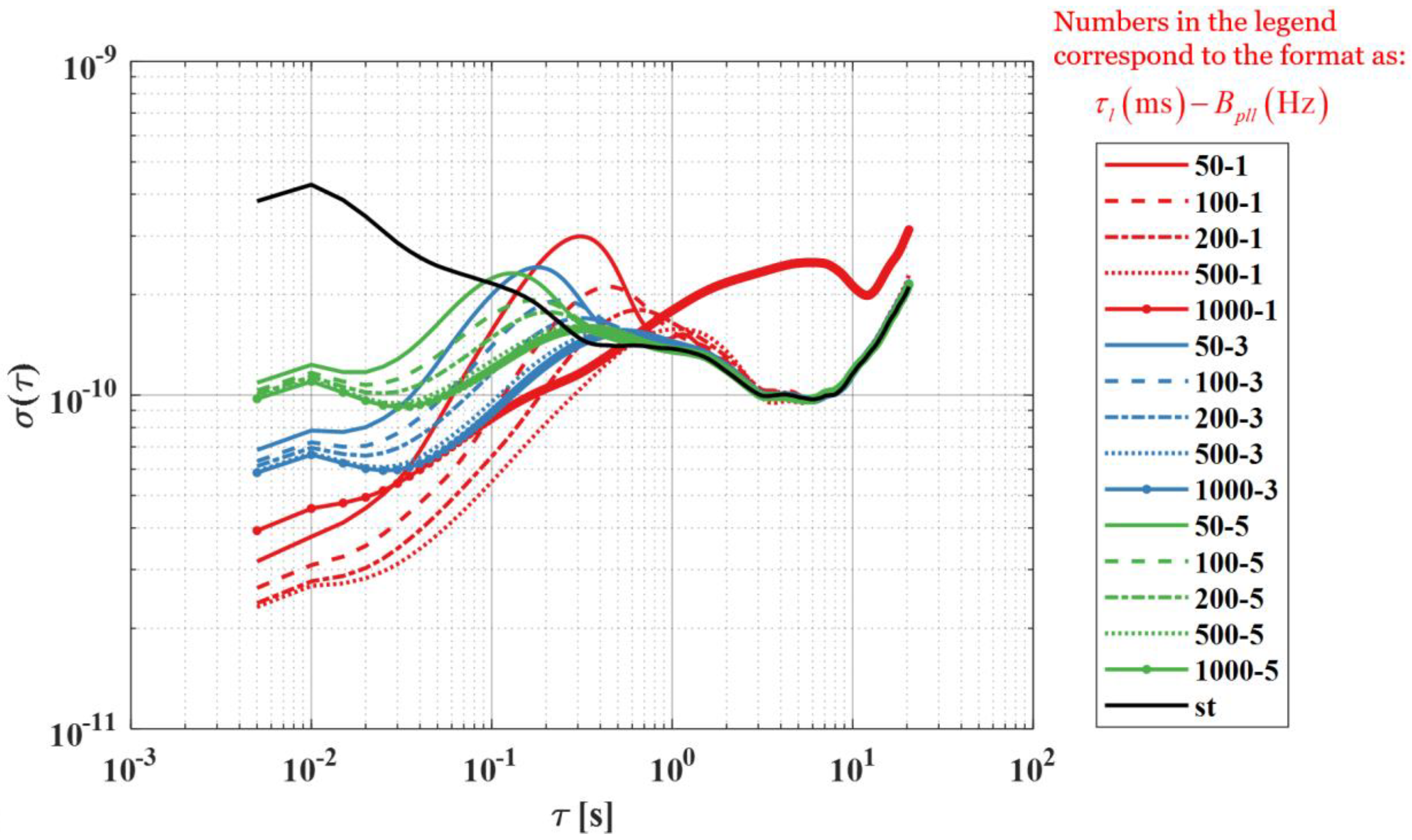
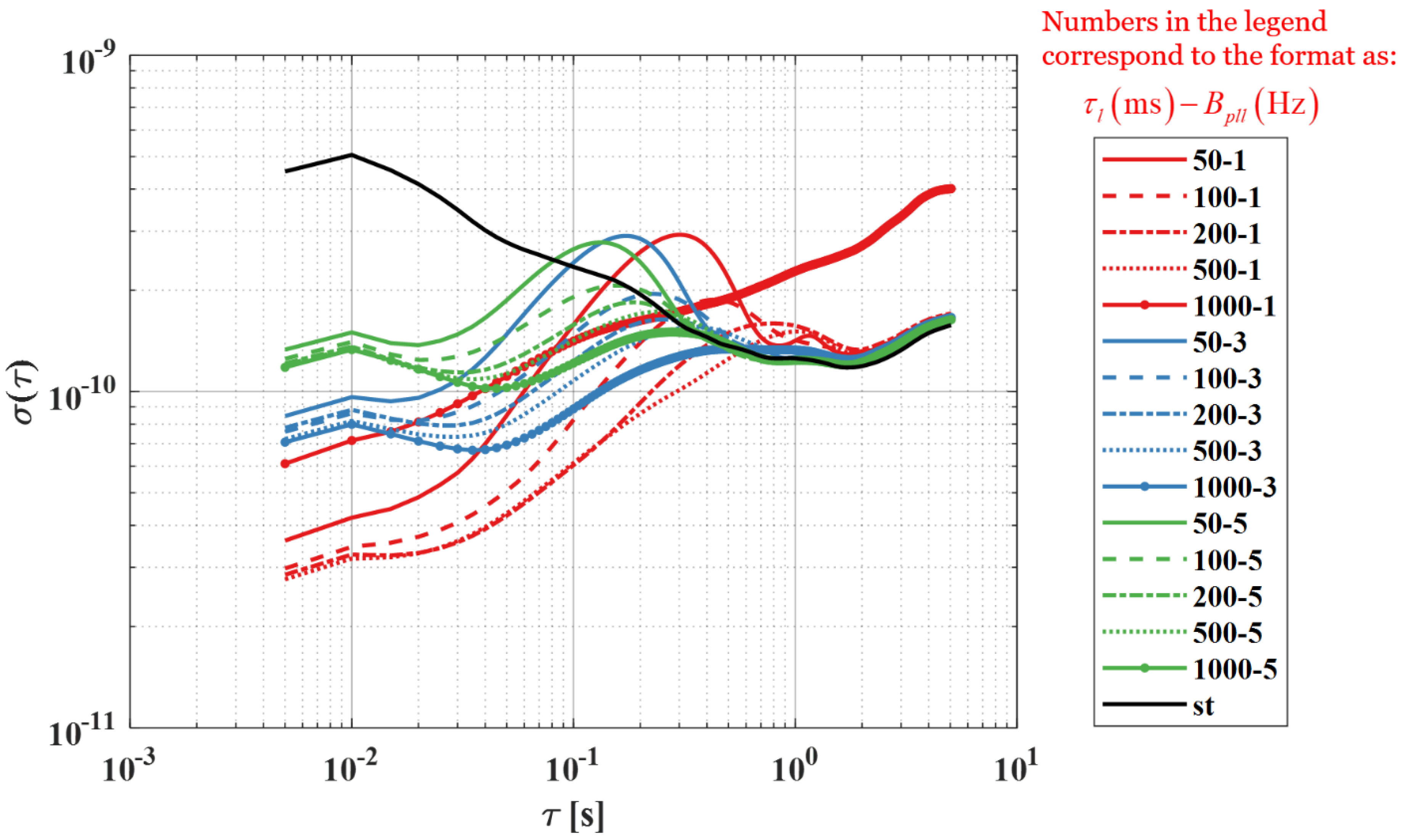
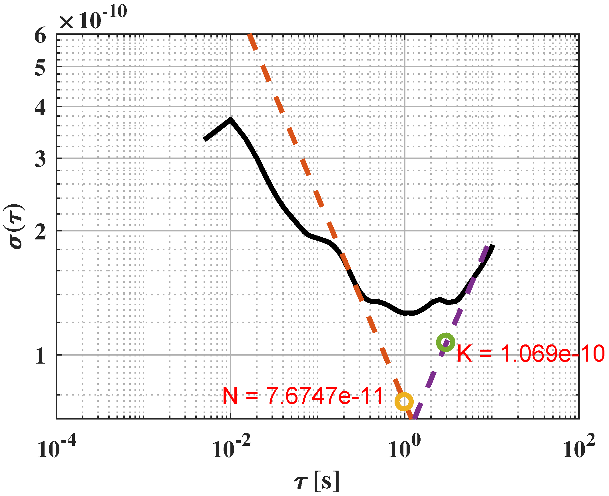
In this paper we provide an introduction about how to use the Allan variance algorithm to model the time-correlated error present in the local clock estimation data due to the VT feedback process. We applied the preliminary stationary field tests in two open-sky situations, and the estimated clock drift residual curves in terms of the Allan deviation are plot based on these static statistic data. A distinctive segment has been discovered in the curve shape related to the VT loop which can be differentiated from the one produced by the ST loop. The separate segment marks that the Markov noise is present in the clock drift estimated from the GNSS SDR using the VT technique instead of the ST architecture. In this work, the 1st-order Gauss-Markov process is adopted to model such noise source. Then, an improved A-VTTCES-KF algorithm is proposed to suppress the biased error in the PVT solutions caused by such VT-induced time-correlated error in the tracking loop. The state vector and the process covariance matrix can be improved with the given time-correlated model. Once the time-correlated error is estimated through the A-VTTCES-KF, the performance of the clock drift estimations can be enhanced by removing the known error source. In other words, the carrier NCO updates, i.e., Equation (24), can end up with obtaining a more accurate value, and the code NCO updates, which are aided by the carrier NCO, will accordingly be improved as well.

A Matlab-based GNSS SDR designed by the author is used to process the GPS L1 C/A signals in the field test to verify the proposed algorithms. The respective SDR using ordinary adaptive KF algorithm and the commercial low-cost U-Blox receiver are used for calculating the positioning solutions, relied on an open-source package program, RTKLIB, as the comparisons. The coherent integration time is chosen as 5 ms in this work, so the loop rate of the PLL and DLL updates is 200 Hz in the GNSS SDR. The experimental results have demonstrated that, when the LR of the VT architecture is set to 5 Hz, the GNSS SDR using the proposed A-VTTCES-KF can embrace the improvements of 14.17% and 21.40% in terms of the RTK positioning when compared with the VT SDR with the ordinary adaptive KF method and the U-Blox receiver, respectively. In addition, the DGPS positioning solutions produced by the proposed VT SDR also outperform the ones obtained from the SDR using the ordinary method method at a percentage of 9.73%. Towards the case of increasing the performance based on the code-based positioning algorithms, the receiver design methods, e.g., the discriminator applied for the code error estimation, the DLL bandwidth, could dramatically make a difference on the navigation solutions. Since the multipath interference has a higher influence on the pseudo-range measurement than the carrier phase measurement. Under this circumstance, it is acceptable that the DGPS positioning results estimated from the U-Blox receiver performed better than the proposed SDR architecture. It should also be noted that the proposed approach seems to work more efficiently in areas where the VT LR is lower. For example, the enhanced GNSS SDR was proved to provide higher improvements when the VT LR is chosen as 5Hz rather than the case of the VT LR being set to 10 Hz.

An approach using the Allan variance to account for the time-correlated error present in the typical VT loop has been proposed in this work, and the idea to compensate such error towards the VT-based receiver design has seldom been mentioned in previous researches. The time-correlated error would add extra biases to the GNSS measurements such that the code-based and carrier-phase-based positioning results can be intimately affected, and the related accuracies will be accordingly decreased. Under this circumstance, two major improvements have been made through the proposed A-VTTCES-KF. Firstly, the time-correlated error present in the measurements produced by the VT-based GNSS SDR can be reduced; secondly, the more accurate PVT results or state estimations in the prior epoch will be realized based on the first improvement, so that the innovation sequence used in the A-VTTCES-KF is able to adaptively enhance the performance of the priori process covariance matrix in the KF. It means that the positioning accuracy using the A-VTTCES-KF in the current epoch can be again increased. In a word, both bias in terms of the time-correlated error and the random noise error in terms of the KF process covariance matrix are promising to be suppressed by the proposed approach towards the VT loop architecture. These superiorities can overall improve the PVT performance produced by the VT-based GNSS receiver, as well as enhance its robustness ability in the challenging environments, e.g., weak, dynamic, or multipath-interfered cases. In our case, only the GM process is identified and quantified by the Allan deviation curve towards the time-correlated error modelling, but such error source may be accounted for using more than one models besides of the GM process in reality. An improved tool, GMWM, has recently been proposed to analyze the noise source distribution of the stochastic data [67]. Our research for the time-correlated error modelling in the VT loop may be further fulfilled in a more precision way with the GMWM in the future work.

References

1. Yang, T.; Ren, Q.; Zhang, F.; Xie, B.; Ren, H.; Li, J.; Zhang, Y. Hybrid Camera Array-Based UAV Auto-Landing on Moving UGV in GPS-Denied Environment. Remote Sens. 2018, 10, 1829. [Google Scholar] [CrossRef]
2. Sabet, M.T.; Daniali, H.M.; Fathi, A.; Alizadeh, E. Experimental analysis of a low-cost dead reckoning navigation system for a land vehicle using a robust AHRS. Robot. Auton. Syst. 2017, 95, 37–51. [Google Scholar] [CrossRef]
3. Sukkarieh, S.; Nebot, E.M.; Durrant-Whyte, H.F. A high integrity IMU/GPS navigation loop for autonomous land vehicle applications. IEEE Trans. Robot. Autom. 1999, 15, 572–578. [Google Scholar] [CrossRef]
4. Zhou, Z.; Wu, J.; Wang, J.; Fourati, H. Optimal, recursive and sub-optimal linear solutions to attitude determination from vector observations for GNSS/accelerometer/magnetometer orientation measurement. Remote Sens. 2018, 10, 377. [Google Scholar] [CrossRef]
5. Wang, X.; Wang, W. Nonlinear signal-correction observer and application to UAV navigation. IEEE Trans. Ind. Electron. 2019, 66, 4600–4607. [Google Scholar] [CrossRef]
6. Vetrella, A.R.; Causa, F.; Renga, A.; Fasano, G.; Accardo, D.; Grassi, M. Multi-UAV Carrier Phase Differential GPS and Vision-based Sensing for High Accuracy Attitude Estimation. J. Intell. Robot. Syst. 2019, 93, 245–260. [Google Scholar] [CrossRef]
7. Albetis, J.; Jacquin, A.; Goulard, M.; Poilvé, H.; Rousseau, J.; Clenet, H.; Dedieu, G.; Duthoit, S. On the Potentiality of UAV Multispectral Imagery to Detect Flavescence dorée and Grapevine Trunk Diseases. Remote Sens. 2019, 11, 23. [Google Scholar] [CrossRef]
8. Tamirat, T.W.; Pedersen, S.M.; Lind, K.M. Farm and operator characteristics affecting adoption of precision agriculture in Denmark and Germany. Acta Agric. Scand. Sect. B Soil Plant Sci. 2018, 68, 349–357. [Google Scholar] [CrossRef]
9. Guo, J.; Li, X.; Li, Z.; Hu, L.; Yang, G.; Zhao, C.; Fairbairn, D.; Watson, D.; Ge, M. Multi-GNSS precise point positioning for precision agriculture. Precis. Agric. 2018, 19, 895–911. [Google Scholar] [CrossRef]
10. Keskin, M.; Sekerli, Y.E.; Kahraman, S. Performance of two low-cost GPS receivers for ground speed measurement under varying speed conditions. Precis. Agric. 2017, 18, 264–277. [Google Scholar]
11. Bengochea-Guevara, J.; Conesa-Muñoz, J.; Andújar, D.; Ribeiro, A. Merge fuzzy visual servoing and GPS-based planning to obtain a proper navigation behavior for a small crop-inspection robot. Sensors 2016, 16, 276. [Google Scholar] [CrossRef]
12. Handscombe, J.; Yu, H.Q. Low-cost and data anonymised city traffic flow data collection to support intelligent traffic system. Sensors 2019, 19, 347. [Google Scholar] [CrossRef]
13. Huang, B.; Liu, W.; Wang, T.; Li, X.; Song, H.; Liu, A. Deployment Optimization of Data Centers in Vehicular Networks. IEEE Access 2019, 7, 20644–20663. [Google Scholar] [CrossRef]
14. Chen, C.; Jiao, S.; Zhang, S.; Liu, W.; Feng, L.; Wang, Y. TripImputor: Real-time imputing taxi trip purpose leveraging multi-sourced urban data. IEEE Trans. Intell. Transp. Syst. 2018, 19, 3292–3304. [Google Scholar] [CrossRef]
15. Lagkas, T.; Argyriou, V.; Bibi, S.; Sarigiannidis, P. UAV IoT Framework Views and Challenges: Towards Protecting Drones as “Things”. Sensors 2018, 18, 4015. [Google Scholar] [CrossRef] [PubMed]
16. Shila, D.M.; Srivastava, K. CASTRA: Seamless and Unobtrusive Authentication of Users to Diverse Mobile Services. IEEE Internet Things J. 2018, 5, 4042–4057. [Google Scholar] [CrossRef]
17. Li, Y.; He, Z.; Gao, Z.; Zhuang, Y.; Shi, C.; El-Sheimy, N. Towards Robust Crowdsourcing-Based Localization: A Fingerprinting Accuracy Indicator Enhanced Wireless/Magnetic/Inertial Integration Approach. IEEE Internet Things J. 2018. [Google Scholar] [CrossRef]
18. Egido, A.; Caparrini, M.; Ruffini, G.; Paloscia, S.; Santi, E.; Guerriero, L.; Pierdicca, N.; Floury, N. Global navigation satellite systems reflectometry as a remote sensing tool for agriculture. Remote Sens. 2012, 4, 2356–2372. [Google Scholar] [CrossRef]
19. Camps, A.; Vall·llossera, M.; Park, H.; Portal, G.; Rossato, L. Sensitivity of TDS-1 GNSS-R reflectivity to soil moisture: Global and regional differences and impact of different spatial scales. Remote Sens. 2018, 10, 1856. [Google Scholar] [CrossRef]
20. Carreno-Luengo, H.; Lowe, S.; Zuffada, C.; Esterhuizen, S.; Oveisgharan, S. Spaceborne GNSS-R from the SMAP mission: First assessment of polarimetric scatterometry over land and cryosphere. Remote Sens. 2017, 9, 362. [Google Scholar] [CrossRef]
21. Lin, W.; Portabella, M.; Foti, G.; Stoffelen, A.; Gommenginger, C.; He, Y. Toward the Generation of a Wind Geophysical Model Function for Spaceborne GNSS-R. IEEE Trans. Geosci. Remote Sens. 2018. [Google Scholar] [CrossRef]
22. Gleason, S. Towards sea ice remote sensing with space detected GPS signals: Demonstration of technical feasibility and initial consistency check using low resolution sea ice information. Remote Sens. 2010, 2, 2017–2039. [Google Scholar] [CrossRef]
23. Bussy-Virat, C.D.; Ruf, C.S.; Ridley, A.J. Relationship between temporal and spatial resolution for a constellation of GNSS-R satellites. IEEE J. Sel. Top. Appl. Earth Obs. Remote Sens. 2019, 12, 16–25. [Google Scholar] [CrossRef]
24. Carreno-Luengo, H.; Luzi, G.; Crosetto, M. Impact of the Elevation Angle on CYGNSS GNSS-R Bistatic Reflectivity as a Function of Effective Surface Roughness over Land Surfaces. Remote Sens. 2018, 10, 1749. [Google Scholar] [CrossRef]
25. Gao, Z.; Li, Y.; Zhuang, Y.; Yang, H.; Pan, Y.; Zhang, H. Robust Kalman Filter Aided GEO/IGSO/GPS Raw-PPP/INS Tight Integration. Sensors 2019, 19, 417. [Google Scholar] [CrossRef] [PubMed]
26. Liu, Z.; El-Sheimy, N.; Yu, C.; Qin, Y. Motion constraints and vanishing point aided land vehicle navigation. Micromachines 2018, 9, 249. [Google Scholar] [CrossRef] [PubMed]
27. Chiang, K.; Tsai, G.; Chang, H.; Joly, C.; EI-Sheimy, N. Seamless navigation and mapping using an INS/GNSS/grid-based SLAM semi-tightly coupled integration scheme. Inf. Fusion 2019, 50, 181–196. [Google Scholar] [CrossRef]
28. Li, T.; Zhang, H.; Gao, Z.; Niu, X.; El-sheimy, N. Tight Fusion of a Monocular Camera, MEMS-IMU, and Single-Frequency Multi-GNSS RTK for Precise Navigation in GNSS-Challenged Environments. Remote Sens. 2019, 11, 610. [Google Scholar] [CrossRef]
29. Vollrath, A.; Zucca, F.; Bekaert, D.; Bonforte, A.; Guglielmino, F.; Hooper, A.; Stramondo, S. Decomposing DInSAR time-series into 3-D in combination with GPS in the case of low strain rates: An application to the Hyblean Plateau, Sicily, Italy. Remote Sens. 2017, 9, 33. [Google Scholar] [CrossRef]
30. Palm, S.; Sommer, R.; Stilla, U. Mobile Radar Mapping–Subcentimeter SAR Imaging of Roads. IEEE Trans. Geosci. Remote Sens. 2018, 56, 6734–6746. [Google Scholar] [CrossRef]
31. Hu, C.; Li, Y.; Dong, X.; Wang, R.; Cui, C. Optimal 3D deformation measuring in inclined geosynchronous orbit SAR differential interferometry. Sci. China Inf. Sci. 2017, 60, 060303. [Google Scholar] [CrossRef]
32. Ruan, H.; Zhang, L.; Luo, Y.; Long, T. GNSS Carrier Phase Tracking With Discrete Wavelet Transform Filtering Under Ionospheric Scintillation. IEEE Commun. Lett. 2017, 21, 394–397. [Google Scholar] [CrossRef]
33. Guo, K.; Aquino, M.; Veettil, S.V. Ionospheric scintillation intensity fading characteristics and GPS receiver tracking performance at low latitudes. GPS Solut. 2019, 23, 43. [Google Scholar] [CrossRef]
34. Linty, N.; Farasin, A.; Favenza, A.; Dovis, F. Detection of GNSS Ionospheric Scintillations Based on Machine Learning Decision Tree. IEEE Trans. Aerosp. Electron. Syst. 2019, 55, 303–317. [Google Scholar] [CrossRef]
35. Ji, Y.; Zhang, Q.; Zhang, Y.; Dong, Z. L-band geosynchronous SAR imaging degradations imposed by ionospheric irregularities. Sci. China Inf. Sci. 2017, 60, 060308. [Google Scholar] [CrossRef]
36. Li, D.; Rodriguez-Cassola, M.; Prats-Iraola, P.; Dong, Z.; Wu, M.; Moreira, A. Modelling of tropospheric delays in geosynchronous synthetic aperture radar. Sci. China Inf. Sci. 2017, 60, 060307. [Google Scholar] [CrossRef]
37. Zheng, W.; Hu, J.; Zhang, W.; Yang, C.; Li, Z.; Zhu, J. Potential of geosynchronous SAR interferometric measurements in estimating three-dimensional surface displacements. Sci. China Inf. Sci. 2017, 60, 060304. [Google Scholar] [CrossRef]
38. Ziedan, N.I. Improved Multipath and NLOS Signals Identification in Urban Environments. Navigation 2018, 65, 449–462. [Google Scholar] [CrossRef]
39. Hassan, E.S.; Mustafa, A.I.; Awadalla, K.H.; El-Sheikh, S.; El-Samie, F.E.A. A New Modified Short-Multipath-Insensitive Code Loop Discriminator. Wirel. Person. Commun. 2018, 103, 1391–1407. [Google Scholar] [CrossRef]
40. Špánik, P.; García-Asenjo, L.; Baselga, S. Optimal combination and reference functions of signal-to-noise measurements for GNSS multipath detection. Meas. Sci. Technol. 2019, 30, 044001. [Google Scholar] [CrossRef]
41. Chang, G.; Chen, C.; Yang, Y.; Xu, T. Tikhonov Regularization Based Modeling and Sidereal Filtering Mitigation of GNSS Multipath Errors. Remote Sens. 2018, 10, 1801. [Google Scholar] [CrossRef]
42. Kaplan, E.; Hegarty, C. Understanding GPS: Principles and Applications, 2nd ed.; Artech House: Norwood, MA, USA, 2006. [Google Scholar]
43. Martin, P.; Payton, O.; Fardoulis, J.; Richards, D.; Scott, T. The use of unmanned aerial systems for the mapping of legacy uranium mines. J. Environ. Radioact. 2015, 143, 135–140. [Google Scholar] [CrossRef]
44. Albéri, M.; Baldoncini, M.; Bottardi, C.; Chiarelli, E.; Fiorentini, G.; Raptis, K.G.C.; Realini, E.; Reguzzoni, M.; Rossi, L.; Sampietro, D.; et al. Accuracy of Flight Altitude Measured with Low-Cost GNSS, Radar and Barometer Sensors: Implications for Airborne Radiometric Surveys. Sensors 2017, 17, 1889. [Google Scholar] [CrossRef] [PubMed]
45. Luo, Y.; Zhang, L.; Ruan, H. An Acquisition Algorithm Based on FRFT for Weak GNSS Signals in A Dynamic Environment. IEEE Commun. Lett. 2018, 22, 1212–1215. [Google Scholar] [CrossRef]
46. Luo, Y.; Yu, C.; Chen, S.; Li, J.; Ruan, H.; El-Sheimy, N. A Novel Doppler Rate Estimator Based on Fractional Fourier Transform for High-Dynamic GNSS Signal. IEEE Access 2019, 7, 29575–29596. [Google Scholar] [CrossRef]
47. Parkinson, B.W.; Spilker, J.J., Jr. Global Positioning System: Theory And Applications, Volume 1, Chapter 7; American Institute of Aeronautics and Astronautics, Inc.: Washington, DC, USA, 1996. [Google Scholar]
48. Chen, S.; Gao, Y. Improvement of carrier phase tracking in high dynamics conditions using an adaptive joint vector tracking architecture. GPS Solut. 2019, 23, 15. [Google Scholar] [CrossRef]
49. Ren, T.; Petovello, M.G. A Stand-Alone Approach for High-Sensitivity GNSS Receivers in Signal-Challenged Environment. IEEE Trans. Aerosp. Electron. Syst. 2017, 53, 2438–2448. [Google Scholar] [CrossRef]
50. Jafarnia-Jahromi, A.; Lin, T.; Broumandan, A.; Nielsen, J.; Lachapelle, G. Detection and mitigation of spoofing attacks on a vector-based tracking GPS receiver. In Proceedings of the 2012 International Technical Meeting of The Institute of Navigation, Newport Beach, CA, USA, 30 January–1 December 2012; pp. 790–800. [Google Scholar]
51. Li, Q.; Xu, D.; Wang, W.; Wang, X.; Han, Z. Anti-jamming scheme for GPS receiver with vector tracking loop and blind beamformer. Electron. Lett. 2014, 50, 1386–1388. [Google Scholar] [CrossRef]
52. Xu, B.; Hsu, L.T. Open-source MATLAB code for GPS vector tracking on a software-defined receiver. GPS Solut. 2019, 23, 46. [Google Scholar] [CrossRef]
53. Xu, R.; Liu, Z.; Chen, W. Improved FLL-assisted PLL with in-phase pre-filtering to mitigate amplitude scintillation effects. GPS Solut. 2015, 19, 263–276. [Google Scholar] [CrossRef]
54. Petovello, M.; Lachapelle, G. Comparison of vector-based software receiver implementations with application to ultra-tight GPS/INS integration. In Proceedings of the 19th International Technical Meeting of the Satellite Division of The Institute of Navigation (ION GNSS 2006), Fort Worth, TX, USA, 26–29 September 2006; Volume 6. [Google Scholar]
55. Shafaati, A.; Lin, T.; Broumandan, A.; Lachapelle, G. Design and Implementation of an RTK-Based Vector Phase Locked Loop. Sensors 2018, 18, 845. [Google Scholar] [CrossRef]
56. Daneshmand, S.; Jahromi, A.; Broumandan, A.; Lachapelle, G. GNSS space-time interference mitigation and attitude determination in the presence of interference signals. Sensors 2015, 15, 12180–12204. [Google Scholar] [CrossRef] [PubMed]
57. Petovello, M.G.; O’Driscoll, C.; Lachapelle, G.; Borio, D.; Murtaza, H. Architecture and benefits of an advanced GNSS software receiver. J. Glob. Position. Syst. 2008, 7, 156–168. [Google Scholar] [CrossRef]
58. Petovello, M.; O’Driscoll, C.; Lachapelle, G. Weak signal carrier tracking using extended coherent integration with an ultra-tight GNSS/IMU receiver. In Proceedings of the European Navigational Conference (ENC-GNSS 2008), Toulouse, France, 23–25 April 2008. [Google Scholar]
59. Bhattacharyya, S. Performance and Integrity Analysis of the Vector Tracking Architecture of GNSS Receivers. Ph.D. Thesis, University of Minnesota, Minneapolis, MN, USA, 2012. [Google Scholar]
60. Bhattacharyya, S.; Gebre-Egziabher, D. Vector loop RAIM in nominal and GNSS-stressed environments. IEEE Trans. Aerosp. Electron. Syst. 2014, 50, 1249–1268. [Google Scholar] [CrossRef]
61. Bhattacharyya, S.; Gebre-Egziabher, D. Development and validation of parametric models for vector tracking loops. Navigation 2010, 57, 275–295. [Google Scholar] [CrossRef]
62. Petovello, M.G.; O’Keefe, K.; Lachapelle, G.; Cannon, M.E. Consideration of time-correlated errors in a Kalman filter applicable to GNSS. J. Geod. 2009, 83, 51–56. [Google Scholar] [CrossRef]
63. Allan, D.W. Statistics of atomic frequency standards. Proc. IEEE 1966, 54, 221–230. [Google Scholar] [CrossRef]
64. IEEE Standard Specification Format Guide and Test Procedure for Single-Axis Interferometric Fiber Optic Gyros; IEEE Std 952-1997; IEEE: Piscataway, NJ, USA, 1998; pp. 1–84. [CrossRef]
65. El-Sheimy, N.; Hou, H.; Niu, X. Analysis and Modeling of Inertial Sensors Using Allan Variance. IEEE Trans. Instrum. Meas. 2008, 57, 140–149. [Google Scholar] [CrossRef]
66. Brown, R.G.; Hwang, P.Y.C. Introduction to Random Signals and Applied Kalman Filter with Matlab Exercises, 4th ed.; Wiley: Hoboken, NJ, USA, 2012. [Google Scholar]
67. Radi, A.; Nassar, S.; El-Sheimy, N. Stochastic Error Modeling of Smartphone Inertial Sensors for Navigation in Varying Dynamic Conditions. Gyroscopy Navig. 2018, 9, 76–95. [Google Scholar] [CrossRef]
68. Radi, A.; Nassar, S.; Khedr, M.; El-Sheimy, N.; Molinari, R.; Guerrier, S. Improved stochastic modelling of low-cost GNSS receivers positioning errors. In Proceedings of the 2018 IEEE/ION Position, Location and Navigation Symposium (PLANS), Monterey, CA, USA, 23–26 April 2018; pp. 108–117. [Google Scholar] [CrossRef]
69. Gerdan, G.P. A Comparison of Four Methods of Weighting Double Difference Pseudorange Measurements. Aust. Surv. 1995, 40, 60–66. [Google Scholar] [CrossRef]
70. Luo, Y.; Li, J.; Yu, C.; Lyu, Z.; Yue, Z.; El-Sheimy, N. A GNSS Software-Defined Receiver with Vector Tracking Techniques for Land Vehicle Navigation. In Proceedings of the ION 2019 Pacific PNT Meeting, Honolulu, HI, USA, 8–11 April 2019. forthcoming. [Google Scholar]
71. Howe, D.A.; Allan, D.U.; Barnes, J.A. Properties of Signal Sources and Measurement Methods. In Proceedings of the Thirty Fifth Annual Frequency Control Symposium, Philadelphia, PA, USA, 27–29 May 1981; pp. 669–716. [Google Scholar] [CrossRef]
72. Rutman, J.; Walls, F.L. Characterization of frequency stability in precision frequency sources. Proc. IEEE 1991, 79, 952–960. [Google Scholar] [CrossRef]
73. Vig, J.R. Quartz Crystal Resonators and Oscillators For Frequency Control and Timing Applications—A Tutorial; Rev. 8.5.2.2; US Army Communications-Electronics Research, Development & Engineering Center: Fort Monmouth, NJ, USA, 2004. [CrossRef]
74. Salychev, O.S. Inertial Systems in Navigation and Geophysics; Bauman MSTU Press: Moscow, Russia, 1998. [Google Scholar]
75. Luo, Y.; Yu, C.; Li, J.; El-Sheimy, N. Performance of GNSS Carrier-Tracking Loop Based on Kalman Filter in A Challenging Environment. ISPRS Int. Arch. Photogramm. Remote Sens. Spat. Inf. Sci. 2019. forthcoming. [Google Scholar]
76. Jovancevic, A.; Brown, A.; Ganguly, S.; Kirchner, M.; Zigic, S. Real-Time Dual Frequency Software GPS Receiver. In Proceedings of the 15th International Technical Meeting of the Satellite Division of The Institute of Navigation (ION GPS 2002), Portland, OR, USA, 24–27 September 2002; pp. 2471–2482. [Google Scholar]
77. Takasu, T.; Yasuda, A. Development of the low-cost RTK-GPS receiver with an open source program package RTKLIB. In Proceedings of the International symposium on GPS/GNSS, Jeju, Korea, 4–6 November 2009. [Google Scholar]
78. Stoica, P.; Moses, R. Spectral Analysis of Signals; Prentice Hall: Upper Saddle River, NJ, USA, 2005. [Google Scholar]
79. Tehrani, M.M. Ring Laser Gyro Data Analysis With Cluster Sampling Technique. Proc. SPIE 1983, 0412, 207–220. [Google Scholar] [CrossRef]
80. Hou, H. Modeling Inertial Sensors Errors Using Allan Variance. Master’s Thesis, University of Calgary, Calgary, AB, Canada, 2004. [Google Scholar]
Figure 1. Vector tracking architecture based on the WNLS. LR is the loop rate of the update; DCM is short for the direction cosine matrix.
Remotesensing 11 01026 g001
Figure 2. Setup for the field tests.
Remotesensing 11 01026 g002
Figure 3. Scenarios for stationary field tests in Situation #1 including testing spot (left) and sky plot for of the SVs (right).
Remotesensing 11 01026 g003
Figure 4. Scenarios for stationary field tests in Situation #2 including testing spot (left) and sky plot for of the SVs (right).
Remotesensing 11 01026 g004
Figure 5. Plot of the square root of Allan variance related to the clock drift estimations towards Situation #1. Numbers in the legends correspond to the format as τ l - B p l l , where τ l denotes the VT feedback interval in millisecond, and B p l l stands for the bandwidth of the PLL in Hertz; st means that the ST mode is activated in the test.
Remotesensing 11 01026 g005
Figure 6. Plot of the square root of Allan variance related to the clock drift estimations towards Situation #2. Numbers in the legends correspond to the format as τ l - B p l l , where τ l denotes the VT feedback interval in millisecond, and B p l l stands for the bandwidth of the PLL in Hertz; st means that the ST mode is activated in the test.
Remotesensing 11 01026 g006
Figure 7. Allan variance for the clock drift based on ST towards Situation #3.
Remotesensing 11 01026 g007
Figure 8. Introduction about the process of presenting the A-VTTCES-KF.
Remotesensing 11 01026 g008
Figure 9. GNSS SDR architecture using the proposed A-VTTCES-KF algorithm. LR is the loop rate of the update.
Remotesensing 11 01026 g009
Figure 10. Trajectory of the field test in terms of Situation #3 produced by the Trimble R10 Receiver.
Remotesensing 11 01026 g010
Figure 11. Sky plot of the SVs for the field test for Situation #3.
Remotesensing 11 01026 g011
Figure 12. C / N 0 estimations of the GNSS SDR and U-Blox receiver during the time spanning of the field test.
Remotesensing 11 01026 g012
Figure 13. Doppler estimations of the GNSS SDR and U-Blox receiver during the time spanning of the field test. Outliers caused by the O-KF-VT SDR and the U-Blox receiver are highlighted while such cases seldom happen to the A-VTTCES-KF SDR.
Remotesensing 11 01026 g013
Figure 14. Velocity estimations for the field test. The maximum absolute velocities in the east and north were approximately at 13 m/s and 9 m/s, respectively. The velocity estimation fails to be produced by the SDR using ST loop after 18,370 s.
Remotesensing 11 01026 g014
Figure 15. RTK positioning errors distributed in the northern and eastern directions.
Remotesensing 11 01026 g015
Figure 16. Numbers of the available satellites through the PVT estimation process.
Remotesensing 11 01026 g016
Figure 17. RTK positioning errors; the VT LR is 5 Hz; the bandwidth of PLL is 5 Hz.
Remotesensing 11 01026 g017
Figure 18. DGPS positioning errors (top) and the related zoomed-in results (bottom); the VT LR is 5 Hz; the bandwidth of PLL is 5 Hz.
Remotesensing 11 01026 g018
Figure 19. RTK positioning errors varying with different VT LR values (top) and the related zoomed-in results (bottom); the bandwidth is 5 Hz. The numbers in the legend, i.e., 5, 10, and 20, denote the applied numerical values of the VT LR in Hz.
Remotesensing 11 01026 g019
Figure 20. DGPS positioning errors varying with different VT LR values (top) and the related zoomed-in results (bottom); the bandwidth is 5 Hz. The numbers in the legend, i.e., 5, 10, and 20, denote the applied numerical values of the VT LR in Hz.
Remotesensing 11 01026 g020