Exploring the Influence of Spatial Resolution on the Digital Mapping of Soil Organic Carbon by Airborne Hyperspectral VNIR Imaging

Abstract

Accurate digital mapping of soil organic carbon (SOC) is important in understanding the global carbon cycle and its implications in mitigating climate change. Visible and near-infrared hyperspectral imaging technology provides an alternative for mapping SOC efficiently and accurately, especially at regional and global scales. However, there is a lack of understanding of the impacts of spatial resolution of hyperspectral images and spatial autocorrelation of spectral information on the accuracy of SOC retrievals. In this study, the hyperspectral images (380–1700 nm) with a spatial resolution of 1 m were acquired by Headwall Micro-Hyperspec airborne sensors. Then, hyperspectral images were resampled into three different spatial resolutions of 10 m, 30 m, and 60 m by near neighbor (NN), bilinear interpolation (BI), and cubic convolution (CC) resampling methods. The geographically weighted regression (GWR) model was used to explore the role of spatial autocorrelation in predicting SOC contrast with the partial least squares regression (PLSR) model. Results showed that (1) the hyperspectral images can be used to predict SOC and the spatial autocorrelation can improve the prediction accuracy, as the ratio of performance to interquartile range (RPIQ) values of PLSR and GWR were 1.957 and 2.003; (2) The SOC prediction accuracy decreased with the degradation of spatial resolution, and the RPIQ values of PLSR were from 1.957 to 1.134, and of GWR were from 2.003 to 1.136; (3) Three resampling methods had a much weaker influence than spatial resolution on SOC predictions because the differences of RPIQ values of NN, BI, and CC resampling methods were 0.146, 0.175, and 0.025 in the spatial resolutions of 10 m, 30 m, and 60 m, respectively; (4) Finally, the Global Moran’s I and the Anselin Local Moran’s I proved the existence of the spatial autocorrelation in SOC maps. We hope that this study can offer valuable information for digital soil mapping by satellite hyperspectral images in the near future.

1. Introduction

Soil holds the largest terrestrial organic carbon stock, which is approximately three times more than the vegetation C-pool and approximately twice that of the atmospheric C-pool [1]. Therefore, mapping soil organic carbon (SOC) is important in understanding soil carbon reservoir and its cycling in different global carbon pools [2]. The conventional approach for mapping SOC relies on field samplings and wet chemical analyses in the laboratory (e.g., potassium dichromate), which are time-consuming, labor-intensive, and prohibitively expensive [3,4,5]. Thus, reducing the costs and improving the efficiency in mapping variations of SOC in the spatial domain are of great significance.

Soil type and property are influenced by climate, relief, organisms, and parent materials (original minerals) over time [6]. SOC is a characteristic of the spatial and environmental heterogeneity at different landscapes, and producing SOC maps using traditional surveys is time-consuming and prohibitively expensive [5,7]. Numerous studies have demonstrated that proximal visible and near-infrared (VNIR, 400–2500 nm) hyperspectral technology can be used to rapidly and accurately quantify the SOC contents [8,9,10,11,12]. Laboratory-visible and near-infrared (VNIR) spectra have been successfully used to estimate SOC in many studies [12,13,14,15]. However, some tedious steps, including complex field sampling, time-consuming air drying, and toilsome grinding, are needed before spectral measurements can be obtained. Therefore, there is a tendency to avoid these labor-extensive steps by collecting in situ VNIR spectra to achieve more rapid SOC estimations [16,17]. Although the efficiency of SOC estimations by laboratory or in situ hyperspectral imaging is higher than that of traditional methods, sampling points are still sparsely distributed in study regions. Thus, spatially continuous SOC maps cannot be easily obtained by these discrete soil samples.

Due to its synoptic view and abundant spectral information, hyperspectral remote sensing (HRS) has gained increasing attention in the fields of natural resource, precision agriculture, and environmental protection [18,19]. HRS imaging consists of hundreds of spectral bands with a spectral resolution of less than 10 nm and a spatial resolution that is finer than 30 m. It has great potential in mapping SOC. Gomez et al. [20], Stevens et al. [21], and Peon et al. [22] demonstrated that HRS imaging technology could provide SOC contents in a physical, non-destructive, rapid, and reproducible way. The prominent characteristic of hyperspectral data is high spectral resolution. Thus, extracting valuable information from hyperspectral imaging through data reduction techniques or specific absorption features is necessary to construct soil prediction models [23,24]. Regression models, such as multiple regression analysis [25,26], partial least squares regression (PLSR), regression tree [27,28,29], random forest [13,30], support vector machines [17,31], artificial neural network [4,32], and locally weighted regression [28,33,34], have been used to construct soil spectral models. Nevertheless, these methods conflict the basic hypothesis of the regression methods that the soil properties and spectra should be independent due to the spatial autocorrelation existing in these variables.

Forthcoming space-borne hyperspectral sensors will have numerous narrow bands with a spectral resolution of less than 10 nm continuous interval within the VNIR spectral regions, such as the China GF-5, ZhuHai No.1, the DLR Earth Sensing Imaging Spectrometer (DLR ESIS), the Italian Precursore Iperspettrale della Missione Applicativa (PRISMA), the Canada Hyperspectral Environment and Resource Observer (HERO), and the Spaceborne Hyperspectral Applicative Land and Ocean Mission (SHALOM) [35,36,37]. The main limiting factors of digital soil mapping by the hyperspectral images were spatial resolution and spectral resolution [38]. Given the great research difficulty of the hyperspectral technique, it is hard to improve the accuracy of the spatial resolution and the spectral resolution at the same time, and the spatial resolution of the near future space-borne hyperspectral sensors are coarser than that of the airborne sensors. The spatial resolutions of ZhuHai No.1 and SHALOM are 10 m, and of GF-5, DLR ESIS, PRISMA, and HERO are 30 m. Spatial resolution, as an important indicator for the quality of digital soil mapping, affects the land surface information content captured by satellite sensors at the pixel level, and thus may cause errors in retrieval accuracy. The lack of understanding of the relationship between spatial resolution and SOC prediction accuracy hinders further applications of the developed prediction techniques. Therefore, it is necessary to explore the relationships between the spatial autocorrelation of SOC and spatial scales (or spatial resolution), and the role of spatial autocorrelation in digital soil mapping, as well as the effects of spatial resolution on the prediction accuracy of the soil properties. Also, many studies have shown that spatial autocorrelation exists in soil properties [39,40,41,42]. Spatial autocorrelation models and geostatistic models have been used to improve the prediction accuracy of soil spectral models relative to non-spatial models, and the spatial resolution can influence the spatial autocorrelation of the spectral reflectance [34,43]. Thus, the relationship between the spatial resolution and the spatial autocorrelation of the remote sensing images should be explored to improve the accuracy of digital soil mapping by hyperspectral methods.

In this study, Headwall Micro-Hyperspec sensors (A-Series: 400–1000 nm, and X-Series: 900–1700 nm) onboard a helicopter were used to collect HRS images. To simulate the hyperspectral images that have the same spatial resolutions as the satellites and explore the differences of resampling methods, the original HRS images at 1 m spatial resolution were rescaled to different spatial resolutions (10 m, 30 m, and 60 m) by a nearest neighbor (NN), a bilinear interpolation (BI), and a cubic convolution (CC) resampling method. The objectives of this study were to (1) evaluate the prediction accuracy of HRS imaging in mapping SOC by PLSR and geographically weighted regression (GWR), (2) explore the impact of spatial resolution on SOC prediction accuracy, and (3) determine the role of spatial autocorrelation in predicting SOC. We hope our study results can imply the effects of spatial resolution of satellite-based hyperspectral images and SOC prediction accuracy, and offer valuable information for digital soil mapping in the near future.

2. Materials and Methods

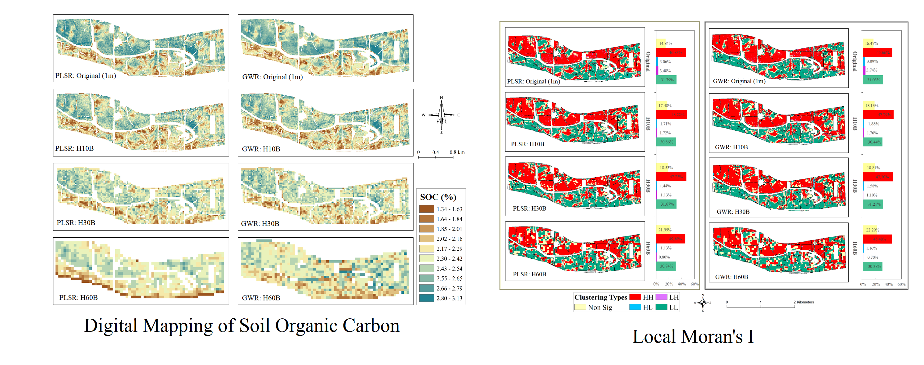
2.1. Study Area and Soil Samples

The study area (385.45 ha) is located in a watershed in the southeast of Iowa, USA (41°44′09″N, 91°56′51″E) (Figure 1). The major crop types are corn and soybeans in this area. The geography of Iowa is generally rolling hills. The elevation of the sturdy region ranges from 756.57 to 881.00 m. The climate of Iowa is a humid continental climate, and the mean annual precipitation is 903.70 mm, with the mean snowfall being 104.18 mm. The mean annual temperature is 9.80 °C, ranging from −11.60 °C to 18.30 °C. The major soil types of the study region were silty clay loam, clay loam, and silt loam [44]. Fifty surface soil samples (0–15 cm) were collected on October 2015, and another 145 surface soil samples (0–15 cm) were collected on March 2016, both by a grid soil sampling strategy of 130 m. The first soil sampling plan was used to understand the soil background knowledge in the study region, and the second soil sampling plan was to collect more soil samples and further excavate the potential of hyperspectral imaging in digital soil mapping. Nicked soil samples were collected from bare soils of a farmland, and one representative soil sample was mixed by five soil subsamples from the four corners and one center of a 1 m² square. Soil samples were ground with a porcelain mortar and passed through a 2 mm stainless steel sieve after air-drying at an indoor temperature (20–25 °C) for 14 days. The CHNS combustion gas analyzer (Vario El Cube, Elementar, Germany) [45] was used for measuring the SOC contents. Prior to the analysis, the soil inorganic carbon related materials were removed by acidification with HCl (4 mol/L). Fourteen outliers of soil samples were discarded based on the Chauvenet’s criterion [46].

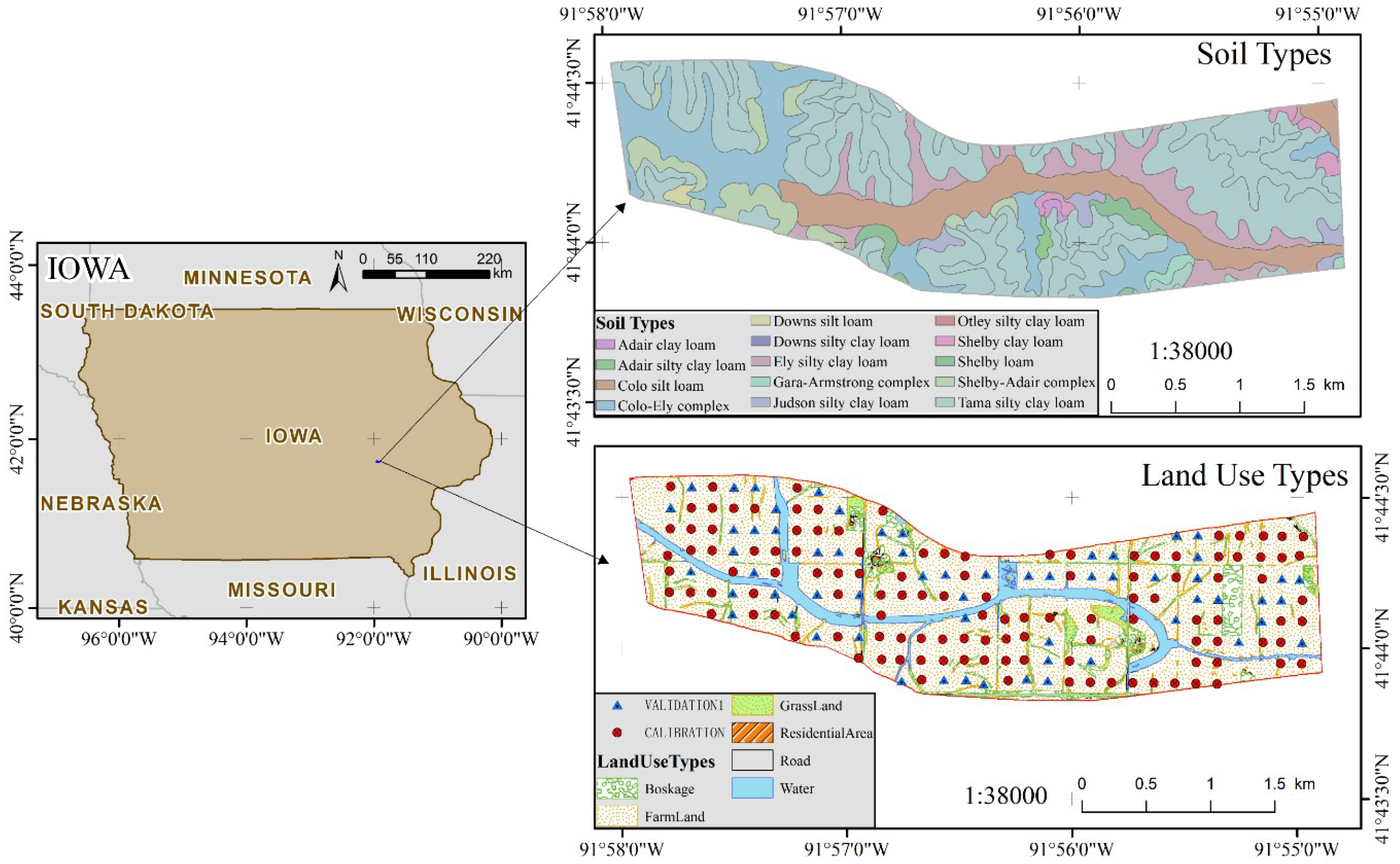
2.2. Airborne Hyperspectral Images

The Headwall Micro-Hyperspec airborne sensors (SpecTIR LLC) of Micro-Hyperspec VNIR imaging spectrometer (A-Series, 400–100 nm) and Micro-Hyperspec near infrared (NIR) imaging spectrometer (X-Series, 900–1700 nm) carried on the helicopter were used to obtain the aerial hyperspectral images on 19 November 2015. Not long ago, the land was ploughed and there were no crops or crop residues on the land surface, thus the hyperspectral images can reflect the spectral reflectance of the bare soil. The A-Series spectrometer records signals from 380 to 1000 nm in 1.9 nm contiguous bands (325 spectral bands in total), and the X-Series spectrometer captures images from 900 to 1700 nm in 12.9 nm contiguous bands (67 spectral bands in total). The instantaneous field of view (IFOV) of the A-Series and X-series was 30.8° and 20.9°, respectively. The two sensors were carried by a helicopter platform at a height of 2800 m. HRS images at a spatial resolution of 1 m were collected between 10:00 am and 2:00 pm to ensure enough bright sunlight under clear-sky conditions. Geometric corrections were performed in the Hyperspec III software with SpectralView, and an orthorectified digital aerial photograph of 1 m spatial resolution was used for geometric corrections. The calibration files were used for the radiometric and wavelength calibrations before and after sensor mobilization. The Fast Line-of-sight Atmospheric Analysis of Hypercubes (FLAASH) was used for atmospheric calibration, and transformed the spectral radiance into spectral reflectance.

The study area comprises mainly bare soils (82.41%) with the remaining area covered by urban built-up areas, water, vineyards, and vegetation. Prior to data analysis, spectral regions spanning from 380 to 430 nm, from 950 to 1000 nm, and from 1350 to 1420 nm, were removed because of the absorption by water vapor in the atmosphere. The random noise of the spectra was reduced by the Savitzky–Golay smoothing (SG) technique with a moving window of 15 nm. The background noise of spectral radiance was removed by the log (10) transform. A scatter-corrective method named standard normal variate (SNV) was employed to partially remove undesired scatter- or particle-sized information from the spectral reflectance. The pre-processing methods of SG, log(10), and SNV were used to guarantee the consistency of the calibration datasets.

The original HRS images (spatial resolution 1 m) were resampled into three spatial resolutions (10 m, 30 m, 60 m) using bilinear interpolation (BI), cubic convolution interpolation (CC), and nearest neighbor (NN) resampling methods (Figure 2). The theoretical basis of NN, BI, and CC resampling methods can be found in Lehmann et al. [49], Schultz and Stevenson [50], and Keys [51]. The resampling procedure was performed in the ENVI environment (Version 5.1, Exelis Visual Information Solutions, Inc., CO, USA).

2.3. The Prediction Models

In this paper, the soil-spectral models were constructed by PLSR and geographically weighted regression (GWR) models for predicting SOC contents. PLSR as a statistical technique can project the explanatory variables and the explained variables to a new space [52]. It has been used for predicting soil properties by the VNIR spectral reflectance in chemometric and quantitative spectral analyses [53,54]. The PLSR algorithm selects successive orthogonal factors that maximize the covariance between the explanatory variables (hyperspectral data) and the explained variable (SOC data). More details on the PLSR algorithm can be found in Harald and Paul [55]. The PLSR formulas are as follows:

$${\widehat{Z}}_{PLSR}\left(x_i,y_i\right)={\displaystyle \sum }_{k=0}^p{\widehat{\beta }}_k·q_k\left(x_i,y_i\right),\hspace{1em}i=1,\dots .,n$$

(1)

$$q_k\left(x_i,y_i\right)={\displaystyle \sum }_{j=1}^m{l}_j^{\prime }·X_j\left(x_i,y_i\right),\hspace{1em}i=1,\dots .,n$$

(2)

where ${\widehat{Z}}_{PLSR}\left(x_i,y_i\right)$ is the SOC content estimated by $\mathrm{PLSR}$ at geographical location $\left(x_i,y_i\right)$; $q_k\left(x_i,y_i\right)$ is the transferred components of the latent variables (LVs) from the hyperspectral reflectance; ${\widehat{\beta }}_k$ is the estimated drift model coefficients; p is the number of LVs; $X_j\left(x_i,y_i\right)$ is the hyperspectral reflectance of the soil sample; m is the total number of spectral wavelengths; $l_j^{\prime }$ is the eigenvector of the PLSR model. The PLS toolbox (Version 7.9.3, Eigenvector Research, Inc., Wenatchee, WA, USA) was used to operate the PLSR model in MATLAB (R2008a, MathWorks, Inc., Natick, MA, USA).

GWR as a spatial analysis technique can model the local relationships between the explanatory variables (hyperspectral data) and the explained variable (SOC data), and then construct a separate linear regression model for every location in the study region. The assumption of GWR is that the strength and direction of the relationship between the hyperspectral images and SOC may be modified by neighboring factors. The LVs extracted from PLSR were used as explanatory variables in GWR. GWR extends the traditional regression framework by allowing the relationships between the independent and dependent variables to vary by locality [56,57,58]. The GWR model is expressed in Equation (3):

$${\widehat{Z}}_{GWR}\left(x_i,y_i\right)={\displaystyle \sum }_{k=1}^p{\beta }_0\left(x_i,y_i\right)+{\displaystyle \sum }_{k=1}^p{\beta }_k\left(x_i,y_i\right)\times q_k\left(x_i,y_i\right)+\epsilon \left(x_i,y_i\right),\hspace{1em}i=1,\dots ,n$$

(3)

where ${\widehat{Z}}_{GWR}\left(x_i,y_i\right)$ is the predicted SOC content by GWR; ${\beta }_0\left(x_i,y_i\right)$ is the intercept at geographical location $\left(x_i,y_i\right)$; ${\beta }_k\left(x_i,y_i\right)$ are the coefficients; $q_k\left(x_i,y_i\right)$ is the explanatory variables of LVs; p is the number of LVs extracted from PLSR;$\epsilon \left(x_i,y_i\right)$ is the error term. The GWR model was operated by ArcGIS (Version 10.4.1, Esri Inc., Redlands, CA, USA), and the optimal bandwidth was determined by the corrected Akaike information criterion (AICc).

2.4. Evaluation Indices

The dataset is divided into two groups, one group for the calibration of the model (120, two thirds of the dataset), and a second group used for validation (61, one third of the database). The Y values are sorted in an ascending order. The method starts by selecting the sample with the lower Y value, and placing it in a validation set. Then, the next two samples are placed in the calibration set, and the procedure is continued by alternately placing the following sample in the validation set and the next two samples in the calibration set. Such a process would ensure a relatively equal distribution of the samples in both sub-datasets. The root mean square error and R² of the calibration dataset (RMSEC and R²C) were used for checking the modeling accuracy of SOC prediction models. The RMSE and R² of the validation dataset (RMSEP and R²P), and the ratio of performance to the inter–quartile range (RPIQ) were used to verify the predictive ability of the soil models [59,60].

$$R^2=1-\frac{{{\displaystyle \sum }}_{i=1}^n{\left(y_i-{\widehat{y}}_i\right)}^2}{{{\displaystyle \sum }}_{i=1}^n{\left(y_i-\overline{y}\right)}^2},$$

(4)

$$\mathrm{RMSE}=\sqrt{\frac{1}{n}{\displaystyle \sum }_{i=1}^n{\left(y_i-{\widehat{y}}_i\right)}^2},$$

(5)

$$\mathrm{RPIQ}=\frac{\mathrm{Q}3-\mathrm{Q}1}{{\mathrm{RMSE}}_p},$$

(6)

where n is the number of soil samples; $y_i$ is the measured SOC content; ${\widehat{y}}_i$ is the predicted SOC content; $\overline{y}$ is the mean value of all the measured SOC. Q3 is the third quarter of measured SOC content, and Q1 the first quarter of SOC contents in the validation dataset. Generally, a model that performs well would have large values of R² and RPIQ as well as a small RMSE value.

3. Results

3.1. Descriptive Statistics of SOC

Table 1. Statistical descriptions of the soil organic carbon contents.

	Number	Range (%)	Minimum (%)	Maximum (%)	Mean (%)	S.D. (%)	Skewness	CV	C0/(C0 + C)
Calibration	120	1.84	1.31	3.14	2.34	0.38	−0.65	16.05%	59.46%
Validation	61	1.55	1.43	2.98	2.40	0.28	−0.93	11.79%	41.84%
Whole	181	1.84	1.31	3.14	2.36	0.35	0.74	14.72%	58.62%

Note: St.D: standard deviation, CV: coefficient of variation, C₀: nugget value, C₀ + C: sill value, C₀/(C₀+C): the ratio of nugget value to sill value. The semivariogram function was estimated by the spherical model.

shows the descriptive statistics of the calibration, validation, and whole datasets. The range of SOC contents in the calibration datasets varies between 1.31% and 3.14%. This range was the same as that for the whole dataset and was lager than the validation dataset, which ranged from 1.43% to 2.98%. Thus, the separation method can provide representative soil samples for training and validation. The skewness values of these datasets were −0.65, −0.93, and 0.74, indicating an approximately normal distribution. The corresponding standard deviation values were 0.38%, 0.28%, and 0.35%, and the coefficient of variances were 16.05%, 11.79%, and 14.72% for the calibration, validation, and whole datasets, respectively. Therefore, the dispersion degree of the SOC was small in this study region, and this can further help evaluate the predictive ability of the models. The semivariogram function estimated by the spherical model was used to reveal the spatial autocorrelation of SOC contents. The ratios of nugget value (C₀) to sill value (C₀+C) of SOC contents in calibration, validation, and whole datasets were 59.46%, 41.84%, and 58.62%, respectively, which showed that moderate spatial autocorrelation (0.25 < C₀/(C₀+C) < 0.75) existed in the SOC contents of the soil samples [61].

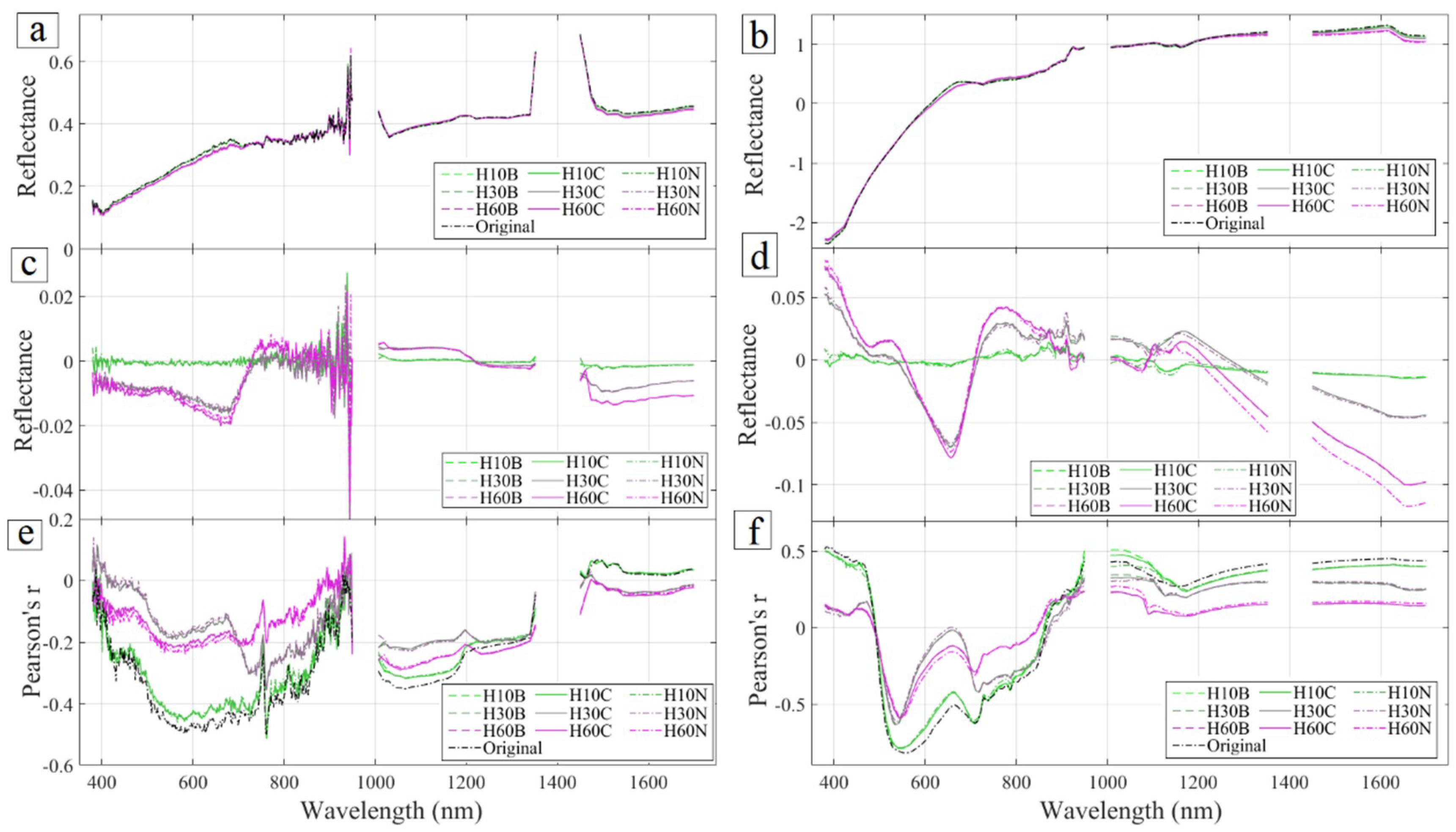
3.2. Resampled Hyperspectral Reflectance

Figure 3 shows the spectral reflectance of the original HRS image (1 m) and its resampling images, as well as the preprocessed spectral reflectance. The original and preprocessed spectral reflectance decreased with the descending of the spatial resolution (Figure 3a,b). This phenomenon may be explained by the spectral mixture at the coarse spatial resolution that resulted in smooth spectral reflectance curves. Figure 3c,d presents the deviation values of the resampled spectral reflectance to the original spectral reflectance. The difference between spectral reflectance of the HRS images at 10 m and the original spectral reflectance was much smaller than that at 30 m and 60 m. Moreover, the deviation values varied with the wavelengths, and large errors were expected with the degradation of spatial resolution. The spectral reflectance values provided by three resampling methods do not have much difference. Figure 3e,f shows the Pearson’s correlation coefficients between the spectral reflectance and SOC at different wavelengths. The spectral reflectance has a strong relationship with SOC in the visible wavelengths (400–800 nm), and this relationship weakens with the reduction of spatial resolution. Moreover, as shown in Figure 3f, the preprocessing methods can enhance this relationship. Overall, spatial resolution has a strong influence on spectral reflectance, whereas the resampling methods have minor effects.

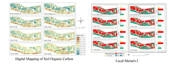
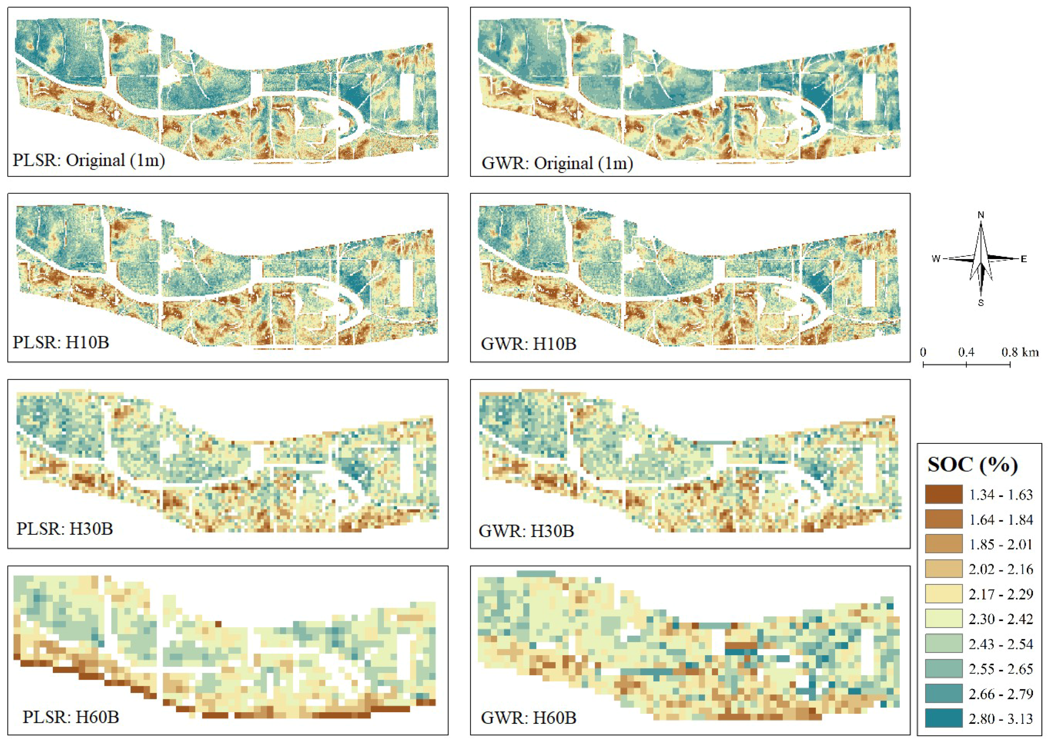
3.3. SOC Predictions

Table 2. Assessment of soil organic carbon (SOC) predictions from hyperspectral images at different spatial resolutions using PLSR and GWR models.

	PLSR						GWR
	Num.LVs	RMSEC	RMSEP	R2C	R2P	RPIQ	RMSEC	RMSEP	R2C	R2P	RPIQ
Original	4	0.165	0.159	0.797	0.708	1.957	0.138	0.155	0.857	0.814	2.003
H10B	4	0.181	0.183	0.754	0.609	1.697	0.16	0.171	0.807	0.802	1.813
H10C	4	0.184	0.194	0.747	0.559	1.603	0.163	0.181	0.801	0.793	1.713
H10N	4	0.18	0.196	0.759	0.551	1.583	0.160	0.186	0.808	0.788	1.667
H30B	5	0.226	0.222	0.617	0.45	1.400	0.220	0.216	0.639	0.646	1.435
H30C	5	0.227	0.232	0.613	0.406	1.342	0.223	0.227	0.630	0.638	1.366
H30N	5	0.235	0.250	0.587	0.33	1.242	0.228	0.246	0.611	0.607	1.260
H60B	6	0.259	0.267	0.497	0.382	1.166	0.247	0.267	0.543	0.497	1.161
H60C	6	0.260	0.270	0.494	0.381	1.151	0.250	0.267	0.533	0.502	1.161
H60N	6	0.257	0.274	0.505	0.417	1.134	0.237	0.273	0.578	0.535	1.136

Note: PLSR: partial least square regression, GWR: geographically weighted regression model, LVs: latent variables, RMSEC: the root mean square error of the calibration model, R²C: R² of the calibration model, R2P: R² of the prediction model, RMSEP: the root mean square error of the prediction model, RPIQ: the ratio of performance to inter-quartile range, RPD: the residual prediction deviation. H10B means the hyperspectral spectral image with the spatial resolution of 10 m by the bilinear interpolation, C means the cubic convolution interpolation, and N means the nearest neighbor resampling.

shows the evaluation indices of PLSR and GWR for predicting SOC contents at different spatial resolutions (1, 10, 30, and 60 m) by using different resampling methods (BI, NN, and CC). To guarantee the comparability and robustness of the prediction models, the number of the latent variables was kept constant for PLSR and GWR at the same spatial resolutions. The evaluation indices showed that the prediction accuracy of SOC decreased with the decrease in spatial resolution. PLSR and GWR yielded the highest R²C (0.797 and 0.857), R²P (0.708 and 0.691), and RPIQ (1.957 and 1.905), and the lowest RMSEC (0.165 and 0.138) and RMSEP (0.159 and 0.163) by using the original hyperspectral reflectance. Compared with the spatial resolution, the different resampling methods have a weaker influence on the prediction accuracy of SOC. The RPIQ values of PLSR were 1.697, 1.400, and 1.166, and the RPIQ values of GWR were 1.595, 1.364, and 1.165 for predictions derived from the BI resampled images at 10 m, 30 m, and 60 m, respectively. The RPIQ values of PLSR were 1.697, 1.603, and 1.583, and the RPIQ values of GWR were 1.813, 1.713, and 1.667 for the prediction of SOC from the BI resampled image at 10 m. At each spatial resolution, the performance of the predictive models built upon the BI-based resampled images was superior to that of the models built upon NN and CC-based resampled images. In addition, the performance of GWR was better than PLSR among different spatial scales. Thus, GWR could use the spatial autocorrelation to construct a better soil-spectral model.

The calibrated PLSR and GWR models were applied to the spectral reflectance of bare soils for characterizing SOC contents, and the BI resampling method was used (Figure 4). In these predicted SOC maps, spatial patterns of SOC contents were very similar across spatial resolutions. The SOC value ranged from 1.34% to 3.13%, with high values in the north of the study region and low values in the southern region. As the spatial resolution degraded, the block effects of SOC became more obvious. Although SOC maps produced by PLSR and GWR were very similar, those produced by GWR were relatively smooth.

4. Discussion

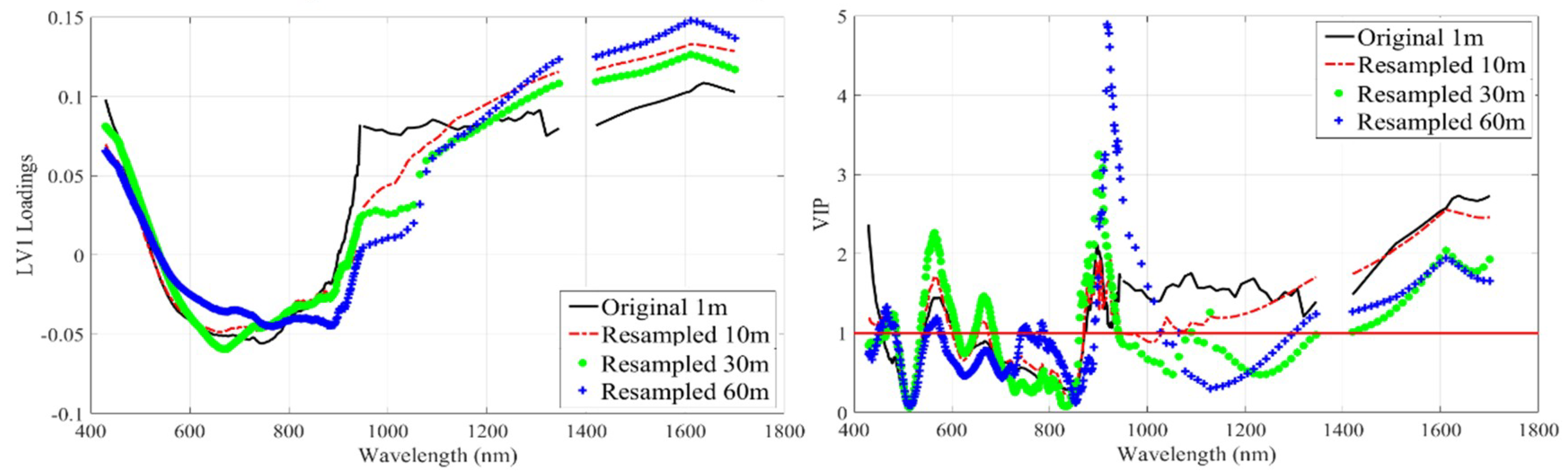
4.1. Influential Factors in Predicting SOC

The prediction accuracy of SOC contents may be influenced by both internal and external factors. The internal factors are related to satellite sensors, including spectral range, spectral resolution, spatial resolution, IFOV, and signal-to-noise ratio [62]. The external factors include atmospheric effects, geometric distortion, vegetation cover, and view geometry [63]. Among all these factors, spectral resolution and spatial resolution are of importance in digital soil mapping [38,64]. Most of the hyperspectral sensors have a spectral resolution of less than 10 nm, while the band depth of most surface materials is about 20–40 nm [65]. Thus, spectral resolution is rarely an issue for predicting soil properties from hyperspectral images [38]. A coarse spatial resolution may lead to a pixel that has a composite spectra of diversified materials in that pixel [66]. It is difficult to ensure a one-to-one correspondence between the soil samples and the hyperspectral reflectance. This study found that the SOC prediction accuracy was influenced by spatial resolution, similar to Gomez, Oltra-Carrio, Bacha, Lagacherie and Briottet [38]. To further explore the influence of spatial resolution on the hyperspectral analysis, the first latent variable (LV1) loading values on different wavelengths at four spatial resolutions were revealed (Figure 5a), and the variable importance in projection (VIP) was used to show the significant bands (Figure 5b). VIP is one most popular variable selection methods at present in the PLSR method, and it was proposed by Wold et al. [67]. VIP scores are useful in understanding the contribution rates of the spectral reflectance of soil samples (X space predictor variables) to SOC content (y variance), and the VIP value of 1 is one useful boundary to select the larger contribution spectral bands. LV1 had a positive relationship with the spectral reflectance from 400 to 500 nm and from 900 to 1700 nm, and had a negative relationship with the spectral reflectance from 500 to 900 nm. Significant variations in the LV1 loading values were found from 600 to 900 nm and from 1200 to 1800 nm at different spatial resolutions. The most important bands were located at 580 nm, 670 nm, 900 nm and from 1350 to 1700 nm (VIP value > 1). Meanwhile, the spectral bands of the hyperspectral images with the spatial resolution of 1 m and 10 m have more sensitive bands than the spatial resolution of 30 m and 60 m, especially in the NIR bands (900–1000 nm). Thus, the reduction of the spatial resolution has stronger influence on the NIR bands than the visible bands.

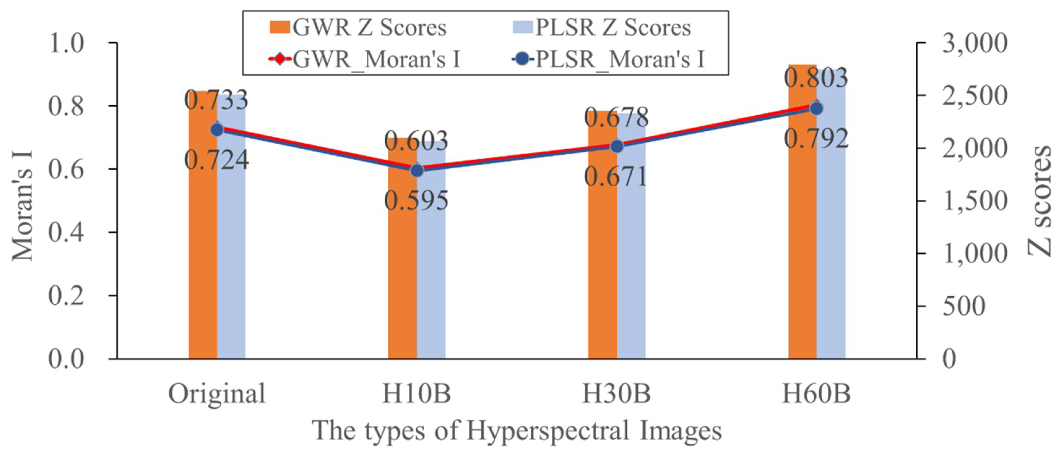
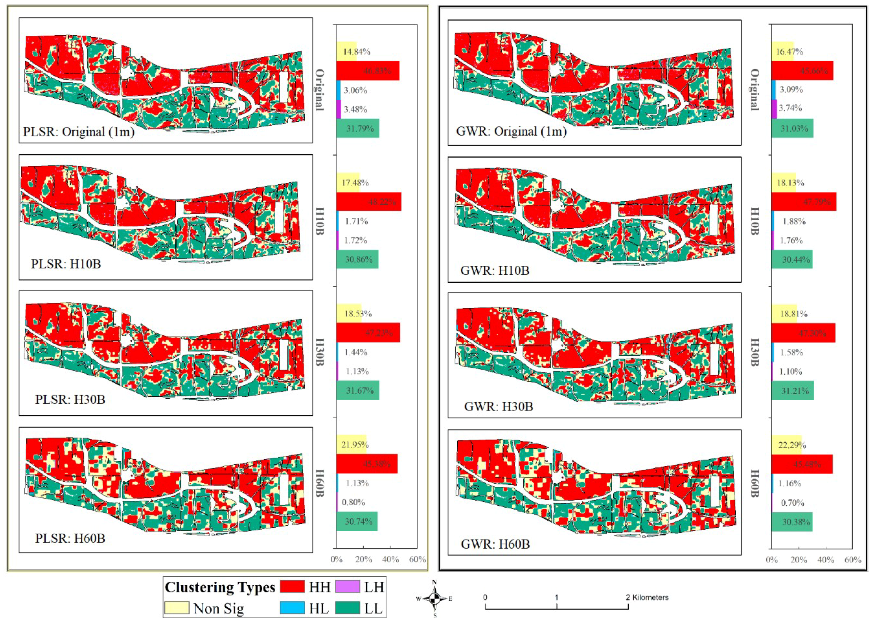
4.2. Spatial Autocorrelation of SOC at Different Spatial Scales

To reveal the spatial autocorrelation in SOC maps, the Moran’s I of the SOC maps predicted from the HRS images were calculated (Figure 6). Results showed that the SOC maps exhibited strong spatial clustering features since the Moran’s I value was larger than 0.595 and the Z score was larger than 2560. The Moran’s I values of SOC predicted from the original HRS image using PLSR and GWR were 0.733 and 0.724, and those of SOC predicted from the BI resampled HRS image at 10 m using PLSR and GWR were 0.603 and 0.595. The main reason can be due to the basic theory of the resampling methods that the new pixel value was calculated from four nearest points (1 m × 1 m, 4 pixels) to the central point to replace the original matrix (10 m × 10 m, 100 pixels), thus the resampling method will lose more information from the original matrix. Although one larger pixel unit has a larger scope, it cannot obtain more environmental objects, thus the resampled hyperspectral images reduced the spatial autocorrelation of SOC. For the resampled images from the spatial resolution of 10 m to 60 m, the spatial autocorrelation of the SOC map increased, mainly because more soil units were clustered into one unit with the degradation of spatial resolution, leading to an increase of the similarity among neighboring units. One pixel unit can represent a larger range, and this can smooth the SOC contents. Thus, the reduction of the spatial resolution can improve the spatial autocorrelation of SOC. Only a few studies have considered the spatial autocorrelation of soil properties to improve the performance of soil prediction models [33,68,69]. The evaluation indices indicated that the predictive ability of GWR was better than PLSR, and the Anselin Local Moran’s I was calculated to evaluate the local spatial autocorrelation of the SOC map (Figure 7). The non-significance values increased with the reduction of spatial resolution. The total percentages of high–low and low–high values (outliers) decreased with the degradation of spatial resolution. The high–low and low–high values mean a high value surrounded by features with low values or a low value surrounded by features with high values, thus less and less outliers were detected by the Local Moran’s I with the increase of the pixel unit, and more and more clustering characteristics could be easily found. Thus, the descending of spatial resolution can improve the spatial autocorrelation of the SOC map. The global Moran’s I and Anselin Local Moran’s I showed that there was a very small difference between the SOC maps predicted by PLSR and GWR at one same spatial resolution. However, although the evaluation indices showed that the GWR was better than PLSR, all of them can provide similar SOC maps through hyperspectral images. Nonetheless, the total percentages of high–low and low–high values for PLSR were 6.54%, 3.43%, 2.57%, and 1.93%, and for GWR were 6.83%, 3.64%, 2.68%, and 1.86% at the spatial resolutions of 1 m, 10 m, 30 m, and 60 m, respectively. Thus, the outliers of SOC can be easily obtained by GWR relative to PLSR. GWR was more sensitive to the outliers of SOC content than PLSR in digital soil mapping.

5. Conclusions

The VNIR hyperspectral imaging technology provides a promising tool for mapping topsoil properties in a timely and inexpensive way. In this study, the airborne hyperspectral images (400–1700 nm) acquired by the Headwall Micro-Hyperspec airborne sensors were used to characterize the spatial distribution of SOC contents. BI, NI, and CC were used to rescale the original hyperspectral image (1 m) into three new spatial resolutions (10 m, 30 m, and 60 m). The PLSR and GWR methods were used to construct the soil spectral models, and then the relationships between the prediction accuracy and the spatial resolution were explored. In addition, the influence factors of the soil spectral models, the uncertainty, and the spatial variability of SOC were discussed in this study.

(1) Results showed that the original and resampled VNIR hyperspectral images could be used to predict SOC through PLSR and GWR with the RPIQ values of 1.957 and 2.003. The prediction accuracy of SOC decreased with the decrease in spatial resolution, for the RPIQ values of PLSR were from 1.957 to 1.134, and of GWR were from 2.003 to 1.136. The resampling methods have weaker influence on SOC prediction accuracy, for the differences of RPIQ values of NN, BI and CC resampling methods were 0.146, 0.175 and 0.025 in the spatial resolutions of 10 m, 30 m and 60 m.

(2) The SOC prediction uncertainty mainly resulted from the soil spectral models and the spatial scale. The most important bands were located at 580 nm, 670 nm, 900 nm and from 1350 to 1700 nm (VIP value > 1), and the reduction of the spatial resolution has a stronger influence on the NIR bands than the visible bands.

(3) The Moran’s I values of SOC maps predicted by PLSR and GWR were 0.724 and 0.733 which showed that the spatial autocorrelation existed in SOC maps. The resampling of the hyperspectral images decreased the spatial autocorrelation and the degradation of the spatial resolution can enhance the spatial dependence. GWR was more sensitive to the outliers of SOC content than PLSR in digital soil mapping.

This study provides a basis to improve the design and configuration of space-borne sensors, especially in terms of spatial resolutions and signal-to-noise ratio. As the assessment of HRS maps is not a trivial task, future research refinements can be made on soil sampling strategies.

References

1. Lal, R. Global potential of soil carbon sequestration to mitigate the greenhouse effect. Crit. Rev. Plant Sci. 2003, 22, 151–184. [Google Scholar] [CrossRef]
2. Arnold, R.W. Role of soil survey in obtaining a global carbon budget. Soils Glob. Chang. 1995, 21, 257–263. [Google Scholar]
3. Kempen, B.; Brus, D.J.; Stoorvogel, J.J.; Heuvelink, G.; de Vries, F. Efficiency comparison of conventional and digital soil mapping for updating soil maps. Soil Sci. Soc. Am. J. 2012, 76, 2097–2115. [Google Scholar] [CrossRef]
4. Forkuor, G.; Hounkpatin, O.K.; Welp, G.; Thiel, M. High resolution mapping of soil properties using remote sensing variables in south-western Burkina Faso: A comparison of machine learning and multiple linear regression models. PloS ONE 2017, 12, e0170478. [Google Scholar] [CrossRef]
5. Zeraatpisheh, M.; Ayoubi, S.; Jafari, A.; Tajik, S.; Finke, P. Digital mapping of soil properties using multiple machine learning in a semi-arid region, central Iran. Geoderma 2019, 338, 445–452. [Google Scholar] [CrossRef]
6. Davidson, E.A.; Janssens, I.A. Temperature sensitivity of soil carbon decomposition and feedbacks to climate change. Nature 2006, 440, 165–173. [Google Scholar] [CrossRef] [Green Version]
7. Adamchuk, V.I.; Allred, B.; Doolittle, J.; Grote, K.; Rossel, R.; Ditzler, C.; West, L. Tools for proximal soil sensing. In Soil Survey Manua; Ditzler, C., West, L., Eds.; U.S. Department of Agriculture: Lincoln, NE, USA, 2015; Volume 6, pp. 1–31. [Google Scholar]
8. Viscarra Rossel, R.A.; Webster, R.; Bui, E.N.; Baldock, J.A. Baseline map of organic carbon in Australian soil to support national carbon accounting and monitoring under climate change. Glob. Chang. Biol. 2014, 20, 2953–2970. [Google Scholar] [CrossRef] [Green Version]
9. Dhawale, N.M.; Adamchuk, V.I.; Prasher, S.O.; Rossel, R.A.V.; Ismail, A.A.; Whalen, J.K.; Louargant, M. Comparing Visible/NIR and MIR Hyperspectrometry for Measuring Soil Physical Properties. In Proceedings of the International Conference of American Society of Biological Engineers, Montreal, QC, Canada, 13–16 July 2014; American Society of Agricultural and Biological Engineers: Saint Joseph, MI, USA, 2014. [Google Scholar] [CrossRef]
10. Terra, F.S.; Rossel, R.A.V.; Demattê, J.A. Spectral fusion by Outer Product Analysis (OPA) to improve predictions of soil organic C. Geoderma 2019, 335, 35–46. [Google Scholar] [CrossRef]
11. Hobley, E.U.; Prater, I. Estimating soil texture from vis–NIR spectra. Eur. J.Soil Sci. 2019, 70, 83–95. [Google Scholar] [CrossRef]
12. Kawamura, K.; Tsujimoto, Y.; Nishigaki, T.; Andriamananjara, A.; Rabenarivo, M.; Asai, H.; Rakotoson, T.; Razafimbelo, T. Laboratory Visible and Near-Infrared Spectroscopy with Genetic Algorithm-Based Partial Least Squares Regression for Assessing the Soil Phosphorus Content of Upland and Lowland Rice Fields in Madagascar. Remote Sens. 2019, 11, 506. [Google Scholar] [CrossRef]
13. Shi, T.Z.; Chen, Y.Y.; Liu, H.Z.; Wang, J.J.; Wu, G.F. Soil Organic Carbon Content Estimation with Laboratory-Based Visible-Near-Infrared Reflectance Spectroscopy: Feature Selection. Appl. Spectrosc. 2014, 68, 831–837. [Google Scholar] [CrossRef] [PubMed]
14. Viscarra Rossel, R.A.; Webster, R. Predicting soil properties from the Australian soil visible-near infrared spectroscopic database. Eur. J. Soil Sci. 2012, 63, 848–860. [Google Scholar] [CrossRef]
15. Fang, Q.; Hong, H.; Zhao, L.; Kukolich, S.; Yin, K.; Wang, C. Visible and near-infrared reflectance spectroscopy for investigating soil mineralogy: a review. J. Spectrosc. 2018, 2018, 14. [Google Scholar] [CrossRef]
16. Cambou, A.; Cardinael, R.; Kouakoua, E.; Villeneuve, M.; Durand, C.; Barthes, B.G. Prediction of soil organic carbon stock using visible and near infrared reflectance spectroscopy (VNIRS) in the field. Geoderma 2016, 261, 151–159. [Google Scholar] [CrossRef]
17. Ji, W.J.; Shi, Z.; Huang, J.Y.; Li, S. In Situ Measurement of Some Soil Properties in Paddy Soil Using Visible and Near-Infrared Spectroscopy. PLoS ONE 2014, 9, 11. [Google Scholar] [CrossRef]
18. Gopal, B.; Shetty, A.; Ramya, B.J. Prediction of the presence of topsoil nitrogen from spaceborne hyperspectral data. Geocarto Int. 2015, 30, 82–92. [Google Scholar] [CrossRef]
19. Goetz, A.F.H. Three decades of hyperspectral remote sensing of the Earth: A personal view. Remote Sens. Environ. 2009, 113, S5–S16. [Google Scholar] [CrossRef]
20. Gomez, C.; Rossel, R.A.V.; McBratney, A.B. Soil organic carbon prediction by hyperspectral remote sensing and field vis-NIR spectroscopy: An Australian case study. Geoderma 2008, 146, 403–411. [Google Scholar] [CrossRef]
21. Stevens, A.; Miralles, I.; Wesemael, B.V. Soil Organic Carbon Predictions by Airborne Imaging Spectroscopy: Comparing Cross-Validation and Validation. Soil Sci. Soc. Am. J. 2012, 76, 2174–2183. [Google Scholar] [CrossRef]
22. Peon, J.; Fernandez, S.; Recondo, C.; Calleja, J.F. Evaluation of the spectral characteristics of five hyperspectral and multispectral sensors for soil organic carbon estimation in burned areas. Int. J. Wildland Fire 2017, 26, 230–239. [Google Scholar] [CrossRef]
23. Hestir, E.L.; Khanna, S.; Andrew, M.E.; Santos, M.J.; Viers, J.H.; Greenberg, J.A.; Rajapakse, S.S.; Ustin, S.L. Identification of invasive vegetation using hyperspectral remote sensing in the California Delta ecosystem. Remote Sens. Environ. 2008, 112, 4034–4047. [Google Scholar] [CrossRef]
24. Viscarra Rossel, R.A.; McGlynn, R.N.; McBratney, A.B. Determining the composition of mineral-organic mixes using UV-vis-NIR diffuse reflectance spectroscopy. Geoderma 2006, 137, 70–82. [Google Scholar] [CrossRef]
25. Viscarra Rossel, R.; Behrens, T.J.G. Using data mining to model and interpret soil diffuse reflectance spectra. Geoderma 2010, 158, 46–54. [Google Scholar] [CrossRef]
26. Liu, Y.; Pan, X.; Wang, C.; Li, Y.; Shi, R. Predicting Soil Salinity with Vis–NIR Spectra after Removing the Effects of Soil Moisture Using External Parameter Orthogonalization. PLoS ONE 2015, 10, e0140688. [Google Scholar] [CrossRef] [PubMed]
27. Lagacherie, P.; Sneep, A.-R.; Gomez, C.; Bacha, S.; Coulouma, G.; Hamrouni, M.H.; Mekki, I. Combining Vis–NIR hyperspectral imagery and legacy measured soil profiles to map subsurface soil properties in a Mediterranean area (Cap-Bon, Tunisia). Geoderma 2013, 209, 168–176. [Google Scholar] [CrossRef]
28. Gupta, A.; Vasava, H.B.; Das, B.S.; Choubey, A.K. Local modeling approaches for estimating soil properties in selected Indian soils using diffuse reflectance data over visible to near-infrared region. Geoderma 2018, 325, 59–71. [Google Scholar] [CrossRef]
29. Farrukh, N. Evaluation of the eo-1heperion Image for Assessment of Soil Organic Carbon in Faizabad Watershed. Master’s Thesis, University of Central Asia, Kyrgyz Republic, 2011. [Google Scholar]
30. Dotto, A.C.; Diniz Dalmolin, R.S.; ten Caten, A.; Grunwald, S. A systematic study on the application of scatter-corrective and spectral-derivative preprocessing for multivariate prediction of soil organic carbon by Vis-NIR spectra. Geoderma 2018, 314, 262–274. [Google Scholar] [CrossRef]
31. Vasat, R.; Kodesova, R.; Boruvka, L. Ensemble predictive model for more accurate soil organic carbon spectroscopic estimation. Comput. Geosci. 2017, 104, 75–83. [Google Scholar] [CrossRef]
32. Tekin, Y.; Tumsavas, Z.; Mouazen, A.M. Comparing the artificial neural network with parcial least squares for prediction of soil organic carbon and PH at different moisture content levels using visible and near-infrared spectroscopy. Revista Brasileira de Ciência do Solo 2014, 38, 1794–1804. [Google Scholar] [CrossRef]
33. Kumar, S.; Lal, R.; Liu, D. A geographically weighted regression kriging approach for mapping soil organic carbon stock. Geoderma 2012, 189, 627–634. [Google Scholar] [CrossRef]
34. Guo, L.; Zhao, C.; Zhang, H.; Chen, Y.; Linderman, M.; Zhang, Q.; Liu, Y. Comparisons of spatial and non-spatial models for predicting soil carbon content based on visible and near-infrared spectral technology. Geoderma 2017, 285, 280–292. [Google Scholar] [CrossRef]
35. Lee, C.M.; Cable, M.L.; Hook, S.J.; Green, R.O.; Ustin, S.L.; Mandl, D.J.; Middleton, E.M. An introduction to the NASA Hyperspectral InfraRed Imager (HyspIRI) mission and preparatory activities. Remote Sens. Environ. 2015, 167, 6–19. [Google Scholar] [CrossRef]
36. Ben-Dor, E.; Kafri, A.; Varacalli, G. SHALOM: An Italian–Israeli hyperspectral orbital mission—Update. In Proceedings of the International Geoscience and Remote Sensing Symposium, Quebec City, QC, Canada, 13–18 July 2014. [Google Scholar]
37. Deng, S.; Tian, L.; Jian, L.I.; Chen, X.; Sun, Z.; Zhang, L.; Wei, A. A novel chlorophyll-a inversion model in turbid water for GF-5 satellite hyperspectral sensor—A case in Poyang Lake. J. Cent. China Normal Univ. 2018, 03, 409–415. [Google Scholar]
38. Gomez, C.; Oltra-Carrio, R.; Bacha, S.; Lagacherie, P.; Briottet, X. Evaluating the sensitivity of clay content prediction to atmospheric effects and degradation of image spatial resolution using Hyperspectral VNIR/SWIR imagery. Remote Sens. Environ. 2015, 164, 1–15. [Google Scholar] [CrossRef]
39. Shi, C.; Wang, L. Incorporating spatial information in spectral unmixing: A review. Remote Sens. Environ. 2014, 149, 70–87. [Google Scholar] [CrossRef]
40. Griffith, D.A.; Chun, Y. Spatial Autocorrelation and Uncertainty Associated with Remotely-Sensed Data. Remote Sens. 2016, 8, 535. [Google Scholar] [CrossRef]
41. Chen, S.; Feng, L.; Li, S.; Ji, W.; Shi, Z. Vis-NIR spectral inversion for prediction of soil total nitrogencontent in laboratory based on locally weighted regression. Acta Pedol. Sin. 2015, 52, 312–320. [Google Scholar]
42. Heil, J.; Häring, V.; Marschner, B.; Stumpe, B. Advantages of fuzzy k-means over k-means clustering in the classification of diffuse reflectance soil spectra: A case study with West African soils. Geoderma 2019, 337, 11–21. [Google Scholar] [CrossRef]
43. Chen, T.; CHANG, Q.-R.; Liu, J. Study of spatial interpolation of soil cd contents in sewage irrigated area based on soil spectral information assistance. Spectrosc. Spectr. Anal. 2013, 33, 2157–2162. [Google Scholar]
44. Burt, R.; Staff, S. Kellogg soil survey laboratory methods manual. In Natural Resources Conservation Services; National Soil Survey Center: Lincoln, NE, USA, 2014. [Google Scholar]
45. ISO10694, ISO. Soil Quality—Determination of Organic and Total Carbon After Dry Combustion (Elementary Analysis); ISO: Geneva, Switzerland, 1995. [Google Scholar]
46. Ross, S.M. Peirce’s criterion for the elimination of suspect experimental data. J. Eng. Technol. 2003, 20, 38–41. [Google Scholar]
47. Guo, L.; Zhang, H.; Shi, T.; Chen, Y.; Jiang, Q.; Linderman, M. Prediction of soil organic carbon stock by laboratory spectral data and airborne hyperspectral images. Geoderma 2019, 337, 32–41. [Google Scholar] [CrossRef]
48. Guo, L.; Linderman, M.; Shi, T.Z.; Chen, Y.Y.; Duan, L.J.; Zhang, H.T. Exploring the Sensitivity of Sampling Density in Digital Mapping of Soil Organic Carbon and Its Application in Soil Sampling. Remote Sens. 2018, 10, 888. [Google Scholar] [CrossRef]
49. Lehmann, T.M.; Gonner, C.; Spitzer, K. Survey: Interpolation methods in medical image processing. IEEE Trans. Med. Imaging 1999, 18, 1049–1075. [Google Scholar] [CrossRef]
50. Schultz, R.R.; Stevenson, R.L. Extraction of high-resolution frames from video sequences. IEEE Trans. Image Process. 1996, 5, 996–1011. [Google Scholar] [CrossRef]
51. Keys, R.G. Cubic convolution interpolation for digital image-processing. IEEE Trans. Acoust. Speech Signal Process. 1981, 29, 1153–1160. [Google Scholar] [CrossRef]
52. Geladi, P.; Kowalski, B.R. Partial least-squares regression: a tutorial. Anal. Chim. Acta 1986, 185, 1–17. [Google Scholar] [CrossRef]
53. Askari, M.S.; O’Rourke, S.M.; Holden, N.M. Evaluation of soil quality for agricultural production using visible-near-infrared spectroscopy. Geoderma 2015, 243, 80–91. [Google Scholar] [CrossRef]
54. Xu, L.; He, N.P.; Yu, G.R. Methods of evaluating soil bulk density: Impact on estimating large scale soil organic carbon storage. Catena 2016, 144, 94–101. [Google Scholar] [CrossRef] [Green Version]
55. Harald, M.; Paul, G. Multivariate calibration. Technometrics 1991, 1158, 61. [Google Scholar]
56. Brunsdon, C.; Fotheringham, S.; Charlton, M. Geographically weighted regression. J. R. Stat. Soc. Ser. D (The Statistician) 1998, 47, 431–443. [Google Scholar] [CrossRef]
57. Charlton, M.; Fotheringham, S.; Brunsdon, C. Geographically weighted regression. In White Paper. National Centre for Geocomputation; National University of Ireland Maynooth: Maynooth, Ireland, 2009. [Google Scholar]
58. Fotheringham, A.S.; Brunsdon, C.; Charlton, M. Geographically Weighted Regression; Wiley: New York, NY, USA, 2002. [Google Scholar]
59. Gogé, F.; Gomez, C.; Jolivet, C.; Joffre, R. Which strategy is best to predict soil properties of a local site from a national Vis–NIR database? Geoderma 2014, 213, 1–9. [Google Scholar] [CrossRef]
60. Bellon-Maurel, V.; Fernandez-Ahumada, E.; Palagos, B.; Roger, J.-M.; McBratney, A. Critical review of chemometric indicators commonly used for assessing the quality of the prediction of soil attributes by NIR spectroscopy. TrAC Trends Anal. Chem. 2010, 29, 1073–1081. [Google Scholar] [CrossRef]
61. Li, D.; Chen, Y. Computer and Computing Technologies in Agriculture: 5th IFIP TC 5, SIG 5.1 International Conference, CCTA 2011, Beijing, China, 29–31 October 2011, Proceedings; Springer Science & Business Media: Berlin, Germany, 2012. [Google Scholar]
62. Landgrebe, D.A. Signal Theory Methods in Multispectral Remote Sensing; John Wiley & Sons: Hoboken, NJ, USA, 2005; Volume 29. [Google Scholar]
63. Schowengerdt, R.A. Remote Sensing: Models and Methods for Image Processing; Academic Press: Cambridge, MA, USA, 2006. [Google Scholar]
64. Castaldi, F.; Palombo, A.; Santini, F.; Pascucci, S.; Pignatti, S.; Casa, R. Evaluation of the potential of the current and forthcoming multispectral and hyperspectral imagers to estimate soil texture and organic carbon. Remote Sens. Environ. 2016, 179, 54–65. [Google Scholar] [CrossRef]
65. Hunt, G.R. Near-infrared (1.3–2.4) μm spectra of alteration minerals—Potential for use in remote sensing. Geophysics 1979, 44, 1974–1986. [Google Scholar] [CrossRef]
66. Plaza, A. Near real-time endmember extraction from remotely sensed hyperspectral data using NVidia GPUs. In Real-Time Image and Video Processing 2010; International Society for Optics and Photonics: San Diego, CA, USA, 2010; Volume 7724, p. 772409. [Google Scholar]
67. Wold, S.; Johansson, E.; Cocchi, M. Partial Least Squares Projections to Latent Structures; Wiley & Sons: Hoboken, NJ, USA, 2002. [Google Scholar]
68. Liu, Y.; Guo, L.; Jiang, Q.; Zhang, H.; Chen, Y. Comparing geospatial techniques to predict SOC stocks. Soil Tillage Res. 2015, 148, 46–58. [Google Scholar] [CrossRef]
69. Yoon, T.K.; Noh, N.J.; Han, S.; Kwak, H.; Lee, W.K.; Son, Y. Small-scale spatial variability of soil properties in a Korean swamp. Landsc. Ecol. Eng. 2015, 11, 303–312. [Google Scholar] [CrossRef]
Figure 1. Geographical location and soil and land-use types of the study area. The soil type map was downloaded from the Online Web Soil Survey (official United States Department of Agriculture soil information), and the land-use type map was manually interpreted from the hyperspectral image by a local expert. The maps of soil types and land-use types have been used in the following references: [47,48].
Remotesensing 11 01032 g001
Figure 2. Original hyperspectral remote sensing image (1 m) and the resampled remote sensing images at different spatial resolutions (10 m, 30 m, and 60 m) by bilinear interpolation (BI), cubic convolution interpolation (CC), and nearest neighbor (NN) resampling methods. The original hyperspectral images were the same as the following references: [47,48].
Remotesensing 11 01032 g002
Figure 3. Average original (a) and preprocessed (b) spectral reflectance of the soil samples (n = 181) at different spatial resolutions (10, 30, and 60 m) resampled using the bilinear interpolation, cubic convolution interpolation, and nearest neighbor; The average deviation values between resampled spectral reflectance and the original spectral reflectance (c,d); The Pearson’s correlation coefficient between the spectral reflectance and soil organic carbon (e,f). In the symbol of H10B, H means hyperspectral images, 10 means the spatial resolution and B means the bilinear interpolation. C means the cubic convolution interpolation, and N means the near neighbor.
Remotesensing 11 01032 g003
Figure 4. Spatial patterns of soil organic carbon (SOC) contents predicted from the original and bilinear interpolation (BI)-resampled hyperspectral remote sensing (HRS) images by using partial least squares regression (PLSR) and geographically weighted regression models (GWR).
Remotesensing 11 01032 g004
Figure 5. First latent variable (LV1) loading (left) and variable importance in projection (VIP) (right) values for partial least squares regression (PLSR) models built from hyperspectral images at different spatial resolutions (1, 10, 30, and 60 m) which were resamples by the bilinear interpolation method. The horizontal lines indicate the threshold of VIP (threshold at 1), and the bilinear interpolation was used.
Remotesensing 11 01032 g005
Figure 6. Global Moran’s I of the soil organic carbon (SOC) predicted from hyperspectral images at 1, 10, 30, and 60 m which were resamples by the bilinear interpolation method. H10B means the hyperspectral spectral image with the spatial resolution of 10 m by the bilinear interpolation method, and H30B and H60B were the spatial resolutions of 30 m and 60 m, respectively.
Remotesensing 11 01032 g006
Figure 7. Anselin Local Moran’s I of the soil organic carbon (SOC) predicted from hyperspectral images at 1, 10, 30, and 60 m which were resamples by the bilinear interpolation method. H10B means the hyperspectral spectral image with the spatial resolution of 10 m by the bilinear interpolation method, and H30B and H60B were the spatial resolutions of 30 m and 60 m, respectively. HH means a statistically significant cluster of high values, LL means a statistically significant cluster of low values, HL means a high value surrounded by features with low values, and LH means a low value surrounded by features with high values.
Remotesensing 11 01032 g007