Classification of PolSAR Image Using Neural Nonlocal Stacked Sparse Autoencoders with Virtual Adversarial Regularization

1
School of Electronic, Electrical and Communication Engineering, University of Chinese Academy of Sciences, Huairou District, Beijing 101408, China
2
Institute of Electronics, Chinese Academy of Sciences, Beijing 100190, China
*
Author to whom correspondence should be addressed.
Remote Sens. 2019, 11(9), 1038; https://0-doi-org.brum.beds.ac.uk/10.3390/rs11091038
Submission received: 26 March 2019
/
Revised: 24 April 2019
/
Accepted: 28 April 2019
/
Published: 1 May 2019
(This article belongs to the Special Issue Region Based Classification (RBC), Object Based Image Analysis (OBIA) and Deep Learning (DL) for Remote Sensing Applications)
Abstract
:Polarimetric synthetic aperture radar (PolSAR) has become increasingly popular in the past two decades, for it can derive multichannel features of ground objects, which contains more discriminative information compared with traditional SAR. In this paper, a neural nonlocal stacked sparse autoencoders with virtual adversarial regularization (NNSSAE-VAT) is proposed for PolSAR image classification. The NNSSAE first extracts the nonlocal features by calculating pairwise similarity of each pixel and its surrounding pixels using a neural network, which contains a multiscale feature extractor and a linear embedding layer. The feature extraction process can relieve the negative influence of speckle noise and extract discriminative nonlocal spatial information without carefully designed parameters. Then, the SSAE maps the center pixel and the extracted nonlocal features into deep latent space in which a Softmax classifier is utilized to conduct classification. The virtual adversarial training is introduced to regularize the network, which tries to keep the network from being overfitting. The experimental results from three real PolSAR image show that the proposed NNSSAE-VAT method has proved its robustness and effectiveness and it can achieve competitive performance compared with related methods.
1. Introduction
Synthetic Aperture Radar (SAR), as a kind of active imaging sensor, has the ability of monitoring a wide area without the limitation of lighting condition and weather. One of the SAR-based techniques, namely Polarimetric SAR (PolSAR), not only inherits the advantages of SAR, but also possesses multi-polarization characteristic, by which the sensor can extract more spatial information. Due to these advantages, the analysis of PolSAR images have received extensive attention in past decades. Combined with machine learning techniques, PolSAR has been proved to be an efficient tool in many research fields, such as terrain classification, agriculture monitoring [1,2], disaster monitoring [3,4], target recognition and detection [5], and sea ice monitoring [6], etc. In this paper, we focus on PolSAR image classification. Many effective machine-learning approaches have been proposed in this field, like Wishart classifier [7,8], support vector machine (SVM) [9,10], sparse representation based classification method (SRC) [11,12], random forest [13], and so on.
To obtain terrain identification information extracted by target decomposition techniques, Lee et al. [7,8] proposed complex Wishart classifier for unsupervised PolSAR image classification using Cloude-Pottier decomposition [14], and Freeman decomposition [15], respectively. To reduce the isolated misclassified pixels, Wu et al. [16] proposed the Wishart Markov random field (WMRF) model and obtained smoother classification label map. Instead of hand-crafted features, Xie et al. [17] proposed the Wishart autoencoders to learn the latent features in PolSAR data using Wishart distance based loss function. SVM is a frequently used supervised machine-learning model in PolSAR image classification [18], for it has solid theoretical foundations and good generalization performance. In order to extract more efficient features, Zhang et al. [9] introduced the multiple-component scattering model [19] to SVM and achieved better classification performance compared with traditional Wishart classifier. Lardeux et al. [10] proposed using SVM with multifrequency PolSAR data and a set of polarimetric features to obtain higher classification accuracy. To fully utilize the sparse characteristics of polarimetric features, Zhang et al. [11] introduced the SRC [20] to PolSAR image classification. To take spatial information into consideration, Feng et al. [12] performed polarimetric contextual classification by combining SRC and superpixels. The results show that the method can relieve the negative influence of speckle noise and obtain smoother classification map. Du et al. [13] proposed random forest and its variant called rotation forest for PolSAR image classification. Even with limited training samples, the random forest based classification model can achieve promising performance.
In recent years, with the fast development of deep learning, the deep neural networks have manifested its significant superiority over the traditional machine learning approaches. Stacked autoencoders (SAE) [21,22] utilized layer-wise pre-training to learn, unsupervised, latent features contained in the data, which relieve the gradient vanishing problem and achieve better performance in PolSAR image classification task [23]. In order to enhance the rubostness of the model, Chen et al. [24] presented a self-paced learning regularized multilayer autoencoders (SPLMAE). Spatial information is also widely used in deep learning models designed for PolSAR image classification. Hou et al. [25] proposed a method combining superpixels and stacked sparse autoencoders (SSAE), which used superpixels segmentation as a refinement to the classification map. As an alternative, Zhang et al. [26] introduced local sptial information into SSAE (SSAE-LS), aiming to make SSAE automatically capture deep spatial information and reduce the negative impact of speckle noise. In recent years, convolutional neural networks (CNN) [27] have achieved excellent results in many research field. It is designed to learn the hierarchy of spatial features automatically. Zhou et al. [28] applied CNN to PolSAR image classification. The visualization results of optimized convolutional kernel shows that CNN has the capability of extracting discriminative spatial features. To preserve the correlation in the non-diagonal elements of the coherency matrix, Zhang et al. [29] proposed Complex-valued CNN, extending parameters of the deep model to complex domain and achieving better results. Despite CNN has shown promising performance on spatial information extraction and feature representation, it fails to emphasize the distinctive characteristics of the central pixel. This disadvantage can lead to ambiguous classification boarder between two different land types.
Recently, several deep learning models, which are capable to extract both discriminative spatial information and pixel features, have been proposed. Geng et al. [30] proposed a superpixel-restraint deep neural network (SRDNN). The model concatenates the superpixel-averaged features and the original features, and conduct pixel-wise classification. Inspried by a denosing method called nonlocal means filter (NLM) [31], Hu et al. [32] presented an adaptive nonlocal stacked sparse autoencoders (ANSSAE), which proposed an adaptive nonlocal feature extractor (ANFE) to obtain nonlocal features by calculating spatial similarities. Both of these two methods are pixel-wise based classification models. At training stage, they not only learn the characteristics of the original pixel, but also take mean-based nonlocal spatial information into account, which make them perform better on PolSAR image classification task compared with local spatial information methods. One defect that may limit the application of these two models is that they both need parameters to be tuned with expert knowledge, for instance, the number of superpixel for SRDNN and the value of mask coefficient for ANSSAE.
By introducing the main idea of the nonlocal means filter into deep learning, Wang et al. [33] presented the nonlocal neural networks (NLN) to capsule space-time relationship for video classification. The proposed nonlocal blocks apply nonlocal operation to the feature maps to measure the long-range correlation on spatial and temporal domains. Inspired by the nonlocal operation, we propose a PolSAR image classification method based on neural nonlocal stacked sparse autoencoders (NNSSAE). NNSSAE is composed of a neural nonlocal feature extractor (NNFE) and a SSAE. NNFE is similar in spirit with adaptive nonlocal feature extractor proposed by ANSSAE. However, all the parameters related with feature extraction are automatically optimized in the training procedure, which means no need for expert parameter tuning in feature extraction stage. SSAE is adopted to unfold the detail-reserved nonlocal spatial features extracted by NNFE and the original features, and map them into high dimension latent space. Softmax classifier [34] is introduced to conduct classification to the whole image.
Deep models have strong representing and fitting capabilities. These advantages can become a double-edged sword, for they often cause degradation on performance and overfitting while they are applied to small datasets like PolSAR images. To relieve this issue, Miyato et al. [35,36] proposed virtual adversarial training (VAT), which improves the robustness of the model by introducing prediction distribution smoothing penalty term into loss function. We introduce the VAT regularization term into training procedure, and make the model achieve better accuracy.
The main contribution of this paper is demonstrated as follows:
- We propose the neural nonlocal feature extractor, which introduces neural nonlocal similarity calculation into PolSAR image classification task to extract nonlocal spatial information around each pixel. The nonlocal spatial features generated by NNFE are automatically optimized, which improves the robustness and the classification accuracy of the model.
- In NNFE, we introduce a multiscale spatial information extractor implemented as convolution layers, which maps every pixel in image patches into latent space and considers both of their characteristics and their spatial information.
- Virtual adversarial training regularization term is introduced into the loss function to further improve the classification accuracy and the ability of generalization of the model.
The NNSSAE is validated on three real dataset and the results show that our model can achieve higher performance compared with other related models.
2. Related Works
2.1. Nonlocal Feature Extraction Methods
Nonlocal methods utilize the spatial information of pixels around one center pixel to construct its characteristics. They have many variants and have wide application. Three nonlocal methods will be introduced in this subsection. Considering that many symbols are easy to be confused with each other, we add the lower case of the corresponding abbreviation at the final of the symbol’s subscript to point out which method the symbol belongs to.
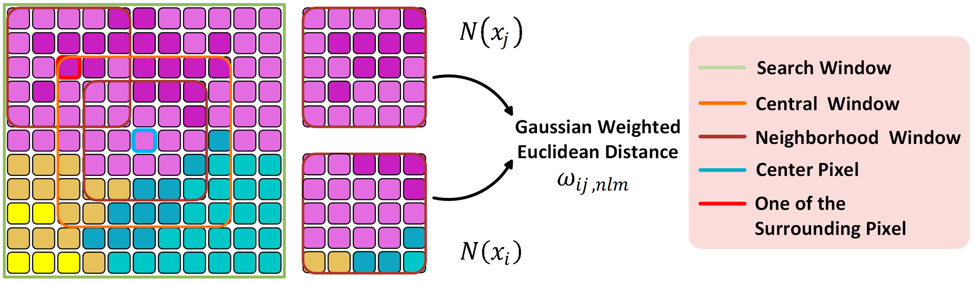
NLM is a widely used noise-reduction method that calculates the weighted sum by measuring the central pixel and its surrounding pixels’ spatial similarity. To unify the symbols used in the paper, all terms follow the ANSSAE [32] with minimum modifications. All pixels in the PolSAR image are centered with three windows: the search window, the central window and the neighborhood window, which are shown in Figure 1. The circumstance that the search window is centering at the boarder of three different kinds ground objects is considered in Figure 1 and Figure 2. Different colors of pixels represent different categories of ground objects.
Every pixel in search window is influential to the value of noise-reduction estimation of the center pixel . The central window of is denoted as , in which all of the pixels have their corresponding neighborhood windows . The weighted sum of pixels in equals the nonlocal means filtered center pixel
where the weights are simultaneously normalized and have values between 0 and 1, i.e.,
The pixels in neighborhood window are the fundamental elements participating weights calculation of the central window . The weights calculation for pixel and pixel is equivalent with calculating the normalized similarity metrics of pixels in and . The distance between and is defined by Gaussian weighted Euclidean distance, which is shown in Equation (3).
where and . denotes the variance of the Gaussian kernel. Smaller indicates that and are closer under the Gaussian weighted Euclidean distance criterion, and leads to a larger value of . The calculation of is shown in Equation (4).
where is the normalization scaling factor, and denotes the filtering parameter.
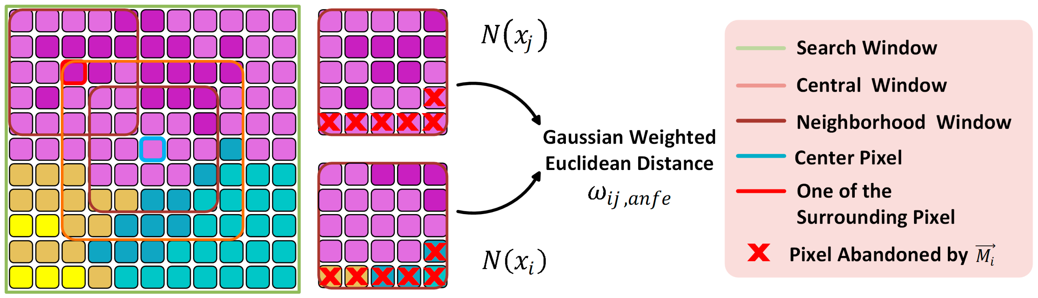
ANFE is the feature extractor of the ANSSAE proposed by Reference [32]. It introduces a hard-decision vector into the original NLM method. To avoid ambiguities in the illustration of ANFE, let be pixel in , where and . Let be the -th binary elements in the vector. At the boarder of different land types, pixels in but having different label with are denoted as . Taking into the weight calculation of NLM can lead to unexpected weight decrease if pixels are far away from the boarder, but have the same label with . To relieve this undesirable effect, is adopted to exclude singular pixels in from taking part in similarity calculation, which is depicted in Figure 2.
The calculation of is shown as follows:
where is a parameter related to the degree of the singular pixel decision, which needs expert knowledge to be tuned. The modified similarity calculation is:
where , is the number of pixels in the neighborhood window.
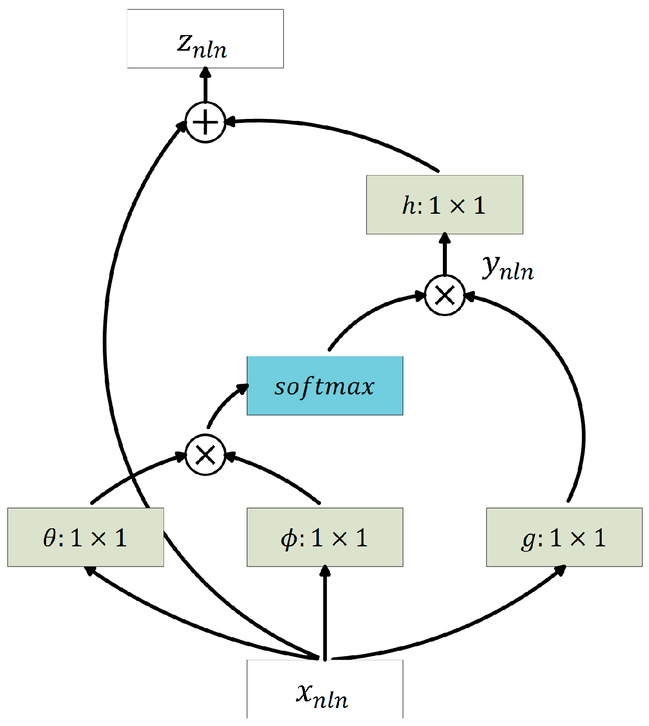
NLN is a kind of neural networks that introduce the main idea of NLM into deep learning, enabling the networks to capsule the long range correlations in feature maps [33]. As is depicted in Figure 3, weighted sum of the original features applied in nonlocal neural blocks generally follows the form of NLM, as is shown in Equation (1), while the weight calculation takes learned features into consideration, i.e.,:
where and are features of the previous layer, and are linear embeddings. Nonlocal operation is implemented in the form of exponential dot product, which is named as “the embedded Gaussian form”. denotes the normalization term. Thus, the equation introduces a softmax operation to . Then, the weighted sum equals the calculated weights multiply the corresponding linear embeddings , i.e.,
The output of the nonlocal operation equals the original feature plus the linear embeddings of . Figure 3 shows the structure of the Nonlocal block.
2.2. Virtual Adversarial Training Regularization
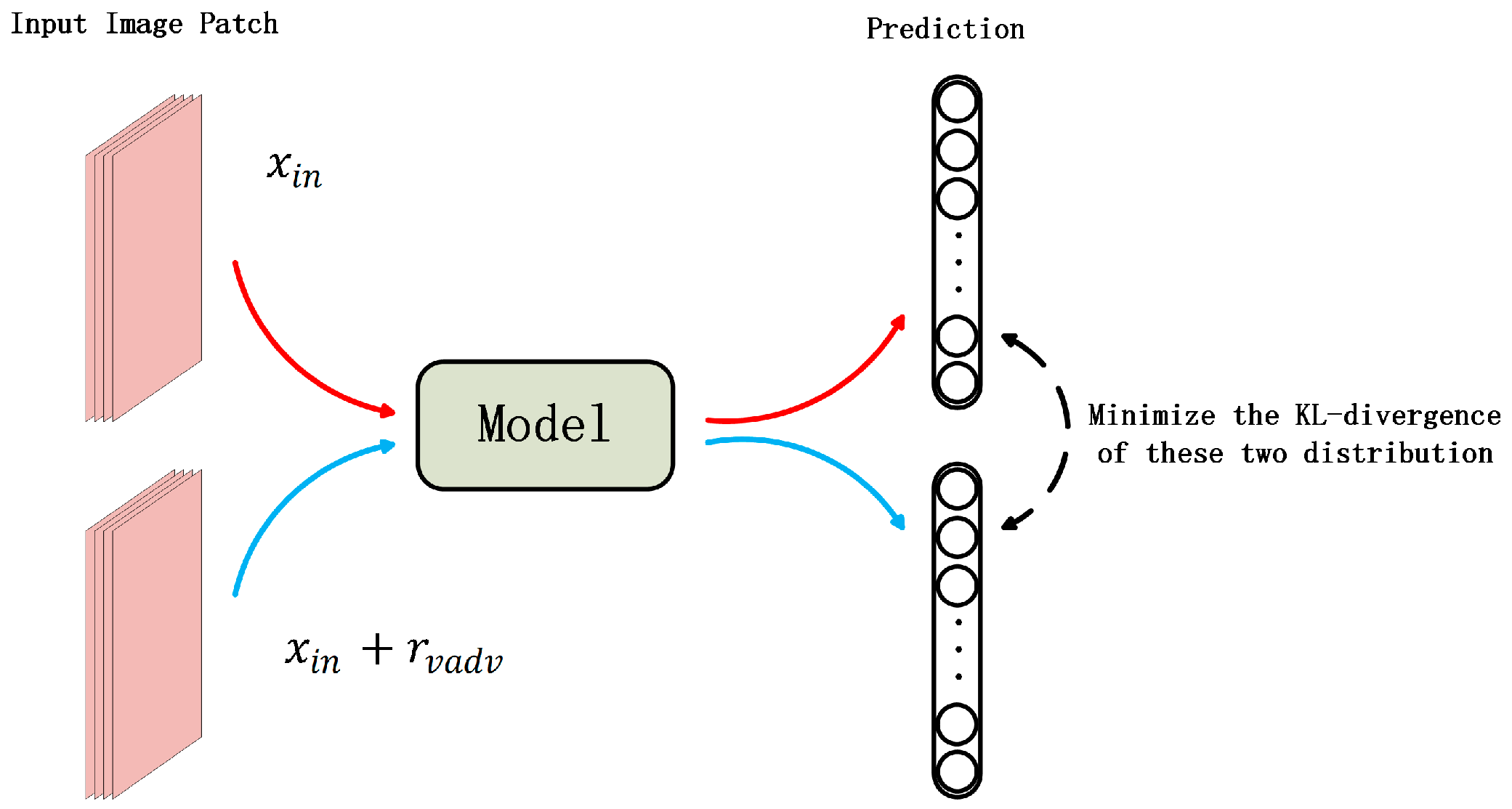
Applying deep models to small size dataset often risks overfitting, which degrades the performance of the models during validation. Virtual adversarial training (VAT) is proposed to relieve the negative influence of overfitting and strengthen the robustness of models by making models be insensitive to virtual adversarial disturbance. A brief implementation method and the solution to virtual adversarial disturbance are presented in this subsection. The main idea of the VAT is depicted in Figure 4.
Virtual adversarial training is derived from adversarial training proposed by Reference [37]. The loss term of the original adversarial training is presented as follows:
where indicates the real label output distribution given by the corresponding input sample . denotes the distribution of model output given by adversarial disturbed input . represents the Kullback–Leibler divergence. The aim of this loss term is to make this output distribution be close to the real output distribution. However, this distribution is usually unknown. In [37], is simplified by the one-hot label vector , which cannot be applied to unlabeled dataset. VAT [35,36] adopts the current estimation of the model output distribution to approximate , i.e.,
where is the model parameters and represents the current state of model parameters. denotes the virtual adversarial disturbance given by input and model parameters . [35,36] also proposes a fast computation method of . We denote as for simplification purpose. Assume the existence of the first and second order derivatives of with respect to always hold. As reaches its minimum value when , we can derive that the first order derivative of with respect to equals 0 at . Thus, the second order Taylor expansion of is shown as follows:
where denotes the Hessian matrix of . Based on the assumption given above, will be close to the first dominant eigenvector of with amplitude .
where is the direction vector of . By using power iteration and finite difference method, the direction vector of this eigenvector can be approximated iteratively using the equation as follows:
where is a random vector before the first iteration and gets updated iteratively for times, is a small definite number used in finite difference method. In this paper, 1-time iteration is used to fit the eigenvector.
3. Proposed Method
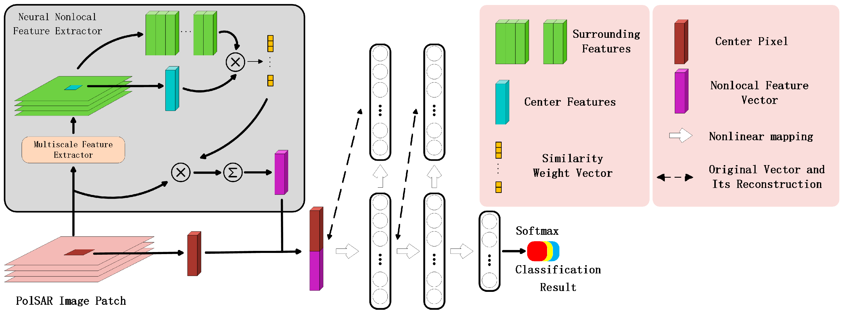
In this paper, an end-to-end deep neural network called NNSSAE is proposed for PolSAR image classification. The proposed model contains two types of deep modules, i.e., a multiscale similarity based feature extractor and a stacked sparse autoencoders (SSAE). The feature extractor, named as neural nonlocal feature extractor (NNFE), is composed of feedforward neural networks and calculates the weighted sum of the PolSAR image patch. SSAE takes the output of NNFE as input to project original pixel features and nonlocal features into high dimensional latent space. Softmax classifier is introduced to conduct the final classification task. Meanwhile, we introduce VAT regularization term in the loss function to relieve the overfitting and to achieve higher generalization ability. The whole framework of the model is depicted in Figure 5.
3.1. Input Feature Preparation
Every pixel in PolSAR data is represented as a scattering matrix that indicates the polarimetric scattering characteristics of the ground objects. The matrix is given by
where is the element that is horizontal transmitting and vertical receiving polarized, and the definition of the other three elements can be derived in a similar manner. Under the assumption that , the scattering vector is given by
Followed by Reference [38], a covariance matrix of an -look image is represented by
where denotes the -th one-look sample, and represents the Hermitian transpose. From [38], we can derive the coherency matrix from Equation (21).
Since the coherency matrix is known to be a Hermitian matrix, we simply takes the upper triangular part of the matrix as the input of our model. To avoid introduce complex number into our model, we separate the real and imagine part of these complex elements, i.e., we have .
3.2. Neural Nonlocal Feature Extractor
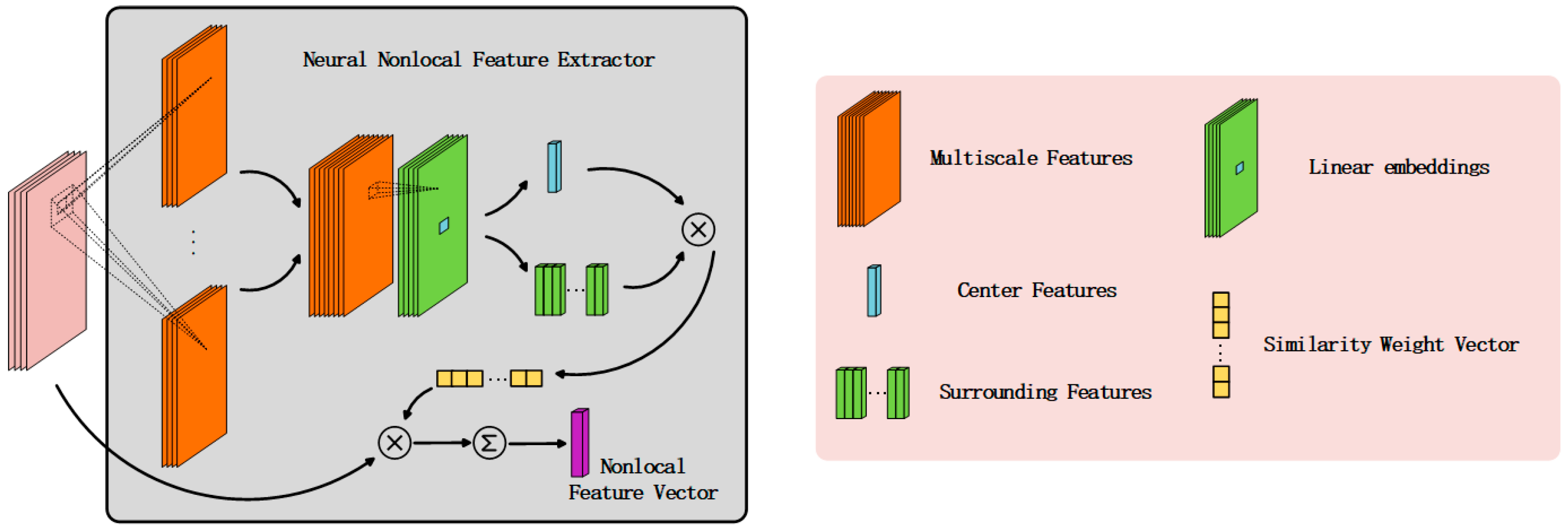
Nonlocal methods generally share the same core concept that calculates weighted sum of the surrounding pixels to extract the nonlocal features of the center pixel. The difference between them is the different weight calculation criterions. NNFE adopts parameterized model to reveal the spatial features and uses the dot product of the feature vectors of surrounding pixels and the center pixel as its weight calculation criterion. The parameters are updated by back-propagation [39] algorithms, which relies on mining the information buried in data rather than careful selection adopted by hand-crafted algorithms. The structure of the NNFE is shown in Figure 6.
Before neural nonlocal operation, a multiscale feature extraction operation is implemented on the original image patch to relieve the degradation effect accompanied with speckle noise. Inspired by NLN, we use dot product rather than the variants of Euclidean distance, for the computation complexity of the former one is negligible compared with the latter one.
The multiscale feature extraction operation utilizes , and convolutional kernels, which is inspired by the Inception block [40]. These kernels of various scales can both effectively capture the discriminative features and substitute the complicated introduced by ANFE. The output of the kernels represent the characteristics of the pixel themselves, which provides the functionality like a soft version of . Then, features of different scales are concatenated to constitute the input of the nonlocal operation block, . Through linear embedding layer, the feature of pixel and the set of pixels’ features in the central window are used to calculate the corresponding weight set by the exponential dot product:
where denotes the normalization factor. The weight set is then used for weighted sum feature calculation. Apparently, the nonlocal feature vector has the same dimension with the original pixel vector .
Considering that NNFE is fully parameterized thus need to be optimized, and SSAE need initial feature vector to conduct unsupervised pre-training, an auxiliary classifier based on Softmax regression is introduced to train NNFE to reach a proper initial state.
The main improvement of the nonlocal blocks compared with traditional neural networks is that it is capable with analyzing the pairwise relationship of all the pixels in the feature maps. By introducing the weights based on adaptive similarity calculation, both NLN and NNFE will have larger vision field and be enabled to extract nonlocal features. The differences between the nonlocal operation introduced in NLN and the nonlocal operation proposed in this paper could be summarized in two folds: First, the similarity calculation of the NNFE focuses on the center pixel of the nonlocal feature maps, rather than every pixel in the feature maps under the circumstance of NLN. Second, the nonlocal feature vector extracted by NNFE is simply calculated by applying the weighted sum on the original central window, for this could make the nonlocal feature vector have similar distribution compared with the feature vector of the original pixel.
3.3. Stacked Sparse Autoencoders
A two-layer SSAE is implemented to map the original and the nonlocal features into latent space and finally conduct classification on optimized features using a Softmax classifier.
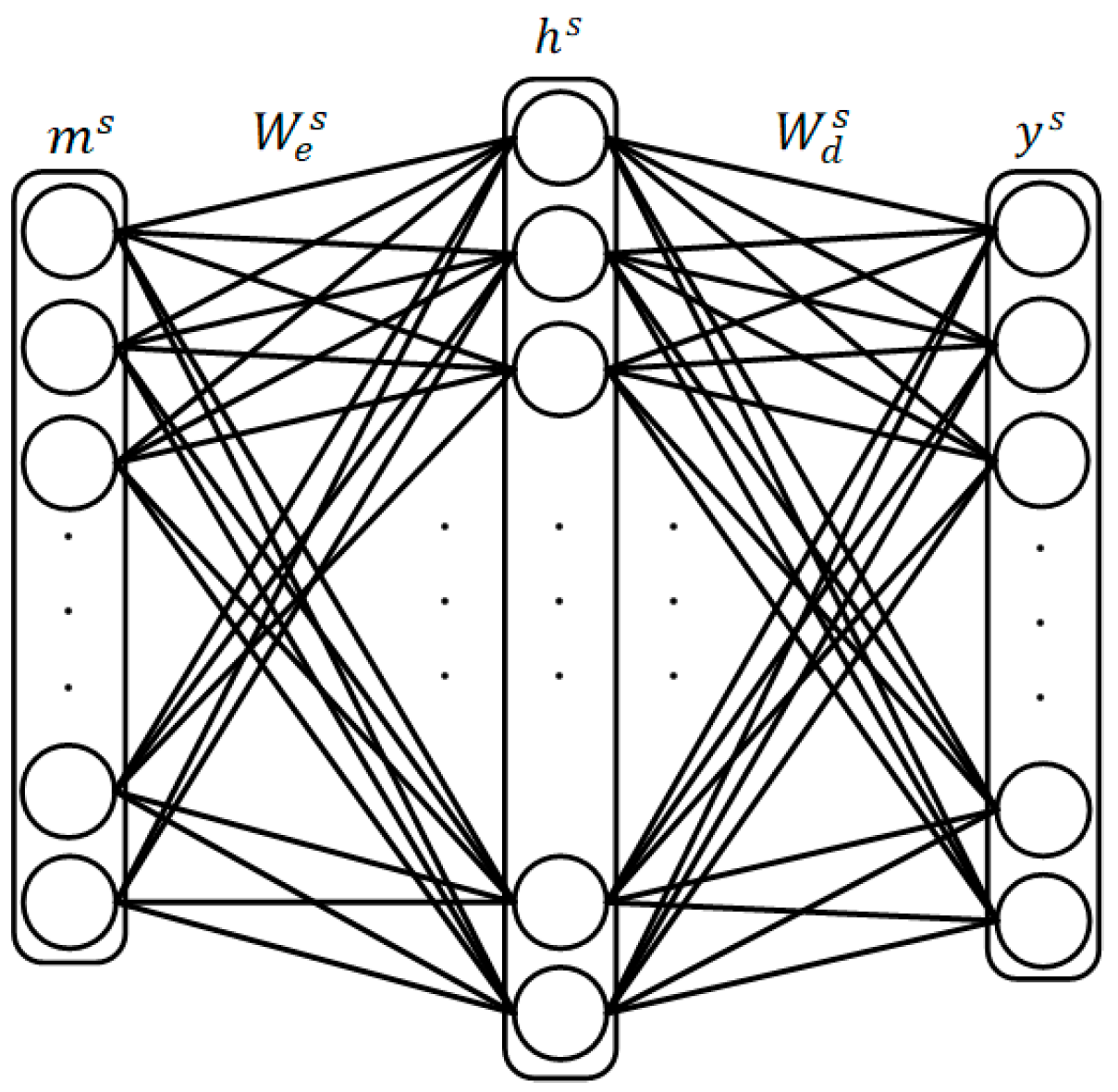
The training procedure of SSAE contains two steps: Pretraining and fine-tuning. Assume that the SSAE model is composed of autoencoders. The structure of Autoencoder is shown in Figure 7. At the pre-training stage, the input of the -th autoencoder is denoted as . This input is encoded as a hidden representation , and then is decoded as a reconstructed representation .
where , are the weight matrix and bias vector of the encoder, and , are the weight matrix and bias vector of the decoder. represents a nonlinear function, here we use the sigmoid function which has the expression of . The loss function of this sparse autoencoder is shown as follows:
where is the number of the training samples in a mini-batch, represents the scaling factor of the weight regularization term, and is a scaling factor controlling the strength of the sparse penalty. is the sparse parameter usually holding a small value. denotes the averaged response on this specific mini-batch of the -th unit in the -th autoencoder, and is the number of the units in the -th autoencoder. represents the Kullback–Leibler divergence of two distribution. Minimizing the sparse penalty term in the loss function will make the response of units in the hidden layer be close to zero. When the -th autoencoder is trained, its hidden representation will become the input of the -th autoencoder , noted that the input of the first autoencoder is the input of the SSAE.
When the last autoencoder finishes its pre-training process, a Softmax classifier is connected after the hidden representation of the last autoencoder to predict the label distribution of every sample. The expression of the Softmax classifier is:
where is the number of categories contained in the dataset.
3.4. Loss Function in the Fine-Tuning Stage and the VAT Regularization Term
At the fine-tuning stage, virtual adversarial training and supervised cross-entropy loss are combined together to guide the back-propagation algorithm to optimize the parameters of the model. We denote dataset as and the set of samples perturbed by VAT as . The Loss function in the fine-tuning stage is shown in Equation (28).
The first term is the cross-entropy term, which represents the difference between the distribution of the model prediction performed on the training samples and the distribution of the corresponding labels. In Equation (28), represents the one-hot label vector and represents the model prediction distribution. This term aims to make the predictions be close to the labels, thus yields to better accuracy performance. The second term is the VAT regularization term, which denotes the flatness of the model prediction distribution in the high dimensional latent space around each training sample. The purpose of this term is to smooth the output distribution around input data, and make the model more robust.
The calculation of is concluded in Algorithm 1.
| Algorithm 1. Calculation of Virtual Adversarial Training Disturbance |
| Input: Mini-batch size , dataset ; |
| Step 1: Randomly select samples dataset to construct a mini-batch. |
| Step 2: Sample unit vectors from an i.i.d Gaussian distribution. |
| Step 3: Calculate using Equation (16) and Equation (17) with respect to on on each sample. |
| Output: Virtual adversarial disturbance . |
3.5. Training Strategy
Algorithm 2 summarizes the details in training processes. The training procedure mainly contains three stages. First, in order to provide coarse nonlocal features to SSAE, the NNFE is pre-trained using training samples in a supervised manner. Only samples in the training set are used in this stage. Then SSAE takes both the center pixels and the initialized nonlocal feature vectors as input and extracts their latent information by unsupervised layerwise reconstruction training. Finally, the whole framework is fine-tuned supervisedly using the training samples with the regularization of the VAT.
| Algorithm 2. The training strategy of NNSSAE-VAT |
| Input: PolSAR Image, label map; |
| Step 1: Select of samples per category from the labeled samples to construct training set. |
| Step 2: Initialize all trainable parameters . |
| Step 3: Use the auxiliary classifier to pretrain the NNFE with sample-label pairs by BP Algorithm. |
| Step 4: For the -th autoencoder in autoencoders: Train the autoencoder to reconstruct the input , minimize the L2-difference between the input and the reconstructed result . |
| Step 5: Use the main classifier to fine-tune the whole network with virtual adversarial training term in the loss function. |
| Output: The trained model , prediction map. |
4. Experiments
In this section, three real PolSAR images are utilized to verify the effectiveness of the proposed method. The first dataset covering Flevoland, Netherlands, is obtained by AIRSAR platform in 1989. The second dataset is the C-band Benchmark dataset acquired by AIRSAR platform in 1991, covering another part of Flevoland. The third dataset is the full-polarimetric L-band image covering Foulum, Denmark, which is obtained by EMISAR platform in 1998. To restrain the negative effects brought by speckle noise, all these three PolSAR image are preprocessed by refined Lee filtering [41], and the window size of the filter is set to 5 for fair comparison. We use python/Tensorflow to conduct the experiments, which are implemented on a computer with Inter(R) Core™ i7-4790K CPU, 16G RAM and NVIDIA GTX960 GPU.
The proposed NNSSAE-VAT is compared with four relevant methods, including SSAE [23], SSAE-LS [26], SRDNN [30], ANSSAE [32]. Since all methods are AE-based classification models, their hyperparameters are set as same as the original papers, respectively. The metrics used for comparison include overall accuracy (OA), average accuracy (AA), and Kappa coefficient ().
4.1. Experimental Settings
4.1.1. Networks Architecture Settings and Analyses
For SSAE and SSAE-LS, the number of the hidden units in the two hidden layers are both set to 300. For SRDNN, the two hidden layers are set to have 150 and 40 units. As for ANSSAE, it is set to have five layers and its detailed configuration for each dataset will be illustrated in the following subsections, respectively. The Softmax classifier is connected after the final hidden layer to conduct classification task.
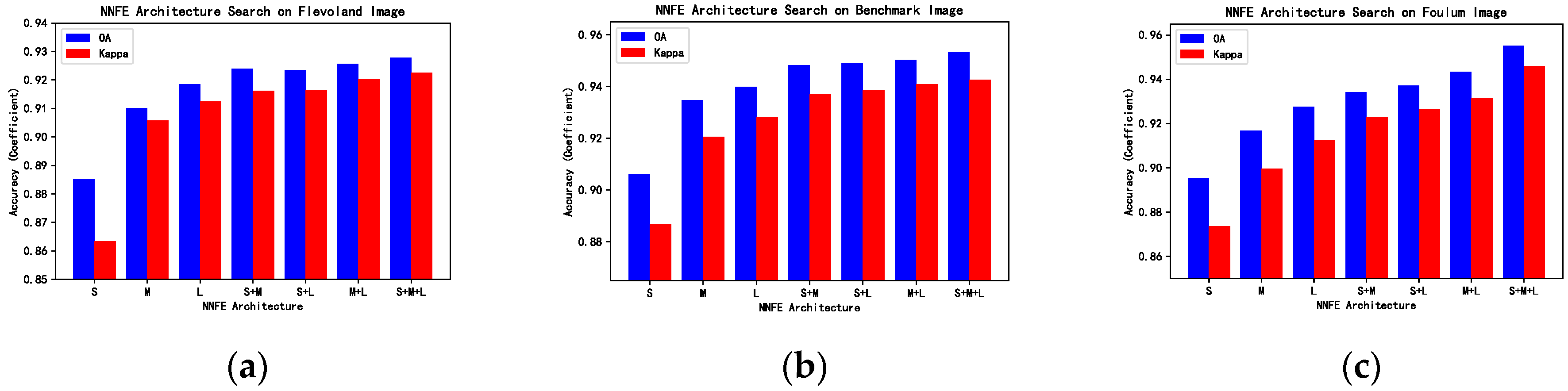
For autoencoder-based PolSAR image classification models, the classification accuracy depends on the effectiveness of their feature extractors. Thus, the architecture of NNFE should be carefully designed in order to fully utilize the strong representation capability of SSAE and achieve better performance. To this end, we determine the architecture of NNFE by conducting experiments on all the three PolSAR data used in this paper. During this experiment, only the auxiliary classifier is used, which is connected directly to the output of the NNFE. NNFE contains two parts of parameterized layers, i.e., the multiscale feature extractor layer and the linear embedding layer. The number of kernels in feature extractor layer is set to 30 and the number of kernels in linear embedding layer is set to 40. The result of this experiment is shown in Figure 8.
In Figure 8, ‘S’, ‘M’, and ‘L’ represents kernels of scale , , and , respectively. Besides, the symbol ‘+’ indicates the concatenation of multiple scales. From the results, it is apparent that the NNFE with kernels of all three scales outperforms other variants. In general, NNFEs with kernels of multiple scales have better performance compared with NNFEs with kernels of single scales. Combined with kernels of scale , the ‘S+M+L’ module achieves higher accuracy results compared with original ‘M+L’ module. One possible reason for this is that the kernels represent features of the pixels themselves, which act like a soft version of . To prove the robustness of the proposed model, we fix all the hyper-parameters to constant values during the experiments described in Section 4.2, Section 4.3 and Section 4.4. The number of kernels in multiscale feature extractor layer is set to 30 for , and kernels, and the number of kernels in linear embedding layer is set to 40. We set the SSAE part to , , , , and each layer has 220 hidden units throughout the experiments.
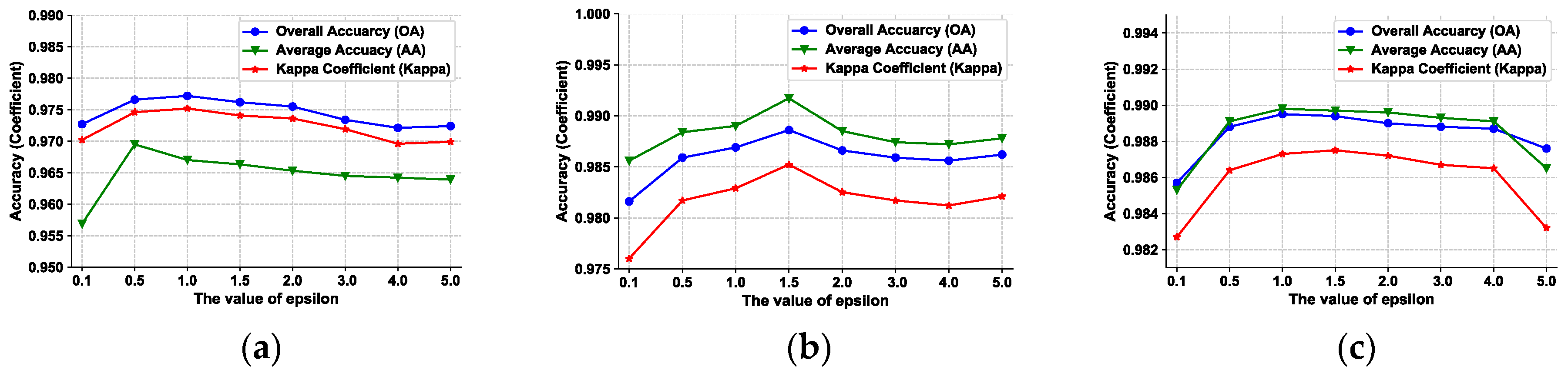
4.1.2. Parameter Settings for Virtual Adversarial Regularization Term
According to [35,36], the essential parameters of VAT are regularization weight , perturbation length , a small value and the number of the power iteration . In the original papers, the value of is fixed to , for it is merely a small value used in finite differential method, which is a numerical calculation approach. The parameter represents the number of power iteration is performed on the random vector to make it fit the most significant eigenvector of the Hessian matrix . No significant improvement is observed when we pick as values larger than 1, for which we fix the value of to 1. The regularization weight denotes the importance of the VAT term compared with the cross-entropy term in the loss function and the perturbation length is the core parameter controlling the length of VAT perturbation .
Considering that the intention of combining VAT with NNSSAE is to regularize the model and relieve the negative effects of overfitting, we simply set and search for to achieve the best results of the proposed model. The experimental results of the datasets with a different value of are shown in Figure 9.
From the results we can derive that when belongs to the model is capable to achieve promising performance. We also observe that when is smaller than 0.5 and is larger than 4.0, the performance is degraded. When is smaller than 0.5, the regularization effect is limited because the perturbed data points are too close to the original data points; This means the regions around data points are too small to make the corresponding output distribution smooth. When is larger than 4.0, the region around data points are too large and may unexpectedly include data points of other classes. Hence, we suggest using a general range of from 0.5 to 3.0 for NNSSAE-VAT model.
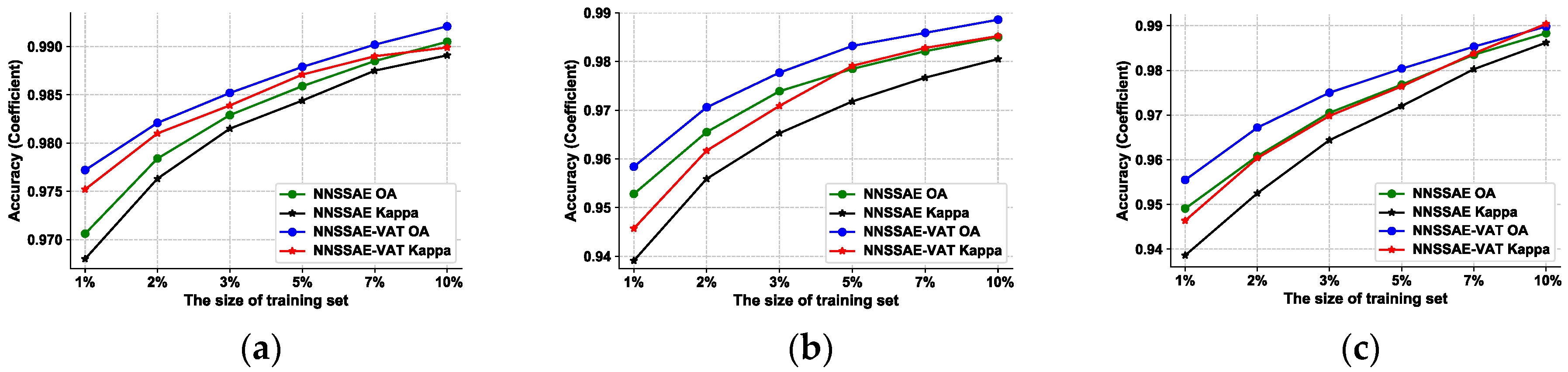
4.1.3. Influences of Different Sizes of the Training Set
We conduct experiments that test different sizes of training set for all three datasets. The sizes we chosen are 1%, 2%, 3%, 5%, 7%, and 10%. The results are shown in Figure 10. We find that Flevoland dataset is kind of ‘easier’ compared with the C-band Benchmark dataset and Foulum dataset, because in general Flevoland dataset doesn’t have classes that are easily confused with each other, although it does have the largest number of classes. For evidence, from Table 1, Table 2 and Table 3, we can find that the accuracy of SSAE is 89.75% in the case of Flevoland dataset only using 1% labeled samples, while the accuracies become 89.65% and 90.97% using 10% labeled samples when SSAE is applied to the other two dataset. For this reason, we think 1% is good enough to be the size of the training set of Flevoland dataset, and we set the size of the training set of the other two datasets to 10%.
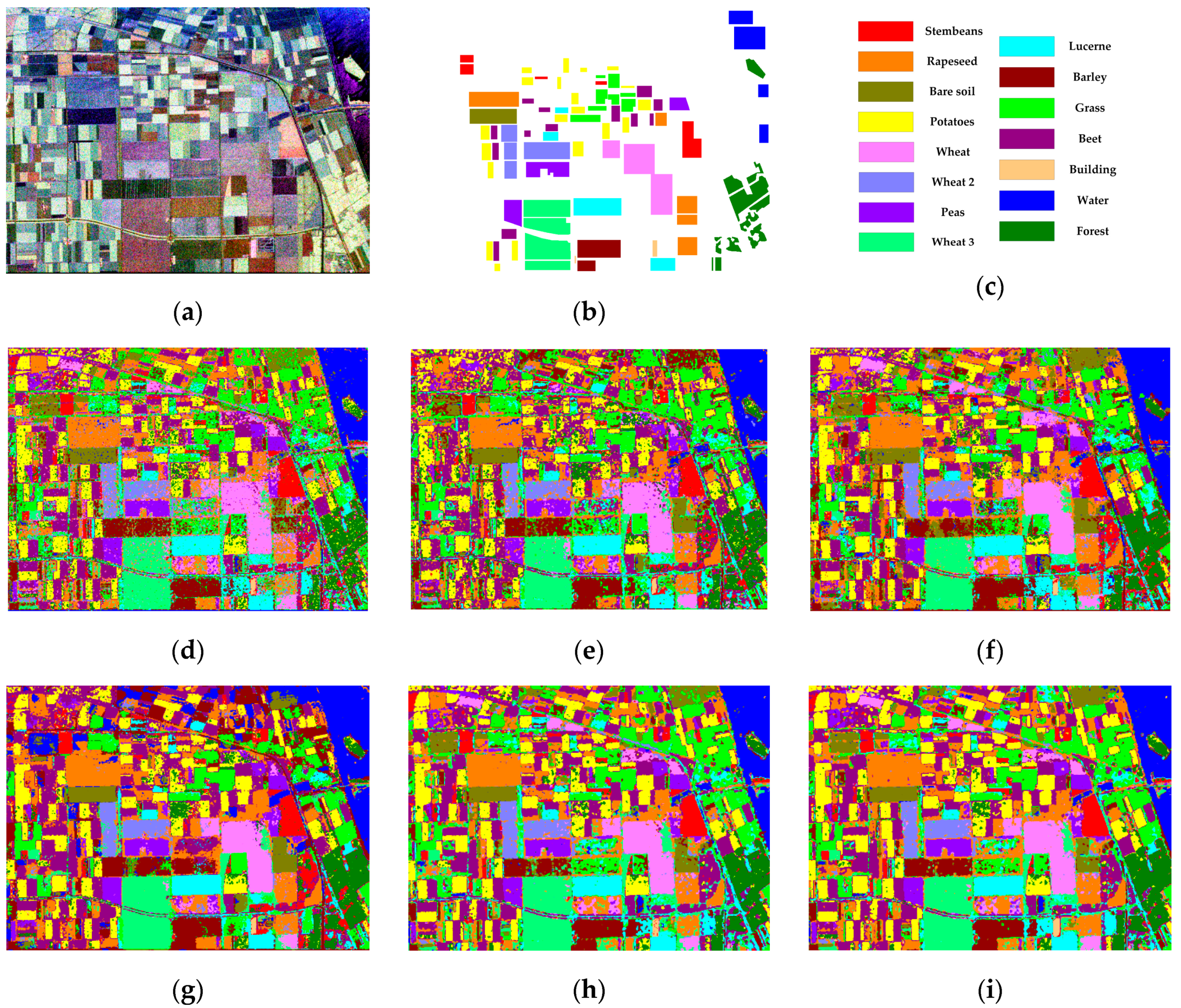
4.2. Flevoland Dataset
The Flevoland image has 750 × 1024 pixels, which are labeled with 15 categories. The number of labeled pixels is 161,327. Figure 11a shows the Pauli-RGB pseudo color image, Figure 11b,c shows its corresponding ground truth, and Figure 11d–i are classification results. In the experiment, 1% labeled samples are randomly selected to construct training set, and the rest is used for testing. For SRDNN, the number of superpixels is set to 8000. For ANSSAE, the parameter controlling the vector is set to 0.0005, and the hidden units number of each layer is set to 180.
The accuracy performance is reported in Table 1, from which we can find that the NNSSAE and NNSSAE-VAT achieve higher accuracy than other methods. In the absence of spatial information, the SSAE are highly sensitive to the negative effect brought by speckle noise, especially when the size of training set is limited. The SSAE-LS significantly improves the classification performance, for involving pixels surrounding the center pixel makes training samples become more discriminable. Nonlocal methods further improve the accuracy and reduce misclassified spot in the large homogeneous regions. The SRDNN clusters pixels in the original PolSAR image using the intensity and the spatial distance of pixels. However, in other words, this means the performance of the model is essentially dependent the segmentation of superpixels. The ANSSAE achieve better performance compared with SRDNN, for it extracts nonlocal information in a more precise pixel-wise manner.
The proposed NNSSAE shows even better accuracy performance than the two previously mentioned nonlocal methods. Using deep neural embedding features, NNSSAE extracts more robust nonlocal information for every pixel in the image, which is proved to have better discriminative capability than ANSSAE. Furthermore, the proposed NNSSAE-VAT improves the accuracy about 0.6% compared with NNSSAE, which proves the effectiveness of the VAT regularization under the situation that the amount of training data is limited.
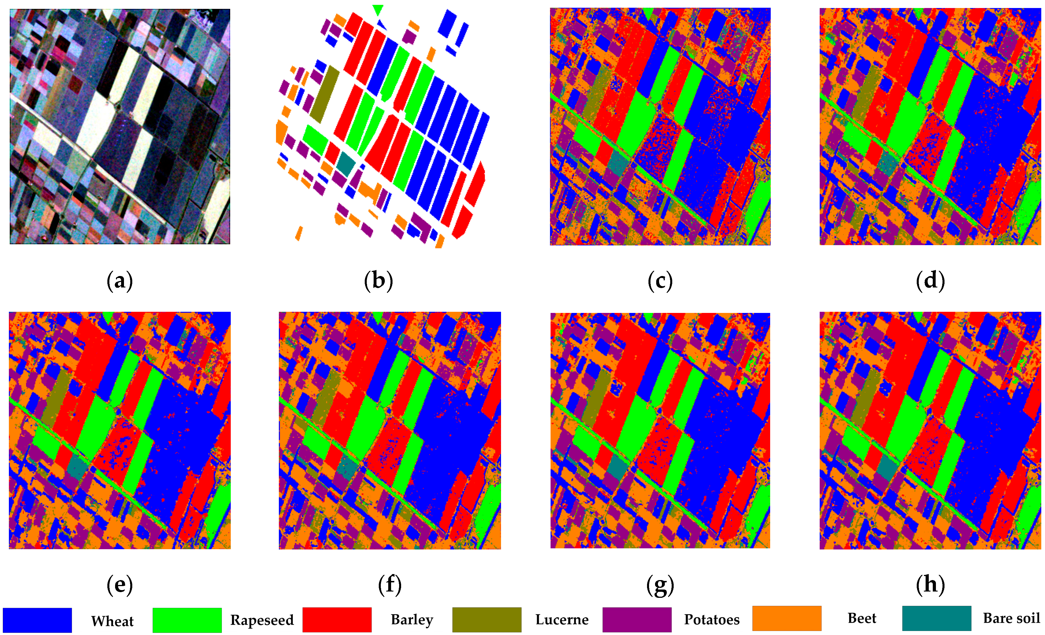
4.3. Benchmark Dataset
The C-band Benchmark dataset is 700 750 with 7 labeled categories. The number of labeled pixels is 203,223, which indicates that this dataset has the smallest image size but has the largest number of labeled samples. Figure 12a shows the Pauli-RGB pseudo color image and Figure 12b shows its corresponding ground truth. In the experiment, 10% labeled samples are randomly selected to construct training set, and the rest is used for testing. For SRDNN, the number of superpixels is set to 6500. For ANSSAE, is set to 0.0005, and the hidden units number of each layer is set to 150.
The classification performance is presented in Table 2, and the corresponding classification results are shown in Figure 12c–h, respectively. From Figure 12c, it is apparent that SSAE misclassified a considerably large part of barley into wheat. Besides, the classification result of Lucerne is quite confused with Beet, and the pea is highly confused with potato. The result of SSAE indicates that the spatial information is crucial when classes that can merely be discriminated by analyzing the context of spatial regions. The SSAE-LS significantly improved the accuracy performance, while the result is inferior to nonlocal methods, for its vision field size is still insufficient to capsule more discriminative features and it uses fixed isotropic decaying weights instead of adaptive feature-driven weights. The ANSSAE achieves better accuracy than SRDNN, for the reason that rather than calculating averaged value in a superpixel, ANSSAE calculates similarity-based averaged value for each pixel. The NNSSAE obtains the best result among other methods used for comparison, which shows that the nonlocal features extracted by NNFE are more efficient. Regularized by VAT, the NNSSAE-VAT further improves the performance, indicating that VAT is capable to make neural networks become more robust.
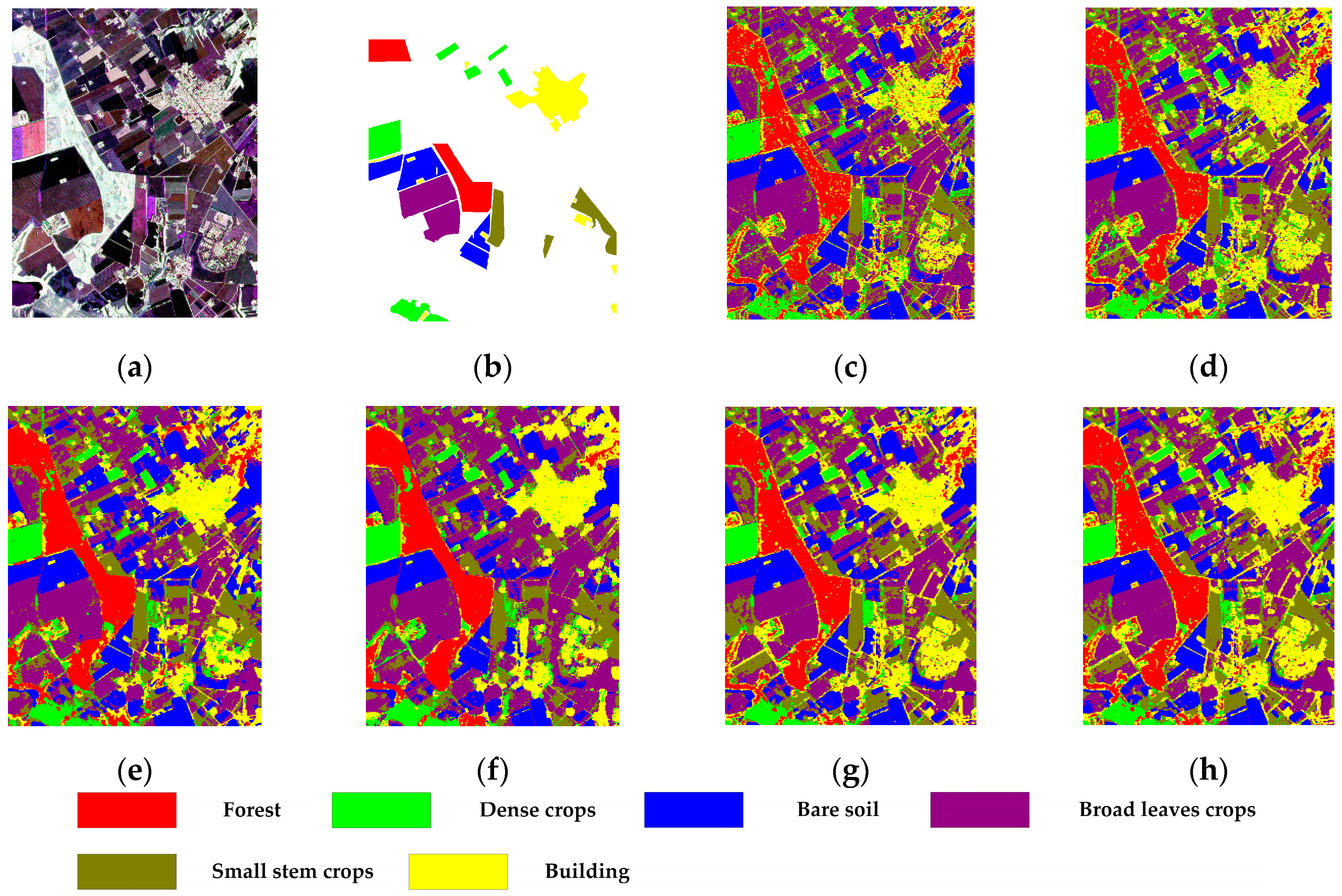
4.4. Foulum Dataset
The Foulum image has pixels, which are labeled with 6 categories. The number of labeled pixels is 169,386. Figure 13a shows the Pauli-RGB pseudo color image and Figure 13b shows its corresponding ground truth. In the experiment, 10% labeled samples are randomly selected to construct training set, and the rest is used for testing. The experiment results are shown in Figure 13c–h and Table 3. In Table 3, dense crops, broad leaves crops and small stem crops are denoted as D.c, B.l.c, and S.s.c, respectively. For SRDNN, the number of superpixels is set to 9000. For ANSSAE, the parameter is set to 0.00055, and the hidden units number of each layer is set to 80.
As is shown in Table 3, the proposed NNSSAE model achieves higher overall accuracy than the methods, which do not use NNFE as their feature extractor. Noted that the SSAE takes the original image pixels as input, its performance is considerably degraded by the speckle noise. From the classification result shown in Figure 13c it can be observed that the buildings, forest and some part of dense crop can be easily confused without the presence of spatial information. As a result of involving local spatial information, the SSAE-LS performs better than the SSAE, improve the OA about 5%. Furthermore, nonlocal methods extract spatial features based on various similarity calculations. Besides, NNSSAE and ANSSAE show comparable results, which indicate the robustness of the NNSSAE, for it can achieve competitive performance without carefully selecting parameters. With the regularization of the VAT, the NNSSAE-VAT further improves the OA and AA compared with the NNSSAE.
5. Discussion
Feature extractor and classifier are two essential modules for PolSAR image classification. Efficient feature extractor and robust classifier have a strong link with good classification performance. The proposed NNSSAE-VAT method uses NNFE to capsule multiscale spatial features and use similarity based weighted sum to calculate the discriminative nonlocal feature vector without manually designed expert parameters. The experimental results have shown the effectiveness of NNFE. SSAE is utilized as the classifier of the proposed method, for it can project the input features into deep latent space and achieve good classification performance.
VAT term is also introduce in the proposed method to regularize the model, because the strong capability to fit training data of deep learning models can also cause overfitting when the training data is insufficient. This circumstance is consistent with PolSAR image classification. For evidence, in Figure 10, we notice that applying VAT will achieve relatively larger accuracy improvement when the size of the training set is small. Another significance of applying VAT to NNSSAE is that we can achieve similar performance with smaller size of training set using same architecture of the model, which could be derived in Figure 10 as well. This means VAT could further reduce the workload of manually labeling the ground objects.
The time consumption during training procedures for all six method are shown in Table 4, where “Prep” denotes the time used for pre-processing, “Train” denotes the training time, and “Total” denotes the time used during the whole training procedure.
From Table 4, we could also find that the time required by the pre-processing stage of the ANSSAE model is quite long, which could be a limitation in real applications. The training time of the proposed NNSSAE and NNSSAE-VAT are higher compared with other methods, because the former two models have neural network based feature extractors, which need to be trained. Moreover, applying VAT to NNSSAE introduces more time in training procedure, for implementing VAT will increase the amount of computation. More competent structure of NNFE and more efficient calculation algorithm for the virtual adversarial perturbation term could be further investigated in the future. Considering the advantages of NNFE, we also plan to combine the NNFE with fully convolutional network (FCN) [42] to further improve the classification accuracy and reduce the time consumption in our future work.
6. Conclusions
In this paper, we propose a method called NNSSAE-VAT for PolSAR image classification. The NNSSAE-VAT mainly contains three parts: The neural nonlocal feature extractor (NNFE), the SSAE, and the virtual adversarial training regularization terms. The NNFE uses a neural network calculating pairwise similarity between each pixel and its surrounding pixels in a pairwise manner as the filtering weights to extract nonlocal features. The SSAE takes the combination of the original pixel and its neural nonlocal features to perform classification and the VAT regularization term is introduced to make the model be more robust. The experimental results derived from three real PolSAR images shows that the proposed method achieves better results compared with previous methods.
Author Contributions
All the authors made important contributions to this work. R.W. designed the model. R.W. conceived the experiments and analyzed the results. R.W. wrote the paper and Y.W. provided instruction and advice for the preparation of the paper.
Funding
This research was funded by Ministry of Science and Technology of the People’s Republic of China, under the National Key Research and Development Program, Grant number 2017YFB0503001.
Conflicts of Interest
The authors declare no conflict of interest.
References
- Hajnsek, I.; Jagdhuber, T.; Schon, H.; Papathanassiou, K.P. Potential of Estimating Soil Moisture under Vegetation Cover by Means of PolSAR. IEEE Trans. Geosci. Remote Sens. 2009, 47, 442–454. [Google Scholar] [CrossRef]
- Jiao, X.; Kovacs, J.M.; Shag, J.; McNairn, H.; Walters, D.; Ma, B.; Geng, X. Object-oriented crop mapping and monitoring using multi-temporal polarimetric RADARSAT-2 data. ISPRS J. Photogramm. Remote Sens. 2014, 96, 38–46. [Google Scholar] [CrossRef]
- Singh, G.; Yamaguchi, Y.; Boerner, W.M.; Park, S.E. Monitoring of the March 11, 2011, off-Tohoku 9.0 earthquake with super-tsunami disaster by implementing fully polarimetric high-resolution POLSAR techniques. Proc. IEEE 2013, 101, 831–846. [Google Scholar] [CrossRef]
- Chen, Q.; Li, L.; Jiang, P.; Liu, X. Building collapse extraction using modified freeman decomposition from post-disaster polarimetric SAR image. In Proceedings of the 2016 IEEE International Geoscience and Remote Sensing Symposium (IGARSS), Beijing, China, 10–15 July 2016; pp. 5769–5772. [Google Scholar]
- Liu, C.; Gierull, C.H. A new application for PolSAR imagery in the field of moving target indication/ship detection. IEEE Trans. Geosci. Remote Sens. 2007, 45, 3426–3436. [Google Scholar] [CrossRef]
- Wang, L.; Scott, K.A.; Xu, L.; Clausi, D.A. Sea ice concentration estimation during melt from dual-pol SAR scenes using deep convolutional neural networks: A case study. IEEE Trans. Geosci. Remote Sens. 2016, 54, 4524–4533. [Google Scholar] [CrossRef]
- Lee, J.-S.; Grunes, M.R.; Ainsworth, T.L.; Du, L.-J.; Schuler, D.-L.; Cloude, S.R. Unsupervised classification using polarimetric decomposition and the complex Wishart classifier. IEEE Trans. Geosci. Remote Sens. 1999, 37, 2249–2258. [Google Scholar]
- Lee, J.S.; Grunes, M.R.; Pottier, E.; Ferro-Famil, L. Unsupervised terrain classification preserving polarimetric scattering characteristics. IEEE Trans. Geosci. Remote Sens. 2004, 42, 722–731. [Google Scholar]
- Zhang, L.; Zou, B.; Zhang, J.; Zhang, Y. Classification of Polarimetric SAR Image Based on Support Vector Machine Using Multiple-component Scattering Model and Texture Features. EURASIP J. Adv. Signal Process. 2010, 2010, 1–9. [Google Scholar] [CrossRef]
- Lardeux, C.; Frison, P.L.; Tison, C.; Stoll, B.; Fruneau, B.; Rudant, J.-P. Support vector machine for multifrequency SAR polarimetric data classification. IEEE Trans. Geosci. Remote Sens. 2009, 47, 4143–4152. [Google Scholar] [CrossRef]
- Zhang, L.; Sun, L.; Zou, B.; Moon, W. Fully polarimetric SAR image classification via sparse representation and polarimetric features. IEEE J. Sel. Top. Appl. Earth Observ. Remote Sens. 2014, 8, 3923–3932. [Google Scholar] [CrossRef]
- Feng, J.; Cao, Z.; Pi, Y. Polarimetric contextual classification of PolSAR images using sparse representation and superpixels. Remote Sens. 2014, 6, 7158–7181. [Google Scholar] [CrossRef]
- Du, P.; Samat, A.; Waske, B.; Liu, S.; Li, Z. Random Forest and Rotation Forest for fully polarized SAR image classification using polarimetric and spatial features. J. Photogramm. Remote Sens. 2015, 105, 38–53. [Google Scholar] [CrossRef]
- Cloude, S.R.; Pottier, E. An entropy based classification scheme for land applications of polarimetric SAR. IEEE Trans. Geosci. Remote Sens. 1997, 35, 68–78. [Google Scholar] [CrossRef]
- Freeman, A.; Durden, S. A three-component scattering model for polarimetric SAR data. IEEE Trans. Geosci. Remote Sens. 1998, 36, 963–973. [Google Scholar] [CrossRef]
- Wu, Y.; Ji, K.; Yu, W.; Su, Y. Region-based classification of polarimetric SAR images using Wishart MRF. IEEE Geosci. Remote Sens. Lett. 2008, 5, 668–672. [Google Scholar] [CrossRef]
- Xie, W.; Xie, Z.; Zhao, F.; Ren, B. POLSAR Image Classification via Clustering-WAE Classification Model. IEEE Access. 2018, 6, 40041–40049. [Google Scholar] [CrossRef]
- Fukuda, S.; Hirosawa, H. Support vector machine classification of land cover: Application to polarimetric SAR data. In Proceedings of the IEEE 2001 International Geoscience and Remote Sensing Symposium (IGARSS ’01), Sydney, Australia, 9–13 July 2001; Volume 181, pp. 187–189. [Google Scholar]
- Zhang, L.; Zou, B.; Cai, H.; Zhang, Y. Multiple-component scattering model for polarimetric SAR image decomposition. IEEE Geosci. Remote Sens. Lett. 2008, 5, 603–607. [Google Scholar] [CrossRef]
- Mallat, S.; Zhang, Z.F. Matching pursuits with time-frequency dictionaries. IEEE Trans. Signal Process. 1993, 41, 3397–3415. [Google Scholar] [CrossRef]
- Hinton, G.E.; Salakhutdinov, R.R. Reducing the dimensionality of data with neural networks. Science 2006, 313, 504–507. [Google Scholar] [CrossRef] [PubMed]
- Bengio, Y.; Lamblin, P.; Popovici, D.; Larochelle, H.; Montreal, U. Greedy layer-wise training of deep networks. Adv. Neural Inform. Process. Syst. 2007, 19, 153–160. [Google Scholar]
- Xie, H.; Wang, S.; Liu, K.; Lin, S.; Hou, B. Multilayer feature learning for polarimetric synthetic radar data classification. In Proceedings of the IEEE Conference on International Geoscience and Remote Sensing Symposium (IGARSS), Quebec City, QC, Canada, 13–18 July 2014; pp. 2818–2821. [Google Scholar]
- Chen, W.; Gou, S.; Wang, X.; Li, X.; Jiao, L. Classification of PolSAR Images Using Multilayer Autoencoders and a Self-Paced Learning Approach. Remote Sens. 2018, 10, 110. [Google Scholar] [CrossRef]
- Hou, B.; Kou, H.; Jiao, L. Classification of polarimetric SAR images using multilayer autoencoders and superpixels. IEEE J. Sel. Top. Appl. Earth Observ. Remote Sens. 2016, 9, 3072–3081. [Google Scholar] [CrossRef]
- Zhang, L.; Ma, W.; Zhang, D. Stacked sparse autoencoder in PolSAR data classification using local spatial information. IEEE Geosci. Remote Sens. Lett. 2016, 13, 1359–1363. [Google Scholar] [CrossRef]
- Lecun, Y.; Boser, B.; Denker, J.S.; Henderson, D.; Howard, R.E.; Hubbard, W.; Jackel, L.D. Backpropagation applied to handwritten zip code recognition. Neural Comput. 2014, 1, 541–551. [Google Scholar] [CrossRef]
- Zhou, Y.; Wang, H.P.; Xu, F.; Jin, Y.Q. Polarimetric SAR Image Classification Using Deep Convolutional Neural Networks. IEEE Geosci. Remote Sens. Lett. 2016, 99, 1–5. [Google Scholar] [CrossRef]
- Zhang, Z.; Wang, H.; Xu, F.; Jin, Y.Q. Complex-Valued Convolutional Neural Network and Its Application in Polarimetric SAR Image Classification. IEEE Trans. Geosci. Remote Sens. 2017, 55, 1–12. [Google Scholar] [CrossRef]
- Geng, J.; Ma, X.; Fan, J.; Wang, H. Semisupervised Classification of Polarimetric SAR Image via Superpixel Restrained Deep Neural Network. IEEE Geosci. Remote Sens. Lett. 2017, 15, 122–126. [Google Scholar] [CrossRef]
- Buades, A.; Coll, B.; Morel, J.M. A non-local algorithm for image denoising. In Proceedings of the IEEE Computer Society Conference on Computer Vision and Pattern Recognition, San Diego, CA, USA, 20–25 June 2005; pp. 60–65. [Google Scholar]
- Hu, Y.; Fan, J.; Wang, J. Classification of PolSAR Images Based on Adaptive Nonlocal Stacked Sparse Autoencoder. IEEE Geosci. Remote Sens. Lett. 2018, 15, 1050–1054. [Google Scholar] [CrossRef]
- Wang, X.; Girshick, R.; Gupta, A.; He, K. Non-local Neural Networks. In Proceedings of the 2017 IEEE Conference on Computer Vision and Pattern Recognition (CVPR), Honolulu, HI, USA, 21–26 July 2017. [Google Scholar]
- Bishop, C.M. Pattern Recognition and Machine Learning; Springer: New York, NY, USA, 2006. [Google Scholar]
- Miyato, T.; Maeda, S.-I.; Koyama, M.; Nakae, K.; Ishii, S. Distributional Smoothing with Virtual Adversarial Training. In Proceedings of the 2016 International Conference on Learning Representations (ICLR), San Juan, Puerto Rico, 2–4 May 2016. [Google Scholar]
- Miyato, T.; Maeda, S.-I.; Ishii, S.; Koyama, M. Virtual Adversarial Training: A Regularization Method for Supervised and Semi-Supervised Learning. IEEE Trans. Pattern Anal. Mach. Intell. 2018, 1–14. [Google Scholar] [CrossRef]
- Goodfellow, I.J.; Shlens, J.; Szegedy, C. Explaining and harnessing adversarial examples. In Proceedings of the 2015 International Conference on Learning Representations (ICLR), San Diego, CA, USA, 7–9 May 2015. [Google Scholar]
- Xie, W.; Jiao, L.; Hou, B.; Ma, W.; Zhao, J.; Zhang, S.; Liu, F. POLSAR Image Classification via Wishart-AE Model or Wishart-CAE Model. IEEE J. Sel. Top. Appl. Earth Obs. Remote Sens. 2017, 10, 3604–3615. [Google Scholar] [CrossRef]
- Rumelhart, D.; Hinton, G.; Williams, R. Learning Representations by back-propagating errors. Nature. 1986, 323, 533–536. [Google Scholar] [CrossRef]
- Liu, W.; Jia, T.; Sermanet, P.; Reed, S.; Anguelov, D.; Erhan, D.; Vanhoucke, V.; Rabinovich, A. Going Deeper with Convolutions. In Proceedings of the 2015 IEEE Conference on Computer Vision and Pattern Recognition (CVPR), Boston, FL, USA, 7–12 June 2015. [Google Scholar]
- Lee, J.S. Refined filtering of image noise using local statistics. Comput. Gr. Image Process. 1981, 15, 380–389. [Google Scholar] [CrossRef]
- Long, J.; Shelhamer, E.; Darrell, T. Fully convolutional networks for semantic segmentation. In Proceedings of the IEEE Conference on Computer Vision and Pattern Recognition (CVPR), Boston, MA, USA, 7–12 June 2015; pp. 3431–3440. [Google Scholar]
Figure 1.
The diagram of the nonlocal means filtering (NLM) [31] method. The olive box, the orange box, and the brown box denote search window, central window and neighborhood window, respectively. To concisely describe the main idea of NLM, the left-top pixel and the corresponding search window is taken as an example. Different colors of pixels represent different categories of ground objects.

Figure 2.
The diagram of adaptive nonlocal feature extractor (ANFE) [32]. The olive box, the orange box and the brown box denote search window, central window, and neighborhood window, respectively. To concisely describe the main idea of ANFE, the left-top pixel in the central window and the corresponding search window is taken as an example. Different colors of pixels represent different categories of ground objects.

Figure 3.
The structure of the Nonlocal block.

Figure 4.
The training scheme of the virtual adversarial training.

Figure 5.
Framework of the proposed NNSSAE.

Figure 6.
The structure of the Nonlocal Neural Feature Extractor. Only two scales of convolutional feature extractor are shown in the figure due to limited space.
Figure 6.
The structure of the Nonlocal Neural Feature Extractor. Only two scales of convolutional feature extractor are shown in the figure due to limited space.

Figure 7.
The structure of Autoencoder.

Figure 8.
The results of NNFE architecture search conducted on (a) Flevoland dataset, (b) Benchmark dataset, and (c) Foulum dataset.
Figure 8.
The results of NNFE architecture search conducted on (a) Flevoland dataset, (b) Benchmark dataset, and (c) Foulum dataset.

Figure 9.
The influence of on (a) Flevoland dataset, (b) Benchmark dataset and (c) Foulum dataset. The alpha is set to 1.0 during these experiments.
Figure 9.
The influence of on (a) Flevoland dataset, (b) Benchmark dataset and (c) Foulum dataset. The alpha is set to 1.0 during these experiments.

Figure 10.
The influence of different sizes of the training set. (a) Flevoland dataset, (b) Benchmark dataset, and (c) Foulum dataset.
Figure 10.
The influence of different sizes of the training set. (a) Flevoland dataset, (b) Benchmark dataset, and (c) Foulum dataset.

Figure 11.
Classification results of Flevoland dataset. (a) PauliRGB image; (b) Ground truth image; (c) Label annotations (d) SSAE; (e) SSAE-LS; (f) SRDNN; (g) ANSSAE; (h) NNSSAE; and (i) NNSSAE-VAT.
Figure 11.
Classification results of Flevoland dataset. (a) PauliRGB image; (b) Ground truth image; (c) Label annotations (d) SSAE; (e) SSAE-LS; (f) SRDNN; (g) ANSSAE; (h) NNSSAE; and (i) NNSSAE-VAT.

Figure 12.
Classification results of Benchmark dataset. (a) PauliRGB image; (b) Ground truth image; (c) SSAE; (d) SSAE-LS; (e) SRDNN; (f) ANSSAE; (g) NNSSAE; and (h) NNSSAE-VAT.
Figure 12.
Classification results of Benchmark dataset. (a) PauliRGB image; (b) Ground truth image; (c) SSAE; (d) SSAE-LS; (e) SRDNN; (f) ANSSAE; (g) NNSSAE; and (h) NNSSAE-VAT.

Figure 13.
Classification results of Flevoland dataset. (a) PauliRGB image; (b) Ground truth image; (c) SSAE; (d) SSAE-LS; (e) SRDNN; (f) ANSSAE; (g) NNSSAE; and (h) NNSSAE-VAT.
Figure 13.
Classification results of Flevoland dataset. (a) PauliRGB image; (b) Ground truth image; (c) SSAE; (d) SSAE-LS; (e) SRDNN; (f) ANSSAE; (g) NNSSAE; and (h) NNSSAE-VAT.


Table 1.
Classification performance of Flevoland dataset.
| Class | SSAE | SSAE-LS | SRDNN | ANSSAE | NNSSAE | NNSSAE-VAT |
|---|---|---|---|---|---|---|
| Stembeans | 0.9536 | 0.9395 | 0.9458 | 0.9586 | 0.9837 | 0.9801 |
| Rapeseed | 0.8151 | 0.8196 | 0.9177 | 0.9613 | 0.9255 | 0.9540 |
| Bare soil | 0.9421 | 0.9577 | 0.9616 | 0.9966 | 0.9890 | 0.9922 |
| Potatoes | 0.8649 | 0.8787 | 0.9480 | 0.9237 | 0.9610 | 0.9706 |
| Wheat 1 | 0.8976 | 0.9358 | 0.9669 | 0.9764 | 0.9659 | 0.9730 |
| Wheat 2 | 0.7793 | 0.8502 | 0.8712 | 0.9524 | 0.9431 | 0.9539 |
| Peas | 0.9404 | 0.9406 | 0.9658 | 0.9878 | 0.9873 | 0.9951 |
| Wheat 3 | 0.9179 | 0.9609 | 0.9793 | 0.9901 | 0.9876 | 0.9910 |
| Lucerne | 0.9476 | 0.9633 | 0.9479 | 0.9938 | 0.9867 | 0.9889 |
| Barley | 0.9508 | 0.9178 | 0.9544 | 0.9854 | 0.9849 | 0.9860 |
| Grasses | 0.8429 | 0.8803 | 0.9469 | 0.9601 | 0.9518 | 0.9557 |
| Beet | 0.9408 | 0.8850 | 0.9512 | 0.9533 | 0.9921 | 0.9935 |
| Building | 0.8326 | 0.7892 | 0.7710 | 0.8093 | 0.8676 | 0.8054 |
| Water | 0.9745 | 0.9774 | 0.9939 | 0.9987 | 0.9947 | 0.9953 |
| Forest | 0.8756 | 0.9264 | 0.9553 | 0.9324 | 0.9629 | 0.9712 |
| OA | 0.8975 | 0.9164 | 0.9511 | 0.9665 | 0.9706 | 0.9772 |
| AA | 0.8984 | 0.9082 | 0.9385 | 0.9586 | 0.9656 | 0.9671 |
| 0.8885 | 0.9090 | 0.9468 | 0.9641 | 0.9680 | 0.9752 |
Table 2.
Classification performance of Benchmark dataset.
| Class | SSAE | SSAE-LS | SRDNN | ANSSAE | NNSSAE | NNSSAE-VAT |
|---|---|---|---|---|---|---|
| Wheat | 0.9078 | 0.9430 | 0.9638 | 0.9818 | 0.9852 | 0.9877 |
| Rapeseed | 0.9970 | 0.9950 | 0.9989 | 0.9979 | 0.9984 | 0.9997 |
| Barley | 0.8322 | 0.9242 | 0.9474 | 0.9724 | 0.9751 | 0.9785 |
| Lucerne | 0.8514 | 0.9182 | 0.9741 | 0.9596 | 0.9780 | 0.9908 |
| Potatoes | 0.9600 | 0.9731 | 0.9940 | 0.9807 | 0.9920 | 0.9978 |
| Beet | 0.7916 | 0.8958 | 0.9709 | 0.9410 | 0.9802 | 0.9883 |
| Peas | 0.8579 | 0.8955 | 0.9863 | 0.9752 | 0.9985 | 0.9991 |
| OA | 0.8965 | 0.9448 | 0.9697 | 0.9779 | 0.9850 | 0.9886 |
| AA | 0.8852 | 0.9350 | 0.9765 | 0.9727 | 0.9868 | 0.9917 |
| 0.8652 | 0.9282 | 0.9638 | 0.9713 | 0.9805 | 0.9852 |
Table 3.
Classification performance of Foulum dataset.
| Class | SSAE | SSAE-LS | SRDNN | ANSSAE | NNSSAE | NNSSAE-VAT |
|---|---|---|---|---|---|---|
| Forest | 0.9122 | 0.9595 | 0.9924 | 0.9966 | 0.9891 | 0.9904 |
| D.c | 0.8709 | 0.9688 | 0.9765 | 0.9834 | 0.9896 | 0.9910 |
| Bare soil | 0.9955 | 0.9967 | 0.9942 | 0.9967 | 0.9992 | 0.9993 |
| B.l.c | 0.9590 | 0.9828 | 0.9769 | 0.9791 | 0.9953 | 0.9945 |
| S.s.c | 0.9102 | 0.9719 | 0.9608 | 0.9670 | 0.9878 | 0.9896 |
| Buildings | 0.8140 | 0.8810 | 0.9620 | 0.9745 | 0.9697 | 0.9751 |
| OA | 0.9097 | 0.9582 | 0.9779 | 0.9838 | 0.9883 | 0.9898 |
| AA | 0.9103 | 0.9601 | 0.9771 | 0.9829 | 0.9884 | 0.9900 |
| 0.8918 | 0.9495 | 0.9733 | 0.9805 | 0.9859 | 0.9904 |
Table 4.
Time consumption of the three PolSAR image with different methods (sec).
| Methods | Flevoland | Benchmark | Foulum | ||||||
|---|---|---|---|---|---|---|---|---|---|
| Prep | Train | Total | Prep | Train | Total | Prep | Train | Total | |
| SSAE | – | 20.4 | 20.4 | – | 163.6 | 163.6 | – | 112.7 | 112.7 |
| SSAE-LS | – | 28.2 | 28.2 | – | 214.1 | 214.1 | – | 145.6 | 145.6 |
| SRDNN | 44.6 | 24.0 | 68.6 | 32.9 | 179.6 | 212.5 | 57.4 | 128.1 | 185.5 |
| ANSSAE | 1441.1 | 23.7 | 1464.8 | 1090.4 | 183.9 | 1274.3 | 1871.5 | 123.6 | 1995.1 |
| NNSSAE | – | 72.3 | 72.3 | – | 519.8 | 519.8 | – | 395.8 | 395.8 |
| NNSSAE-VAT | – | 81.8 | 81.8 | – | 593.5 | 593.5 | – | 440.7 | 440.7 |
© 2019 by the authors. Licensee MDPI, Basel, Switzerland. This article is an open access article distributed under the terms and conditions of the Creative Commons Attribution (CC BY) license (http://creativecommons.org/licenses/by/4.0/).
Share and Cite
MDPI and ACS Style
Wang, R.; Wang, Y. Classification of PolSAR Image Using Neural Nonlocal Stacked Sparse Autoencoders with Virtual Adversarial Regularization. Remote Sens. 2019, 11, 1038. https://0-doi-org.brum.beds.ac.uk/10.3390/rs11091038
AMA Style
Wang R, Wang Y. Classification of PolSAR Image Using Neural Nonlocal Stacked Sparse Autoencoders with Virtual Adversarial Regularization. Remote Sensing. 2019; 11(9):1038. https://0-doi-org.brum.beds.ac.uk/10.3390/rs11091038
Chicago/Turabian StyleWang, Ruichuan, and Yanfei Wang. 2019. "Classification of PolSAR Image Using Neural Nonlocal Stacked Sparse Autoencoders with Virtual Adversarial Regularization" Remote Sensing 11, no. 9: 1038. https://0-doi-org.brum.beds.ac.uk/10.3390/rs11091038
Note that from the first issue of 2016, this journal uses article numbers instead of page numbers. See further details here.