Cloud Detection with Historical Geostationary Satellite Sensors for Climate Applications

Abstract

Can we build stable Climate Data Records (CDRs) spanning several satellite generations? This study outlines how the ClOud Fractional Cover dataset from METeosat First and Second Generation (COMET) of the EUMETSAT Satellite Application Facility on Climate Monitoring (CM SAF) was created for the 25-year period 1991–2015. Modern multi-spectral cloud detection algorithms cannot be used for historical Geostationary (GEO) sensors due to their limited spectral resolution. We document the innovation needed to create a retrieval algorithm from scratch to provide the required accuracy and stability over several decades. It builds on inter-calibrated radiances now available for historical GEO sensors. It uses spatio-temporal information and a robust clear-sky retrieval. The real strength of GEO observations—the diurnal cycle of reflectance and brightness temperature—is fully exploited instead of just accounting for single “imagery”. The commonly-used naive Bayesian classifier is extended with covariance information of cloud state and variability. The resulting cloud fractional cover CDR has a bias of 1% Mean Bias Error (MBE), a precision of 7% bias-corrected Root-Mean-Squared-Error (bcRMSE) for monthly means, and a decadal stability of 1%. Our experience can serve as motivation for CDR developers to explore novel concepts to exploit historical sensor data.

1. Introduction

The Global Climate Observing System (GCOS) formulates a minimum decadal stability of <0.3% (for thick and low clouds) and <3% (for thin cirrus clouds) for satellite-based Cloud Fractional Cover (CFC, also known as Cloud Amount (CA)) time-series [1]. This is needed to guarantee a detectability of 0.3 W m${}^{-2}$ in cloud radiative forcing corresponding to approximately 20% of today’s anthropogenic greenhouse gas forcing [1]. This requirement can only be fulfilled with temporally-stable radiances in the retrieval scheme, traceable to an absolute standard across sensor generations. However, historical sensors often lack on-board calibration facilities, or these facilities did not function properly during the lifetime of an instrument. The consequences are temporal inhomogeneities in the Climate Data Records (CDRs) due to calibration issues, spectral differences, or acquisition time differences, which render them inappropriate for climate analysis [2]. Through the Global Space-based Inter-Calibration System (GSICS) [3,4], inter-calibration methods are now jointly developed and shared among space agencies. GSICS inter-calibration results are of unprecedented quality. The work in [5] for instance reported the correction of a 2.7 K and −2.3 K bias of the Meteosat Visible and Infrared Imager (MVIRI) on Meteosat-7 for the Water-Vapor absorption (WV) and Infrared (IR) channels, respectively, by use of the Metop-A/IASI as the reference instrument. Having calibrated radiances at hand further enables physical interpretation, the application of radiative transfer models [6], or the assimilation into numerical weather prediction or climate models [7].

For cloud detection, calibrated radiances are mostly transformed into reflectances and brightness temperatures. Their absolute values are highly informative for optically-opaque and vertically- and horizontally-extensive cloud types such as alto-stratus or nimbostratus. They are also needed to derive cloud radiative effects and cloud physical properties. For any sub-pixel or optically-thin cloud such as fair weather cumulus, low stratus, or cirrus cloud types, satellite sensors observe a mixed signal of clouds and the underlying water, ice, or land surface or another cloud layer. This is where the analysis of reflectance and brightness temperature values relative to their clear-sky counterpart becomes useful. However, the separation of cloud versus cloud-free (reference) signal has been an everlasting and key issue in satellite-based cloud detection. It can be partly circumvented by the use of unique emissivity or reflectance differences between channels. Examples are the snow/cloud separation using the 0.6–1.6-$\mathsf{\mu }$m reflectance difference [8], the cirrus detection using the 10–12-$\mathsf{\mu }$m brightness temperature difference [9], or the cloud phase separation using the 8.7–12-$\mathsf{\mu }$m brightness temperature difference [10]. Those difference tests however cannot be applied to historical GEO sensors. A CDR derived from Meteosat First Generation (MFG) and Meteosat Second Generation (MSG) data is for instance left with only three common channels. Only two of them (the broadband solar channel and the thermal infrared window channel) are useful for cloud detection. The spatial variance of single channels can potentially yield information of broken clouds or cloud borders. However, cloud-free scenes such as the land/sea border are also subject to spatial variations with both a solar and thermal signature.

Cloud cover detection from space is most effective when the clear-sky reference can be quantified and its signal is removed from the all-sky signal. The following two methods are commonly employed to quantify the clear-sky reference: (I) use of pre-composited monthly surface albedo climatologies as the reference for solar channels [11]; (II) use of surface skin temperature from Numerical Weather Prediction (NWP) and reanalysis models as the reference for thermal channels [8].

Surface albedo climatologies are available, among others, from the MODerate Imaging Spectroradiometer (MODIS) on board NASA’s TERRA and AQUA satellites [12]. They are for instance employed by the Nowcasting Satellite Application Facility (NWC SAF) cloud mask and cloud typing algorithm [11]. They are also part of the otherwise infrared-only naive Bayesian cloud detection by [13]. Monthly albedo composites however can lead to errors in cloud masks since the clear-sky Top of Atmosphere (ToA) reflectance has a diurnal cycle driven by surface anisotropy and atmospheric turbidity [14,15]. Land/sea boundaries and mountainous regions also reveal spatial inconsistencies between the surface albedo map and the sensor’s geographic footprint. Both problems can be solved by slot-wise compositing a monthly minimum reflectance [16] from the GEO sensor itself. Such a monthly diurnal cycle composite of minimum reflectance can however still be problematic during times of rapid changes in surface reflectance (e.g., green-up, snow fall, snow melt). Additionally, for bright surfaces, clouds can be darker than the underlying surface.

NWP-based surface skin temperature is often used as a clear-sky reference for the powerful 10-$\mathsf{\mu }$m brightness temperature cloud test [8,11,17]. However, biophysical process deficiencies of land surface schemes as part of NWP and reanalysis models can introduce biases of up to 10 K to predicted surface skin temperature [18,19,20]. As with surface albedo, there is often a spatial scale gap between the NWP model grid and the satellite sensor’s geographic footprint, which specifically affects mountainous regions. NWP-predicted surface skin temperature is calculated under all-sky situations and thus underestimates the amplitude of the required clear-sky diurnal cycle. In addition, ToA clear-sky brightness temperature instead of surface skin temperature is needed as a reference (what the satellite sensor would see if there were no clouds). ToA clear-sky brightness temperature is up to 10 K colder than the surface skin temperature due to mainly water vapor absorption and viewing angle effects [6]. This difference is often ignored [8], set to a fixed value [21], and it can also be estimated by use of radiative transfer modeling with NWP input [17]. A clear-sky brightness temperature reference could be created without NWP model input by slot-wise compositing a monthly maximum brightness temperature [22]. However, important synoptic variations in surface skin temperature would be lost, and areas with a persistent temperature inversion layer would be a challenge.

Satellite-based cloud detection algorithms further need to be built in line with the needs of the envisioned applications. Binary cloud masks are useful input for downstream surface or atmospheric CDRs, which operate on either cloud-free or cloudy pixels. They however present a resolution-dependent and, by definition, non-continuous state of cloudiness. Often, binary cloud masks are aggregated in space over, e.g., 5 × 5 pixels to produce a continuous CFC estimate needed for climate analysis by counting the number of cloud-free and cloudy pixels in a given area [23,24]. This strategy holds for completely cloudy and cloud-free, as well as for temporally- and spatially-varying cloud cover. However, imagine an exemplary binary cloud mask threshold of CFC = 50% (below 50% CFC, the mask shows cloud-free, above cloudy): regions with predominantly broken low cumulus (e.g., CFC = 25%) or thick cirrus (e.g., CFC = 90%) clouds will result in a spatially-aggregated binary mask with CFC values of 0% and 100%, respectively. A continuous and absolute measure of cloud cover from satellite observations has to be traceable to a reference observation methodology with applicability to the pre-satellite era.

This article outlines how many of these requirements are fulfilled with the ClOud Fractional Cover dataset from METeosat First and Second Generation (COMET) CFC CDR [25]. It provides the mindset behind the algorithm and not the equations. It should help to understand the reasons behind our scientific and technical choices. With just two common channels encompassing MFG and MSG (and just one thermal channel during nighttime), any modern multi-spectral cloud detection algorithm had to be abandoned in the first place. Along the lines of “scarcity drives innovation”, we developed a novel algorithm strategy with the following key ingredients:

• team up with space agencies to achieve stable radiances;
• implicitly generate a clear-sky reference at runtime;
• replace binary decision trees with continuous scores;
• harvest all temporal information of GEO sensors;
• use state and variability in Bayesian classification;
• develop on full-length time-series for validation sites.

2. Materials and Methods

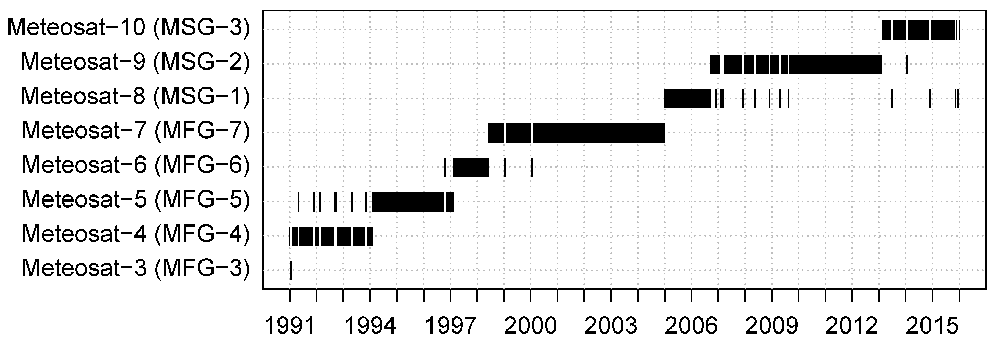
The COMET CFC CDR was produced by using the MVIRI sensor on Meteosat 3–7 and the Spinning Enhanced Visible and Infrared Imager (SEVIRI) sensor on Meteosat 8–10, as visualized in Figure 1. MVIRI is a radiometer that measures the Earth’s disk every 30 min in 3 spectral bands (the so-called Meteosat heritage channels) covering visible and infrared wavelengths: the broadband Visible channel (VIS, 500–900 nm), the Water-Vapor absorption channel (WV, 5.7–7.1 $\mathsf{\mu }$m), and the thermal Infrared channel (IR, 10.5–12.5 $\mathsf{\mu }$m). Only the VIS and IR channels were used since the WV band has limited power for cloud detection. SEVIRI scans the Earth’s surface every 15 min in 12 spectral channels ranging from the visible to the thermal infrared. For SEVIRI, we employed only the two visible channels (560–710 nm and 740–880 nm) to simulate MVIRI’s broadband VIS channel and the thermal infrared channel (9.8–11.8 $\mathsf{\mu }$m) to most closely “mimic” Meteosat heritage channels on MVIRI. The new International Satellite Cloud Climatology Project (ISCCP) H-series algorithm follows the same strategy of “downgrading” several satellite types and generations to a common set of two (one VIS and one IR) channels [26,27].

Equations and scientific background on every methodological aspect outlined hereafter can be found in the algorithm description [28]. A detailed performance assessment of COMET can be found in the validation report [29,30]. Both works are publicly available from CM SAF and have undergone an independent peer review process under the supervision of EUMETSAT. The COMET CFC CDR dataset is freely available from CM SAF [31]. The next six methodological subsections thus do not duplicate the existing technical report on how the algorithm works, but rather provide the scientific rationale for why the methods were chosen and how they differ from previous methods of satellite-based CFC estimation.

2.1. Calibration: Trust Your Space Agency

The GCOS stability requirements outlined in the Introduction can only be reached by starting from accurately-calibrated radiances, also known as the Fundamental Climate Data Record (FCDR). Our earlier Meteosat global radiation CDR [16] for instance shows breaks prior to 1994 despite relying on a self-calibration procedure using bright clouds as a stable target [32]. Trying to make up for sensor calibration issues within the retrieval of the physical variable cannot guarantee a stable CDR. First, calibration is best carried out on the primary variable rather than on a derived quantity. Second, apparently stable targets in either the solar or thermal domain may still be affected by seasonal variation and long-term trends in the climate system.

COMET employs re-calibration coefficients for the IR channel covering the whole Meteosat First Generation archive. They were developed by EUMETSAT by use of the High-resolution Infrared Radiation Sounder (HIRS) on board the NOAA polar platforms as reference measurements [33]. The method of re-calibration was built upon the GSICS methodology, mainly for collocating the Meteosat measurements with reference measurements. However, the method generates new calibration coefficients, which enables computing radiances from the raw Meteosat measurements (counts). The GSICS method computes a radiance correction to operational Meteosat radiances. 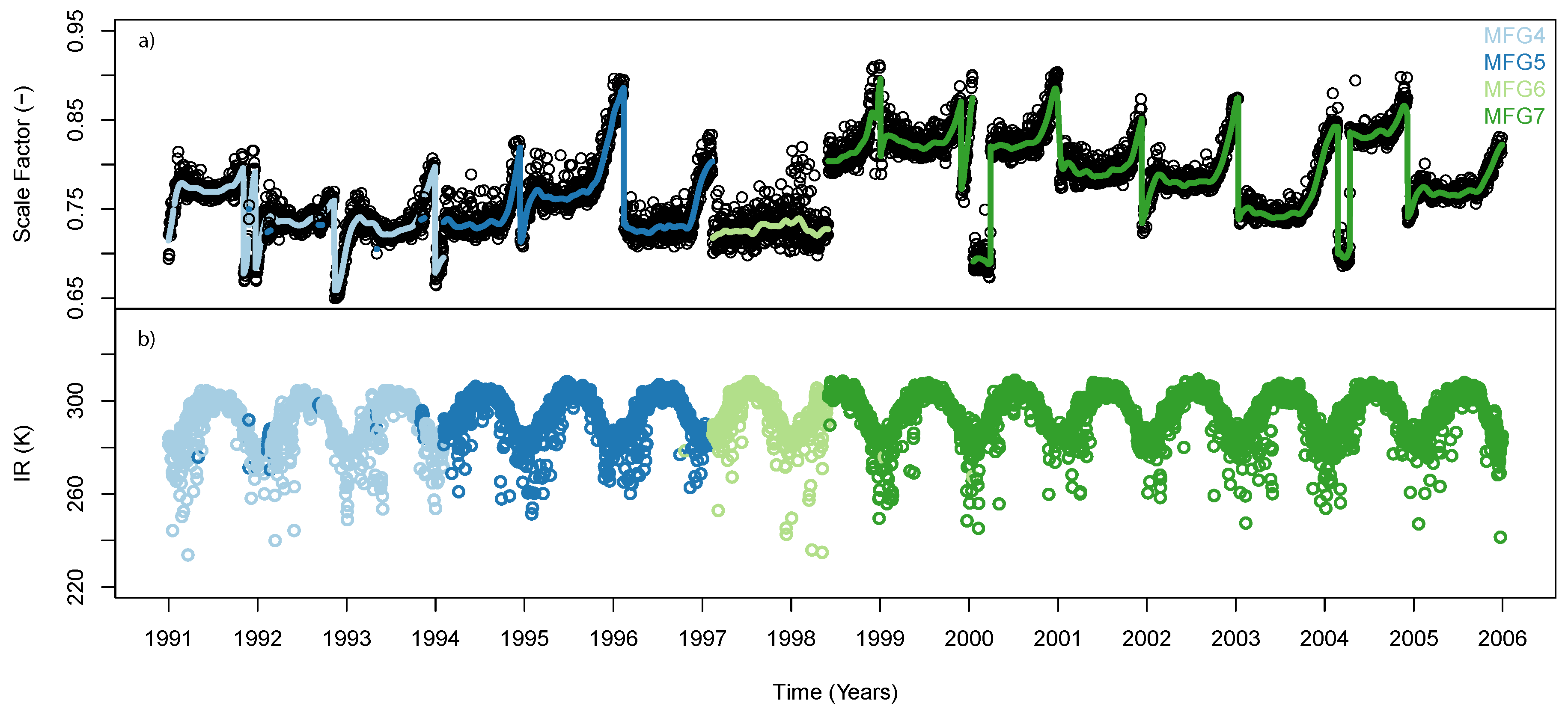Figure 2 visualizes the re-calibrated IR FCDR covering Meteosat-4–7 during 1991–2005. Only the historical MFG MVIRI period is shown for illustration since for MSG SEVIRI, the original calibration coefficients were used. The daily re-calibration coefficients (scale factor and offset) were smoothed with a 10-day Gaussian filter (Figure 2a; only the scale factor is shown). Diurnal variations in calibration were not accounted for since inter-calibration was performed against a polar-orbiting instrument and variations were not significant for spin-stabilized satellites. The result were stable brightness temperature time-series, as shown for the 15-year period over a desert pixel in Figure 2b. Compared to the original (non inter-calibrated) coefficients, the difference from MFG MVIRI to MSG SEVIRI was reduced from 1.83–0.28 K for the IR channel. The remaining difference was largely attributable to spectral and collocation differences between the two sensors [28] (Section 3). The long-term stability of the FCDR was further documented in [33]. The FCDR also guarantees a high decadal stability of <0.8 K/decade for the Meteosat-derived Land Surface Temperature (LST) CDR [34]. For the MVIRI solar channel, calibration factors were used as published by [35,36]. For MSG SEVIRI, the original VIS and IR calibration coefficients from EUMETSAT as part of their Level 1.5 files were used.

Our calibration strategy differed slightly from what was used by [26] for the new ISCCP H series, since they did not have new inter-calibration coefficients for geostationary sensors at hand. In ISCCP H radiances of geostationary sensors have been tied by the ISCCP team to radiances of polar sensors, while we could use a stable geostationary FCDR. We suggest that stable CDRs from historical sensors can best be achieved by separating FCDR and CDR production, but keeping those two tasks in close interaction. Knowledge on sensor gain changes, orbital maneuvers, spectral sensitivity, and the pre-processing of Level 0 satellite data are available at the respective space agencies and not necessarily with the CDR producer. This is analogous to the century-long surface measurements where quality screening and homogenization is most effectively done at the station operating the weather service [37]. We further practiced a cyclic exchange of calibration information, followed by CDR stability evaluation. Repeating the exercise 5–10 times between EUMETSAT and our team revealed technical difficulties with both the radiance and CDR production. It involved an efficient reality check where both parties gained knowledge, precision, and most importantly, confidence to publish their respective work.

2.2. Clear-Sky Reference: Solve the Chicken-and-Egg Problem

With only two channels available, cloud detection substantially benefits from a realistic quantification of the clear-sky signal as a reference. GEO satellite sensors measure with a high temporal frequency, which allows precisely following the diurnal course of each observed pixel. All-sky reflectances and brightness temperature have a large dynamic range between successive cloudy and clear-sky observations. Clear-sky reflectances and brightness temperatures on the other hand follow a predictable and continuous diurnal cycle. This is driven by surface anisotropy and surface energy balance. The high temporal resolution combined with a high predictability is used in COMET to separate clear-sky from cloudy observations. This is achieved by reconstructing the full diurnal cycle from clear-sky observations. Thus, instead of relying on external reference fields (such as albedo climatologies and modeled skin temperature), COMET retrieves a gap-free diurnal course of clear-sky reflectance and brightness temperature directly from the GEO observations. A model-based simultaneous inversion of cloud-screened clear-sky pixels was employed for this purpose.

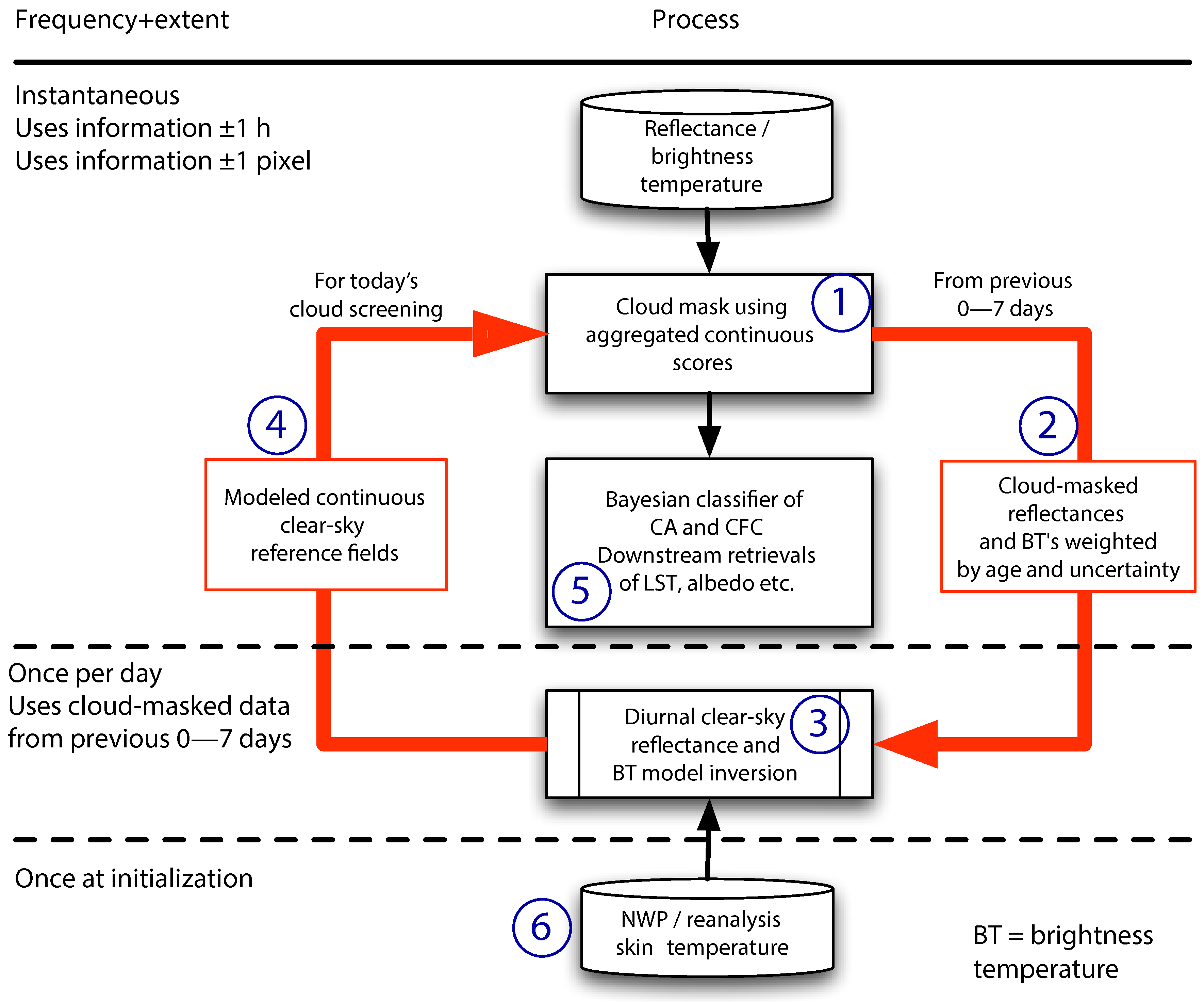
Figure 3 schematically visualizes this “implicit” clear-sky compositing. The following explanation starts from the top and continues in the clockwise direction. Blue numbers in the Figure correspond to the numbered items below.

• Calibrated reflectances and brightness temperatures were cloud-screened at every time step as in traditional cloud detection schemes. The cloud screening relied on a clear-sky reference for reflectance and brightness temperature for every time step. The cloud screening also employed spatial (±1 pixel) and temporal (±1 h) information.
• Each cloud screened (clear-sky) observation was weighted reciprocally by age and cloud detection uncertainty. The age was counted as number of days since the last cloud-free occurrence of a given satellite pixel. The detection uncertainty is a relative measure of potential cloud contamination in the clear-sky signal (see the next section for details). Clear-sky observations of a given satellite pixel were kept for a maximum of 7 days, and newer observations for a given time step replaced older ones. At the end of each day, this yielded an incomplete set (due to cloud cover) of clear-sky observations unevenly distributed over the diurnal cycle.
• Once per day, a gap-free clear-sky diurnal cycle was estimated by separately inverting a reflectance and a brightness temperature diurnal cycle model on the weighted clear-sky observations. These are semi-empirical models. They are governed by physical relationships such as the effect of satellite view and solar zenith angle on surface reflectance or the effect of solar and thermal heating on surface skin temperature. Compared to full surface energy and water balance schemes, they have a simpler representation of surface and atmospheric processes. They usually consist of one mathematical term and one parameter per process. For instance, clear-sky nocturnal decay of temperature is represented by an exponential term. The reflectance hot spot effect during noon is represented by a squared Sun-satellite backward scattering angle. Each model requires 3–7 parameters to be estimated per pixel and per day in order to fit a diurnal cycle to the observed data. More details on the diurnal cycle models can be found in [28] (Section 5), and diurnal cycle examples will be discussed further down (pink curves in Figure 5).
• The resulting modeled and gap-free diurnal cycle of reflectance and brightness temperature can be used as the clear-sky reference for subsequent (next day’s) cloud detection. In COMET, the cyclic procedure was applied in iterative mode using two passes of cloud screening. The clear-sky reference of the day before was used as a “first guess” to retrieve the current day’s clear-sky reference. This in turn served again as the “final” clear-sky reference for the current day’s cloud detection.
• For each cloud screened reflectance or brightness temperature, downstream algorithms can be run, such as a Bayesian CFC classifier or LST and surface albedo retrievals.

The careful reader may now object that there is no clear-sky reference and no cloud-screened clear-sky observations to fit a diurnal cycle model at the very beginning of the processing. However, the cloud detection requires that reference to be present as advocated above. Therefore, how can we get a clear-sky reference without having clear-sky observations in the first place? This chicken-and-egg problem is solved by injecting four NWP-based skin temperature values (for 0, 6, 12, and 18 UTC) at the very start of a processing and after very long periods (more than 7 days) of permanent cloud coverage (Number 6 in Figure 3). They were corrected for subgrid-scale elevation and augmented with the effect of water vapor and view zenith angle, so that they better corresponded to clear-sky ToA brightness temperature values. They constrained the diurnal cycle brightness temperature model on the first day and thus served as the initial clear-sky reference. This also means that with the absence of a clear-sky reflectance, the initial cloud screening used IR-only information. After 1–7 days of spin-up, enough clear-sky reflectance and brightness temperature observations were collected, and the cycle could run in a self-contained mode for reflectance and brightness temperature. For periods with >7 days of permanent cloud cover, NWP-based skin temperature was re-ingested during processing. Due to the high temporal sampling of Meteosat, this measure was only rarely necessary, making 7 days the maximum needed integration period. The integration period could be further reduced by looking forward and backward in time (and not just backward) for clear-sky pixels.

We found that the high temporal frequency provided by GEO sensors was sufficient to retrieve a clear-sky reference in the solar and thermal domain concurrently and use it for cloud detection without the need for external (possibly static) reference fields. A clear-sky reference derived from the satellite data itself is for instance also employed by the ISCCP H algorithm [26]. Compared to our approach of inverting diurnal cycle models of reflectance and brightness temperature, their compositing follows the commonly-used surface-type dependent threshold and pixel selection process. We found that a model-based inversion of the diurnal cycle of GEO reflectances and brightness temperatures was highly robust with respect to outliers (cloudy pixels in the clear-sky composite), as also demonstrated by [38]. While the latter focused on the joint retrieval of surface albedo and aerosol optical thickness, we applied it to cloud screening and CFC retrieval.

2.3. Error Propagation: Get Rid of Binary Decisions

The COMET cloud detection has been inspired by the MODIS [39] and the Separation of Pixels Using Aggregated Rating over Canada (SPARC) [8] cloud detection schemes. The continuous formulation of cloud detection confidence in these two schemes has a number of benefits over most historical binary cloud masks such as the NWC SAF [21], Clouds from AVHRR (CLAVR) [40], ISCCP [26,41], or the AVHRR Processing scheme Over cLouds, Land and Ocean (APOLLO) [42] using classification trees.

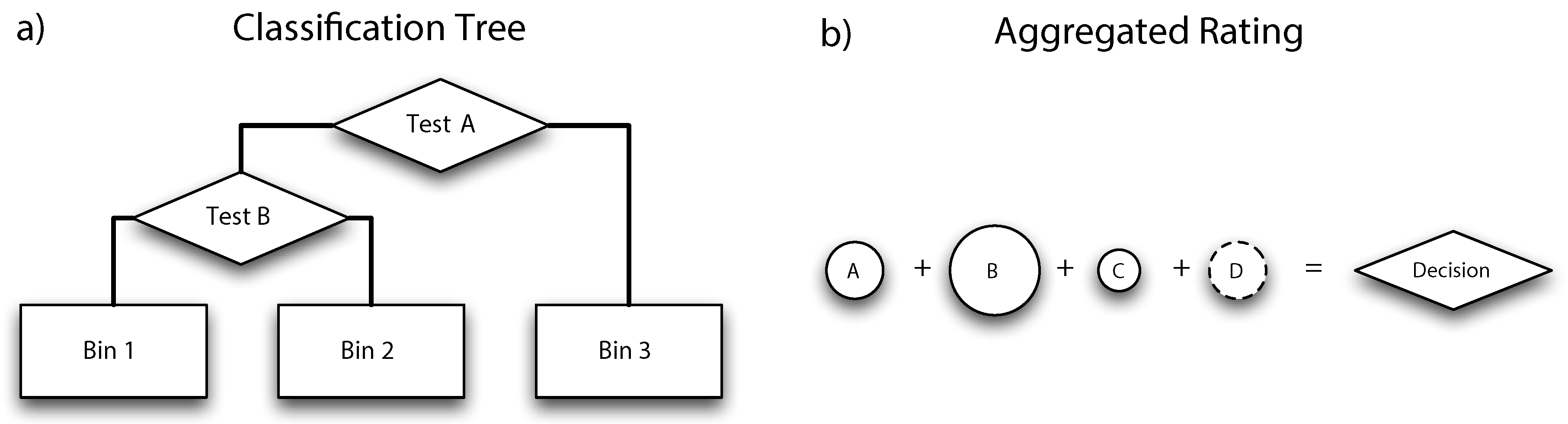
In a classification tree, every binary test depends on the successful execution of previous (upstream) tests. Misclassification can occur since upstream tests influence the effectiveness of downstream tests. As schematically drawn in Figure 4a, Test B depends on Test A. Test B is never actually considered if Test A results in Bin 3. There are often good reasons for not executing all tests for every scene condition (e.g., day vs. night illumination conditions, channel availability, very low brightness temperature, etc.). Such fine tuning requires expert judgment and a laborious manual training. Would not it be great if all tests could be considered in order to make a statistically-motivated decision? This is where the SPARC methodology of an aggregated rating with continuous scores comes into play (Figure 4b). A decision is only made once all scores have been calculated. Each score has a value range from negative (clear) to positive (cloudy), 0 being “undecided”. Each score can be weighted. Weights can be estimated with training data, or they can also depend on external drivers such as solar zenith angle. As exemplified here, score A may be a weak spatial variance test, and Score B with a higher weight may be a strong 10-$\mathsf{\mu }$m brightness temperature test. If Score A indicates clear and Score B cloudy, the result is a a fuzzy instead of a binary decision. The aggregated rating is the sum of all weighted scores and will likely lie between undecided and cloudy.

Common cloud masks yield a low number of cloud detection bins if not a binary classification. These are usually clear, cloud-contaminated, and cloudy (e.g., the NWC SAF scheme [21]). The cloud detection threshold for a cloud mask is set from clear-sky conservative (only fully clear-sky pixels) to cloud conservative (only fully cloudy pixels). The former is the most common and used for the retrieval of surface properties, while the latter is needed for the retrieval of cloud properties [43]. Classification trees with binary tests require fine tuning of binary decision thresholds for each test. Thresholds often depend on land use, time of day, or other orbital factors, as well as on calibration. Land use information is either static or not timely updated and consists of broad land use classes [44]. However, the Earth’s surface is subject to abrupt or continuous land use changes or seasonal phenological variability. Static land-use-dependent cloud cover thresholds may thus lead to false trends in cloud cover climatologies. The dependence of cloud detection from the underlying surface can be minimized by removing the clear-sky reference prior to running the test. Only the difference between the all-sky and the clear-sky signal is of relevance for cloud detection and not the absolute reflectance or brightness temperature.

COMET applies the aggregated rating of continuous scores to the two common channels of MFG MVIRI and MSG SEVIRI sensor data by using a fixed set of four scores (

Table 1. Continuous scores utilized for cloud detection and Bayesian CFC estimation.

No.	Score	Function
1	${\mathrm{T}}_{\mathrm{score}}$	Clear-sky minus all-sky brightness temperature score. This score is negative or close to 0 with no clouds present and becomes positive if clouds are colder than the underlying surface. It is useful to detect cold and high clouds during day and night.
2	${\mathrm{B}}_{\mathrm{score}}$	All-sky minus clear-sky reflectance score. This score is negative or close to 0 with no clouds present and raises if clouds are brighter than the underlying surface. It is useful to detect bright clouds during the day.
3	${\mathrm{STR}}_{\mathrm{score}}$	Spatio-temporal variability of all-sky reflectance. This score is close to 0 with no clouds present and raises if reflectance varies spatially within $\pm 1$ pixel and temporally within $\pm 1$ h. A spatial variability (e.g., from a land/sea border) or a temporal variability (e.g., from changing illumination) alone does not raise the score. It is useful to detect moving clouds or developing clouds on the sub-grid scale during the day.
4	${\mathrm{TV}}_{\mathrm{score}}$	Temporal variability of all-sky brightness temperature. This score is close to 0 with no clouds present and raises if brightness temperature varies temporally within $\pm 1$ h. It is useful to detect moving clouds or developing clouds on the sub-grid scale during the day and night. Additionally testing for variability in space like with the ${\mathrm{STR}}_{\mathrm{score}}$ did not yield any additional performance.

). Scores 1 and 2 are state scores, which strongly rely on the cyclic clear-sky reference estimation described in the previous section. Scores 3 and 4 exploit the spatial and temporal variability of all-sky reflectances and brightness temperatures. A detailed description of scores, their weights, and the aggregation equations can be found in [28] (Section 4). All four scores were used during daytime, while only the two IR scores 1 and 4 were used during nighttime. The scores did not depend on any land use information since the state scores were evaluated relative to the clear-sky signal and the variability scores had zero variability as a reference.

The aggregated rating method has two side benefits: it yields a flexible cloud detection threshold and a concurrent cloud detection uncertainty. Since the aggregated rating is a continuous measure, a user-defined cloud/clear threshold can be set posterior to the cloud detection. With a chosen cloud/clear threshold, also the uncertainty function can be defined either heuristically or by observational support. In our case, we heuristically defined a maximum uncertainty for the aggregated score of 0 (undecided cloud state) and decreased the uncertainty by use of a Gaussian distribution towards negative clear or positive cloudy ratings. A cloud detection uncertainty with observational support also realized in COMET with the Bayesian classifier is described further down. The resulting cloud detection uncertainties can be utilized to weight cloud-screened observations as input for the diurnal cycle inversion or for any downstream Essential Climate Variable (ECV) processing requiring cloud-free or cloudy observations.

COMET utilizes continuous scores relative to a clear-sky reference since this strategy firstly avoids land-use-dependent tuning and potential artifacts. Secondly, with continuous scores, the user is free to choose a binary cloud/clear threshold depending on the intended application. Setting the threshold posterior to the cloud detection spares a re-calculation of the cloud detection for each downstream application. As will be demonstrated for the CFC calculation, continuous scores are the prerequisite for the operation of a Bayesian classifier.

2.4. Single Imagery? Analyze the Full Diurnal Cycle

This section uses real examples to demonstrate the above-described theoretical concepts of clear-sky reference retrieval and cloud detection. We guide through the steps of inverting full diurnal cycles of clear-sky reflectance and brightness temperature for retrieving cloud-free and gap-free clear-sky reference fields. Combined with temporal information and continuous cloud scores, these reference fields enable a reasonable cloud detection with only two channels.

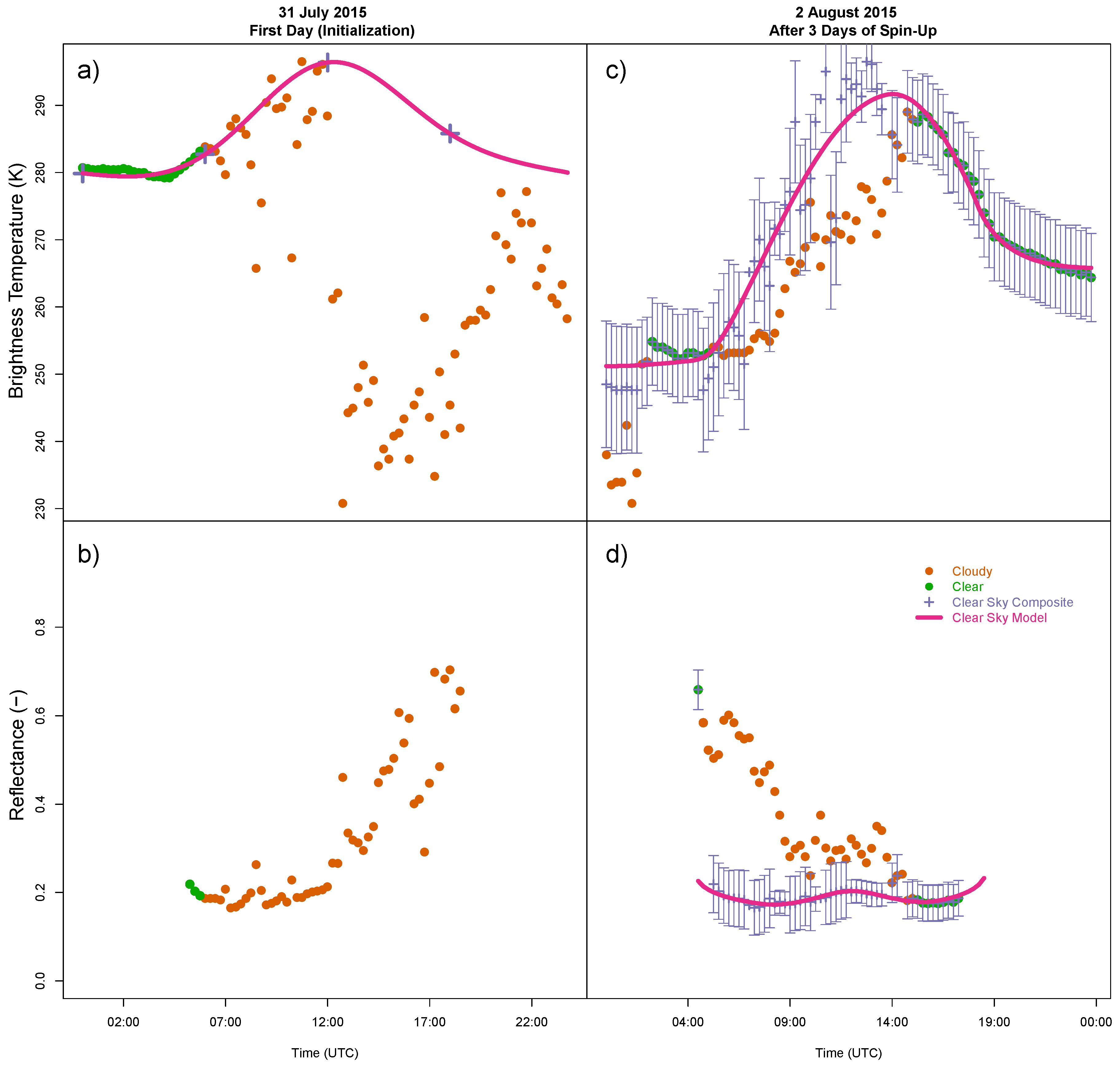
Figure 5 shows brightness temperature and reflectance time-series for two days over the temperate site Payerne (WMO synoptic observation site #06610). This example processing was started on 31 July 2015 with no a priori information on clear-sky brightness temperature and reflectance. On the first day, four NWP-based skin temperature values at 0, 6, 12, and 18 UTC (Figure 5a, large blue crosses) served as a surrogate for (yet) unavailable clear-sky brightness temperature observations. They constrained a first parameterized diurnal cycle of brightness temperature (Figure 5a, pink curve). This gap-free diurnal cycle of brightness temperature was then used as a reference by the cloud detection. It allows separating the all-sky brightness temperature (Figure 5a, filled circles) and reflectance (Figure 5b, filled circles) into clear (filled green circles) and cloudy (filled orange circles).

Figure 5. Estimation of the clear-sky reflectance and brightness temperature diurnal cycle by use of parametric models. On the first day of processing, four NWP-based skin temperature predictions (a, large blue crosses) were used to estimate a continuous diurnal cycle of brightness temperature (a, pink curve). This is the reference for the first clear/cloudy separation (clear = filled green circles; cloudy = filled orange circles). Clear-sky reflectance is not yet available on the first day (b). After 3 days, enough clear-sky observations (blue crosses and error bars) of brightness temperature (c) and reflectance (d) had been collected. This allows a high quality parametric estimation of both clear-sky brightness temperature and reflectance diurnal cycles (pink curves), which are the foundation for subsequent cloud detections.

Figure 5. Estimation of the clear-sky reflectance and brightness temperature diurnal cycle by use of parametric models. On the first day of processing, four NWP-based skin temperature predictions (a, large blue crosses) were used to estimate a continuous diurnal cycle of brightness temperature (a, pink curve). This is the reference for the first clear/cloudy separation (clear = filled green circles; cloudy = filled orange circles). Clear-sky reflectance is not yet available on the first day (b). After 3 days, enough clear-sky observations (blue crosses and error bars) of brightness temperature (c) and reflectance (d) had been collected. This allows a high quality parametric estimation of both clear-sky brightness temperature and reflectance diurnal cycles (pink curves), which are the foundation for subsequent cloud detections.

In Figure 5a, brightness temperature values until 6 UTC follow or exceed the clear-sky reference. They were detected as clear. Brightness temperature values from 6–12 UTC also followed the clear-sky reference. They were set to cloudy due to their substantial temporal variability relative to the clear-sky reference. This was likely caused by moving thin or low clouds. A few all-sky reflectances just after sunrise in Figure 5b corresponding to cloud-free brightness temperatures in Figure 5a are marked as clear as well. During spin-up, only thermal information was used for cloud detection since the clear-sky reference was (yet) missing.

On 2 August 2015, after 3 days of spin-up, a history of clear-sky brightness temperatures and reflectances (Figure 5c,d, blue circles including uncertainty bars) has been built. The uncertainty reflects both the clear-sky pixel’s age and the uncertainty of the underlying cloud detection. This uncertainty, although relative and not absolute, was key for the success of the clear-sky inversion. In Figure 5c, too low brightness temperature composites between 0 and 2 UTC, around 6 UTC, and 12 UTC did not have an impact on the modeled diurnal cycle. They had a higher uncertainty, which was either due to their age (too long since the last clear-sky observation) or quality (uncertain clear-sky state, possibly cloud contaminated).

The modeled clear-sky reference was superior to the one that would be simply composited from instantaneous cloud-screened values. It was based on the same information, but was augmented with semi-empirical relationships (the model), which related individual values in time. This is demonstrated in Figure 5d with a single high reflectance composite value of around 0.65 (filled green circle, with a blue cross inside and error bars) at around 4 UTC, which was input into the clear-sky inversion (pink curve). The resulting clear-sky model ignored this value due to around 40 other input values that much better corresponded to the semi-empirical clear-sky model. The diurnal cycle model inversion yielded clear-sky estimates that were more robust than the individual contributing clear-sky observations. The inversion can make up for instantaneous cloud screening errors.

We have seen in Figure 5a that exploring the temporal variability enabled classification of thin moving clouds. We also see in Figure 5c between 6 and 12 UTC that temperature signatures of <5 K can be detected as cloudy if they are put in relation to a realistic clear-sky reference. Without a clear-sky reference inheriting the information from a full day and without using information on temporal (and spatial) variability, such a small brightness temperature signature would go undetected. It would be classified as clear-sky when using only information of two broadband channels on the instantaneous (image-by-image) level.

2.5. Bayesian Classifier: Exploit State and Variability

The cloud detection described above used the aggregated rating to separate clear-sky from cloudy pixels in order to feed purely clear-sky pixels to the cyclic clear-sky inversion. Such a satellite-based clear-sky conservative cloud detection is not comparable to ground-based climatological CFC observations. Our intent was to reproduce CFC of ground-based synoptic observations (SYNOP), so that COMET CFC could be compared to time-series extending into the pre-satellite era. SYNOP CFC is non-linearly related to a satellite-based cloud estimate. In the latter, “radiative fluxes” are analyzed in spectral domains that exceed the human eye’s spectral response. Instead of explicitly transferring this rule set to satellite observations, COMET CFC was calculated by use of a Bayesian classifier constrained by SYNOP CFC. Conditional occurrence probabilities were derived by the CFC class with >$3\times {10}^6$ CFC observations from 339 quality-screened and homogeneity-tested SYNOP sites [28]. According to the observational guide of the World Meteorological Organization [45], a single cloud in the sky modifies the 0 to a 1 Okta class, respectively the 8 to a 7 Okta class for a single gap in cloud cover. We have tried to classify the 0 and 8 Okta classes separately. We failed to find any differentiation from the 1 and 7 Okta classes with the available spectral, temporal, and spatial information. Therefore, following [46], the 0 and 1 Okta classes and the 7 and 8 Okta were joined to yield 7 CFC classes (1–7 Okta where 1 and 7 Okta are completely clear and completely cloudy).

The Bayesian classifier employs the same continuous scores as the above described cloud detection (Table 1). The often applied naive Bayesian classifier [13,47,48] however assumes scores to be independent (uncorrelated). It thus unconditionally multiplies their conditional probabilities. This simplification is tempting since it only requires one-dimensional histograms of conditional occurrence probabilities using 30–50 bins per histogram (see, e.g., Figure 3 in [13]). It is suitable for a sparse set of training observations. A full Bayesian classifier on the other hand would require N-dimensional histograms (N being the number of predictive scores), which can become under-constrained with even a high number of training observations.

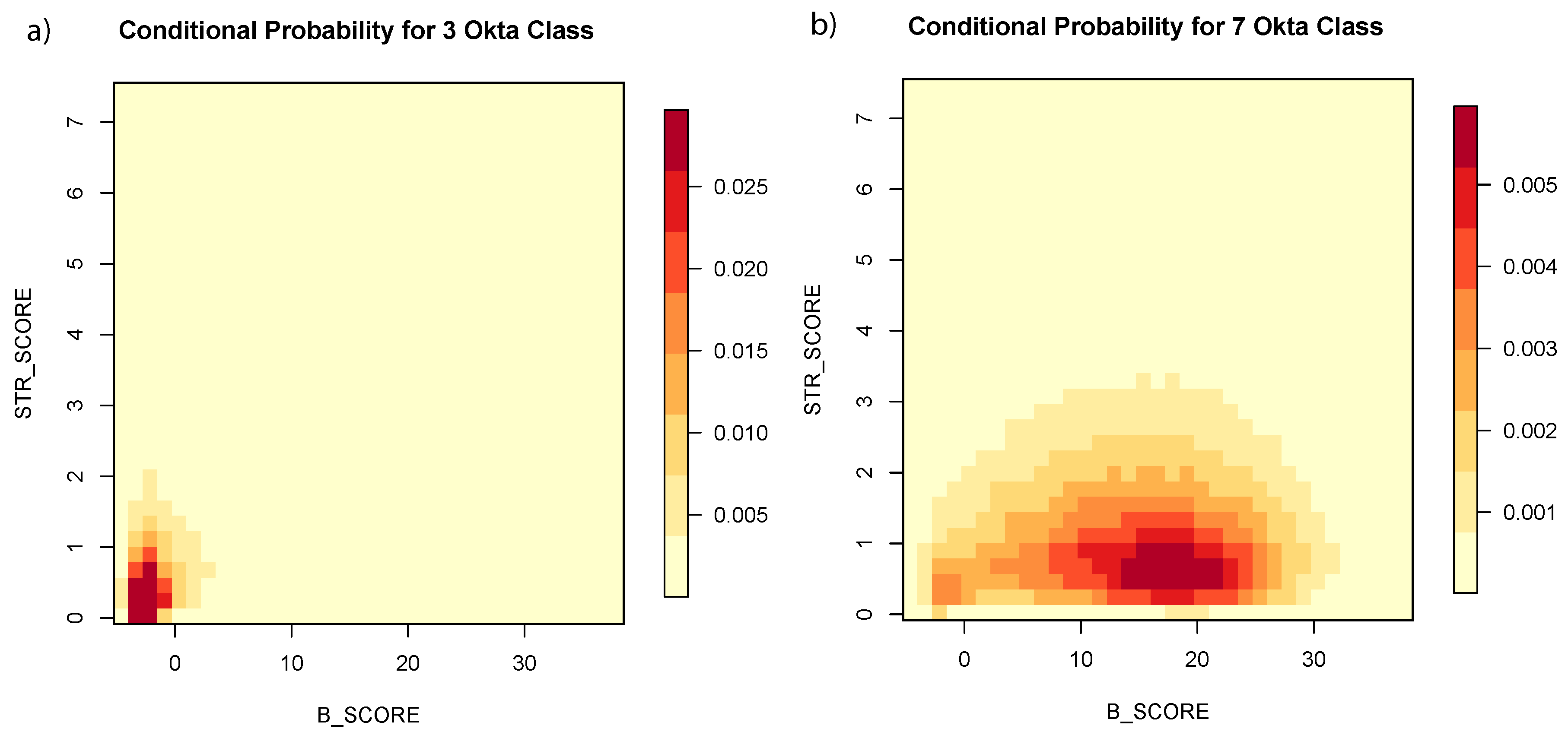
The Bayesian classifier implemented here explicitly exploited the best of both worlds by utilizing the co-variability of two scores at a time. Figure 6 exemplifies two-dimensional joint histograms for the solar channel. The dependence was always exercised between a state and a variability score (${\mathrm{B}}_{\mathrm{score}}$ vs. ${\mathrm{STR}}_{\mathrm{score}}$ and ${\mathrm{T}}_{\mathrm{score}}$ vs. ${\mathrm{TV}}_{\mathrm{score}}$). The probabilities shown are conditional to the absolute occurrence of the respective Okta class (and the plots thereof have different scale ranges). The 3 Okta class for instance occurred with a high conditional probability (red colors) when brightness (${\mathrm{B}}_{\mathrm{score}}$; all-sky minus clear-sky reflectance) was low. Concurrently, some spatio-temporal variability can be present (${\mathrm{STR}}_{\mathrm{score}}$ between 0 and 1). The 7 Okta class on the other hand occurred with a high conditional probability when the brightness was intermediate to high in combination with intermediate spatio-temporal variability. At the same brightness, but with higher variability, the same brightness yielded a lower probability for the 7 Okta class (and a higher probability for the 5 or 6 Okta class; not shown in Figure 6). With a naive Bayesian classifier, both axes in Figure 6 would be explored separately. However, it becomes clear with this example that they were related for cloud detection.

Co-variance information on state and variability was available in the data and it was harvested in COMET for accurate CFC estimation. With only two spectral channels available for cloud detection, the maximum use of all available information becomes even more essential. The spatio-temporal variance of VIS and IR was already successfully explored by a number of cloud classification schemes, such as the ISCCP H [26,27]. Our finding demonstrates that there can be a gain in precision if spatio-temporal variability is jointly analyzed with spectral state, for instance with a multi-dimensional or (optimally) full Bayesian classifier.

2.6. Agility: Develop on Time-Series

The computational demand of modern satellite-based CDR processing is substantial. Physical radiative-transfer-model-based retrievals or the cyclic clear-sky model inversions described above further increase processing time by orders of magnitude compared to traditional algorithms operating on an image-by-image sequence. With such requirements, CDR producers can often only exercise their algorithms on a few short “golden” periods during development. Temporal inconsistencies such as multi-year calibration drifts are revealed after month-long number crunching and analysis of the full CDR. Project time limitations further limit the number of full processing tasks prior to a release of the data to the users. Here, we choose a different strategy: agile algorithm development on time-series.

For COMET, the first step was to extract 25+ years of radiance time-series from the full domain image-based input dataset for 339 training and 237 homogeneous and gap-free validation sites. Already, this step has the power to reveal inconsistencies in the input radiances. They can be repeatedly exchanged with the respective space agency prior to CDR generation as described above. The analysis of long time-series is often more enlightening than the inspection of single images. The second step was to develop the actual algorithm. It involved inventing the cyclic clear-sky estimation, finding suitable CFC predictors, and calculating Bayesian conditional joint histograms for the 339 training sites. It also yielded the final parameter (in our case CFC) at the 237 validation sites for the full length of the envisioned CDR. The final step was then to run the algorithm over the full domain and for the full length to produce the CDR.

Our key message is that the second step is computationally very inexpensive. Running the algorithm over 25+ years for all 576 sites can be performed in less than one hour on high performance computer systems. This allows continuously re-evaluating the climatological stability of the algorithm across all possible land-based climate zones within the domain. Spatial inconsistencies such as coastal zone artifacts still need to be evaluated with a regional analysis over shorter periods. Algorithm changes are often motivated by case-driven detective work and not through analysis of the full CDR. For instance, low stratus may be undetected in winter over continental Europe. Fixing this systematic failure for a specific location (and possibly time of year) is needed in the first place. Re-checking the sensitivity of the full CDR to applied changes in the algorithm is then fundamental in order to accept a potential performance improvement.

Imagine having your final validation carried out several times a day, each time you make a change in the code? Validation can indeed be done prior to processing the CDR: there is simply no need to process the remaining 99.9% of the domain for this purpose. Compared to classical full-domain or granule-based development, we suggest an agile development on time-series where the algorithm can be exercised several hundred times on all validation sites prior to spending months of CPU time on the final CDR processing.

3. Results

All results and reference SYNOP datasets shown here were described in depth within the dataset validation report [29] and were discussed in [30]. COMET bias (trueness) was measured by the Mean Bias Error (MBE) metric, and precision was measured by the bcRMSE metric. Averaged over the 237 validation sites, the MBE of COMET CFC was −0.28% with a bcRMSE of 30% in absolute CFC units (0–100%) on the instantaneous collocations (

Table 2. Performance statistics of ClOud Fractional Cover dataset from METeosat First and Second Generation (COMET) CFC (%) compared with SYNOP at 237 sites based on instantaneous collocations. Number of collocations (N), mean COMET CFC ($\overline{\mathrm{COMET}}$), mean SYNOP CFC ($\overline{\mathrm{SYNOP}}$), Mean Bias Error (MBE) and bias-corrected RMSE (bcRMSE).

	N	$\overline{\mathbf{COMET}}$	$\overline{\mathbf{SYNOP}}$	MBE	bcRMSE
overall	20,931,127	55.47	55.75	−0.28	29.48
day	10,282,717	54.77	57.51	−2.74	24.43
night	7,800,066	55.67	52.53	3.14	34.47
DJF	5,138,479	62.63	65.34	−2.71	32.97
JJA	5,393,815	45.77	44.90	0.87	26.52
MFG	10,456,118	55.94	56.06	−0.12	30.13
MSG	10,475,009	55.00	55.44	−0.44	28.81

) and 7% for monthly means (not shown in Table 2). COMET CFC overestimated SYNOP (MBE = 3%) and was less precise during nighttime (bcRMSE = 34%) compared to daytime (bcRMSE = 24%). It underestimated SYNOP during Northern Hemisphere winter (MBE = −2.7%) compared to summer (MBE = 0.8%). Bias and precision between Meteosat First and Second Generation were almost identical despite comparing different time periods (1991–2004 for MFG to 2005–2015 for MSG).

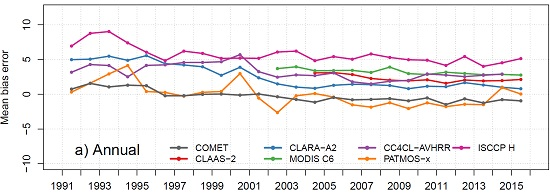
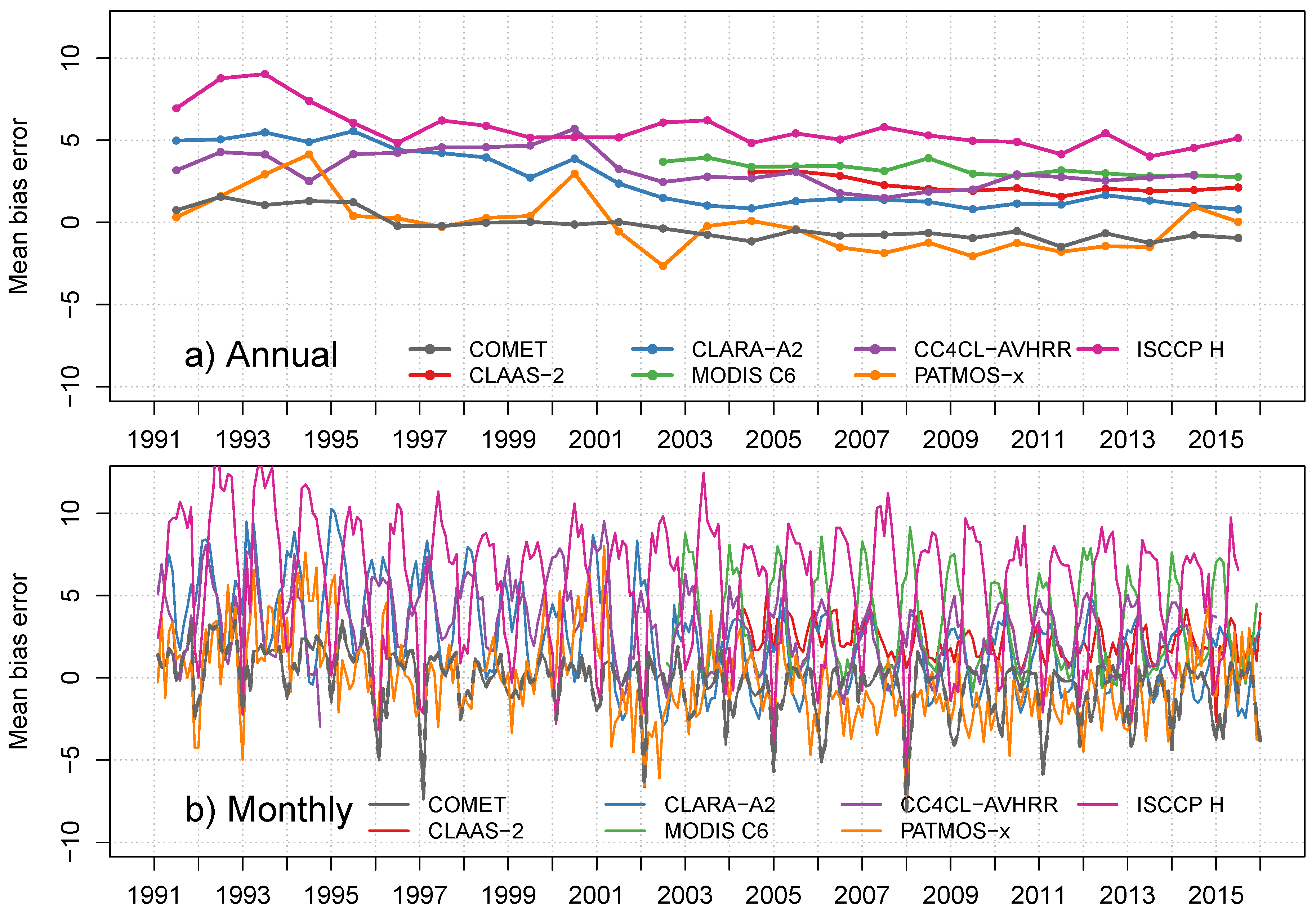
Figure 7 is reproduced from [29], but adds the new International Satellite Cloud Climatology Project (ISCCP) H [26,27] dataset (monthly mean cloud amount at one degree of spatial resolution) for inter-comparison. It displays the temporal evolution of yearly (a) and monthly (b) MBE averaged over the 237 SYNOP validation sites. The trend in bias of COMET was −0.94% per decade. This value lies between the GCOS-defined stability requirements for thick and thin clouds. This negative trend is related to the overestimation of CFC before 1996 and to a statistically-detectable break in 1996 (standard normal homogeneity test $T\left(k\right)>10.02$ for a 95% confidence level [30,49]).

When comparing to three long CDRs from polar-orbiting AVHRR sensors, COMET was most similar to PATMOS-x [50]. CC4CL-AVHRR [51] from the ESA Cloud CCI project and CLARA-A2 [52] from the EUMETSAT CM SAF yielded a more negative trend of bias and a 2–5% CFC overestimation. This negative trend likely comes from orbital drift with shifting overpass times. This incomplete diurnal sampling can influence CFC statistics [53,54], in particular at locations where cloudiness has a distinct diurnal cycle [55]. PATMOS-x would be subject to the same issues. In comparison to CC4CL-AVHRR-PM and CLARA-A2, instantaneous collocations with SYNOP data were used for PATMOS-x since it was not available as monthly means. This is evidence for the importance of either fully-resolving the diurnal cycle for CFC CDRs or for the need to compare strictly at collocated observation times [56].

CFC was overestimated by 3–5% in CLAAS-2 [57], ISCCP H [26], and MODIS [39]. They were derived by spatial aggregation of a possibly clear-sky conservative binary cloud mask, which can introduce biases depending on cloud regime (see above). It should be noted that the inter-comparisons presented here differed from global statistics for inter-compared datasets. Our analysis only covered the Meteosat field of view of COMET with high quality homogeneous SYNOP sites predominantly distributed in Europe and over land.

On the monthly scale, all datasets displayed a seasonal variation of MBE between 2 and 10%. Least seasonal variation was found for COMET, PATMOS-x, and CLAAS-2 and the highest for MODIS C6 and ISCCP H. The phase of seasonal variation also differed between datasets. COMET, ISCCP H, and to a lesser extent, PATMOS-x had a lower (or negative) MBE during Northern Hemisphere winter. MBE for CLARA-A2, MODIS, and CC4CL-AVHRR MBE on the other hand rose during winter. This points to a difference in how algorithms dealt with bright snow surfaces or low stratus coverage during Northern Hemisphere winter in Europe.

4. Discussion

With a cloud detection that implicitly calculates clear-sky reference fields, there is the risk of positive feedback. Cloudy pixels erroneously masked as clear-sky would raise clear-sky reflectance and lower clear-sky brightness temperature of reference fields. Such cloud-contaminated reference fields would in turn yield even more cloudy pixels marked as clear-sky. After a few days of application, the clear-sky reference fields would be fully cloud contaminated. Why is this “cat bites it’s own tail” issue not an issue here? We first set the cloud detection threshold to clear-sky conservative. Second, the diurnal cycle model inversion using weighted clear-sky observations was robust to missed clouds as demonstrated above. These measures turned the whole cycle into a stable loop. The other potentially problematic case is a rapid change in surface properties such as snowfall in autumn. Without a proper spectral snow/cloud separation, this change can generate a few days of exaggerated cloudiness (during daytime only) until a new clear-sky visible reference has been built up. A similar situation can occur for clear-sky brightness temperature driven by synoptic changes of surface skin temperature. A temperature drop of, e.g., 5 K, from one day to the next could generate a false cloud signal until the daily clear-sky inversion has caught up with the changed ambient conditions. This problem was mitigated by running the cloud detection twice, as described above. A first guess cloud detection with the last day’s clear-sky inversion provided new clear-sky brightness temperatures for estimating the current day’s clear-sky diurnal cycle for a final CFC estimate. Potentially false cloud signals were also minimized by the two variability scores, which were insensitive to constant shifts between the all-sky and the clear-sky signal.

The first version of the retrieval had some issues. During Northern Hemisphere winter, COMET underestimated CFC by 1–5%. CDRs from polar-orbiting satellites showed exactly the opposite (Figure 7b). We hypothesized that the misclassification of cloud-free snow into clouds or higher Sun zenith angles might be responsible for this result. The underestimation of COMET can be explained with the use of state scores that are based on the difference between the all-sky signal to a clear-sky reference. For low stratus, there was simply no more cloud signal in the broadband solar or thermal spectrum after subtracting the clear-sky reflectance or brightness temperature of cold winter land surfaces. The all-sky and the clear-sky signals of snow and low stratus were almost identical. If all-sky matched clear-sky, the scene was identified as clear-sky. This was also the case when too many cloudy observations propagated into the clear-sky compositing and thus apparently could violate the above-described stable loop. We have found that it did not harm the clear-sky diurnal cycle compositing due to the following reason. Consider a winter inversion of the low stratus cloud (e.g., with reflectance 0.6 and brightness temperature 276 K). It has almost the same signature as the underlying surface (e.g., with reflectance 0.55 and brightness temperature 273 K). With the available spectral capabilities, cloud and clear-sky look the same. Therefore, the cloudy signal for this low stratus can be safely considered as realistic input to the clear-sky inversion. The missed cloud will however yield a too low CFC estimate as discussed before. We have also examined whether seasonal biases of SYNOP CFC could be responsible for the underestimation of cloudiness during winter. Checks with ceilometer-based CFC observations at individual sites in Switzerland revealed only the known day-night bias (of around 0.5 Okta), but not a seasonal bias. This justifies efforts to improve Northern Hemisphere winter cloud detection with our two-channel scheme.

The inhomogeneity in the time-series before and after 1996 could be related to remaining calibration issues, but it is not concurrent to any satellite change. COMET also showed a decrease in accuracy at view zenith angles beyond 55${}^{\circ }$. Next, by using a fixed time window of 0–24 UTC for the clear-sky diurnal cycle inversion, the CFC estimate can have “visually unappealing jumps” between two days. Finally, despite being unbiased to MSG as shown above, MFG displays a 10% higher diurnal CFC range than MSG. This might be related to small differences in spectral response (the radiances have not been translated to a common spectral response in this version), the channel’s dynamic range, or simply due to differences with temporal acquisition frequency (15 versus 30-min steps).

Some of these issues, like the small inhomogeneity in 1996, shall be possible to correct. For others, like the low stratus underestimation in Northern Hemisphere winter over continental Europe, two channels may simply not contain enough information. However, low stratus has a thermal signature that differs from the clear-sky land surface: it has no diurnal cycle. The non-existing temporal variability in relation to the diurnal temperature range of the clear-sky reference could be explored on the 12–24-h scale.

The algorithm requires a spin-up of several days, which is more similar to prognostic NWP and climate models than to satellite retrieval schemes. It also requires the concurrent analysis of a full day’s set of reflectances and brightness temperatures, which is fine for climate applications. In order to be useful in now-casting applications, the last day’s clear-sky inversion could be applied. The clear-sky inversions are computationally more demanding than empirical image-by-image cloud detection schemes. Depending on the length of the chosen spin-up period, CFC can slightly differ for a given date and location. However, this novel concept COMET meets GCOS bias, precision, and stability requirements for multi-decadal CFC CDRs bridging two generations of GEO sensors.

We have been asked whether the simultaneous retrieval of clear-sky reference fields or the agile development on radiance time-series would be applicable to polar sensors. The diurnal inversion of brightness temperature requires 4–8 daily clear-sky observations to estimate three parameters. As shown, it can be augmented with an NWP-based a priori reference. This requirement is met by the joint polar system operated by the U.S. and European space agencies, but may be violated for early AVHRR periods. It may be more successful for higher latitudes with several daily overpasses per sensor if the clear-sky diurnal cycle of snow-covered surfaces can be modeled well enough. Similarly, agile development on time-series might be more useful for high latitude areas with a higher frequency of observations, but should be applicable to polar sensors as well. Furthermore, development on time-series might not be an option for CDRs with no site-based validation data (e.g., buoys, aircraft-based, or satellite-based reference data).

The high number of Synoptic cloud observations (SYNOP) available for the whole Meteosat period and covering the Meteosat Field of View (FoV) was our choice for the absolute reference. SYNOP CFC has been measured since the late 19th Century, making it an ideal candidate for climate analysis. It however is at stake at national weather services due to the shortage of human observers. Replacing SYNOP CFC with satellite-based CFC is not trivial due to the complex manual decision process when observers quantify clouds [58]. Many current cloud retrieval schemes are thus trained with the space-based reference from Cloud-Aerosol Lidar and Infrared Pathfinder Satellite Observation (CALIPSO) / Cloud-Aerosol Lidar with Orthogonal Polarization (CALIOP) instead SYNOP [13,52]. CALIPSO/CALIOP is a reference for both PATMOS-x and CLARA-A2, and our validation has also extensively used it [30]. Due to its limited time extent, we experienced that CALIPSO/CALIOP is highly suitable for algorithm development especially over oceanic areas where SYNOP is missing. CALIPSO/CALIOP is difficult to use as a reference for testing the precision and stability of CDRs due to its limited time extent. It also requires defining a cloud/clear threshold with dependence on the minimum detectable Cloud Optical Depth (COD), as demonstrated by [59]. CALIPSO/CALIOP is providing a COD that is independent of the underlying surface type and illumination condition. It can thus be used to train physically-based COD retrievals. On the other hand, SYNOP data are non-linearly related to COD and include spatial information not available with CALIPSO/CALIOP. We also found that SYNOP CFC was subject to a day-night bias of around 0.5 Okta due to clouds observable at farther distances during day than during night [58]. SYNOP is not available over many “difficult” oceanic areas such as the low stratocumulus area west of Africa where current satellite-based cloud CDRs differ. The uneven spatial distribution of SYNOP sites could be mitigated by the use of SYNOP-like CALIPSO data over ocean trained with SYNOP CFC over land. However, considering the flaws of SYNOP CFC, a suitable absolute reference for satellite-based CFC retrieval has yet to be found. The question needs to be asked about how adequate SYNOP CFC is for climate monitoring and change detection. Might a “radiation-based” view on clouds be more useful than a location- and observer-dependent CFC estimate? Do we need to find a transfer function from SYNOP CFC to satellite-based cloud properties instead of the other way round?

5. Conclusions and Outlook

The main strategy of COMET is not to waste any information contained in historical sensor data. COMET replaces missing spectral information by carefully exploiting the full temporal and spatial resolution of GEO sensors. The implicit clear-sky estimation together with the joint use of state and variance information for pixel-wise CFC estimation comprises the most important and innovative pieces of the COMET CFC algorithm. Well-calibrated radiances are the foundation for such an achievement.

The algorithm now consists of a clear-sky conservative cloud detection using aggregated rating to build the clear-sky reference fields, which in turn are used to build continuous scores for both cloud detection and continuous CFC estimation. The two cloud schemes could be replaced by a single CFC estimation: a clear-sky conservative CFC threshold (e.g., CFC = 0–10%) could be used to determine clear-sky pixels as input to the cyclic clear-sky inversion. Furthermore, the Bayesian CFC estimator is now built on separate two-dimensional VIS and IR histograms. This is an efficient and effective compromise between the naive and a full-dimensional Bayesian classifier. We still suggest to explore more dimensions or to consider more driving features such as the clear-sky reflectance and brightness temperature. Instead of explicitly resolving additional dimensions, a vectorized approach for multivariate feature fields might be an option [60].

We have successfully applied COMET for downstream LST retrieval [61]. The homogeneity and temporal stability of COMET and phase and amplitude of COMET diurnal cycles have been proven to be realistic [62]. As a next step, we are going to extend the algorithm framework behind COMET called “GeoSatClim” for a joint retrieval of all four Surface Radiation Balance (SRB) components. We will also include the early Meteosat sensors from the 1980s. Within the WMO SCOPE-CM project SCM-03 [63], COMET CFC is extended to the GEO sensors of the National Oceanic and Atmospheric Administration (NOAA) and the Japan Meteorological Agency (JMA). This will allow retrieving surface albedo fully exploiting the geostationary “ring” of GEO satellites.

With this overview, we would like to motivate CDR developers to invent and evaluate new methods to retrieve multi-decadal CDRs bridging several sensor generations. While acknowledging that cloud physical parameters like cloud droplet size cannot be estimated with two broadband channels, historical satellite sensor archives still contain exploitable and useful climate information. The path shown here with a common set of reference channels is only one possibility to achieve decadal stability. Geospatial models and multi-observational constraints in satellite climatology have yet to be explored. Possible examples are the treatment of varying station density in spatial reconstruction (e.g., by use of reduced space optimal estimation [64]) or the non-contemporaneous combination of station and satellite data (e.g., for sunshine gridding [65]). The same applies to optimal estimation by all-sky radiative transfer model inversion across sensor generations, where a higher spectral and temporal density of modern sensors can be harvested in favor of decreasing uncertainty with unchanged overall bias.