Classifying Inundation in a Tropical Wetlands Complex with GNSS-R


1
Planetary Radar Radio Science Systems Group, Jet Propulsion Laboratory, California Institute of Technology, Pasadena, CA 91109, USA
2
Carbon Cycle and Ecosystems Group, Jet Propulsion Laboratory, California Institute of Technology, Pasadena, CA 91109, USA
3
Department of Earth and Atmospheric Science, The City College of New York, City University of New York, New York, NY 10031, USA
4
Earth and Environmental Sciences Program, The Graduate Center, City University of New York, New York, NY 10016, USA
*
Author to whom correspondence should be addressed.
Remote Sens. 2019, 11(9), 1053; https://0-doi-org.brum.beds.ac.uk/10.3390/rs11091053
Submission received: 10 April 2019
/
Revised: 30 April 2019
/
Accepted: 2 May 2019
/
Published: 4 May 2019
Abstract
:The use of global navigation satellite system reflectometry (GNSS-R) measurements for classification of inundated wetlands is presented. With the launch of NASA’s Cyclone Global Navigation Satellite System (CYGNSS) mission, space-borne GNSS-R measurements have become available over ocean and land. CYGNSS covers latitudes between ±38°, providing measurements over tropical ecosystems and benefiting new studies of wetland inundation dynamics. The GNSS-R signal over inundated wetlands is driven mainly by coherent scattering associated with the presence of surface water, producing strong forward scattering and a distinctive bistatic scattering signature. This paper presents a methodology used to classify inundation in tropical wetlands using observables derived from GNSS-R measurements and ancillary data. The methodology employs a multiple decision tree randomized (MDTR) algorithm for classification and wetland inundation maps derived from the phased-array L-band synthetic aperture radar (PALSAR-2) as reference for training and validation. The development of an innovative GNSS-R wetland classification methodology is aimed to advance mapping of global wetland distribution and dynamics, which is critical for improved estimates of natural methane production. The results obtained in this manuscript demonstrate the ability of GNSS-R signals to detect inundation under dense vegetation over the Pacaya-Samiria Natural Reserve, a tropical wetland complex located in the Peruvian Amazon. Classification results report an accuracy of 69% for regions of inundated vegetation, 87% for open water regions, and 99% for non-inundated areas. Misclassification of inundated vegetation, primarily as non-inundated area, is likely related to the combination of two factors: partial inundation within the GNSS-R scattering area, and signal attenuation from dense overstory vegetation, resulting in a low signal.
1. Introduction
Wetlands cover a small portion (less than 5%) of Earth’s ice-free land surface [1], yet they have major impacts on global biogeochemistry, hydrology, and biological diversity. They are the largest natural source of atmospheric methane, with their extent and inundation variability playing a large role in ecosystem dynamics, contributing roughly 20–40% of global methane emissions [2]. However, methane emissions from wetlands remain one of the principal sources of uncertainty in the global atmospheric methane budget, primarily because the distribution and evolution of atmospheric CH4 sources and sinks are poorly resolved [3].
Climate and anthropogenic-driven changes to wetlands can potentially create significant feedbacks to atmospheric methane through effects on methanogenesis and release of large pools of soil carbon [4,5]. Despite the importance of these ecosystems in the global cycling of carbon and water and to current and future climate, their extent and dynamics remain poorly characterized and modeled, primarily because of the difficulty associated with characterizing the spatio-temporal complexity of these environments across vast, remote regions [6,7,8,9,10].
One of the main limitations in large-scale mapping of wetland ecosystems from Earth-orbiting remote sensing observations, especially in the tropics, is the almost constant presence of clouds. Optical instruments such as the Moderate Resolution Imaging Spectroradiometer (MODIS) have been used to map wetlands’ extent and dynamics at spatial resolutions of 500 m–1 km, and with temporal repeats of up to 8 days [11,12,13]. However, cloud coverage is even more persistent during the high flood season, and acquiring cloud-free imagery becomes particularly difficult for weeks or even months at a time. Passive and active microwave remote sensing have provided viable capabilities for mapping wetland ecosystems and their inundation dynamics. Microwave sensors can observe Earth’s surface day or night, minimally affected by cloud cover. In addition, microwave signals can penetrate vegetation canopies to some degree, depending on wavelength and vegetation density, providing assessment of below-canopy standing water conditions. The lower the microwave frequency (the longer the wavelength), the greater the penetration through the medium (vegetation) and the better the capability for mapping surface inundation beneath vegetation, which is especially difficult under dense forests.
Microwave remote sensing technology has developed a legacy for characterizing inundated wetlands [14,15,16,17,18]. Passive microwave sensors (e.g., Special Sensor Microwave Imager, SSM/I, or Soil Moisture Active-Passive, SMAP) and radar scatterometers (e.g., Advanced Scatterometer, ASCAT, or, Quick Scatterometer, QuikSCAT) tend to have high temporal repeat (1–3 days) but coarse spatial resolution (~25–50 km), the latter limiting suitability for characterizing inundation dynamics in heterogeneous landscapes. On the other hand, synthetic aperture radars (SARs; e.g., Sentinel-1 A and B, PALSAR-2) are imaging sensors with high spatial resolution (~10–50 m) but limited temporal fidelity at global scales, with the Sentinel-1 SARs recently supporting observations at timescales of ~6–12 days.
Several global-scale, microwave-based wetlands inundation datasets have been developed [8,9,10,19,20]. Such datasets have been produced from coarse resolution active and passive microwave sensors with various degrees of temporal fidelity, providing dynamic, multi-year assessments of landscape inundated area fraction globally. Static datasets of wetlands distribution are also available. For example, using a variety of existing maps, data, and information, the World Wildlife Fund (WWF) and the Center for Environmental Systems Research, University of Kassel, Germany created the Global Lakes and Wetlands Database (GLWD) [21], which is a static product that includes an estimate of wetland size, but does not report seasonal changes. Other available global flood detection maps, such as the Dartmouth Flood Observatory, used data from the radar scatterometer QuikSCAT while it was operational, and calculated polarization ratios to measure wetland flooding and drying at weekly intervals, but with a spatial resolution of ~25 km, which underestimates small areas of flooded vegetation [22].
As tropical wetlands play a critical role in the cycling of carbon, there is a need to reliably characterize surface inundation in these biomes, including regions of inundation beneath dense vegetation. Multiple studies have shown that L-band spaceborne SAR sensors, largely because of their ability to provide observations of inundation beneath vegetation canopies, provide the most suitable radiometric frequency of choice currently available on remote sensing satellites for mapping flooded forests [15,23,24,25,26]. Nevertheless, focused field campaigns combining airborne L-band SAR imagery with mappings of surface inundation collected in situ have elucidated limitations in the ability of L-band radar backscatter to map surface water in dense tropical forest environments [27].
Global navigation satellite systems-reflectometry (GNSS-R) measurements provide an emerging and promising capability for remote sensing of inundated wetlands. With the launch of the Cyclone Global Navigation Satellite System (CYGNSS) mission in late 2016 [28,29], high-repeat, bistatic L-band radar measurements are being collected over the tropics, providing a new type of sustained radar observing capability. CYGNSS consists of a constellation of eight satellites, each capturing the forward scattered signal associated with the signals transmitted from the constellation of global positioning system (GPS) satellites and reflected from Earth’s surface. Each satellite in the CYGNSS constellation is capable of receiving the forward scattered energy from up to four GPS satellites simultaneously. With an orbital inclination of about 35°, the CYGNSS observatory provides nearly gap-free coverage of Earth’s tropical latitudes, with a mean revisit time of seven hours and a median of three hours. CYGNSS functions with a bistatic receiving configuration, receiving the forward scattered signals from GPS satellites after they are reflected from the Earth’s surface, as opposed to monostatic radar sensors that transmit a microwave pulse and receive the associated backscattered signal from the Earth’s surface. CYGNSS was designed to provide measurements of surface wind speed over the tropical oceans and support improvements in tropical cyclone monitoring and forecasting. However, CYGNSS collections also include the land surface, and provide opportunities for discovering science associated with characterization of tropical terrestrial environments.
The use of GNSS-R measurements for wetlands detection was first established by Nghiem et al. [30], where the authors showed the potential capability of GPS reflections to delineate and map inundated wetland extent using measurements from the TechDemoSat (TDS-1) satellite [31]. In Reference [30], the TDS-1 peak signal to noise ratio (SNR) and its strength were analyzed qualitatively across rice fields in the Ebro delta in Catalonia, Spain, and across regions of the Mississippi basin to demonstrate GNSS-R ability to detect surface inundation. In particular, Reference [30] showed how the strength of the signal increased several dB as the signal track passed over forested/shrub wetlands, emergent wetlands, and a lake. The strongest signal response was observed for open water, indicating a coherent reflected signal. In Reference [32], the authors used GPS reflections data observed by NASA’s SMAP mission, with the SMAP radar receiver tuned to 1227.45 MHz (GPS L2C band), to do a first assessment of the relationship between SNR and percentage of inundation within the signal footprint over the Amazon basin. They analyzed reflections data observed by the SMAP radar in receive mode (SMAP-R), and also TDS-1, to investigate the ability of GNSS-R to sense inundation at small scales and quantitatively establish a relationship between the variations of peak SNR under inundated conditions. Other research has focused on using CYGNSS for detecting inundation over urban environments as a result of Hurricane Harvey affecting the city of Houston, in the state of Texas in the United States in 2017, and Hurricane Irma, affecting Cuba also in 2017 [33], or using CYGNSS data to monitor flood inundation during typhoon and extreme precipitation events in southeast China in 2017 [34]. In Jensen et al. [10], CYGNSS data were analyzed in combination with L-band SAR imagery from the Japanese Advanced Land Observing Satellite (ALOS-2) phased-array L-band synthetic aperture radar (PALSAR-2) collections [35] to assess GNSS-R capabilities as compared with L-band SAR over Pacaya-Samiria National Reserve, a large tropical wetlands complex in the Peruvian Amazon. A major field expedition was carried out to collect ground reference data, including forest biometry and inundated area extent, to support the remote sensing analysis associated with that comparative analysis. GNSS-R capabilities show that peak signal to noise ratio, leading edge slope, and trailing edge slope have statistically significant logarithmic relationships with estimated flooded area percentages determined from SAR, with the peak signal to noise ratio characterized as the most robust observable [10]. Time series data examined for inundated regions undetected by SAR suggested that GNSS-R measurements have a greater sensitivity to inundation conditions under dense vegetation canopies as compared to SAR. Results in Jensen et al. [10] show that the median peak signal to noise ratio value observed is ~14 dB for open water, 12.7 dB for flooded non-forest areas, 8.5 dB for flooded forest areas, and 2.2 dB for non-flooded areas. The results show an inverse relationship between the observed peak signal to noise ratio and the amount of canopy attenuation above the flooded surface. The conclusion of the study indicated that a classification algorithm could be built from GNSS-R observables [10]. In the present study we have developed a classification algorithm exploiting the sensitivities of multiple GNSS-R observables.
In this paper, we have developed a classification methodology based on a combination of CYGNSS-derived GNSS-R observables and ancillary data. The selected area under study is the Pacaya-Samiria National Reserve, located in the Peruvian Amazon. It covers over 2 million hectares and is the most extensive wetlands preserve in the Amazon basin. Eighty percent of this region floods during the rainy season, which spans from January to April. We evaluated several GNSS-R observables as inputs to an inundation classification algorithm, including: peak SNR, trailing edge slope, leading edge slope, the width of the waveform, and a generalized linear observable. A classification approach based on a novel multiple decision tree randomized (MDTR) algorithm was developed, utilizing the best performing observables along with static ancillary data (biomass density, digital elevation model) and classified inundation extent maps for high and low biomass forests derived from the Japanese Space Agency’s (JAXA) PALSAR-2 data [10]. The PALSAR-2 wetland inundation maps were used in this study as reference datasets for training and validating the GNSS-R inundation classification obtained from the MDTR algorithm.
In Section 2 we provide the theoretical background for GNSS-R and explain its sensitivity to inundation. In Section 3 we describe the GNSS-R measurements, the time averaging, and observables selected. In Section 4 we describe the datasets, provide details of the classification algorithm training, and analyze the performance of the classification and the main results of the MDTR algorithm applied to CYGNSS data from 2017 over the Pacaya-Samiria National Reserve, where accuracy was assessed through comparisons with the PALSAR-2 derived wetland inundation maps [10]. In Section 5 we provide discussion of the main sources of inaccuracy, and Section 6 summarizes our conclusions.
2. Theoretical Background
The GNSS-R signals received by the CYGNSS satellite constellation have their origin in the L-band signals that are transmitted by the GPS satellite constellation and subsequently forward-scattered from Earth’s surface in the specular direction of the CYGNSS receiver. Thus, the combination of GPS transmitter and CYGNSS receiver can be considered an L-band bistatic radar that receives the forward scatter associated with the scattering target. This forward-scattered signal carries information relevant to the properties of the surface. This section defines the basic measurements obtained by CYGNSS and their sensitivity to land surface inundation.
2.1. Measurement Definition
The CYGNSS receivers acquire GNSS-R measurements that are processed as delay-Doppler maps (DDMs) [36]. A DDM is the result of the cross-correlation between the reflected GPS signal and a replica of the pseudo-random noise (PRN) code of the emitting GPS satellite. This cross-correlation is performed in the on-board receiver for different delay lags (in steps of 0.25 chips) and Doppler frequency offsets (in steps of 500 Hz), capturing the signal power coming from each delay and Doppler cell, i.e., forming a map of the reflected power in delay and Doppler frequency coordinates. The DDM equation was first formulated by Reference [36], and has been recently reformulated by Reference [37] to account for the coherent component of an area with very low surface roughness (e.g., an ocean surface with very calm winds) and to describe the contributions to scattering processes associated with varying amounts of coherent and non-coherent scattering. Previous studies have observed coherent reflections from sea ice [38], rivers [39], and wetlands [10,30,32]. In particular, the authors in Reference [38] performed a phase altimetry study using TDS-1 measurements to detect sea ice thickness, making use of the coherency of the returns over ice. A rough surface scatters an incident signal in all directions, and intensity and phase vary with scattering angle. This gives rise to incoherent scattering. Conversely, a perfectly smooth surface reflects the incident signal in the specular direction, preserving the phase of the incident wave, resulting in coherent scattering. Areas with standing water such as lakes, rivers, and inundated wetlands are characterized by relatively low surface roughness, which gives rise to a forward scattered field dominated by coherent scattering. In the case of inundated wetlands, where emergent vegetation is present, the forward scattered signal is still highly coherent, because of the influence of the standing water, but there is also an incoherent component added from the GPS signal’s interaction with the vegetation. The SNR observed over inundated wetlands is stronger than that for non-inundated vegetation and bare soil regions. Hence, we assumed in this study that the forward scattered signal for inundated wetlands is dominated mainly by coherent scattering. The coherent component of the reflected power over inundated wetlands is obtained from References [37,40,41] as:
where is the Fresnel reflectivity of the surface, is the power transmitted by the GPS satellite, is the wavelength of the GPS signal (19 cm), is the gain of the transmitter antenna in the direction of the scattering target, is the gain of the receiver antenna in the direction of the scattering target, is the distance between the surface point and the transmitter, and is the distance between the receiver and the surface point.
In areas of bare soil and non-inundated vegetation, the relative degree of coherent and incoherent scattering is difficult to define. However, since our focus here is inundated wetlands, we assume, in terms of calibration, that the coherent component dominates all measurements within the Pacaya-Samiria wetland complex study area. This implies that, for the measurements of interest, the scattering from the first Fresnel zone is the major contributor to the total power. A Fresnel zone is the area from where the reflected power scatters, and is defined as ellipses of which the semi-minor and semi-major axes are a function of the distances between the transmitter, the receiver, and the specular point, as well as the wavelength of the scattered signal. The rougher the surface, the greater the number of Fresnel zones from which the signal scatters. We assumed that the scattering area over inundated wetlands is the size of the first Fresnel zone, the ellipse of which has semi-major and semi-minor axes defined respectively in Equations (2) and (3) [42,43]:
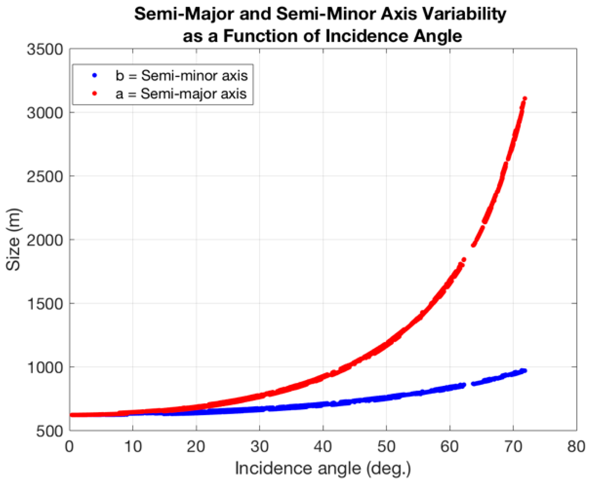
where = 1 defines the first Fresnel zone and is the incidence angle of the reflection, defined as the angle between the normal vector at the specular point and the vector between the specular point and the receiver. For non-inundated vegetated areas or open non-inundated areas, the number of Fresnel zones that contribute to the total power increases, and further n > 1 would need to be considered to perform a rigorous calibration of those signals. The semi-major () and semi-minor () axes of the first Fresnel zone ( = 1) define the resolution of the CYGNSS measurement along the transmitter-to-receiver direction and its perpendicular direction, respectively. The of the forward scattered signals received by CYGNSS can vary between 0° and 70°, giving rise to variation in the size of the first Fresnel zone. Figure 1 shows the incidence angle dependence of the size of those two axes.
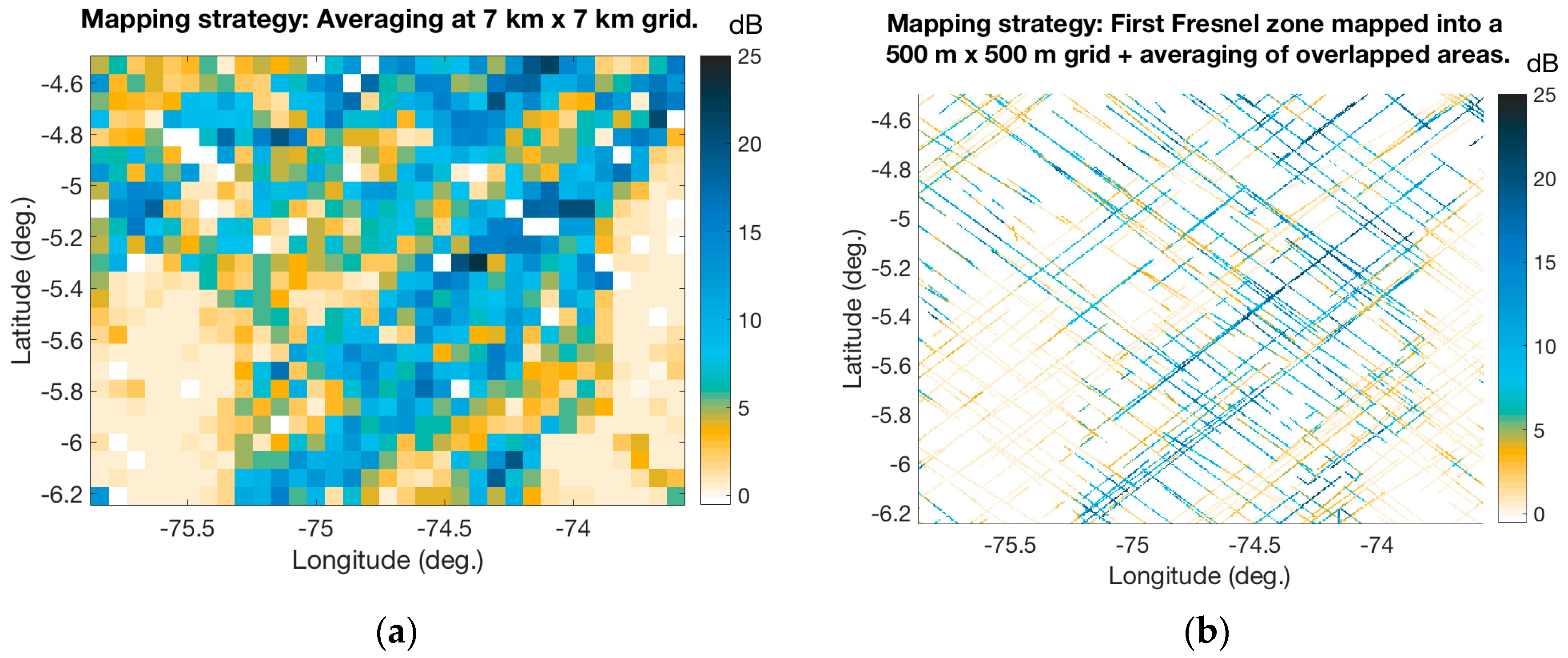
The GNSS-R signals received by CYGNSS are integrated incoherently over a 1 second time window. As a consequence, the first Fresnel zone elongates on the along-track direction due to the distance traveled by the specular point during this integration time (~6 km). Depending on the orientation of the first Fresnel zone ellipse with respect to the along-track direction, the size of the final spatial resolution varies. We selected the case where the semi-major axis aligns with the along-track direction, knowing that the semi-major axis dimension varies from 600 m to 2.8 km for incidence angles below 70° (Figure 1) and that the final size of the ellipse after integration would be 6.6 km and 8.8 km in the along-track dimension. For the same example, the cross-track size would not suffer any elongation and its size would correspond to that of the semi-minor of the first Fresnel zone, varying from 600 m to 1 km depending on incidence angle. The spatial resolution of CYGNSS measurements in that particular case is a variable value between a minimum of 600 m × 6.6 km and a maximum of 1 km × 8.8 km, considering the whole range of incidence angles. In the opposite case, where the semi-minor axis aligns with the along-track direction, the final spatial resolution after integration would be a variable value between a minimum of 600 m × 6.6 km and a maximum of 2.8 km × 7 km, considering the whole range of incidence angles. In order to obtain the GPS scattering area, ellipses were generated based on the semi-major and semi-minor first Fresnel zone dimensions elongated to 6 km in the along-track direction for each single reflection. These ellipses were then mapped onto a fixed 500 m × 500 m grid, and any overlapping areas were averaged. Figure 2 shows an example of the two different gridding strategies considered in this study. The 7 km × 7 km grid contains the average power of all reflection signals with specular points falling within each cell, regardless of the size of the scattering area.
In the case of the 7 km × 7 km fixed grid in Figure 2a, multiple reflections falling within a single grid cell are averaged using a drop-in-the-bucket averaging scheme. In Figure 2b, the 500 m × 500 m grid is fine enough to map the shape of the first Fresnel zone ellipses for each measurement. Visually, the 7 km × 7 km grid shows complete coverage of our study area, however, the contributions to each grid cell value may come from just one specular point, of which the scattering area is not necessarily representative of the entire 7 km × 7 km area (specially for coherent reflections, which have a scattering area that is significantly smaller than that of non-coherent reflections). In contrast, the 500 m × 500 m grid shows large gaps in spatial coverage because it finely maps the first Fresnel zone, which is a better indicator of the surface (inundated wetlands) where most of the scattering is coming from. We therefore opted to use the 500 m × 500 m grid in order to explore the data at its highest spatial resolution, while at the same time focusing on the coherent component of the signal, which is the most relevant to inundated wetlands.
The CYGNSS data calibration is optimized for ocean surfaces. CYGNSS provides a number of variables in its dataset (Level 1, version 2.1): raw_counts corresponds to uncalibrated power values produced by the DDM instrument (DDMI); power_analog in Watts corresponds to the power computed from the raw counts corrected for quantization (L1a calibration); brcs in m2 corresponds to the bistatic radar cross section (BRCS), computed from the DDM power in Watts corrected by the geometry and antenna parameters (L1b calibration); and ddm_nbrcs corresponds to the normalized BRCS computed from the BRCS corrected by the scattering area associated to each specular point. The scattering area pre-computed to normalize the BRCS is only valid for ocean measurements, therefore not suitable for the wetlands application focus of this study. For data over land, both variables power_analog (L1a calibrated data, in Equation 1) and brcs (L1b calibrated data) can be used, since those only consider geometrical and instrument corrections. The expression for L1b calibrated data (brcs variable) is defined in Reference [44] as:
where and correspond to the received power in Watts (power_analog variable in the CYGNSS dataset, L1a calibrated data), and is the BRCS (brcs variable in the CYGNSS dataset, L1b calibrated data).
There are two equivalent ways of obtaining reflectivity with currently available CYGNSS products: (1) using (power_analog dataset) and computing the reflectivity by solving for Γ in Equation (1), or (2) substituting Equation (1) into Equation (4) with and re-arranging the expression to write the as a function of (brcs dataset):
We used brcs data in CYGNSS dataset () to obtain , following Equation (5). The data was filtered following the same quality flag selection as defined in Reference [10]. Table A1 in Appendix A contains a list of the CYGNSS quality flags. In addition, data was filtered to remove noisy DDMs and to remove high-altitude measurements by ensuring the DDM peak fell between delay bin 5 and delay bin 11 with a positive SNR.
2.2. Sensitivity to Inundation
The CYGNSS constellation is composed of eight satellites, each with receivers measuring up to 4 reflections simultaneously. This architecture provides up to 32 simultaneous measurements per second globally. The CYGNSS constellation has an orbit inclination of 35°, limiting global coverage to between ± 38° latitude. This latitudinal coverage, combined with the high spatial resolution and temporal repeatability, make CYGNSS an ideal sensor for monitoring dynamic surface processes such as inundation in tropical wetlands.
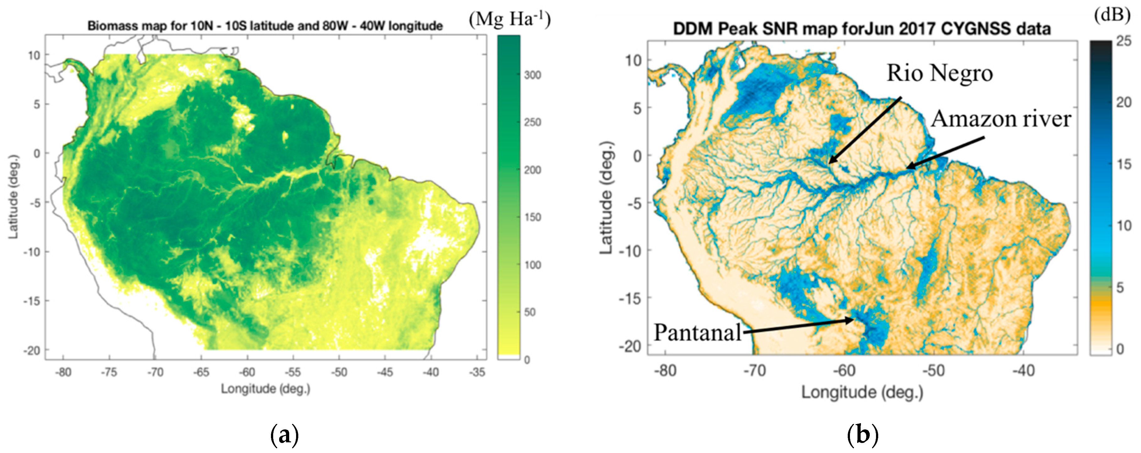
Although CYGNSS was designed for ocean applications, very distinctive signatures are also detected over land where coherent scattering is dominant, such as inundated areas. Figure 3b shows an example of a DDM peak SNR over the Amazon Basin, showing strong returns from rivers and inundated vegetation. The main channel of the Amazon River and Rio Negro (marked in Figure 3b) are clearly delineated, as are many of the large number of tributaries that make up the watershed of the Amazon Basin. Large regions of inundated wetlands (e.g., the Pantanal, marked in Figure 3b) are also apparent at this scale. The high SNR of the CYGNSS signal over inundated areas relates to the highly reflective nature of surface water and to the low surface roughness of these areas. The presence of open water or flooded vegetation (characterized by having very low roughness and high surface reflectance within the first Fresnel zone) causes the reflected signal to be dominated by coherent scattering and increases the received power by 15–20 dB in comparison to other surrounding surfaces with higher surface roughness and minimal or no inundation.
We utilized a biomass map of the Amazon Basin [45] to estimate vegetation density (Figure 3a) and account for CYGNSS data sensitivity to inundation under various levels of vegetation density. Much of the Amazon basin is characterized by dense vegetation, with an average aboveground biomass density over 200 , reaching up to 340 in some areas (darker green in Figure 3a). L-band signals can penetrate through the vegetation canopy to a certain extent, depending on vegetation density and water content, and provide information on whether or not such areas are inundated. Standing water beneath vegetation canopies gives rise to a coherent scattering component that generates a strong return in comparison to non-flooded vegetation or bare soil. Evidence of this is the high return obtained from a large number of tributaries (observed in Figure 3b) that are actually covered by dense vegetation (shown by Figure 3a), and the lower return observed from non-flooded areas surrounding those tributaries.
3. GNSS-R Measurements
This paper defines a new approach to classifying wetland inundation based on GNSS-R observables and ancillary data by employing a classification approach based on the MDTR algorithm. In this section, we define the processing required for the GNSS-R measurements to be comparable to the reference dataset and the different GNSS-R observables built from the measurements to be used in the classification algorithm.
3.1. GNSS-R Measurement Time Averaging
GNSS-R measurements are obtained at a daily rate over the area under study, but in order to compare the results of the classification algorithm to the reference, we performed averaging according to the reference. In this study, we used the PALSAR-2 derived inundation classifications as reference datasets, training, and validation, within the MDTR algorithm scheme to generate the GNSS-R derived inundation classifications. About 80% of the Pacaya-Samiria National Reserve inundates seasonally, with significant portions remaining inundated throughout the year. Maximum inundation occurs during the wet season (November–March). In July and August of 2017 (during the dry season), we conducted an expedition to Pacaya-Samiria to conduct field surveys and collect ground reference data [10]. Detailed vegetation biometry (structure) data were collected for circular plots and along transects. Inundation status was noted and inundation history was inferred based on high water marks remaining on the tree trunks from prior flood seasons. These data were used to generate and validate inundation maps of the entire area using ALOS-2 PALSAR-2 ScanSAR imaging radar mosaics [10]. PALSAR-2 operates at 1.27 GHz (L-band) in wide-swath ScanSAR mode in 14 day cycles, observing our entire study area approximately every ~1–2 months, based on the PALSAR-2 data acquisition plan (http://eorc.jaxa.jp).
The GPS constellation operates at 1.57542 GHz. The similar L-band frequency between CYGNSS and PALSAR-2 ensures that the results are comparable as opposed to for example, using a reference dataset derived from C-band SAR. The associated CYGNSS observables, defined in the following sub-section, were therefore temporally composited and averaged over the respective PALSAR-2 acquisition periods to match the 14-day cycles.
3.2. GNSS-R Observable Definitions
We used the following CYGNSS observables as inputs to the inundation classification algorithm: (1) peak SNR, (2) trailing edge slope (TES), (3) leading edge slope (LES), (4) width of the waveform (), and (5) the generalized linear observable (GLO).
Peak SNR was computed as , where is the maximum value (in raw counts) in a single DDM bin and is the average raw noise counts per bin, which was computed on board the satellite from the first 45 delay rows of the uncompressed DDM (before the data was compressed and sent to the ground). For our study, the peak SNR was corrected using the following coherent assumption: (expressed in linear units). Peak SNR is sensitive to the reflectivity of the observed surfaces; inundated surfaces, covered or not by vegetation, have strong peak SNR as compared to non-inundated surfaces. The strongest peak SNR is observed for open water scenarios.
TES and LES were computed as the slope of the reflectivity delay waveform. The reflectivity delay waveform is the result of integrating Equation 5 with the Doppler domain. TES slope is computed from reflectivity delay waveform values at delay bins m and m + 3, where m corresponds to the position of the peak of the waveform. LES slope is computed from reflectivity delay waveform values at delay bins m and m – 3. was defined as the width of the reflectivity delay waveform at 1/e of the peak value, and the threshold was selected from previous experience, as shown in References [46] or [47]. TES, LES, and are all shape-based observables and are directly linked to the coherency/incoherency of the scattering surface. Inundated surfaces show a more step reflectivity delay waveform, as those surfaces are dominated by coherence scattering. Non-inundated surfaces are dominated by a mix of coherency and incoherence scattering, and are characterized by a reflectivity delay waveform with a smaller slope. In Reference [48], the authors describe the effect of the PRN-dependent autocorrelation function (ACF) deviations on GNSS-R wind speed retrievals. The effect of the ACF deviations for ocean winds speeds under 20 m/s as 2–3 m/s, while the effect for ocean wind speeds of 40 m/s can be 7–8 m/s. The ocean surface produces highly incoherent returns, and the ACF deviations have a significant impact. For the surfaces under consideration (open water—coherent, inundated vegetation—coherently dominated, and non-inundated surfaces—mix of coherency and incoherency), the effect of the ACF deviations was considered negligible for this application.
The GLO observable is based on principal component analysis (PCA) applied to the DDM samples, and was originally defined for the ocean domain in Rodriguez-Alvarez et al. [49]. In that study, the authors showed that the GLO increased the performance of the ocean wind speed retrieval algorithm in comparison to standard observables such as the DDM average (DDMA). The DDMA is the number of DDM samples around the specular point that are averaged together. For example, for a total of samples, DDMA would be defined as , where corresponds, in our case, to the reflectivity samples (Equation (5)) around the specular point. The DDMA observable can be defined by a more general expression, , where the coefficients are set to a constant value, i.e., for DDMA . Here, we propose that the optimal weight coefficients be found, given the characteristics of the data ensemble. The optimal coefficients are found by applying PCA to a data ensemble. This data ensemble requires that the variability of the scenes selected to perform the PCA is representative of the type of area to be described. GLO is sensitive to the reflectivity of the observed surfaces, as peak SNR, i.e., inundated surfaces, covered or not by the vegetation, have high GLO values as compared to non-inundated surfaces. The highest GLO is observed for open water scenarios. The main difference between GLO and peak SNR is that GLO uses bins around the peak to reduce the noise by linearly combining them with optimal coefficients.
In order to make the GLO coefficients general and inclusive of most tropical vegetated river basins, we derived the GLO coefficients by accounting for wide differences in land cover variability, surface conditions, biomass densities, and surface elevation. Therefore, we selected areas around the Congo river basin ([7°S, 12°E]–[5°N, 29°E] and Amazon river basin ([10°S, 77°W]–[2°N, 51°W] latitude–longitude boxes that contain these diverse conditions, and that include and are representative of the area under study (Pacaya-Samiria), and are inclusive of all tropical wetlands around rivers. In order to derive the GLO observable, we used CYGNSS data for those specific Amazon and Congo areas during the high-water season and the low-water season (corresponding to the same dataset used for training our algorithm and defined later in Section 3.2, after Table 2). In a dataset with this level of variability, many contributors can cause differences in the signal received. By observing the impact of standing water on the scattered signal in Figure 3, we assumed that the presence of water above the surface was the primary contributor to changes in the measurements. This assumption was tested later when the impact of the GLO observable in the classification algorithm was evaluated.
In order to build the GLO observables we simplified the study to reflectivity delay waveforms instead of the whole reflectivity DDM (, Equation (5)); given that inundated areas exhibit a coherent dominant forward (specular) scattering, this assumption does not cause a significant loss of information. A delay waveform was obtained by integrating over the Doppler domain (). The PCA was then applied to the samples corresponding to the delay bins m – 3:m + 3 (where m is the position of the maximum power). We retained up to the third principal component to yield GLO 1, GLO 2, and GLO 3 observables. This analysis generated three vectors (aN) of coefficients of size 1 × 7 for each vector, with N corresponding to the first, second, and third principal components, as shown in Table 1.
These coefficients were applied to the waveform samples in order to rotate the samples from the current space to a new orthogonal space. GLO observables were therefore computed as the linear combination of delay waveform samples following Equation (6):
4. Classification Methodology
We developed a new classification methodology using a multiple decision tree randomized structure to construct our MDTR algorithm. This algorithm is similar to Random Forest [50], a machine learning approach that builds multiple decision trees based on different combinations of input variables. The main difference between the Random Forest and the MDTR algorithm is the randomization of the number of inputs, which for Random Forest is fixed to a number selected by the user. The MDTR algorithm employs several GNSS-R observables and ancillary data as inputs, along with reference data for training and validation. We first define the information required by the MDTR algorithm, and then explain the algorithm in detail.
4.1. Datasets
The reference for training and validation used in the MDTR was obtained from PALSAR-2 ScanSAR mosaics that were composited into 14 day cycles, listed in Table 2, and used to derive the inundation maps [10].
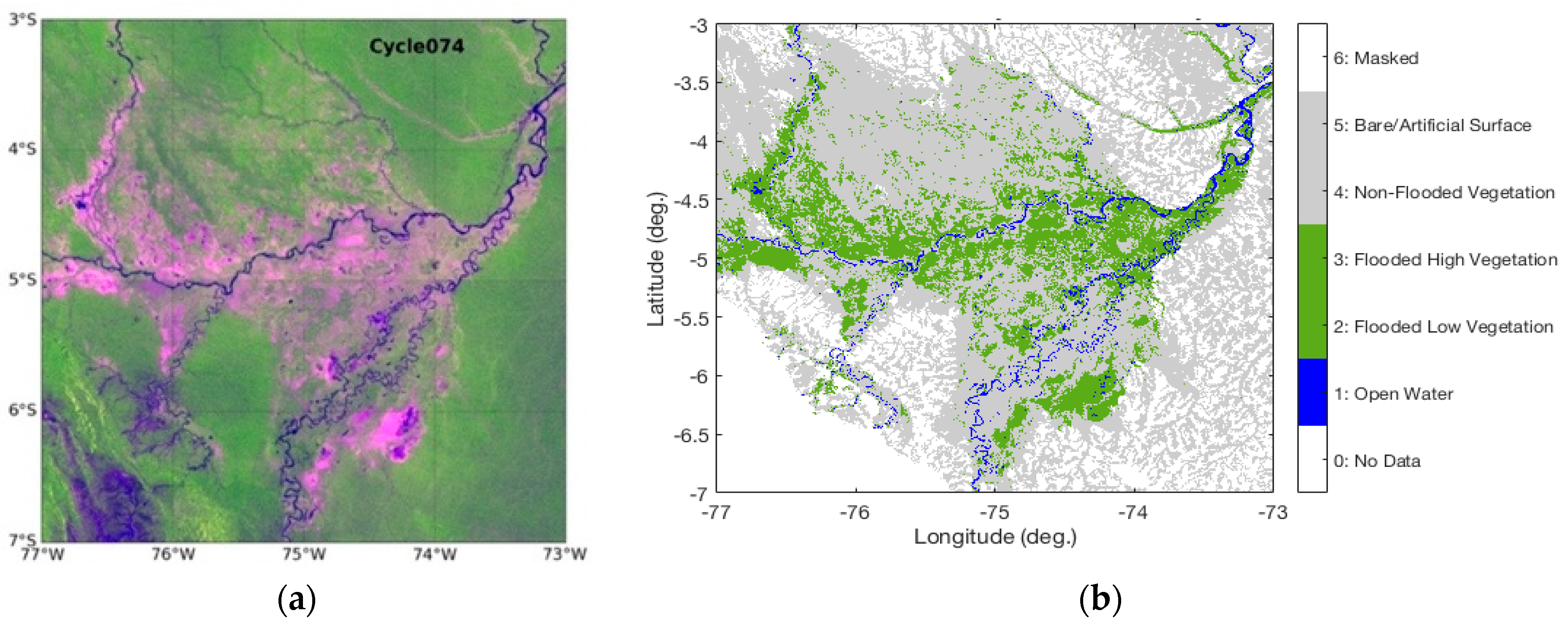
Six of the cycles listed above (71, 77, 79, 83, 85, 88, and 93) were used to train the MDTR algorithm, and two of those cycles (74—end of the high-flood season, and 91—beginning of the high-flood season) were used to evaluate the results. The PALSAR-2-based reference inundation maps were resampled from their original 50 m × 50 m resolution to 0.005° × 0.005° (~500 m × 500 m) to match the CYGNSS grid. Figure 4 shows a false color composite of the PALSAR-2 mosaic corresponding to cycle 74 (8 May to 21 May, end of the high flood season), and the derived PALSAR-2 inundation classification that we used as reference to train the MDTR algorithm. The accuracy of the PALSAR-2 reference maps was determined to be 91.8% [10].
The PALSAR-2 derived inundation classifications had seven classes defined (no data, open water, flooded low vegetation, flooded high vegetation, non-flooded vegetation, bare/artificial surface, and masked areas). In this study, we condensed those seven classes into four: (1) Flooded Vegetation (includes high and low flooded vegetation), (2) Open Water, (3) Non-Flooded vegetation, and (4) Masked areas and regions with no data coverage.
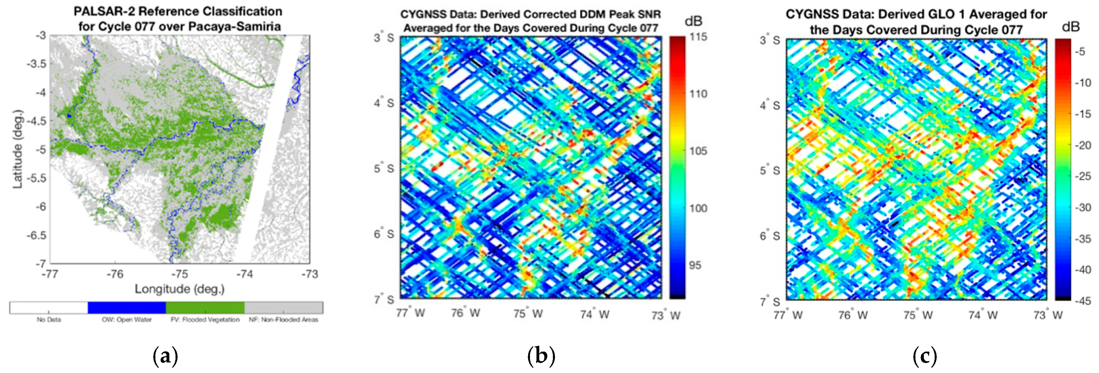
CYGNSS observables were averaged within each corresponding 14 day cycle (Table 2). Figure 5 illustrates two of the observables, DDM corrected peak SNR and GLO 1, for cycles 77 and 93, along with the contemporaneous PALSAR-2-based reference inundation classification maps used for training the MDTR algorithm.
The two cycles selected correspond to a 14-day window (see Table 2) in late June and early July showing high-flood, and a 14 day window in mid–late February showing low-flood. Differences in both peak SNR and GLO 1 can be seen between the two seasons, with higher peak SNR and GLO values during the high-flood than the low-flood period. Non-flooded areas were characterized by the lowest values (on the order of 136–142 dB for peak SNR and —45 to —30 dB for GLO1) while flooded vegetation was characterized by higher values (on the order of 142–148 dB for peak SNR and —30 to —20 dB for GLO1) and open water was characterized by having even higher values (of the order of 148–156 dB for peak SNR and —20 to —5 dB for GLO1).
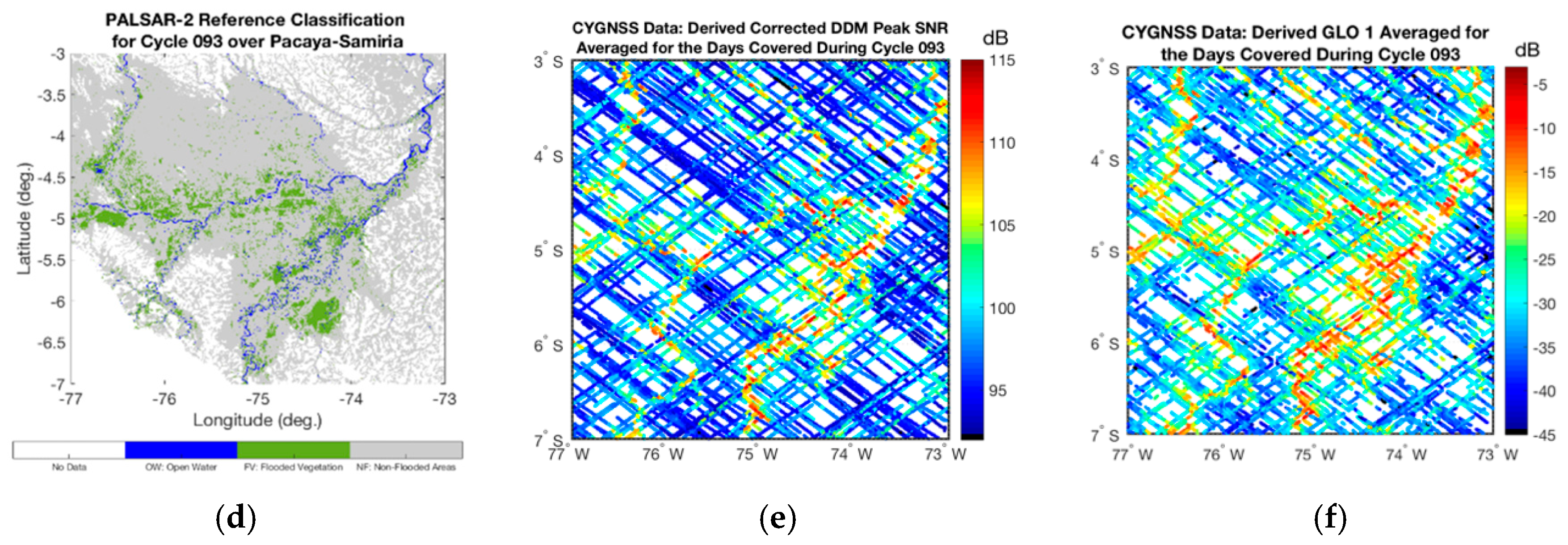
The selection of the GNSS-R observables used by the MDTR algorithm to assess the GNSS-R inundation classification is further discussed in Section 4, analyzing their impact on inundation detection performance. In addition to the GNSS-R observables, the static ancillary datasets were also evaluated to assess their contribution to the classification. These ancillary inputs included: (1) the Shuttle Radar Topographic Mission (SRTM) 90 m resolution global digital elevation model (SRTM90 DEM) [51], Figure 6a, and (2) the Global Forest Watch Aboveground live woody biomass (AGB) density (Mg ha-1) dataset at 30 m resolution for the year 2000 (GFW AGB) [45], Figure 6b.
The SRTM90 DEM provides 90 m resolution data at near-global coverage between 56°S and 60°N, obtained from an 11-day mission in February 2000 from a radar system onboard the Space Shuttle Endeavor. The inaccuracies of the SRTM90 DEM dataset are on the order of 8.2 ± 0.7 m and 6.9 ± 0.5 m, for X-band and C-band respectively, as compared to data from the International GNSS Service (IGS) [52].
GFW AGB was generated from more than 700,000 quality-filtered Geoscience Laser Altimeter System (GLAS) LIDAR observations using allometric equations to estimate AGB based on lidar-derived canopy metrics [45,53]. The global set of GLAS AGB estimates was used to train random forest models that predict AGB based on spatially continuous data and provided global scale estimates. The main uncertainties on the GFW AGB dataset come from errors from allometric equations, the LiDAR based model, and the random forest models. According to their website, the error map for the current version of the biomass density map is not available yet. Both ancillary maps were re-gridded to 0.005° × 0.005° (~500 m × 500 m) to match the CYGNSS data and used as inputs to the classification algorithm.
4.2. Algorithm Training
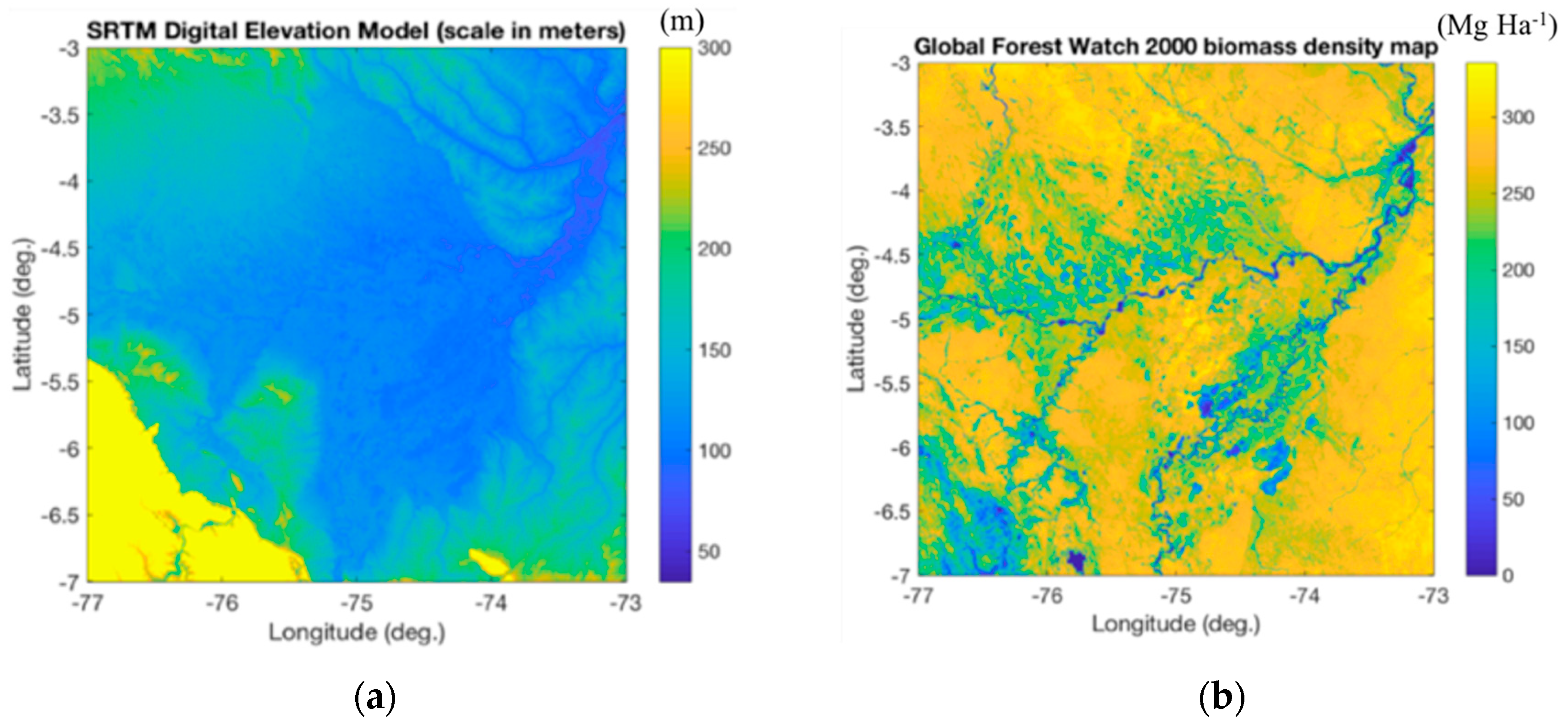
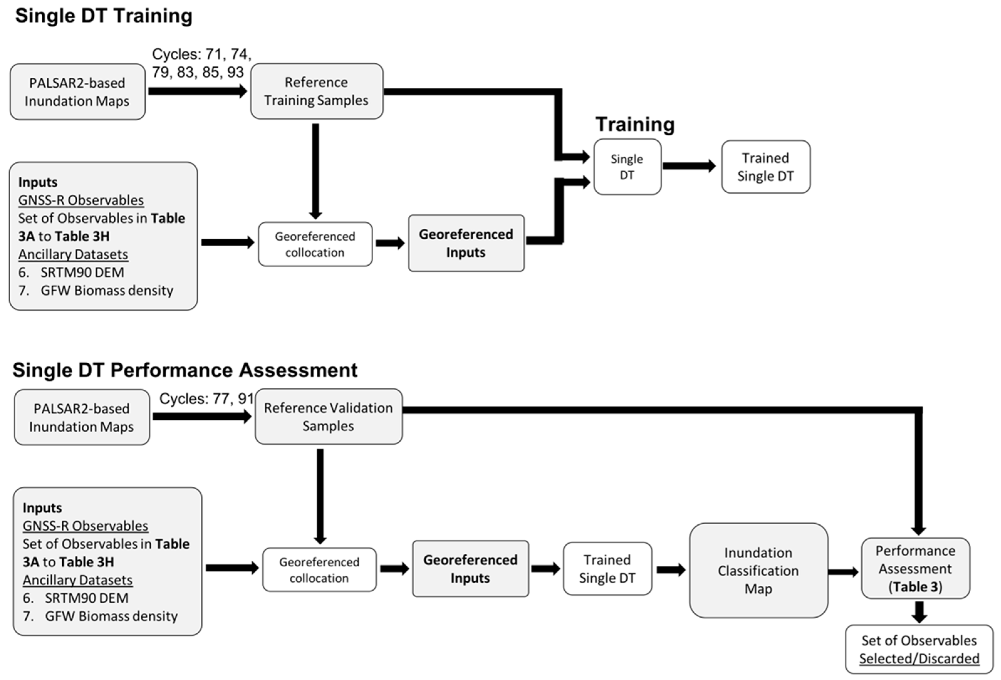
Next, we define the algorithm in more detail, as shown in Figure 7, which summarizes the MDTR algorithm scheme that was implemented in MATLAB.
The input variables correspond to different GNSS-R observables, derived from CYGNSS measurements, and ancillary data (aboveground biomass and elevation), totaling seven different input variables. PALSAR-2-based inundation reference maps were used as reference to train the algorithm and validate the results (referred as PALSAR-2-based reference inundation maps). The MDTR algorithm training scheme (Figure 7) is built through the following steps:
- The reference training samples (cycles 71, 74, 79, 83, 85, and 93 of the PALSAR-2-based inundation reference maps) are randomized in 50 grab samples (each containing 60% of the samples);
- The inputs (5 GNSS-R observables and 2 ancillary datasets) are randomized by selecting 50 different combinations;
- The different combinations of inputs are collocated to each one of the grab samples; and
- The reference grab samples and each combination of collocated inputs are used to train single decision trees (DT).
- Each single DT is based on a standard classification and regression tree (CART) approach for machine learning [54]. A total of 2500 single DT’s are generated, constituting the MDTR algorithm.
The MDTR algorithm validation scheme (Figure 7) is implemented as: (1) the validation reference samples (cycles 77 and 91 of the PALSAR-2-based inundation reference maps) are used to obtain the corresponding geolocated CYGNSS observables; (2) those georeferenced observables are input into the MDTR algorithm; (3) to classify a given grid cell, a total of 2500 outputs are evaluated; (4) the grid cell is assigned the class that is identified most often by the ensemble of decision trees, generating the final GNSS-R inundation classification map; and (5) the classification outputs are compared to the validation reference samples to assess the performance of the GNSS-R inundation classification obtained from the MDTR algorithm.
4.3. Performance Validation and Results
In a trade assessment, we first determine the GNSS-R observables and ancillary datasets associated with improving our inundation classification. We discard those observables that diminish accuracy. Here, we assessed the classification accuracy of each individual observable for the three classes defined (Open Water (OW), Flooded Vegetation (FV), and Non-Flooded Vegetation (NF)). We built a single decision tree (DT) from each observable and one or two of the ancillary datasets (DEM and biomass). Each single DT was constructed following a standard CART based classification algorithm [54]. Figure 8 explains the methodology followed to train and validate a single DT.
Figure 8 shows the methodology followed to train and validate the single DTs built from the GNSS-R observables and ancillary datasets listed in Table 3. We started by building the classification algorithm with the most commonly used observables (corrected peak SNR and TES) and the ancillary datasets (DEM and biomass). We then assessed additional observables and identified those that improved the classification accuracy. The single DTs were trained (using cycles 71, 77, 79, 83, 85, 88, and 93), and then their performance was assessed using independent data from cycles 74 and 91 (end of high-flood season and beginning of high-flood season, respectively). Various combinations of inputs (corrected peak SNR, TES, LES, ∆, GLO 1, GLO 2, GLO 3, SRTM90 DEM, GFW AGB) were tested, with the aim of assessing the impact of each one on classification performance. Confusion matrices summarizing the results of each of these iterations are shown in Table 3, focusing on three classes: OW, FV, and NF.
We first investigated corrected peak SNR since it is the most widely used observable, as in References [30,32], along with DEM and biomass information. Table 3A shows the performance of a single DT built using corrected peak SNR + SRTM90 DEM + GFW biomass density as inputs. Table 3A shows that corrected peak SNR provided high classification accuracy for the NF class (93.63%) but low accuracy for both OW and FV (both <60%). The next step was to investigate the TES observable along with the DEM and biomass ancillary datasets, as summarized in Table 3B. Results indicate that the TES observable improved the classification of OW by approximately 4% and FV by about 1.5 % when compared to corrected peak SNR. We then assessed classification accuracy with both corrected peak SNR and TES observables, together with the two ancillary datasets. The results are summarized in Table 3C, and indicate that a higher classification accuracy was achieved than with any of the previous combinations of inputs (Table 3A,B). OW was classified with 64% accuracy, FV with 59%, and NF with 93%, resulting in a 5.3% increase for OW and 5% for FV as compared to Table 3A,B.
Next, we analyzed the contribution of the ancillary datasets towards classification accuracy. Table 3D,E shows the classification accuracy results using both corrected peak SNR and TES and a single ancillary dataset: SRTM90 DEM and then biomass density, respectively. A comparison of Table 3D with Table 3E shows that the SRTM90 DEM contributed overall less to classification accuracy than biomass. For example, classification accuracy of OW was 14% higher with biomass than with the SRTM90 DEM. The low contribution of the SRTM90 DEM was likely because the Pacaya-Samiria region is relatively flat, however, its inclusion is important in areas with large topographic variability.
Table 3F illustrates the impact of including LES, , and GLO 1 to the list of inputs, together with corrected peak SNR, TES, DEM, and biomass information (Table 3C). We did not include rows in the Table for each of them because their individual impact to the classification is minimal. Instead we assessed the overall improvement associated with LES, , and GLO 1 collectively (Table 3F). Even though the individual assessment is not included in Table 3, we summarize it here: LES observable did not contribute to any further separability in any class, but since it did not negatively impact classification performance it was still considered in the final classification algorithm. The observable helped improve classification of OW by about 1.5% and classification of FV by about 1.3%. Finally, there was an improvement of 0.7% for OW after adding GLO 1. Comparison of Table 3C and Table 3F highlights the overall improvement in accuracy upon inclusion of these three observables, which was about +2% for OW, +1% for FV, and +1% for NF. Table 3G,H shows the effect of adding GLO 2 and GLO 3, respectively. In comparing Table 3G and Table 3H to Table 3F, observables GLO 2 and GLO 3 added ambiguity to the results and were not likely to be sensitive to inundation, since adding them worsened the classification performance (−10% for the OW class in both cases, and –10–30% for FV). In Section 3.1, we stated our assumption that the GLO 1 observable would be able to capture most of the information related to inundation conditions, and that it would be the factor most strongly affecting the shape and strength of the measurement. The classification results in Table 3F, Table 3G and Table 3H for observables GLO 1, GLO 2, and GLO 3 respectively, show that the dependence of the signal on inundation was well captured by the first principal component alone. Consequently, GLO2 and GLO3 were not selected in the final classification algorithm.
In summary, we trained single DT’s on different combinations of observables and ancillary datasets and assessed the performance of those against the PALSAR-2-based inundation reference maps for cycles 74 and 91. We started with the most commonly used observables (corrected peak SNR and TES) and ancillary datasets (DEM and biomass), and we then added additional observables, retaining only those that increased classification accuracy. The results in Table 3A–H indicate that adding TES, LES, ∆, and GLO 1 to peak SNR improved the classification accuracy for OW and FV. Overall, NF areas were classified with high accuracy (≥93%). Misclassifications of OW and FV as NF most likely occurred because of the surface conditions of those particular observations. A lower percentage of OW or FV within the scattering area caused the scattering to become more incoherent, and the power level, along with other observable parameters, become closer to NF. A comparison of Table 3A (corrected peak SNR + SRTM90 DEM + GFW biomass density) and Table 3F (corrected peak SNR + TES + LES + ∆ + GLO 1 + SRTM90 DEM + GFW biomass density) indicates that, for the latter, there was an overall improvement in classification accuracy of 7.4% for OW and 6.5% for FV, illustrating the value of using multiple observables in the classification algorithm.
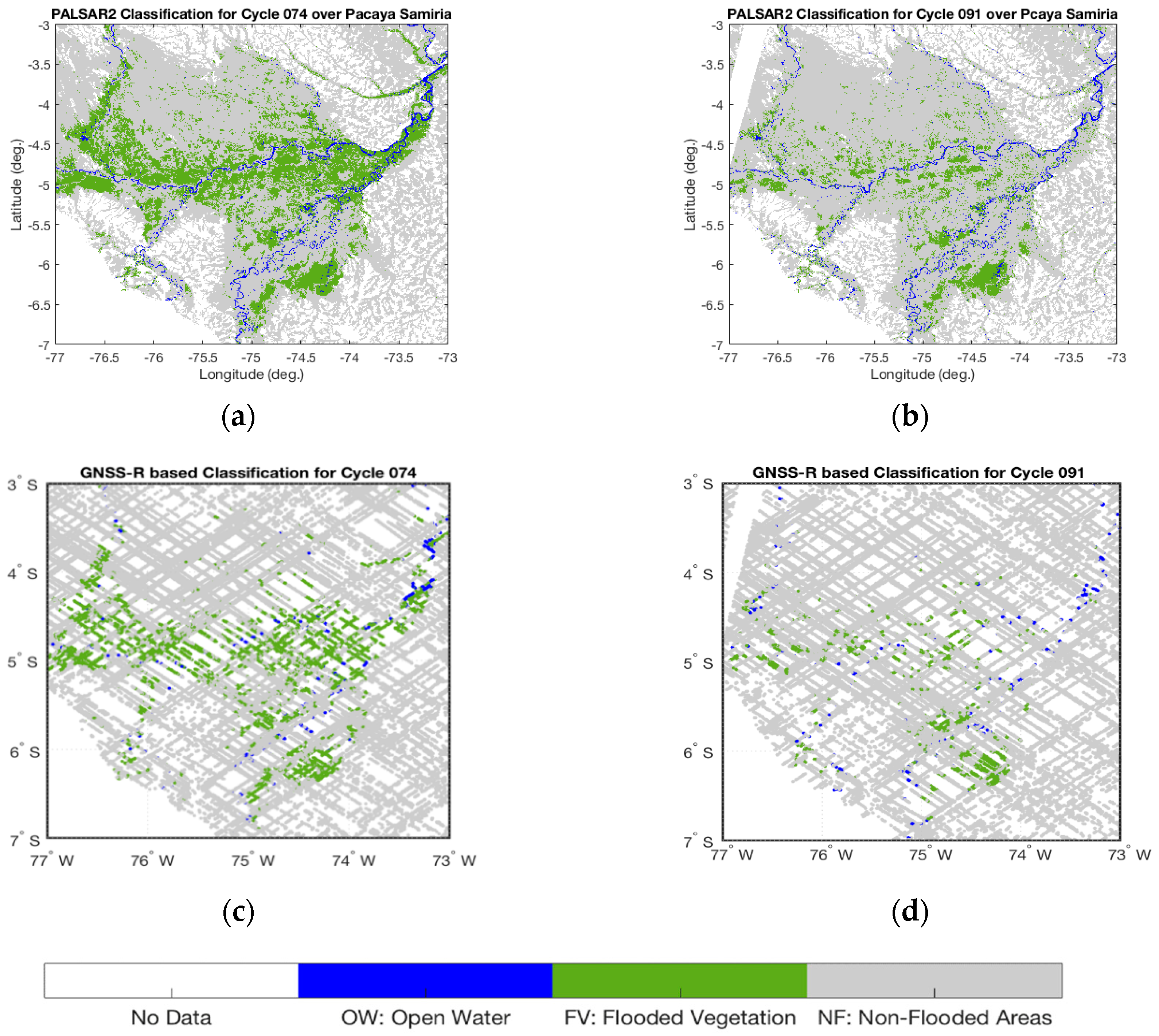
After exploring the contribution of the different observables towards the performance of the single DTs, we implemented the MDTR algorithm, described in Section 3.2, with the selected inputs derived from this explorative study (Table 3F): corrected peak SNR, TES, LES, Δ, GLO 1, SRTM90 DEM, and GFW biomass density, following the flowchart in Figure 4. Figure 9 and Table 4 summarize the results of our GNSS-R inundation classification obtained from the MDTR algorithm.
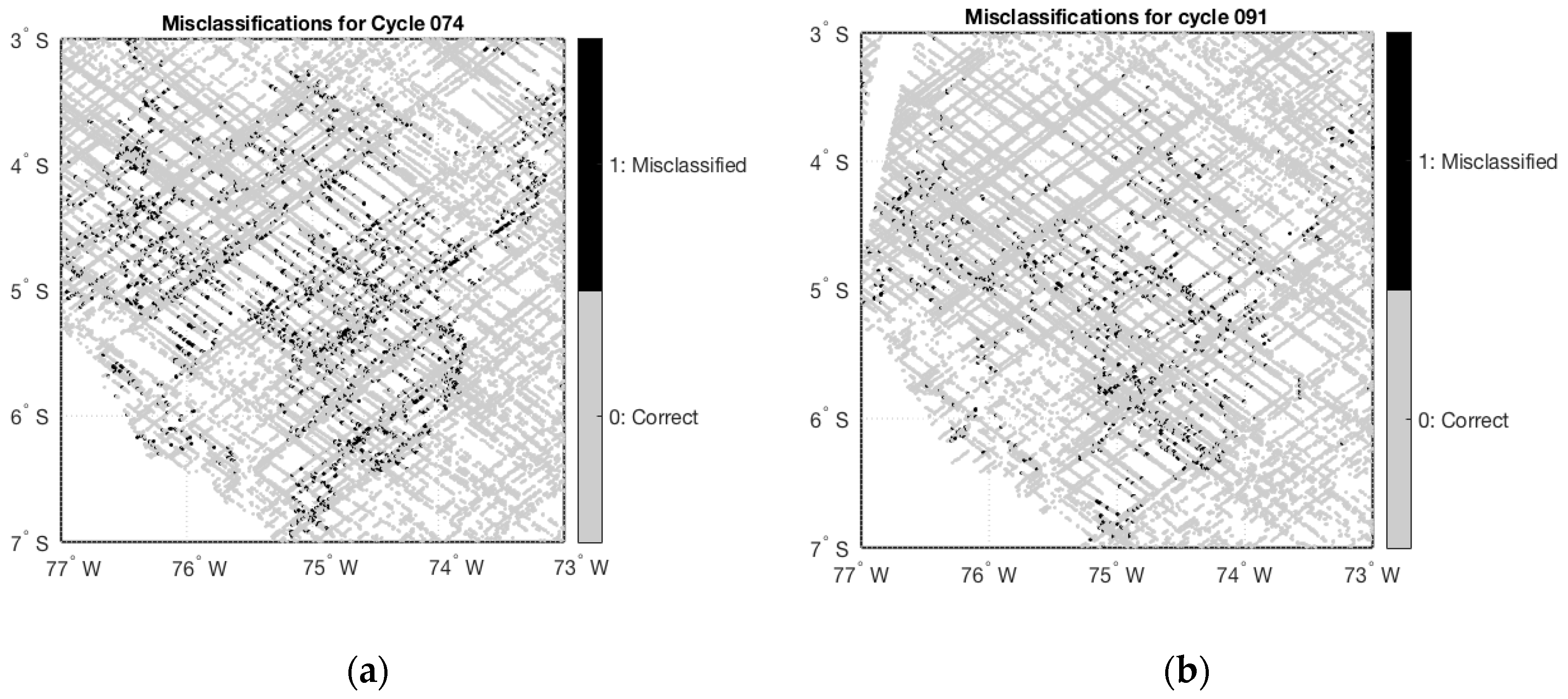
Figure 9 illustrates the classification results of the GNSS-R derived inundation classifications validated using data from cycle 74 (left column) and cycle 91 (right column). Figure 10 shows the location of the misclassifications for both cycles 074 and 091.
Figure 10 shows that most of the misclassifications occurred around the areas of flooded vegetation. The accuracy results of the GNSS-R inundation classification obtained from the MDTR algorithm are assessed in Table 4.
FV had a classification accuracy of 69%, demonstrating the ability of the forward scattered L-band signal to penetrate through the vegetation canopy and detect inundated vegetation. OW had an accuracy of 86%, despite the narrowness of the river in the study area relative to the footprint size of the CYGNSS reflection. The roughness of the surface had an impact on the total power received (a rougher and larger scattering area yields a lower SNR and the signal becomes incoherent), and hence the contribution of the river was attenuated in cases where it covered only a small part of the scattering area and the specular point fell far from it. Finally, NF classification accuracy was 99.7%, however, a high percentage of OW and FV pixels were misclassified as NF, which can also be observed in the location of the misclassifications shown in Figure 10. This is likely explained by the presence of areas of OW or FV that were small relative to the size of the CYGNSS footprint, resulting in an incoherent signal (larger footprint) and reducing the SNR to that of NF. This effect was more noticeable for FV, because the vegetation contributed to the loss of coherency.
Table 4 also shows that the classification with the MDTR algorithm resulted in overall better results than a single DT (Table 3F, highlighted in bold black). A comparison between the two approaches indicates that the MDTR algorithm improved classification accuracy of OW by 20%, FV by 9%, and NF by 5% when compared to a single DT.
5. Discussion
The L-band PALSAR-2 radar imagery provides a measurement suitable for direct comparison with the L-band GPS L1 band measurements of CYGNSS. However, our results are limited by the accuracy of the PALSAR-2 reference maps, which was previously determined to have an overall accuracy of 91.8% [10]. There may also be differences due to daily variability that is not captured by PALSAR-2 and that has been averaged by the CYGNSS measurements to match the 14-day cycle characteristic of the PALSAR-2 mosaics. In addition, the ancillary datasets have associated uncertainties that may also affect the final performance of the MDTR classification algorithm. The uncertainty of the ancillary datasets is assumed to be small compared to the uncertainties derived from the GNSS-R measurements.
The main source of misclassification is the size of the scattering surface. In this study, we assumed that the size of the first Fresnel zone represents the area contributing to the received power. The less coherent the scattering, the bigger this area becomes. A deeper study is needed to look into a more adequate representation of the scattering zone size, and a more detailed analysis of what the reflected power properties are as a function of the scattering zone size and the elements within this zone. Better understanding is needed of the effect of having a small portion of standing water within a scattering area, and how the position of the standing water affects the resulting reflected power as a function of its proximity to the specular point. In this study, we observed that a small percentage of open water or flooded vegetation within the scattering area but away from the specular point, produced scattering properties closer to non-flooded conditions. In general, more studies are needed to understand the scattered power resulting from a non-homogeneous surface with variable scattering properties derived from differently located surface characteristics within the scattering surface.
6. Conclusions
We successfully applied an inundation classification through a new implementation strategy, based on a multiple decision tree randomized (MDTR) algorithm and using CYGNSS data over seasonally inundated wetlands in the Pacaya-Samiria region of the Peruvian Amazon. Training and validation data were obtained from PALSAR-2-based reference inundation maps that were developed and evaluated with ground measurements collected during a field campaign in the region [10].
Different combinations of GNSS-R observables were analyzed by building single decision trees (single DTs) from a standard CART classification algorithm (Table 3) and analyzing relative performance, selecting those that increased classification accuracy (corrected peak SNR, TES, LES, ∆, GLO 1) and discarding those that decreased it (GLO 2 and GLO 3). Among the observables selected, the combination of TES and corrected peak SNR resulted in a higher classification accuracy than using corrected peak SNR alone, with an increase of 5.3% for OW and 5% for FV. Observables LES, ∆, and GLO 1 together had lower impact (2% for OW, 1.5% for FV, and 1% for NF), but still contributed towards increasing classification accuracy. The combination of corrected peak SNR, TES, LES, ∆, GLO 1 and the ancillary datasets (DEM and biomass) into a single DT resulted in a classification accuracy of 60% for OW, 60.5% for FV, and 94.7% for NF.
Once the set of GNSS-R observables was selected (corrected peak SNR, TES, LES, ∆, GLO 1), a GNSS-R-based inundation classification was generated using the MDTR algorithm. The randomization (input and data samples) and the extension (2500 trained single DT CART-based trees) of our algorithm allowed an increase in classification performance. The classification accuracy obtained was 86.5% for OW, 69% for FV, and 99% for NF. The use of the MDTR algorithm scheme versus the single DT scheme resulted in an increase of 26.5% for OW, 9% for FV, and 4.3% for NF.
The work presented here demonstrates the utility of GNSS-R observables from CYGNSS data and ancillary datasets to characterize wetland inundation. Bistatic radar signals from GPS satellites or other signals of opportunity have great potential to fill observational gaps from other sensors, and potentially enhance and extend their utility for characterization of these critical biomes.
Author Contributions
Conceptualization, N.R.-A. and E.P.; Formal analysis, N.R.-A.; Funding acquisition, E.P.; Investigation, N.R.-A., K.J., E.P. and K.C.M.; Methodology, N.R.-A. and E.P.; Project administration, E.P.; Software, N.R.-A.; Supervision, E.P.; Validation, N.R.-A. and K.J.; Visualization, N.R.-A.; Writing—original draft, N.R.-A.; Writing—review & editing, N.R.-A., K.J., E.P. and K.C.M.
Funding
This research was funded by the Jet Propulsion Laboratory, under the R&TD program. The research carried out at the Jet Propulsion Laboratory (JPL), California Institute of Technology, was supported under a contract with the National Aeronautics and Space Administration (NASA).
Acknowledgments
Portions of this work were conducted within the framework of the ALOS Kyoto & Carbon Initiative. PALSAR-2 data were provided by JAXA/EORC. Portions of this effort were supported by the NASA Earth and Space Science Fellowship (NESSF) program under grant 80NSSC17K0387. We would like to thank JAXA/EORC and NESSF for the contribution to make this work complete. Also, we would like to thank CYGNSS mission for providing L1 dataset, v.2.1.
Conflicts of Interest
The authors declare no conflict of interest.
Appendix A. Additional CYGNSS Dataset Information

Table A1.
CYGNSS L1 data quality flags used in this study [10].
Table A1.
CYGNSS L1 data quality flags used in this study [10].
| Quality Flag | Flagged in Analysis |
|---|---|
| Poor Overall Quality | No |
| S Band Powered Up | Yes |
| Small Spacecraft Attitude Error | No |
| Large Spacecraft Attitude Error | Yes |
| Blackbody DDM | Yes |
| DDMI Reconfigured | Yes |
| Spacewire CRC Invalid | Yes |
| DDM is Test Patten | Yes |
| Channel Idle | Yes |
| Low Confidence DDM Noise Floor | No |
| SP Over Land | No |
| SP Very Near Land | No |
| SP Near Land | No |
| Large Step Noise Floor | No |
| Direct Signal in DDM | Yes |
| Low Confidence GPS EIRP Estimate | Yes |
| RFI Detected | Yes |
| BRCS DDM SP Bin Delay Error | No |
| BRCS DDM SP Bin Doppler Error | No |
| Negative BRCS Value Used for NRBCS | No |
| GPS PVT SP3 Error | No |
| SP Non Existent Error | Yes |
| BRCS LUT Range Error | No |
| Antenna Data LUT Range Error | No |
| Blackbody Framing Error | Yes |
| FSW Comp Shift Error | No |
References
- Matthews, E. Atmospheric Methane: Its Role in the Global Environment; Khalil, M.A.K., Ed.; Springer: Berlin, Germany, 2000; pp. 202–233. [Google Scholar]
- Ciais, P.; Sabine, C.; Bala, G.; Bopp, L.; Brovkin, V.; Canadell, J.; Chhabra, A.; DeFries, R.; Galloway, J.; Heimann, M.; et al. Carbon and Other Biogeochem Cycles. In Climate Change 2013: The Physical Science Basis; Stocker, T.F., Qin, D., Plattner, G.-K., Tignor, M., Allen, S.K., Boschung, J., Nauels, A., Xia, Y., Bex, V., Midgley, P.M., Eds.; Cambridge University Press: Cambridge, UK; New York, NY, USA, 2013. [Google Scholar]
- Nisbet, E.G.; Dlugokencky, E.J.; Bousquet, P. Methane on the rise—Again. Science 2014, 343, 493–495. [Google Scholar] [CrossRef]
- Page, S.E.; Rieley, J.O.; Banks, C.J. Global and regional importance of the tropical peatland carbon pool. Glob. Chang. Biol. 2011, 17, 798–818. [Google Scholar] [CrossRef] [Green Version]
- Bridgham, S.D.; Johnson, C.A.; Pastor, J.; Updegraff, K. Potential Feedbacks of northern wetlands to climate change. Bioscience 1995, 45, 262–274. [Google Scholar]
- Alsdorf, D.E.; Lettenmaier, D.P.; Vorosmarty, C.; The NASA Surface Water Working Group. The need for global, satellite-based observations of terrestrial surface waters. Eos Trans. AGU 2003, 84, 269–280. [Google Scholar] [CrossRef]
- Frankenberg, C.; Meirink, J.F.; van Weele, M.; Platt, U.; Wagner, T. Assessing methane emissions from global space-borne observations. Science 2005, 308, 1010–1014. [Google Scholar] [CrossRef] [PubMed]
- Prigent, C.; Papa, F.; Aires, F.; Rossow, W.B.; Matthews, E. Global inundation dynamics inferred from multiple satellite observations, 1993–2000. J. Geophys. Res. 2007, 112. [Google Scholar] [CrossRef] [Green Version]
- Schroeder, R.; McDonald, K.C.; Chapman, B.D.; Jensen, K.; Podest, E.; Tessler, Z.D.; Bohn, T.J.; Zimmermann, R. Development and evaluation of a multi-year fractional surface water data set derived from active/passive microwave remote sensing data. Remote Sens. 2015, 7, 16688–16732. [Google Scholar] [CrossRef]
- Jensen, K.; McDonald, K.; Podest, E.; Rodriguez-Alvarez, N.; Horna, V.; Steiner, N. Assessing L-band GNSS-reflectometry and imaging radar for detecting sub-canopy inundation dynamics in a tropical wetlands complex. Remote Sens. 2018, 10. [Google Scholar] [CrossRef]
- Di Vittorio, C.A.; Georgakakos, A.P. Land cover classification and wetland inundation mapping using MODIS. Remote Sens Environ. 2018, 204, 1–17. [Google Scholar] [CrossRef]
- Li, L.; Vrieling, A.; Skidmore, A.; Wang, T.; Munoz, A.-R.; Turak, E. Evaluation of modis spectral indices for monitoring hydrological dynamics of a small, seasonally-flooded wetland in southern Spain. Wetlands 2015, 35, 851–864. [Google Scholar] [CrossRef]
- Chen, Y.; Huang, C.; Ticehurst, C.; Merrin, L.; Thew, P. An evaluation of MODIS daily and 8-day composite products for floodplain and wetland inundation mapping. Wetlands 2013, 33, 823–835. [Google Scholar] [CrossRef]
- Touzi, R.; Deschamps, A.; Rother, G. Wetland characterization using polarimetric radarsat-2 capability. Can. J. Remote Sens. 2007, 33, S56–S67. [Google Scholar] [CrossRef]
- Hess, L.L.; Melack, J.M.; Simonett, D.S. Radar detection of flooding beneath the forest canopy: A review. Int. J. Remote Sens. 1990, 11, 1313–1325. [Google Scholar] [CrossRef]
- Gallant, A.L.; Kaya, S.G.; White, L.; Brisco, B.; Roth, M.F.; Sadinski, W.; Rover, J. Detecting emergence, growth, and senescence of wetland vegetation with polarimetric synthetic aperture radar (SAR) data. Water 2014, 6, 694–722. [Google Scholar] [CrossRef]
- White, L.; Brisco, B.; Pregitzer, M.; Tedford, B.; Boychuk, L. Radarsat-2 beam mode selection for surface water and flooded vegetation mapping. Can. J. Remote Sens. 2014, 40, 135–151. [Google Scholar]
- Chapman, B.; McDonald, K.; Shimada, M.; Rosenqvist, A.; Schroeder, R.; Hess, L. Mapping Regional Inundation with Spaceborne L-Band SAR. Remote Sens. 2015, 5, 5440–5470. [Google Scholar] [CrossRef]
- Papa, F.; Prigent, C.; Aires, F.; Jimenez, C.; Rossow, W.B.; Matthews, E. Interannual variability of surface water extent at the global scale, 1993–2004. J. Geophys. Res. 2010, 115. [Google Scholar] [CrossRef] [Green Version]
- Jensen, K.; McDonald, K.C. Surface water microwave product series (SWAMPS) version 3: A near-real time and 25-year historical global inundated area fraction time series from active and passive microwave remote sensing. IEEE Geosci. Remote Sens. Lett. 2019. [Google Scholar] [CrossRef]
- Lehner, B.; Doll, P. Development and validation of a global database of lakes, reservoirs and wetlands. J. Hydrol. 2004, 296, 1–22. [Google Scholar] [CrossRef]
- Brakenridge, R.; Anderson, E. MODIS-based flood detection, mapping and measurement: The potential for operational hydrological applications. Transbound. Floods Reduc. Risks Through Flood Manag. 2006. [Google Scholar] [CrossRef]
- Hess, L.L.; Melack, J.M.; Novo, E.M.; Barbosa, C.C.; Gastil, M. Dual-season mapping of wetland inundation and vegetation for the central Amazon basin. Remote Sens. Environ. 2003, 87, 404–428. [Google Scholar] [CrossRef]
- Betbeder, J.; Gond, V.; Frappart, F.; Bagdhadi, N.; Briant, G.; Bartholomé, E. Mapping of Central Africa Forested Wetlands Using Remote Sensing. IEEE J. Sel. Top. Appl. Earth Obs. Remote Sens. 2014, 7, 531–542. [Google Scholar] [CrossRef] [Green Version]
- Le Toan, T.; Ribbes, F.; Wang, L.; Floury, N.; Ding, K.H.; Kong, J.A.; Fujita, N.; Kurosu, T. Rice crop mapping and monitoring using ERS-1 data based on experiment and modeling results. IEEE Trans. Geosci. Remote Sens. 1997, 35, 41–56. [Google Scholar] [CrossRef]
- Wang, Y.; Weinacker, H.; Koch, B. A LIDAR point cloud-based procedure for vertical canopy structure analysis and 3D single tree modelling in forest. Sensors 2008, 8, 3938–3951. [Google Scholar] [CrossRef]
- Chapman, B.; Celi, J.; Hamilton, S.; McDonald, K. Validation of forested inundation extent revealed by L-band polarimetric and interferometric SAR data. In Proceedings of the International Geoscience and Remote Sensing Society Symposium, Quebec, Canada, 13–18 July 2014. [Google Scholar]
- Ruf, C.S.; Gleason, S.; Jelenak, Z.; Katzberg, S.; Ridley, A.; Rose, R.; Scherrer, J.; Zavorotny, V.U. The CYGNSS nanosatellite constellation hurricane mission. In Proceedings of the 2012 IEEE International Geoscience and Remote Sensing Symposium, Munich, Germany, 22–27 July 2012; pp. 214–216. [Google Scholar]
- Ruf, C.; Unwin, M.; Dickinson, J.; Rose, R.; Rose, D.; Vincent, M.; Lyons, A. CYGNSS: Enabling the Future of Hurricane Prediction [Remote Sensing Satellites]. IEEE Geosci. Remote Sens. Mag. 2013, 1, 52–67. [Google Scholar] [CrossRef]
- Nghiem, S.V.; Zuffada, C.; Shah, R.; Chew, C.; Lowe, S.T.; Mannucci, A.J.; Cardellach, E.; Brakenridge, G.R.; Geller, G.; Rosenqvist, A. Wetland monitoring with global navigation satellite system reflectometry. Earth Space Sci. 2016, 4, 16–39. [Google Scholar] [CrossRef]
- Foti, G.; Gommenginger, C.; Jales, P.; Unwin, M.; Shaw, A.; Robertson, C.; Rosello, J. Spaceborne gnss reflectometry for ocean winds: First results from the UK TechDemosat-1 mission. Geophys. Res. Lett. 2015, 42, 5435–5441. [Google Scholar] [CrossRef]
- Zuffada, C.; Chew, C.; Nghiem, S.V. Global navigation satellite system reflectometry (GNSS-R) algorithms for wetland observations. In Proceedings of the 2017 IEEE International Geoscience and Remote Sensing Symposium (IGARSS), Fort Worth, TX, USA, 23–28 July 2017; pp. 1126–1129. [Google Scholar]
- Chew, C.; Reager, J.T.; Small, E. CYGNSS data map flood inundation during the 2017 Atlantic hurricane season. Sci. Rep. 2018. [Google Scholar] [CrossRef]
- Wan, W.; Liu, B.; Zeng, Z.; Chen, X.; Wu, G.; Xu, L.; Chen, X.; Hong, Y. Using CYGNSS data to monitor China’s flood inundation during typhoon and extreme precipitation events in 2017. Remote Sens. 2019, 11. [Google Scholar] [CrossRef]
- Rosenqvist, A.; Shimada, M.; Suzuki, S.; Ohgushi, F.; Tadono, T.; Watanabe, M.; Tsuzuku, K.; Watanabe, T.; Kamijo, S.; Aoki, E. Operational performance of the ALOS global systematic acquisition strategy and observation plans for ALOS-2 PALSAR-2. Remote Sens. Environ. 2014, 155, 3–12. [Google Scholar] [CrossRef]
- Zavorotny, V.U.; Voronovich, A.G. Scattering of GPS signals from the ocean with wind remote sensing application. IEEE Trans. Geosci. Remote Sens. 2000, 38, 951–964. [Google Scholar] [CrossRef]
- Voronovich, A.G.; Zavorotny, V.U. Bistatic radar equation for signals of opportunity revisited. IEEE Trans. Geosci. Remote Sens. 2018, 56, 1959–1968. [Google Scholar] [CrossRef]
- Weiqiang, L.; Cardellach, E.; Fabra, F.; Rius, A.; Ribó, S.; Martín-Neira, M. First spaceborne phase altimetry over sea ice using TechDemoSat-1 GNSS-R signals. Geophys. Res. Lett. 2017, 44, 8369–8376. [Google Scholar] [CrossRef]
- Loria, E.; O’Brien, A.; Gupta, I.J. Detection & Separation of Coherent Reflections in GNSS-R Measurements Using CYGNSS Data. In Proceedings of the IGARSS 2018—2018 IEEE International Geoscience and Remote Sensing Symposium, Valencia, Greece, 22–27 July 2018; pp. 3995–3998. [Google Scholar]
- Roo, R.D.D.; Ulaby, F.T. Bistatic specular scattering from rough dielectric surfaces. IEEE Trans. Antennas Propag. 1994, 42, 220–231. [Google Scholar] [CrossRef]
- Ulaby, F.T.; Long, D.G. Microwave Radar and Radiometric Remote Sensing; University of Michigan Press: Michigan, MI, USA, 2014. [Google Scholar]
- Beckmann, P.; Spizzichino, A.E. The Scattering of Electromagnetic Waves from Rough Surfaces; Pergamon Press: Oxford, UK, 1963. [Google Scholar]
- Ghasemi, A.; Abedi, A.; Ghasemi, F. Propagation Engineering in Wireless Communications; Springer: New York, NY, USA, 2011. [Google Scholar]
- Ruf, C.; Scherrer, J.; Rose, R.; Provost, D. Algorithm Theoretical Basis Document Level 1B DDM Calibration. Tech. Rep. 2014. Available online: https://clasp-research.engin.umich.edu/missions/cygnss/reference/ATBD%20L1B%20DDM%20Calibration%20R1.pdf (accessed on 3 May 2018).
- GlobalForestWatch. Global Forest Watch Aboveground Live Woody Biomass Density Dataset. Available online: http://data.globalforestwatch.org/datasets/8f93a6f94a414f9588ce4657a39c59ff_1 (accessed on 3 May 2018).
- Rodriguez-Alvarez, N.; Akos, D.M.; Zavorotny, V.U.; Smith, J.A.; Camps, A.; Fairall, C.W. Airborne GNSS-R Wind Retrievals Using Delay–Doppler Maps. IEEE Trans. Geosci. Remote Sens. 2013, 51, 626–641. [Google Scholar] [CrossRef]
- Carreno-Luengo, H.; Lowe, S.; Zuffada, C.; Esterhuizen, S.; Oveisgharan, S. Spaceborne GNSS-R from the SMAP mission: first assessment of polarimetric scatterometry over land and cryosphere. Remote Sens. 2017, 9. [Google Scholar] [CrossRef]
- Weiqiang, L.; Cardellach, E.; Fabra, F.; Ribó, S.; Rius, A. Effects of PRN-dependent ACF deviations on GNSS-R wind speed retrieval. IEEE Geosci. Remote Sens. Lett. 2019, 16, 327–331. [Google Scholar]
- Rodriguez-Alvarez, N.; Garrison, J.L. Generalized linear observables for ocean wind retrieval from calibrated GNSS-R delay-doppler maps. IEEE Trans. Geosci. Remote Sens. 2016, 54, 1142–1155. [Google Scholar] [CrossRef]
- Breiman, L. Random forests. Mach. Learn. 2001, 45, 5–32. [Google Scholar] [CrossRef]
- NASA Shuttle Radar Topography Mission Global 3 arc second [Data set]. NASA EOSDIS Land Process. DAAC 2013. [CrossRef]
- Mukul, M.; Srivastava, V.; Mukul, M. Analysis of the accuracy of Shuttle Radar Topography Mission (SRTM) height models using International Global Navigation Satellite System Service (IGS) Network. J. Earth Syst. Sci. 2015, 124, 1343–1357. [Google Scholar] [CrossRef]
- Ballhorn, U.; Juvanski, J.; Siegert, F. ICESat/GLAS data as a measurement tool for peatland topography and peat swamp forest biomass in kalimantan, Indonesia. Remote Sens. 2011, 3, 1957–1982. [Google Scholar] [CrossRef]
- Breiman, L.; Friedman, J.; Olshen, R.; Stone, C. Classification and Regression Trees; CRC Press: Florida, FL, USA, 1984. [Google Scholar]
Figure 1.
Semi-minor ( in Equation (3), = 1) and semi-major ( in Equation (2), = 1) axis dimensions of the first Fresnel zone as they vary with incidence angles associated with CYGNSS data. The size of the ellipse defining the first Fresnel zone varies: semi-major axis varies from 600 m to 2.8 km and semi-minor axis varies from 600 m to 1 km for incidence angles below 70°.

Figure 2.
Comparison of two different gridding strategies considered for CYGNSS data over Pacaya-Samiria for a 14 day period from 8–21 May 2017: (a) fixed spatial resolution set to 7 km × 7 km, where each grid cell represents the averaged power of all reflection signals with specular points falling within each cell. (b) Fixed spatial resolution set to approximately 500 m × 500 m, such that the first Fresnel zone ellipse of each single measurement is mapped across multiple grid cells.

Figure 3.
Sensitivity to inundation: (a) Global Forest Watch (GFW) Amazon Basin pantropical map of aboveground live woody biomass density (MgHa−1) at 30-m resolution for the year 2000 [41]; and (b) CYGNSS peak SNR (dB) averaged over one month (June 2017) and gridded at 7 km × 7 km. Most of the areas with high peak SNR (in blue) are characterized as inundated. This comparison shows the sensitivity of the CYGNSS signal to inundation in areas with different levels of vegetation biomass.

Figure 4.
(a) False color composite of the PALSAR-2 mosaic for Cycle 74 (May 08 to May 21, end of the high flood season) where R: HH polarization, G: HV polarization, and B: HH/HV polarization ratio, provided by Reference [10], note R = Red, G = Green, B = Blue, H = Horizontal, V = Vertical. (b) PALSAR-2 derived inundation classification for cycle 74. The inundation classification was originally derived with seven classes [10]. For this study, those classes were condensed to four (1) Flooded Vegetation, (2) Open Water, (3) Non-Flooded vegetation, and (4) areas that were Masked or for which there was no data.

Figure 5.
Seasonal comparison. Left column shows two examples of the modified PALSAR-2-based reference inundation classification maps for (a) the end of the high-flood season during cycle 77, and (d) the end of the low-flood season during cycle 93. Center column shows the same seasonal comparison for the CYGNSS observable corrected peak SNR during (b) cycle 77 and (e) cycle 93. Right column shows the seasonal comparison for the CYGNSS observable GLO 1 during (c) cycle 77 and (f) cycle 93. Plots (b,c,e,f) are in logarithmic scale (dB). All of the analysis was done at the first Fresnel zone gridded at 500 m × 500 m. For display purposes only, this Figure shows the CYGNSS observables at approximately 3 km.


Figure 6.
Ancillary data used in this study, (a) digital elevation model (DEM) from the Shuttle Radar Topographic Mission 90 m resolution (SRTM90) in meters, and (b) Global Forest Watch (GFW) biomass density (Mg/ha) map obtained from GFW. Both maps have been re-gridded to 0.005 × 0.005 deg. lat/lon to match the grid resolution of the observables.

Figure 7.
Flowchart showing the MDTR construct to obtain the GNSS-R inundation classification. The top shows the internal structure and training of the MDTR algorithm. The MDTR algorithm trains on 50 grab samples, selected randomly from the reference training samples (cycles 71, 74, 79, 83, 85, and 93 of the PALSAR-2-based inundation reference maps), and 50 combinations of inputs, selected randomly from all possible combination of inputs, creating 2500 decision trees (DT) using a standard classification and regression tree (CART) for machine learning described by [54] for each one of the DT. In the bottom, the validation reference samples (cycles 77 and 91 of the PALSAR-2-based inundation reference maps) are used to obtain the corresponding CYGNSS geolocated observables. Those georeferenced observables are input into the MDTR algorithm. A total of 2500 outputs are evaluated, and the answer with the highest number of votes is selected for each grid cell in order to build the final GNSS-R inundation classification map. This output is then compared to the PALSAR-2 validation reference samples to assess the performance of the GNSS-R inundation classification obtained from the MDTR algorithm.

Figure 8.
Flowchart showing the single decision tree (single DT) methodology based on classification trees built from standard CART [54]. In the top, the training samples for the set of GNSS-R observables defined in Table 3A to Table 3H, the ancillary datasets (aboveground biomass, elevation), and the PALSAR-2-based reference inundation maps were used to create a single DT for each row in Table 3. In the bottom, the validation samples for the same set of GNSS-R observables and ancillary datasets (aboveground biomass, elevation) were input to the trained Single DT to create inundation classification maps. The output was then compared to the PALSAR-2-based reference validation inundation maps to assess the accuracy of the classification results.

Figure 9.
Inundation classification of Pacaya-Samiria using the MDTR algorithm. In the top row, PALSAR-2-based inundation maps used as reference for (a) cycle 74 during the end of the high-flood season and (b) for cycle 91 during the end of the low-flood season. In the bottom row, GNSS-R inundation classification results for the same seasonal cycles: (c) cycle 74 and (d) cycle 91. For display purposes only, we are showing the CYGNSS results at approximately 3 km.

Figure 10.
Location of the misclassifications observed for (a) cycle 074 and (b) cycle 091.

Table 1.
Coefficients for deriving the generalized linear observables (GLOs) using the principal component analysis (PCA) method [49].
Table 1.
Coefficients for deriving the generalized linear observables (GLOs) using the principal component analysis (PCA) method [49].
| Delay Bin () | |||
|---|---|---|---|
| m − 3 | 0.0503 | −0.2030 | 0.4353 |
| m − 2 | 0.2125 | −0.4267 | 0.3853 |
| m − 1 | 0.4725 | −0.5186 | 0.0541 |
| M | 0.6625 | −0.0366 | −0.3698 |
| m + 1 | 0.4933 | 0.5582 | −0.0212 |
| m + 2 | 0.2089 | 0.4072 | 0.4479 |
| m + 3 | 0.0575 | 0.1706 | 0.5669 |
Table 2.
Acquisition dates for the PALSAR-2-based reference inundation classification maps.
| Cycle | Start Date | End Date |
|---|---|---|
| 071 | Mar. 27, 2017 | Apr. 09, 2017 |
| 074 | May 08, 2017 | May 21, 2017 |
| 077 | Jun. 19, 2017 | Jul. 02, 2017 |
| 079 | Jul. 17, 2017 | Jul. 30, 2017 |
| 082 | Aug. 28, 2017 | Sep. 10, 2017 |
| 085 | Oct. 09, 2017 | Oct. 22, 2017 |
| 088 | Nov. 20, 2017 | Dec. 03, 2017 |
| 091 | Jan. 01, 2018 | Jan. 14, 2018 |
| 093 | Feb. 12, 2018 | Feb. 25, 2018 |
Table 3.
Single DT performance assessed through PALSAR-2-based inundation reference maps for cycles 74 and 91 (end of high-flood season and beginning of high-flood season, respectively). This confusion matrix shows the classification accuracy results for different input combinations and the best results are highlighted in bold. Open Water (OW), Flooded Vegetation (FV), and Non-Flooded Vegetation (NF). Note: the results with the highest performance are marked in bold, input #F.
| GNSS-R Class | OW | FV | NF | |||
|---|---|---|---|---|---|---|
| # | Inputs | PALSAR-2 Class | ||||
| A | corrected peak SNR + SRTM90 DEM + GFW biomass density | OW | 58.87% | 18.14% | 22.99% | |
| FV | 1.83% | 53.87% | 44.30% | |||
| NF | 0.42% | 5.95% | 93.63% | |||
| B | TES + SRTM90 DEM + GFW biomass density | OW | 63.08% | 15.22% | 21.69% | |
| FV | 1.81% | 55.37% | 42.82% | |||
| NF | 0.34% | 6.01% | 93.64% | |||
| C | corrected peak SNR + TES + SRTM90 DEM + GFW biomass density | OW | 64.21% | 14.94% | 20.85% | |
| FV | 1.81% | 58.98% | 39.21% | |||
| NF | 0.42% | 5.82% | 93.76% | |||
| D | corrected peak SNR + TES + SRTM90 DEM | OW | 46.76% | 16.78% | 36.44% | |
| FV | 1.92% | 62.58% | 35.48% | |||
| NF | 0.51% | 5.28% | 94.20% | |||
| E | corrected peak SNR + TES + GFW biomass density | OW | 60.26% | 14.96% | 24.78% | |
| FV | 2.52% | 58.39% | 39.09% | |||
| NF | 0.41% | 5.53% | 94.06% | |||
| F | corrected peak SNR + TES + LES + ∆ + GLO 1 + SRTM90 DEM + GFW biomass density | OW | 65.40% | 13.98% | 20.62% | |
| FV | 1.76% | 60.26% | 37.98% | |||
| NF | 0.30% | 4.95% | 94.75% | |||
| G | corrected peak SNR + TES + LES + ∆ + GLO 1 + GLO 2 + SRTM90 DEM + GFW biomass density | OW | 59.11% | 11.12% | 29.77% | |
| FV | 1.45% | 30.26% | 68.29% | |||
| NF | 0.27% | 2.26% | 97.47% | |||
| H | corrected peak SNR + TES + LES + ∆ + GLO 1 + GLO 3 + SRTM90 DEM + GFW biomass density | OW | 54.21% | 22.07% | 23.72% | |
| FV | 1.40% | 50.03% | 48.57% | |||
| NF | 0.31% | 4.23% | 95.46% | |||
Table 4.
Accuracy results of the GNSS-R inundation classification obtained with the MDTR algorithm. The confusion matrix displays the accuracy results of the classification algorithm built using corrected peak SNR + TES + LES + ∆ + GLO 1 + SRTM90 DEM + GFW biomass density as inputs. Data used to assess the classification results correspond to that of the reference validation dataset (cycles 74 and 91).
| GNSS-R Class | OW | FV | NF | |
|---|---|---|---|---|
| PALSAR-2 Class | ||||
| OW | 86.53% | 1.22% | 12.25% | |
| FV | 0.23% | 69.14% | 30.63% | |
| NF | 0.02% | 0.22% | 99.76% | |
© 2019 by the authors. Licensee MDPI, Basel, Switzerland. This article is an open access article distributed under the terms and conditions of the Creative Commons Attribution (CC BY) license (http://creativecommons.org/licenses/by/4.0/).
Share and Cite
MDPI and ACS Style
Rodriguez-Alvarez, N.; Podest, E.; Jensen, K.; McDonald, K.C. Classifying Inundation in a Tropical Wetlands Complex with GNSS-R. Remote Sens. 2019, 11, 1053. https://0-doi-org.brum.beds.ac.uk/10.3390/rs11091053
AMA Style
Rodriguez-Alvarez N, Podest E, Jensen K, McDonald KC. Classifying Inundation in a Tropical Wetlands Complex with GNSS-R. Remote Sensing. 2019; 11(9):1053. https://0-doi-org.brum.beds.ac.uk/10.3390/rs11091053
Chicago/Turabian StyleRodriguez-Alvarez, Nereida, Erika Podest, Katherine Jensen, and Kyle C. McDonald. 2019. "Classifying Inundation in a Tropical Wetlands Complex with GNSS-R" Remote Sensing 11, no. 9: 1053. https://0-doi-org.brum.beds.ac.uk/10.3390/rs11091053
Note that from the first issue of 2016, this journal uses article numbers instead of page numbers. See further details here.