Effect of Leaf Occlusion on Leaf Area Index Inversion of Maize Using UAV–LiDAR Data

 , ,
, , 
Abstract
:1. Introduction
2. Materials and Methods
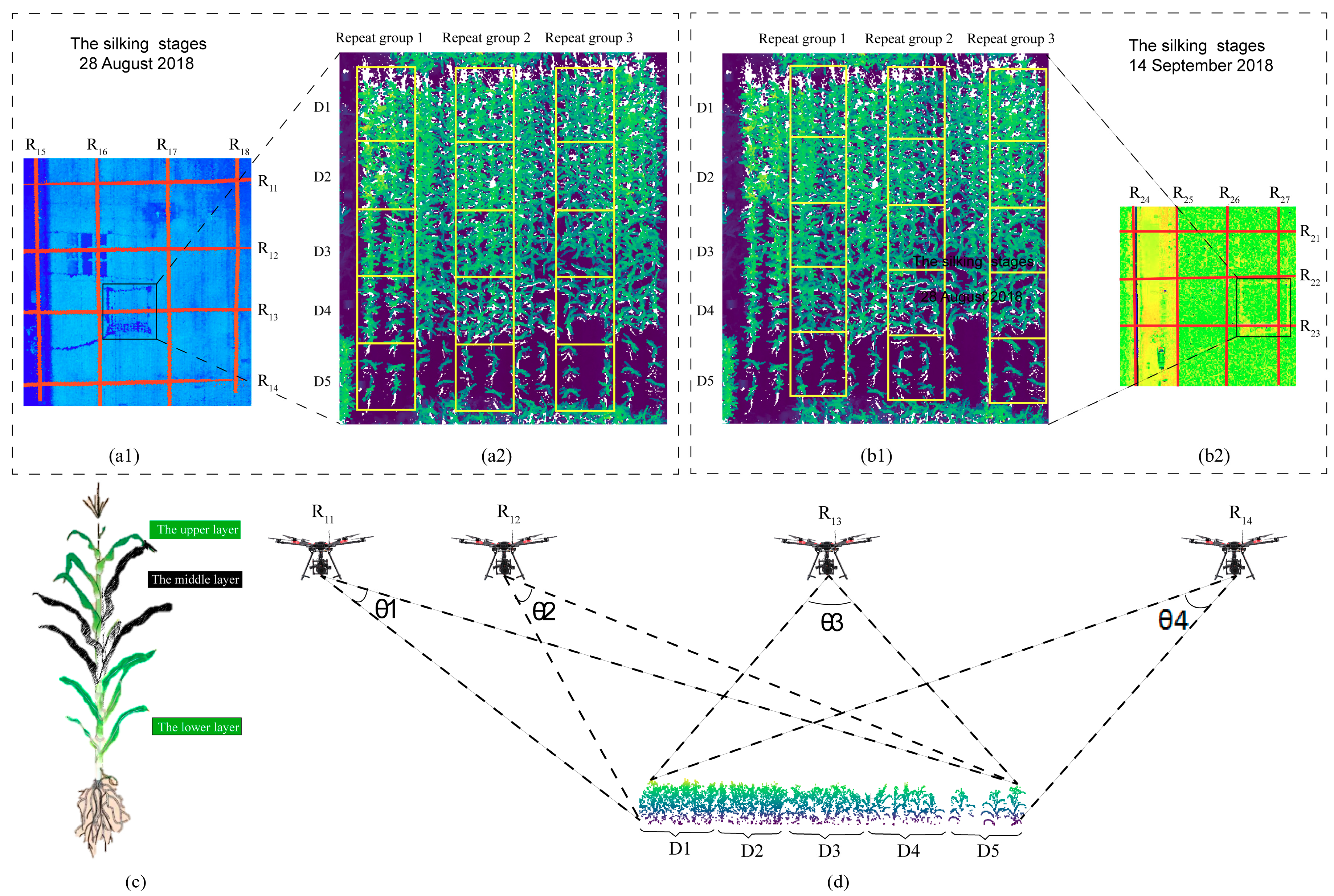
2.1. Experimental Design
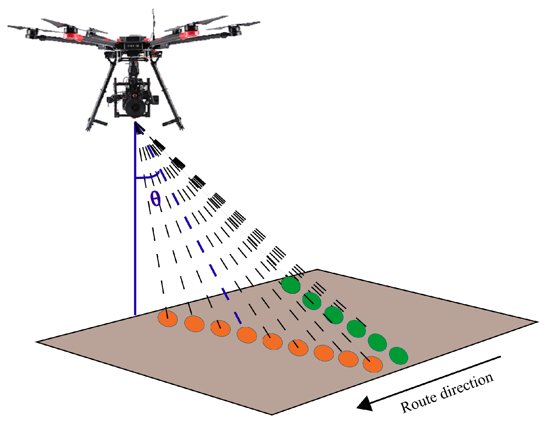
2.2. Data Acquisition
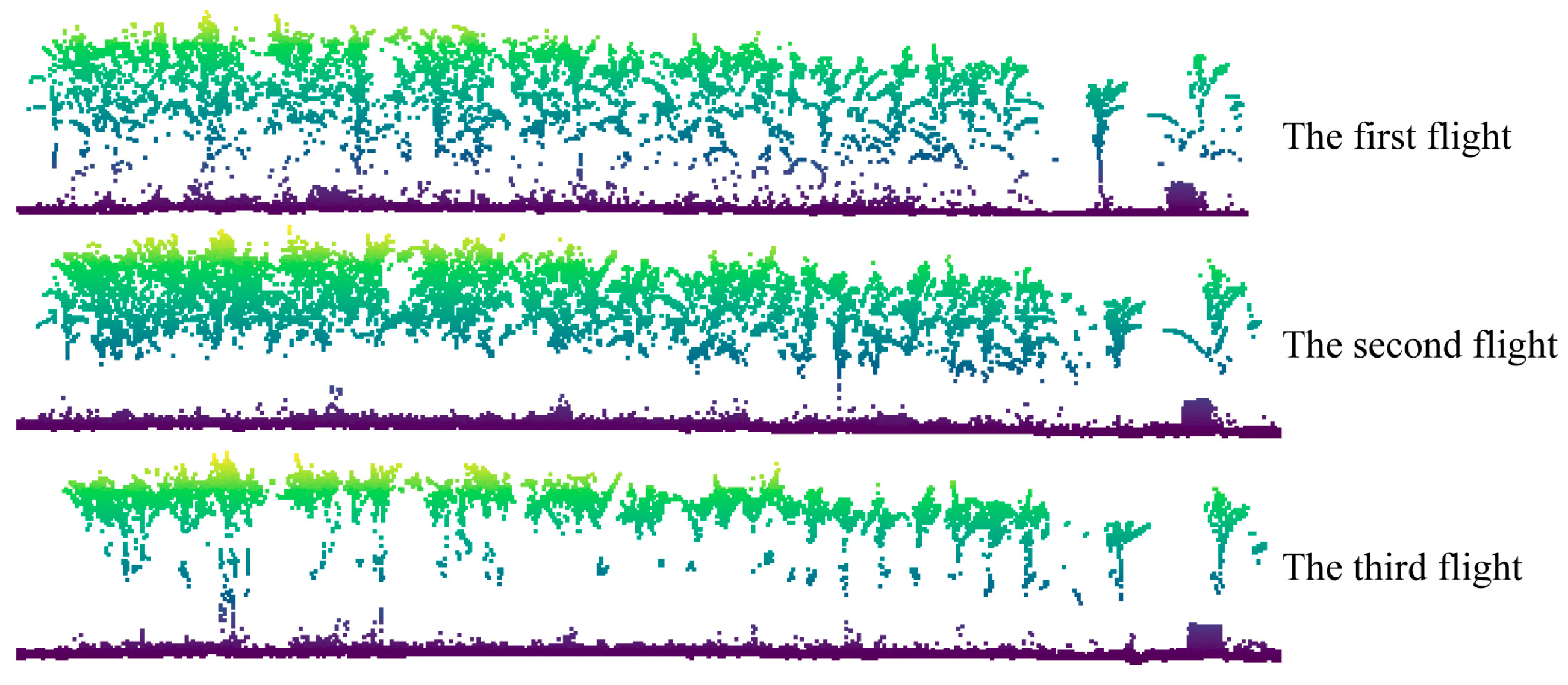
2.2.1. LiDAR Data
2.2.2. Field Data
2.3. Data Processing
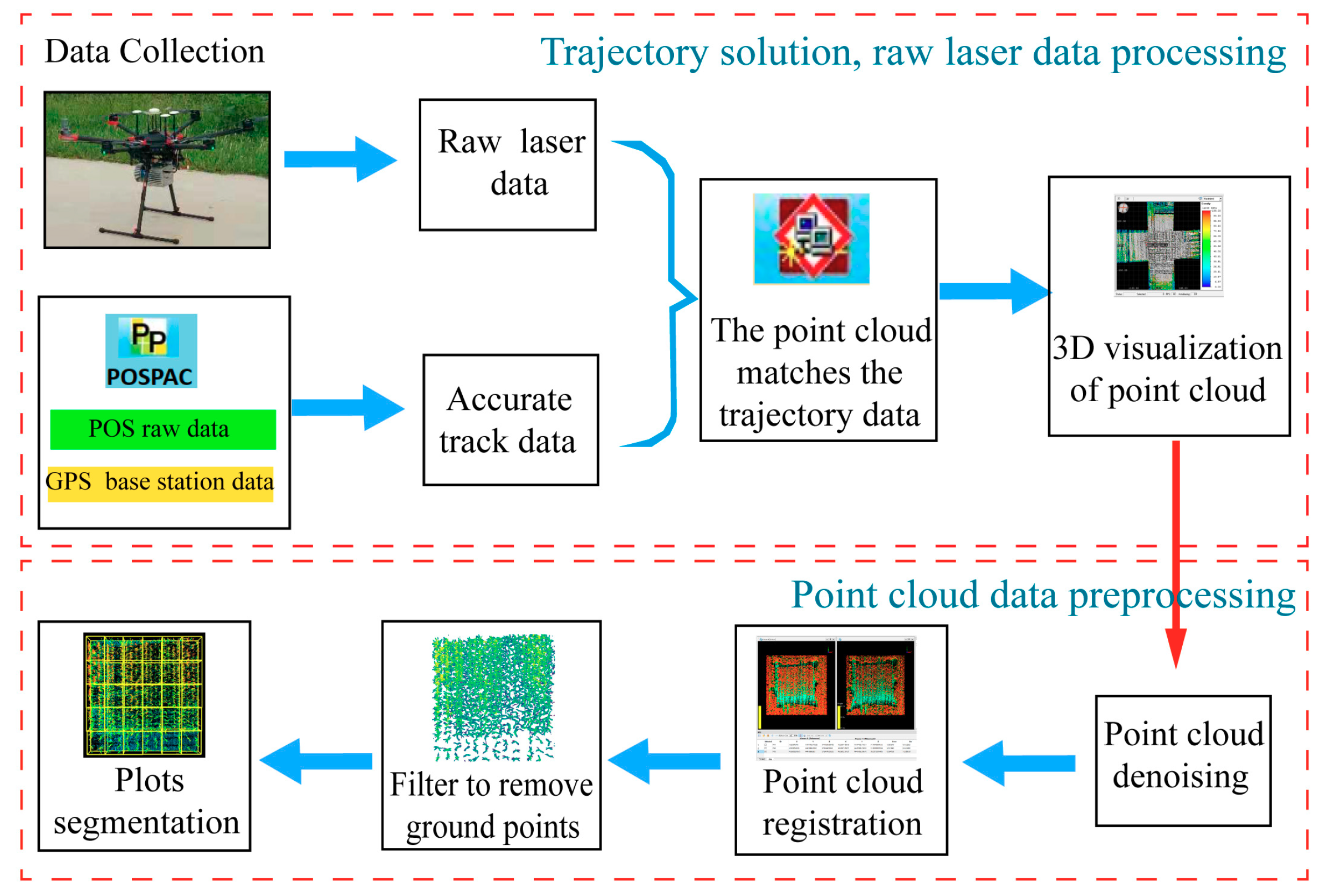
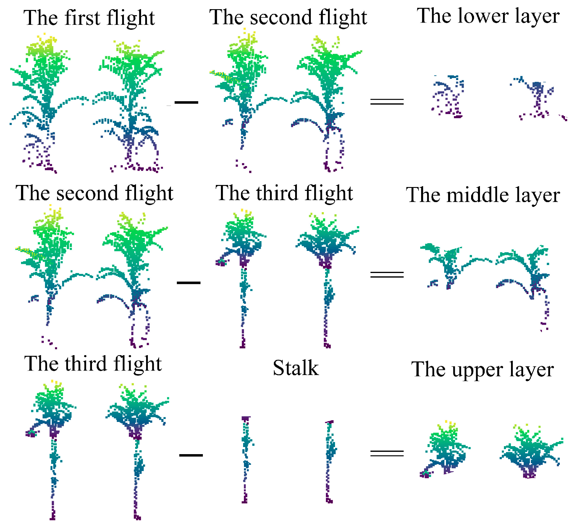
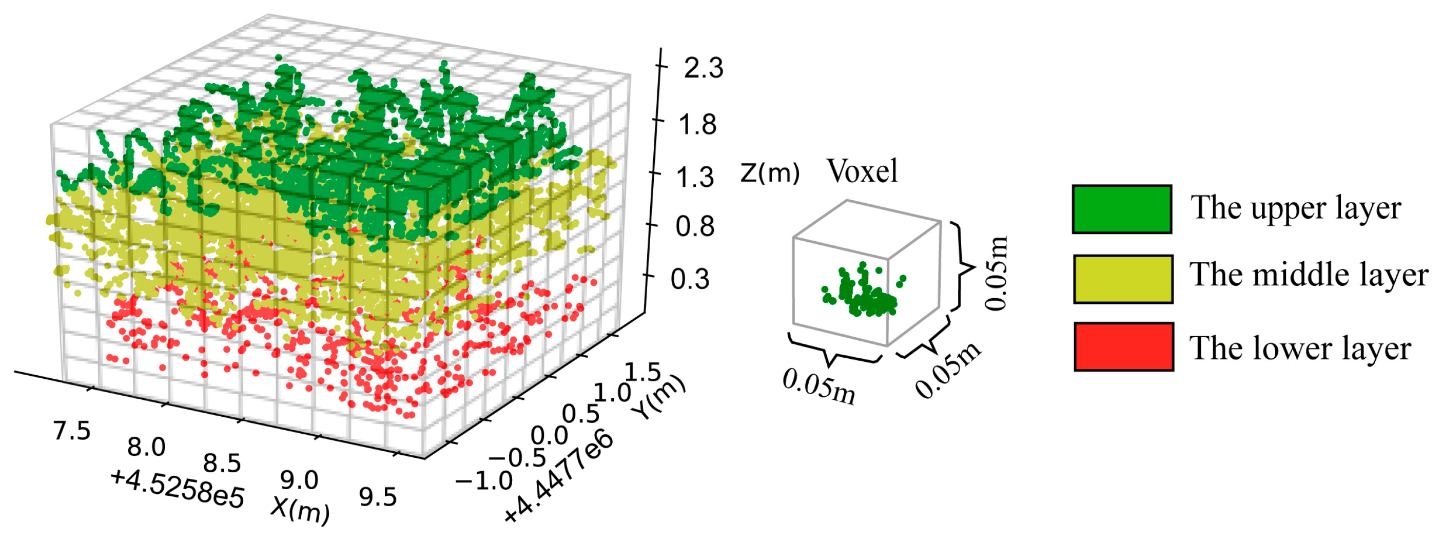
2.3.1. Data Preprocessing
2.3.2. Estimation of LAI
2.3.3. Analysis and Validation
3. Results
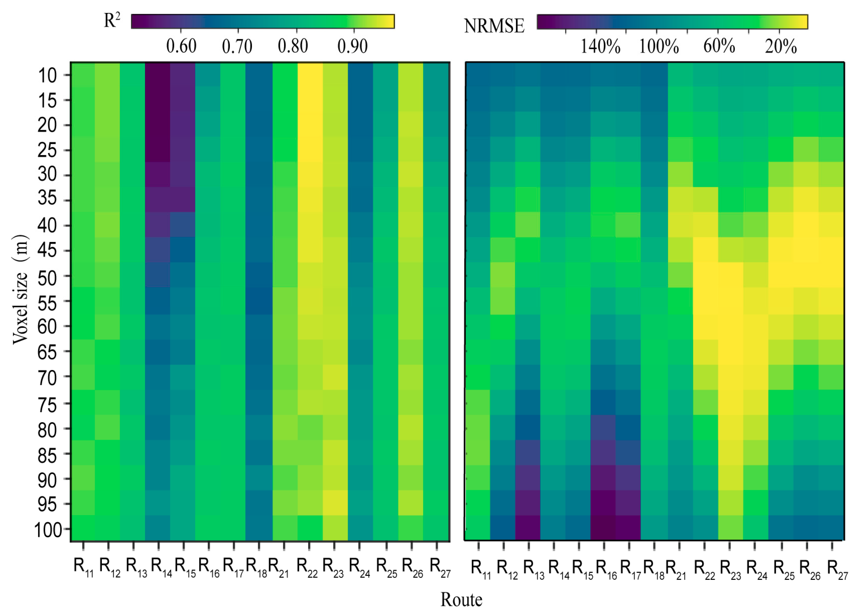
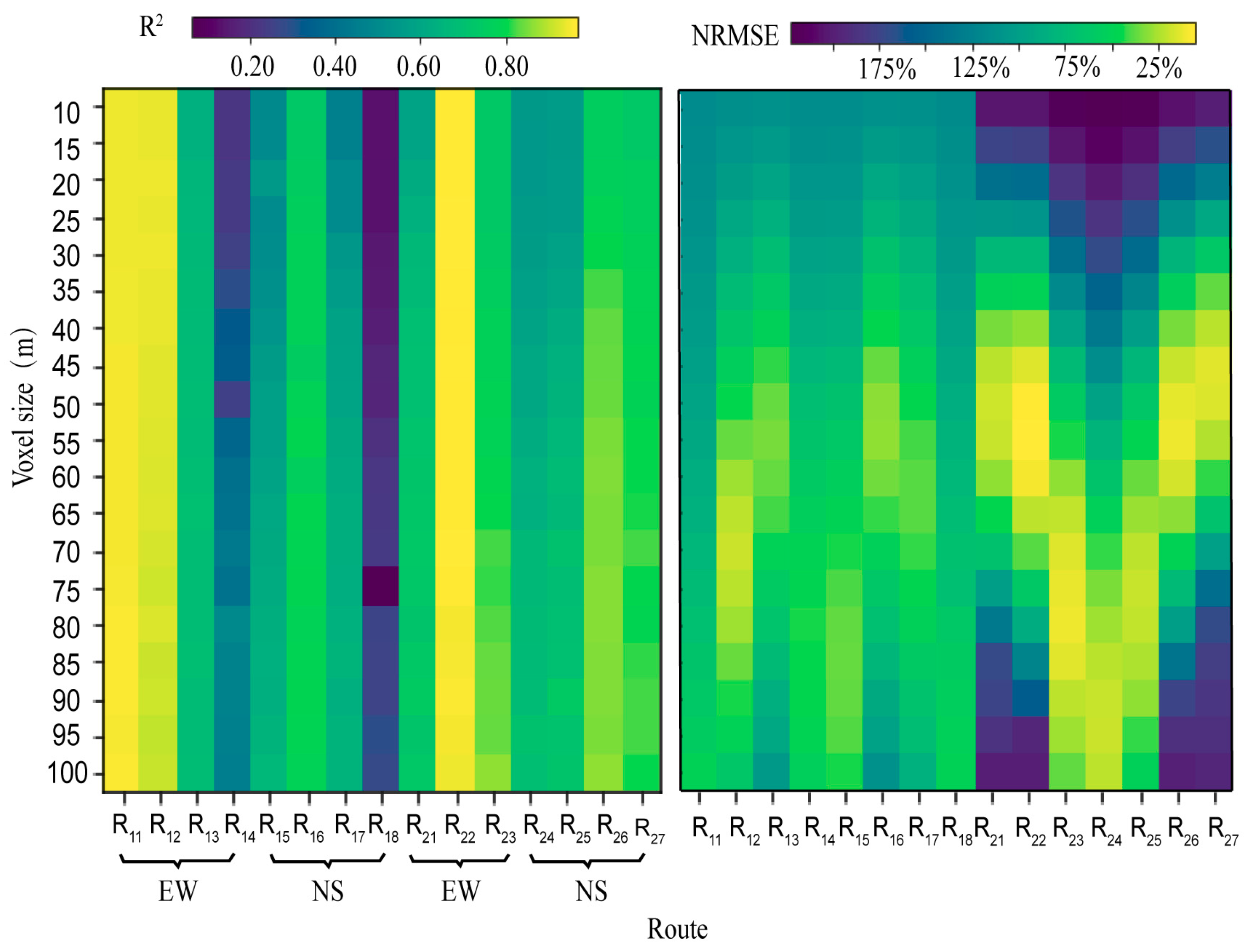
3.1. Determination of the Optimal Voxel Size
3.2. Relationship between Route Direction and Ridge Direction
3.3. Quantitative Analysis of the Occlusion Effect
4. Discussion
4.1. Analysis of the Optimal Incidence Angle
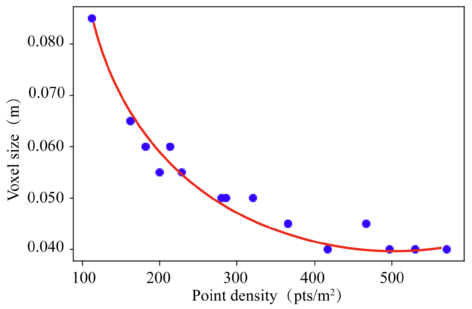
4.2. Factors Influencing the Selection of the Optimal Voxel Size
5. Conclusions
Author Contributions
Funding
Conflicts of Interest
References
- Hosseini, M.; McNairn, H.; Merzouki, A.; Pacheco, A. Estimation of Leaf Area Index (LAI) in corn and soybeans using multi-polarization C- and L-band radar data. Remote Sens. Environ. 2015, 170, 77–89. [Google Scholar] [CrossRef]
- CHEN, J.M.; BLACK, T.A. Defining leaf area index for non-flat leaves. Plant Cell Environ. 1992, 15, 421–429. [Google Scholar] [CrossRef]
- Chen, J.M.; Cihlar, J. Retrieving leaf area index of boreal conifer forests using Landsat TM images. Remote Sens. Environ. 1996, 55, 153–162. [Google Scholar] [CrossRef]
- Colombo, R. Retrieval of leaf area index in different vegetation types using high resolution satellite data. Remote Sens. Environ. 2003, 86, 120–131. [Google Scholar] [CrossRef]
- Yan, G.; Hu, R.; Luo, J.; Weiss, M.; Jiang, H.; Mu, X.; Xie, D.; Zhang, W. Review of indirect optical measurements of leaf area index: Recent advances, challenges, and perspectives. Agric. For. Meteorol. 2019, 265, 390–411. [Google Scholar] [CrossRef]
- Ryu, Y.; Sonnentag, O.; Nilson, T.; Vargas, R.; Kobayashi, H.; Wenk, R.; Baldocchi, D.D. How to quantify tree leaf area index in an open savanna ecosystem: A multi-instrument and multi-model approach. Agric. For. Meteorol. 2010, 150, 63–76. [Google Scholar] [CrossRef]
- Niu, Q.; Feng, H.; Yang, G.; Li, C.; Yang, H.; Xu, B.; Zhao, Y. Monitoring plant height and leaf area index of maize breeding material based on UAV digital images. Trans. Chin. Soc. Agric. Eng. 2018, 34, 73–82. [Google Scholar]
- Chen, J.M. Optically-based methods for measuring seasonal variation of leaf area index in boreal conifer stands. Agric. For. Meteorol. 1996, 80, 135–163. [Google Scholar] [CrossRef]
- Guo, Q.; Hu, T.; Liu, J. LiDAR Principles, Processing and Applications in Forest Ecology; Higher Education Press: Beijing, China, 2018; pp. 212–213. [Google Scholar]
- Lefsky, M.A.; Cohen, W.B.; Parker, G.G.; Harding, D.J. Lidar Remote Sensing for Ecosystem Studies. BioScience 2002, 52. [Google Scholar] [CrossRef]
- Cao, L.; Coops, N.C.; Innes, J.L.; Dai, J.; Ruan, H.; She, G. Tree species classification in subtropical forests using small-footprint full-waveform LiDAR data. Int. J. Appl. Earth Obs. Geoinf. 2016, 49, 39–51. [Google Scholar] [CrossRef]
- Hese, S.; Lucht, W.; Schmullius, C.; Barnsley, M.; Dubayah, R.; Knorr, D.; Neumann, K.; Riedel, T.; Schröter, K. Global biomass mapping for an improved understanding of the CO2 balance—The Earth observation mission Carbon-3D. Remote Sens. Environ. 2005, 94, 94–104. [Google Scholar] [CrossRef]
- Luo, S.; Wang, C.; Xi, X.; Pan, F. Estimating FPAR of maize canopy using airborne discrete-return LiDAR data. Opt. Express 2014, 22, 5106–5117. [Google Scholar] [CrossRef]
- Colaco, A.F.; Molin, J.P.; Rosell-Polo, J.R.; Escola, A. Application of light detection and ranging and ultrasonic sensors to high-throughput phenotyping and precision horticulture: Current status and challenges. Hortic. Res. 2018, 5, 35. [Google Scholar] [CrossRef]
- Malambo, L.; Popescu, S.C.; Murray, S.C.; Putman, E.; Pugh, N.A.; Horne, D.W.; Richardson, G.; Sheridan, R.; Rooney, W.L.; Avant, R.; et al. Multitemporal field-based plant height estimation using 3D point clouds generated from small unmanned aerial systems high-resolution imagery. Int. J. Appl. Earth Obs. Geoinf. 2018, 64, 31–42. [Google Scholar] [CrossRef]
- Jimenez-Berni, J.A.; Deery, D.M.; Rozas-Larraondo, P.; Condon, A.T.G.; Rebetzke, G.J.; James, R.A.; Bovill, W.D.; Furbank, R.T.; Sirault, X.R.R. High Throughput Determination of Plant Height, Ground Cover, and Above-Ground Biomass in Wheat with LiDAR. Front. Plant Sci. 2018, 9, 237. [Google Scholar] [CrossRef]
- Pang, Y.; Lefsky, M.; Sun, G.; Ranson, J. Impact of footprint diameter and off-nadir pointing on the precision of canopy height estimates from spaceborne lidar. Remote Sens. Environ. 2011, 115, 2798–2809. [Google Scholar] [CrossRef]
- Yang, W.; Ni-Meister, W.; Lee, S. Assessment of the impacts of surface topography, off-nadir pointing and vegetation structure on vegetation lidar waveforms using an extended geometric optical and radiative transfer model. Remote Sens. Environ. 2011, 115, 2810–2822. [Google Scholar] [CrossRef]
- Chen, Y.; Zhang, W.; Hu, R.; Qi, J.; Shao, J.; Li, D.; Wan, P.; Qiao, C.; Shen, A.; Yan, G. Estimation of forest leaf area index using terrestrial laser scanning data and path length distribution model in open-canopy forests. Agric. For. Meteorol. 2018, 263, 323–333. [Google Scholar] [CrossRef]
- Zhu, X.; Skidmore, A.K.; Wang, T.; Liu, J.; Darvishzadeh, R.; Shi, Y.; Premier, J.; Heurich, M. Improving leaf area index (LAI) estimation by correcting for clumping and woody effects using terrestrial laser scanning. Agric. For. Meteorol. 2018, 263, 276–286. [Google Scholar] [CrossRef]
- Hu, R.; Yan, G.; Mu, X.; Luo, J. Indirect measurement of leaf area index on the basis of path length distribution. Remote Sens. Environ. 2014, 155, 239–247. [Google Scholar] [CrossRef]
- Su, W.; Zhu, D.; Huang, J.; Guo, H. Estimation of the vertical leaf area profile of corn (Zea mays) plants using terrestrial laser scanning (TLS). Comput. Electr. Agric. 2018, 150, 5–13. [Google Scholar] [CrossRef]
- Zhang, Z.; Cao, L.; She, G. Estimating Forest Structural Parameters Using Canopy Metrics Derived from Airborne LiDAR Data in Subtropical Forests. Remote Sens. 2017, 9, 940. [Google Scholar] [CrossRef]
- Holmgren, J.; Nilsson, M.; Olsson, H. Simulating the effects of lidar scanning angle for estimation of mean tree height and canopy closure. Can. J. Remote Sens. 2003, 29, 623–632. [Google Scholar] [CrossRef]
- Bauwens, S.; Bartholomeus, H.; Calders, K.; Lejeune, P. Forest Inventory with Terrestrial LiDAR: A Comparison of Static and Hand-Held Mobile Laser Scanning. Forests 2016, 7, 127. [Google Scholar] [CrossRef]
- Hamraz, H.; Contreras, M.A.; Zhang, J. Forest understory trees can be segmented accurately within sufficiently dense airborne laser scanning point clouds. Sci. Rep. 2017, 7, 6770. [Google Scholar] [CrossRef] [Green Version]
- Su, Y.; Wu, F.; Ao, Z.; Jin, S.; Qin, F.; Liu, B.; Pang, S.; Liu, L.; Guo, Q. Evaluating maize phenotype dynamics under drought stress using terrestrial lidar. Plant Methods 2019, 15. [Google Scholar] [CrossRef]
- Qin, H.; Wang, C.; Pan, F.; Lin, Y.; Xi, X.; Luo, S. Estimation of FPAR and FPAR profile for maize canopies using airborne LiDAR. Ecol. Indic. 2017, 83, 53–61. [Google Scholar] [CrossRef]
- Liu, L.; Pang, Y.; Li, Z.; Si, L.; Liao, S. Combining Airborne and Terrestrial Laser Scanning Technologies to Measure Forest Understorey Volume. Forests 2017, 8, 111. [Google Scholar] [CrossRef]
- Hilker, T.; van Leeuwen, M.; Coops, N.C.; Wulder, M.A.; Newnham, G.J.; Jupp, D.L.B.; Culvenor, D.S. Comparing canopy metrics derived from terrestrial and airborne laser scanning in a Douglas-fir dominated forest stand. Trees 2010, 24, 819–832. [Google Scholar] [CrossRef]
- Song, X.; Yang, G.; Yang, C.; Wang, J.; Cui, B. Spatial Variability Analysis of Within-Field Winter Wheat Nitrogen and Grain Quality Using Canopy Fluorescence Sensor Measurements. Remote Sens. 2017, 9, 237. [Google Scholar] [CrossRef]
- Ritchie, S.W.; Hanway, J.J.; Benson, G.O. How a Corn Plant Develops; Iowa State University: Ames, Iowa, 1993. [Google Scholar]
- Hosoi, F.; Omasa, K. Voxel-Based 3-D Modeling of Individual Trees for Estimating Leaf Area Density Using High-Resolution Portable Scanning Lidar. IEEE Trans. Geosci. Remote Sens. 2006, 44, 3610–3618. [Google Scholar] [CrossRef]
- Yao, Y.; Fan, W.; Liu, Q.; Li, L.; Tao, X.; Xin, X.; Liu, Q. Improved harvesting method for corn LAI measurement in corn whole growth stages. Trans. Chin. Soc. Agric. Eng. 2010, 26, 189–194. [Google Scholar]
- Zheng, G.; Moskal, L.M. Computational-Geometry-Based Retrieval of Effective Leaf Area Index Using Terrestrial Laser Scanning. IEEE Trans. Geosci. Remote Sens. 2012, 50, 3958–3969. [Google Scholar] [CrossRef]
- Korhonen, L.; Korpela, I.; Heiskanen, J.; Maltamo, M. Airborne discrete-return LIDAR data in the estimation of vertical canopy cover, angular canopy closure and leaf area index. Remote Sens. Environ. 2011, 115, 1065–1080. [Google Scholar] [CrossRef]
- Liu, J.; Skidmore, A.K.; Jones, S.; Wang, T.; Heurich, M.; Zhu, X.; Shi, Y. Large off-nadir scan angle of airborne LiDAR can severely affect the estimates of forest structure metrics. ISPRS J. Photogramm. Remote Sens. 2018, 136, 13–25. [Google Scholar] [CrossRef]
- Oshio, H.; Asawa, T.; Hoyano, A.; Miyasaka, S. Estimation of the leaf area density distribution of individual trees using high-resolution and multi-return airborne LiDAR data. Remote Sens. Environ. 2015, 166, 116–125. [Google Scholar] [CrossRef]
- Béland, M.; Widlowski, J.-L.; Fournier, R.A. A model for deriving voxel-level tree leaf area density estimates from ground-based LiDAR. Environ. Model. Softw. 2014, 51, 184–189. [Google Scholar] [CrossRef]
- Li, J.; Hu, B.; Noland, T.L. Classification of tree species based on structural features derived from high density LiDAR data. Agric. For. Meteorol. 2013, 171–172, 104–114. [Google Scholar] [CrossRef]
- Grau, E.; Durrieu, S.; Fournier, R.; Gastellu-Etchegorry, J.-P.; Yin, T. Estimation of 3D vegetation density with Terrestrial Laser Scanning data using voxels. A sensitivity analysis of influencing parameters. Remote Sens. Environ. 2017, 191, 373–388. [Google Scholar] [CrossRef]


| Direction | Route | Angle (°) | Point Cloud Density (pts/m2) |
|---|---|---|---|
| EW | R11 | 69 to 77 | 112 |
| R12 | −64 to −32 | 280 | |
| R13 | −34 to 29 | 529 | |
| R14 | 60 to 74 | 213 | |
| NS | R15 | 63 to 73 | 228 |
| R16 | −54 to 0 | 496 | |
| R17 | −60 to −25 | 417 | |
| R18 | 68 to 76 | 162 | |
| EW | R21 | −14 to 3 | 570 |
| R22 | −12 to −5 | 285 | |
| R23 | 8 to 32 | 200 | |
| NS | R24 | 11 to 64 | 182 |
| R25 | −30 to 0 | 321 | |
| R26 | 3 to 18 | 466 | |
| R27 | −2 to 7 | 366 |
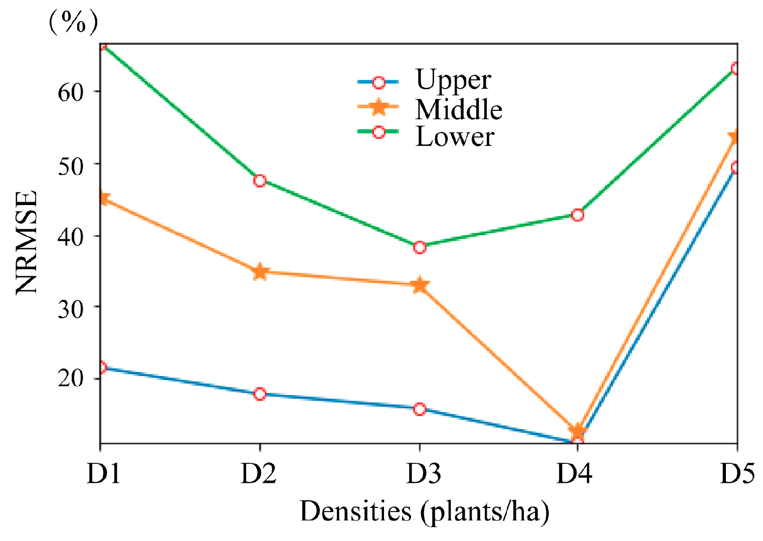
| Layers | Densities | Mean | Maximum | Minimum | CV (%) |
|---|---|---|---|---|---|
| Upper | D1 | 1.07 | 1.55 | 0.84 | 6.36 |
| D2 | 0.73 | 0.85 | 0.48 | 2.54 | |
| D3 | 0.59 | 0.72 | 0.47 | 1.59 | |
| D4 | 0.38 | 0.47 | 0.23 | 1.85 | |
| D5 | 0.10 | 0.14 | 0.06 | 0.77 | |
| Middle | D1 | 1.39 | 1.87 | 1.07 | 6.49 |
| D2 | 1.15 | 1.29 | 0.98 | 1.16 | |
| D3 | 0.92 | 1.04 | 0.83 | 0.92 | |
| D4 | 0.56 | 0.77 | 0.37 | 3.78 | |
| D5 | 0.14 | 0.17 | 0.09 | 0.53 | |
| Lower | D1 | 0.55 | 0.98 | 0.20 | 17.63 |
| D2 | 0.49 | 0.87 | 0.25 | 13.73 | |
| D3 | 0.38 | 0.57 | 0.30 | 3.01 | |
| D4 | 0.22 | 0.39 | 0.14 | 3.76 | |
| D5 | 0.06 | 0.09 | 0.04 | 0.44 |
| Routes | NRMSE (%) | R2 | Optimal Voxel Size (m) |
|---|---|---|---|
| R11 | 27.0 | 0.85 | 0.085 |
| R12 | 24.5 | 0.90 | 0.050 |
| R13 | 28.6 | 0.85 | 0.040 |
| R14 | 43.7 | 0.69 | 0.060 |
| R15 | 39.6 | 0.70 | 0.055 |
| R16 | 33.3 | 0.82 | 0.040 |
| R17 | 30.3 | 0.85 | 0.040 |
| R18 | 42.7 | 0.67 | 0.065 |
| R21 | 11.2 | 0.90 | 0.040 |
| R22 | 1.9 | 0.94 | 0.050 |
| R23 | 3.2 | 0.92 | 0.055 |
| R24 | 5.8 | 0.74 | 0.060 |
| R25 | 3.6 | 0.84 | 0.050 |
| R26 | 1.9 | 0.93 | 0.045 |
| R27 | 3.4 | 0.83 | 0.045 |
| Direction | Routes | Angle (°) | NRMSE (%) | R2 |
|---|---|---|---|---|
| EW | R11 | 69–77 | 63.6 | 0.96 |
| R12 | −64–−32 | 42.5 | 0.93 | |
| R13 | −34–29 | 49.3 | 0.68 | |
| R14 | 60–74 | 57.3 | 0.40 | |
| R22 | −12–−5 | 4.6 | 0.96 | |
| R23 | 8–32 | 41.0 | 0.78 | |
| NS | R15 | 63–73 | 59.3 | 0.58 |
| R16 | −54–0 | 43.8 | 0.77 | |
| R17 | −60–−25 | 59.7 | 0.58 | |
| R18 | 68–76 | 71.1 | 0.23 | |
| R26 | 3–18 | 17.7 | 0.84 | |
| R25 | −30–0 | 60.5 | 0.65 |
| Incidence Angle Classification | Route | Angle (°) | NRMSE (%) | R2 |
|---|---|---|---|---|
| Angle 1 | R11 | 69 to 77 | 63.6 | 0.96 |
| R14 | 60 to 74 | 57.3 | 0.40 | |
| R15 | 60 to 73 | 59.3 | 0.58 | |
| R18 | 68 to 76 | 71.7 | 0.23 | |
| Angle 2 | R13 | −34 to 29 | 49.3 | 0.68 |
| R16 | −54 to 0 | 43.8 | 0.77 | |
| R25 | −30 to 0 | 60.5 | 0.84 | |
| Angle 3 | R24 | 11 to 64 | 63.1 | 0.64 |
| R12 | −64 to −32 | 42.5 | 0.93 | |
| R17 | −60 to −25 | 59.7 | 0.58 | |
| R23 | 8 to 32 | 41.0 | 0.78 | |
| Angle 4 | R21 | −14 to 3 | 31.6 | 0.69 |
| R27 | −2 to 7 | 11.7 | 0.79 | |
| Angle 5 | R26 | 3 to 18 | 17.7 | 0.84 |
| R22 | −12 to −5 | 4.6 | 0.96 |
© 2019 by the authors. Licensee MDPI, Basel, Switzerland. This article is an open access article distributed under the terms and conditions of the Creative Commons Attribution (CC BY) license (http://creativecommons.org/licenses/by/4.0/).
Share and Cite
Lei, L.; Qiu, C.; Li, Z.; Han, D.; Han, L.; Zhu, Y.; Wu, J.; Xu, B.; Feng, H.; Yang, H.; et al. Effect of Leaf Occlusion on Leaf Area Index Inversion of Maize Using UAV–LiDAR Data. Remote Sens. 2019, 11, 1067. https://0-doi-org.brum.beds.ac.uk/10.3390/rs11091067
Lei L, Qiu C, Li Z, Han D, Han L, Zhu Y, Wu J, Xu B, Feng H, Yang H, et al. Effect of Leaf Occlusion on Leaf Area Index Inversion of Maize Using UAV–LiDAR Data. Remote Sensing. 2019; 11(9):1067. https://0-doi-org.brum.beds.ac.uk/10.3390/rs11091067
Chicago/Turabian StyleLei, Lei, Chunxia Qiu, Zhenhai Li, Dong Han, Liang Han, Yaohui Zhu, Jintao Wu, Bo Xu, Haikuan Feng, Hao Yang, and et al. 2019. "Effect of Leaf Occlusion on Leaf Area Index Inversion of Maize Using UAV–LiDAR Data" Remote Sensing 11, no. 9: 1067. https://0-doi-org.brum.beds.ac.uk/10.3390/rs11091067