Impacts of Climate Change on Lake Fluctuations in the Hindu Kush-Himalaya-Tibetan Plateau


1
School of Geographical Sciences, Guangzhou University, Guangzhou 510006, China
2
Rural Non-Point Source Pollution Comprehensive Management Technology Center of Guangdong Province, Guangzhou University, Guangzhou 510006, China
3
Department of Geography, National University of Singapore, Singapore 117570, Singapore
4
Inner Mongolia Key Lab of River and Lake Ecology, Inner Mongolia University, Hohhot 010021, China
5
Earth Observatory of Singapore, Nanyang Technological University, Singapore 639798, Singapore
6
Department of Land, Environment, Agriculture and Forestry, University of Padova, Agripolis, viale dell’Università 16, 35020 Legnaro (PD), Italy
*
Author to whom correspondence should be addressed.
Remote Sens. 2019, 11(9), 1082; https://0-doi-org.brum.beds.ac.uk/10.3390/rs11091082
Submission received: 22 March 2019
/
Revised: 29 April 2019
/
Accepted: 4 May 2019
/
Published: 7 May 2019
(This article belongs to the Special Issue Remote Sensing of Large Rivers)
Abstract
:Lakes in the Hindu Kush-Himalaya-Tibetan (HKHT) regions are crucial indicators for the combined impacts of regional climate change and resultant glacier retreat. However, they lack long-term systematic monitoring and thus their responses to recent climatic change still remain only partially understood. This study investigated lake extent fluctuations in the HKHT regions over the past 40 years using Landsat (MSS/TM/ETM+/OLI) images obtained from the 1970s to 2014. Influenced by different regional atmospheric circulation systems, our results show that lake changing patterns are distinct from region to region, with the most intensive lake shrinking observed in northeastern HKHT (HKHT Interior, Tarim, Yellow, Yangtze), while the most extensive expansion was observed in the western and southwestern HKHT (Amu Darya, Ganges Indus and Brahmaputra), largely caused by the proliferation of small lakes in high-altitude regions during 1970s–1995. In the past 20 years, extensive lake expansions (~39.6% in area and ~119.1% in quantity) were observed in all HKHT regions. Climate change, especially precipitation change, is the major driving force to the changing dynamics of the lake fluctuations; however, effects from the glacier melting were also significant, which contributed approximately 31.9–40.5%, 16.5–39.3%, 12.8–29.0%, and 3.3–6.1% of runoff to lakes in the headwaters of the Tarim, Amu Darya, Indus, and Ganges, respectively. We consider that the findings in this paper could have both immediate and long-term implications for dealing with water-related hazards, controlling glacial lake outburst floods, and securing water resources in the HKHT regions, which contain the headwater sources for some of the largest rivers in Asia that sustain 1.3 billion people.
1. Introduction
The Earth’s climate is changing due to human emissions of greenhouse gases and is projected to continuously change throughout the 21st century, even at unprecedented rates in recent human history [1]. Impacts of climate change on high-elevation regions (e.g., the Himalayas, Rockies, Andes, and the Alps) are expected to be much more significant due to their higher sensitivity to temperature and precipitation changes [2]. Therefore, lakes in the high-elevation regions have been considered one of the most efficient indicators of terrestrial climate change [3,4]; however, investigating their responses to the combined impacts of both climate change and resultant glacier retreat still remains largely unknown.
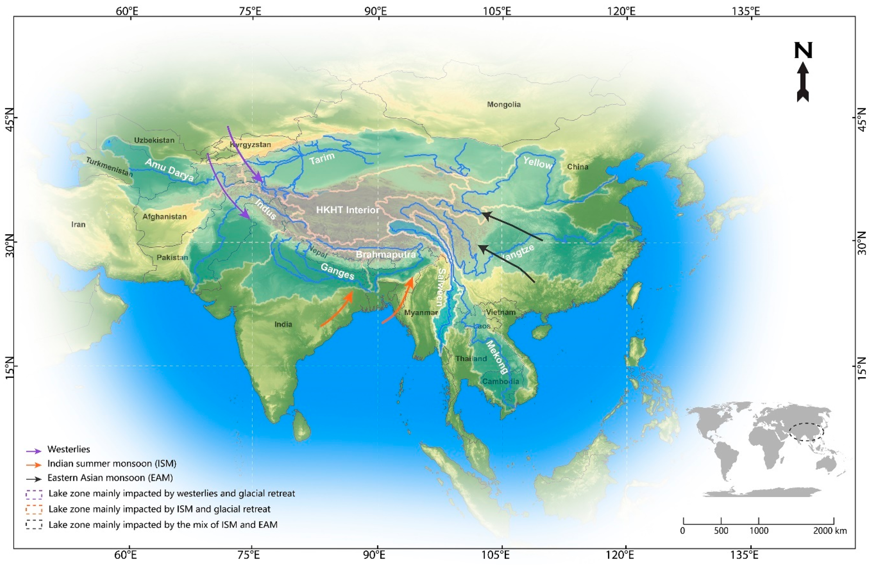
The Hindu Kush-Himalaya-Tibetan (HKHT) regions, with a total lake surface area over 50,000 km2, are the highest lake regions on Earth. The lakes in these regions play important roles in maintaining the water balance of some of the largest Asian rivers [5,6] (Figure 1), and for hydrological cycles that sustain around 1.3 billion people in Asia [7]. Over the past decades, the HKHT regions have experienced dramatic climate changes [8]. The most widely reported effects include rapid alterations of hydrological cycles that were caused simultaneously by climate change and its induced-glacier retreat. These will undoubtedly cause disruptions to downstream water supplies [2,9,10]. Ongoing climate change over succeeding decades could have additional negative impacts across these regions, including cascading effects on downstream river flows, water-related hazards, glacial lake outburst floods, and on riverine biodiversity [11,12]. Lake systems in this area are key components within the hydrological cycles largely controlling the supply and storage of water. However, they have recently experienced strong spatiotemporally heterogeneous changes in their hydrological regimes [13,14,15]. As most lakes in this region are rarely impacted by anthropogenic activities [16], it is of a paramount importance to investigate the coupled impacts of climate change and glacier retreat on hydrological cycles and other related environmental disturbances in the HKHT regions.
The increasing availability of satellite remote sensing data with sufficient spatiotemporal resolutions and their global coverage allow for rapid and cost-effective investigations of lake fluctuations across large areas over a longer-term. Applications of remote sensing are thus advantageous over traditional field-based methods in detecting and analyzing the dynamics of alpine lakes, such as changes in lake abundance, surface elevation, water storage, surface area, and their interactions with glaciers. Such approaches are even more beneficial in studying lakes in remote areas like HKHT regions where field-based lake measurements are limited. There are several studies that have investigated lake changes using satellite imagery in the HKHT regions: Gardelle, Arnaud [17], Khadka, Zhang [18], Kulkarni, Rathore [19], Lei, Yang [14], Mao, Wang [20], Mergili, Müller [21], Song, Huang [13], Yang and Lu [22], Zhang, Yao [23], and Zhou, Wang [15]. These studies used a few representative years (i.e., 1975, 1990, and 2000) to examine the lake responses to climate change. However, a continuous lake fluctuation history at annual-resolution has not yet been analyzed; and furthermore, the role of glacier retreat in lake fluctuation history has never been examined before.
Here we investigated lake extent fluctuation history and its relationship with climate change and glacier retreat in the entire HKHT regions (e.g., the upstream regions of the Amu Darya, Indus, Ganges, Brahmaputra, Salween, Mekong, Yangtze, Yellow and Tarim rivers, plus the HKHT Interior) over the past 40 years mainly using remote sensing techniques. We analyzed 3910 Landsat-MSS/TM/ETM+/OLI images (Figure 2) on the Google Earth Engine Platform using supervised classification. Using the lake surface area delineated annually (A) and estimated water storage volume (S), we derived inter-annual lake water storage change (ΔS), which indicates the lake water balance changes. This balance is the result of lake inflow, precipitation, and evaporation over the lake water area [13,15]. Since precipitation and evaporation over the lake water area could be driven from climatic data, the annual river inflow and runoff could be calculated. Based on this principle, a catchment water balance model was developed to assess the lake runoff composition, which was then used to identify the predominant driving forces to lake fluctuations over the past 40 years in this area. The objective of this study is to address the following questions: (1) How did the lakes in the HKHT regions respond to climate change and glacier retreat? (2) What are the patterns of lake fluctuation in different regions and what are the driving forces of these? (3) What is the role of glacier retreat in lake fluctuation history?
2. Datasets and Methods
2.1. Datasets and Data Processing
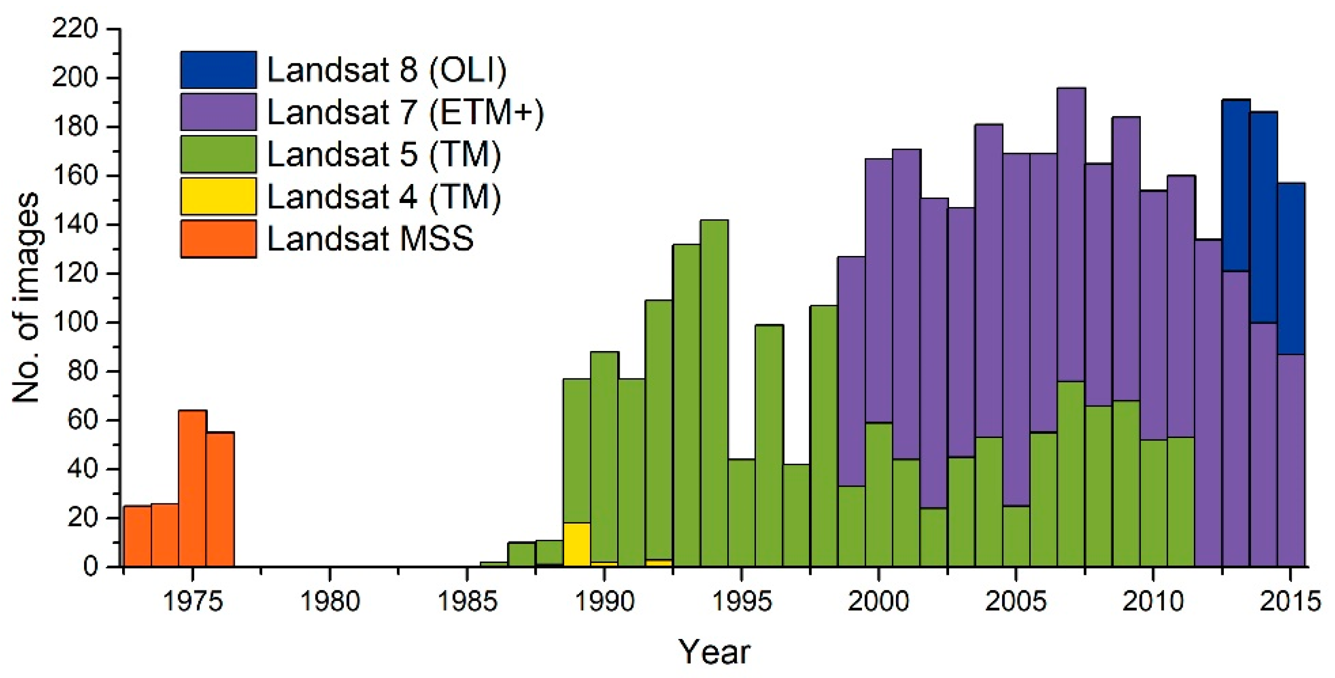
The study area covered all the HKHT regions and the HKHT Interior, a total of 3.85 million km2, which is equivalent to the 4.28 billion Landsat pixels (30 m). Initial water detection was performed using Google Earth Engine (GEE), a free cloud platform with large-scale computational facility designed for parallel computation of satellite imagery. GEE includes an almost complete image set of Landsat MSS (60 m)/TM (30 m)/ETM+ (30 m)/OLI (30 m) obtained from the USGS Earth Resources Observation and Science archive. We selected 3910 dry-season (from September to November) images from a total of 9124 available Landsat images (Figure 2). Dry-season images are useful in lake delineation as they generally represent the annual hydrological condition. Satellite images were pre-processed with standard procedures including: (1) image resampling to ensure all images have consistent spatial resolution of 30 m, (2) transformation of raw digital numbers to top of atmosphere reflectance based on image metadata using a method developed by NASA [24], and (3) cloud removal. All preprocessing procedures were checked covering all the major river basins in the HKHT regions based on an approach prototyped for the Tibetan Plateau.
To analyze the causes of lake fluctuations, some other auxiliary datasets (other than Landsats) were used, which are summarized in Table 1. These datasets can be divided into four categories: (1) grid-interpolated climatic data based on ground observations, including daily mean temperature, precipitation, evapotranspiration, solar radiation, soil moisture, and derived monthly and yearly products; (2) yearly land cover data, which are secondary products derived from Landsat images during lake delineation using supervised image classification techniques; (3) geomorphic data derived from grid DEM data; and (4) some ancillary data, such as glacier spatial distribution, reliable information about lake surface area, and storage volume. The ancillary data, used to validate and enhance our results, were collected from various sources, such as official reports from governments, public lake databases (e.g., World Lake Database (http://wldb.ilec.or.jp/), Global Lake Database (http://www.worldlakes.org/lakes.asp), China Lake Scientific Database and Chinese lake catalogs), as well as results released by previous studies [22,25,26]. We were very conservative in data collection; i.e., only lake storage volumes that appeared in multiple sources were used to guarantee the data quality. After preprocessing, all raster data were co-registered, correlated, organized by year, merged as an annual product, and converted to Tagged Image File Format (TIFF) files. This chain of processing was performed using Python programming with integrated ArcGIS ArcPy scripting module to generate batch processing tasks to handle large image datasets.
2.2. Lake Delineation
We delineated lakes by analyzing 3910 Landsat images on the GEE platform using a supervised classification method by a support vector machine (SVM) classifier [32]. 400 regions of interest (ROI) for six classes (snow and glacier, bare land, meadowland, forest land, water body, and cropland) were visually digitized from Google Earth high-resolution images from different years to assess the spectral characteristics and to assign a class to each image pixel according to mathematical algorithms [33]. SVMs are an attractive option in water body investigations due to their capability to generalize well with limited training samples (i.e., a common limitation for remote sensing of remote places like the HKHT region). The SVM methods classify objects through the concept of the margin, which is defined to be the shortest distance between the decision boundary and any of the samples. The decision boundary is chosen to be the one for which the margin is maximized. The margin is defined as the perpendicular distance between the decision boundary and the closest of the data points. Maximizing the margin leads to a particular choice of decision boundary. The location of this boundary is determined by a subset of the data points, known as support vectors [34]. The overall accuracy was accessed using confusion matrices, based on another 1000 ROIs. However, the major concern for this study was water bodies. The deviation area index (DAI) [22,35] was used to quantify the difference between the lake surface area derived from Landsat images and the area delineated using high-resolution images from Google Earth in the same year. The DAI is defined as follows:
where is the surface area of lakes and reservoirs delineated in high resolution images using Google Earth polygon tool; is the surface area derived from Landsat images. The DAI values generally vary from −∞ to 1. Water bodies with values close to zero have the best match between the two areas, while moving to the extremes indicate higher deviations. 200 randomly selected lakes with an area range of 0.1 km2—484 km2 were tested and validated using this index.
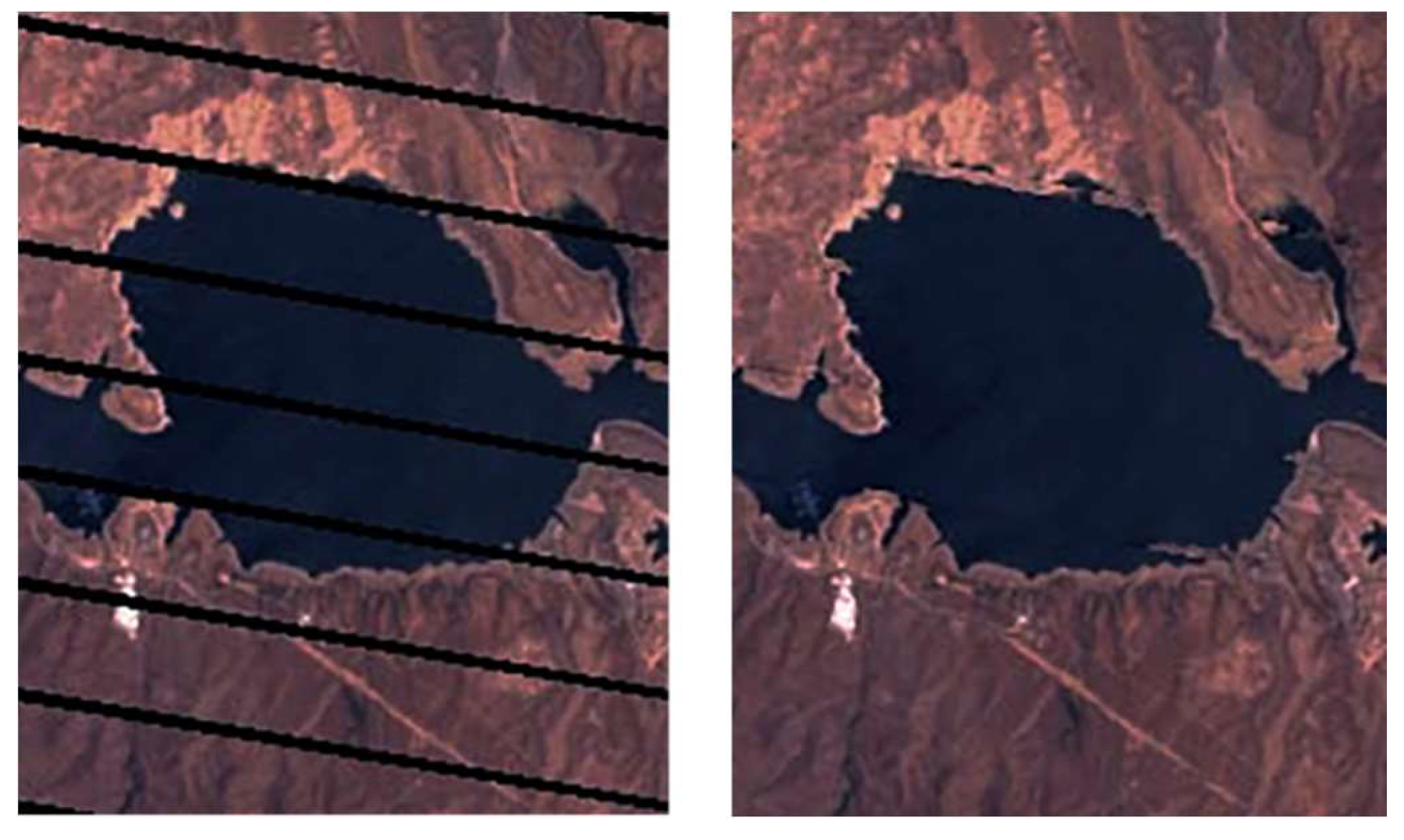
We carried out supervised classification of 170 Landsat MSS images to obtain the initial look of the lake status and quantity in the 1970s. The MSS images were primarily obtained from the image collection of Landsat Global Land Survey 1975. However, because of the failure of the Landsat 4, no complete annual results were produced for the years 1976–1988. The subsequent data for the year 1989 was primarily produced from Landsat-4 and -5 imageries. A few gaps were filled with scenes acquired by Landsat MSS images. The data was then updated using 2323 Landsat TM/ETM+/OLI images on a year-by-year basis. Yearly products for 1989 to 2014 were derived. In 2003, the scan-line corrector (SLC) on the Landsat ETM+ failed, and the images acquired after the SLC failure are referred to as SLC-off images. SLC gap-filled products phase one methodology [36] was used to fill the gaps in Landsat SLC-off images to be used in this study. Gap filling first requires you to identify the location within an image to be filled. A gap mask was established for each band that marks existing data with 1 and missing data in the gap and fill areas with 0. These gap masks could be directly obtained from GEE. The masks were provided in 8-bit images with identical dimensions to the corresponding image bands. Once the gaps are identified, the linear histogram matching approach was used to find a linear transformation between one product to another, which was used to fill the gaps with previously acquired Landsat ETM+ images (Figure 3).
After classification, water bodies were co-registered, correlated, organized by year, and then were converted to polygons stored in a geodatabase. For small polygons with an area lower than 0.0036 km2 were removed. For this study, a lake was defined as an area of variable size filled with water, localized in a catchment, which is surrounded by land, and apart from any river or other outlet that feeds or drains the lake. We thus visually inspected and manually removed river networks and shadows. Based on these results, a detailed lake fluctuation history over the past 40 years was reconstructed. The delineation uncertainty varies slightly from ~3.1% in 1995 to 1.4% in 2015. The detailed classification accuracy assessment is elaborated in the following section.
Lake fluctuations in this study refer to the lake surface area changes (shrinking or expansion). Using the ancillary data, we first developed an area-based estimation of lake storage volume. In fact, many studies have demonstrated the robust power relationship between surface areas and the lake volumes at both regional and global scales [35,37]. The formula for the power relationship between storage volume (; 106 m3) of a lake and its surface area (; km2) is demonstrated as follows:
where and are constants; is delineated area in remotely sensed images.
2.3. Estimating Annual Glacier Melt Contribution
As most lakes in HKHT regions are rarely influenced by human activities, lake variations are more closely associated with climate changes including precipitation, lake evaporation, and land evapotranspiration, as well as glacier meltwater. Considering these key factors influencing lake fluctuation, here we used a simple basin-wide hydrological model to simulate annual glacier melt contribution (GMC) to water balance in lake catchments based on the lake variation history from 743 representative lake catchments. The lake catchments were selected based on the three following criteria: (1) the selected lake size is greater than 0.5 km2 to reduce uncertainty; (2) the selected lakes should have complete history data for each year; (3) the lakes should cover all the ten HKHT regions, however, the number of selected lakes for each region varied with the region size. Specifically, 38, 98, 27, and 83 catchments were selected from Amu Darya, Brahmaputra, Ganges, and Indus basins, corresponding to 48, 105, 278, and 33 catchments from Tarim, Yangtze, HKHT Interior, and Yellow River basins. Due to the sparse population of lakes in Mekong and Salween basins, only 10 and 24 catchments were used in the two basins. Lake annual storage change rate (ΔSw, in million m3) can be calculated by the difference between lake area (Acur in km2) in current year and that in the previous year (Apre in km2):
For a closed non-glaciated catchment, its water balance can be expressed as the following equation:
where (in million m3) is annual precipitation-induced runoff. EL denotes annual lake evaporation (in million m3), which equals the lake surface area (A) multiplied by annual evaporation rate (in m), that was estimated using the Penman-Monteith method [38] from climatic data (see Table 1). A negative means that a lake receives less water from runoff than its loss from evaporation; and conversely, a positive indicates surplus of water from runoff, leading to the lake expansion.
Choice of models to estimate depends on the data availability and accessibility. Generally, process-based models, attempting to simulate hydrological processes (e.g., interception, infiltration, actual evapotranspiration, and interplay with groundwater) at a reasonable level of accuracy, seem to be viable approaches for this study. However the determination and validation of various parameters [39] are particularly challenging for this study due to the limited field information. Thus, an indirect approach based on regional multivariate regression (RMR) [40,41,42] was used. RMR accounts for spatial variations in catchment runoff those are caused by regional differences in catchment characteristics directly or indirectly affecting the runoff production. A multiple regression model was used to model the relationship between and catchment characteristics (Table 1):
For each of the nine river basins and HKHT interior. Here are catchment features or climatic characteristics. are model parameters; is lognormally distributed model errors. Multiple regression models were developed to relate runoff with the easily measured geomorphic, physical, and climatic variables since the lake runoff characteristics are not homogeneous across the huge HKHT regions due to spatial variabilities in geomorphic, physical, and climatic characteristics affecting runoffs. A river basin could be considered as a relatively homogeneous region, deriving a more accurate regression model. Thus, a multiple regression model for each river basin was developed. The explanatory variables (Equation 5) for each regression model were determined using stepwise regression procedures. The key criterion for selecting the most appropriate variables was that regression coefficients were significantly different from zero. The mean square error and the coefficient of multiple determination (R2) were also applied to distinguish between explanatory variables which met the first criterion. Thus, the selected explanatory variables for each regression model could be slightly different.
Assuming that the relationship is valid also for a glaciated catchment, the total runoff is the sum of and annual glacier runoff (). could thus be estimated as follows:
The relative GMC can be calculated using this equation:
The GMC for each large river basin is actually the averaged result over the selected lake catchments; and GMC are assumed to be 0 for non-glaciated lake basins. The results from the model were cross validated. The predicted results were also compared with other predications. Detailed model validation, accuracy assessment, and uncertainty analysis are elaborated in the Discussion section. The Mann-Kendall test for precipitation and temperature trends was executed to determine the driving forces to lake fluctuations.
3. Results
3.1. Lake Fluctuation History
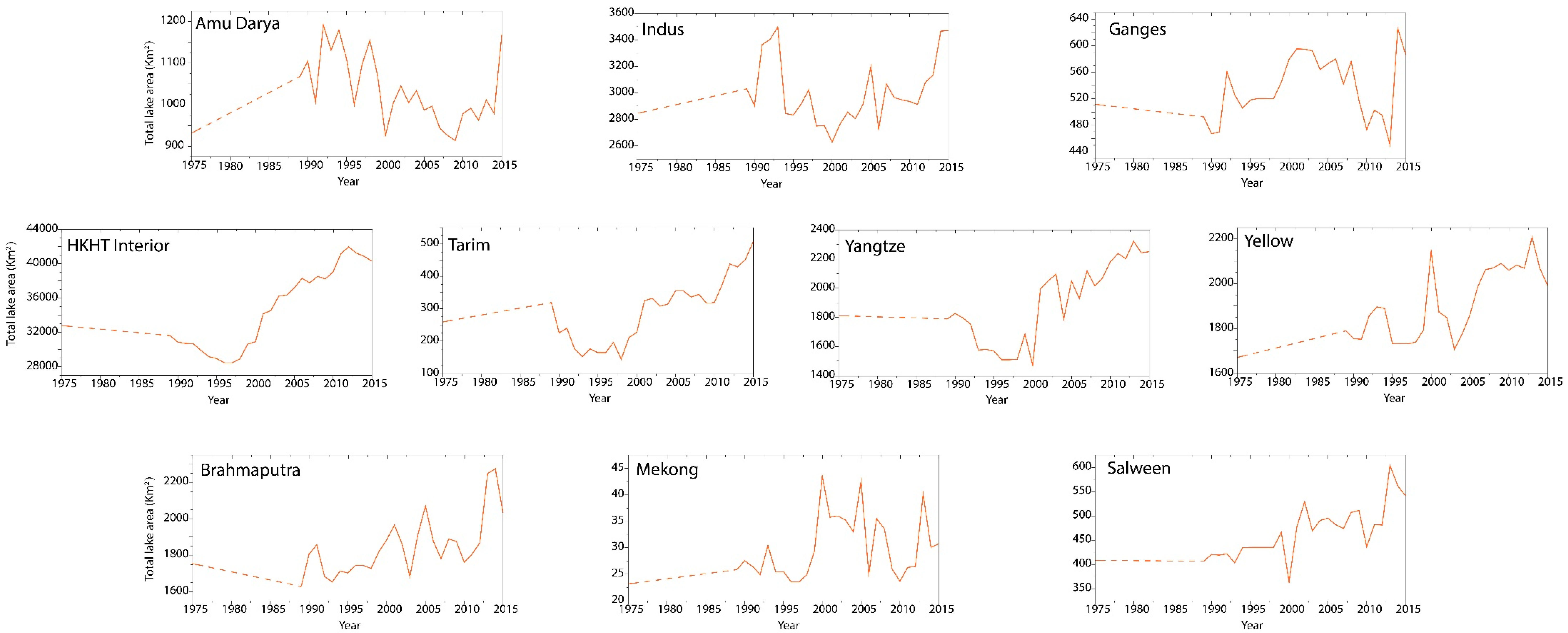
The results show that, during the first 20 years from the 1970s (~1975 to 1995), differences in lake changing patterns are apparent for different regions (Figure 4). The most intensive shrinkage was observed in northeastern HKHT (HKHT Interior, Tarim, and Yangtze) characterized by the greatest reduction in number of lakes (−56.3%, −34.0%, and −7.0%, respectively) and the lake surface area (−11.7%, −14.1%, and −13.3%, respectively). In contrast, extensive lake expansion was observed in the western and southwestern HKHT (Amu Darya, Ganges, Indus, and Brahmaputra) due to the proliferation of small lakes in high-altitude regions (154.9%, 267.3%, 162.2%, and 78.9%, respectively) (Figure 5). The total lake surface area started with a modest shrinking from of 43,006 (±668) km2 in the 1970s to 38,472 (±826) km2 in 1996, with a decrease of approximately 11.0%, followed by a rapid increase (~40.0%) from the lowest in 1996 to the highest point (53,702 ±707 km2) in 2013 (Figure 4). In the last three years, the total lake surface area decreased slightly from its peak in 2013, but still oscillated around 50,000 km2. The observed lake fluctuations are more drastic than previously reported [13,14,23], especially the observed decreasing trend in the 1990s. Despite the observed increasing trend in the upper Yellow basin in the first 20 years, if artificial lakes (such as Longyangxia Reservoir closed in 1992) built in this period are excluded, the lake area in the Yellow River basin was actually decreased by 192 km2 (~7.9%) in the same period.
The results indicated that the number of large lakes (surface area > 1 km2) in the HKHT regions decreased from 1196 in the 1970s to only 1009 in 1996, and then soared by 57.2%, peaking at 1586 in 2013. For instance, just in the HKHT Interior, Yangtze, Yellow, and Tarim basins, 202 (~22.0%) large lakes shrunk or disappeared in the first two decades. Despite the overall decreasing trend (490 large lakes shrunk by over 20%) in the four regions, 79 large lakes still experienced expansion. Among the 79 expanded lakes, 33 lakes are located in westerlies-affected regions, namely, Amu Darya, Indus, northern part of Ganges, and western part of Tarim. Another 46 lakes are in older glacial or permafrost landscapes (Figure 6). Smaller lakes (surface area < 1 km2) experienced a more significant fluctuation: 42.5% of small lakes were vanished in the aforementioned four regions, in contrast to the lakes in the Amu Darya, Indus, and Ganges basins where the number has almost doubled in the same period. In the next two decades, lake expansion is more pronounced—almost all basins experienced lake expansion—944 large lakes showed a significant increasing trend (>20% of increase in surface area) (Figure 7).
3.2. Possible Causes of Lake Fluctuation
The causes of lake fluctuation remain tangled due to elusive precipitation trends in the high-altitude regions [43,44]. The data indicates that temperature increases (0.1~0.6 per decade) in the HKHT regions are more pronounced compared to the lower elevation regions [1,45], thus leading to a rapid retreat of glaciers in recent decades [3,46]. Our results illustrated that the spatial and temporal characteristics of lake fluctuation and their responses to climate change and glacier retreat revealed three distinct patterns: (1) the impacts of the westerlies and glacier retreat in the Amu Darya, Indus, northern part of Ganges, and western part of Tarim, (2) the impacts of Indian summer monsoon (ISM) and glacier retreat in southern part of Ganges, Brahmaputra, Salween, and southern part of the HKHT Interior, and (3) the interplay of ISM and East Asian monsoon (EAM) in the Mekong, Yangtze, Yellow, and most part of the HKHT Interior (Figure 1 and Figure 4). Our results reflected previous reports about climatic controls on precipitation in the HKHT regions [47,48]. Despite the important role of glacial retreat in lake fluctuation, climate change (e.g., global warming or anomalous precipitation) was still the dominant force for lake fluctuations in the HKHT regions.
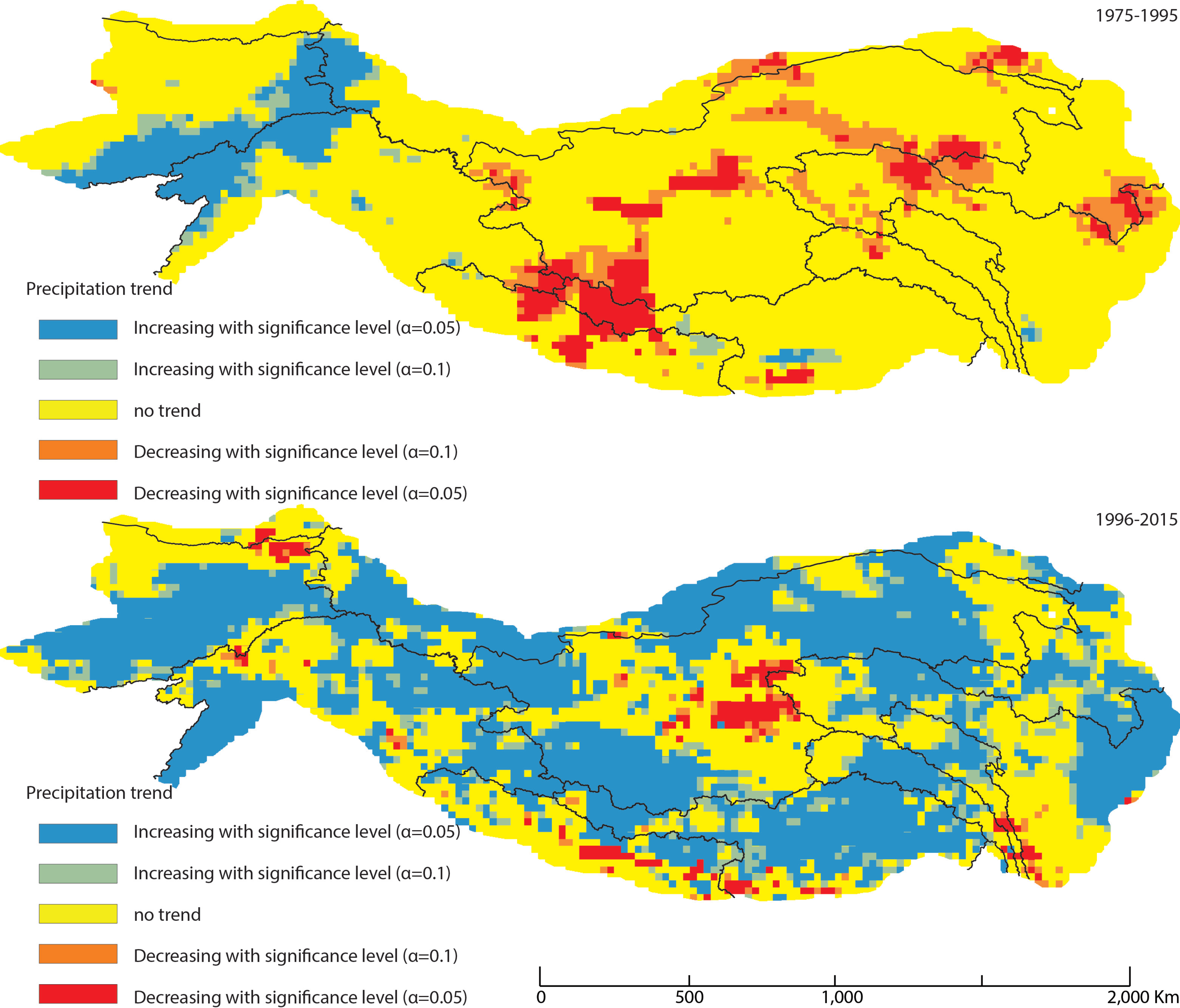
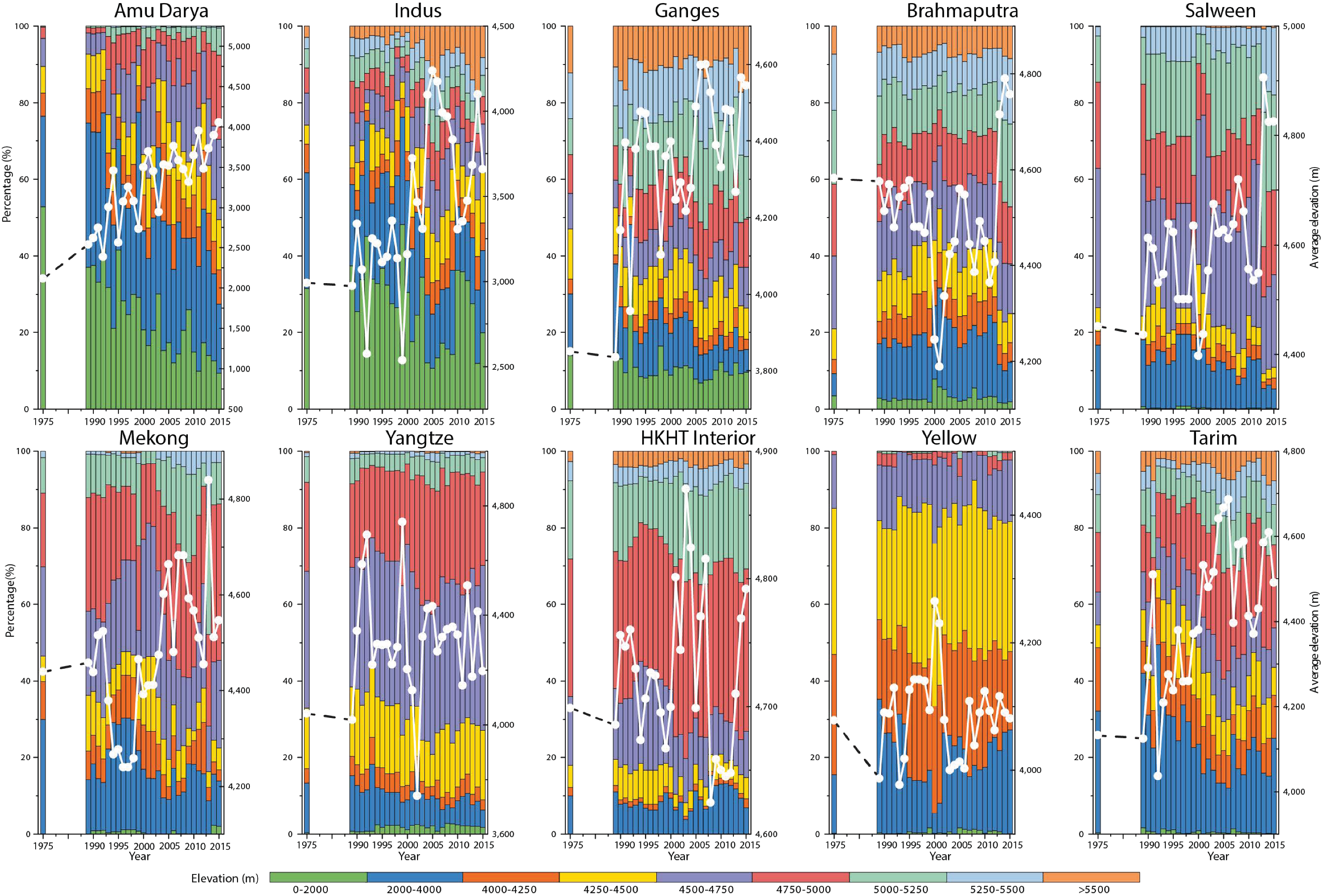
In the Amu Darya, Indus, northern part of Ganges, and western part of Tarim basins, which were affected by the westerlies and glacier retreat, increased precipitation in the 1990s (Figure 8) has caused expansions of lakes and glaciers in some areas [49]; however, after 2000 glacier retreat became more prominent, through the formation of numerous (glacial) lakes in high-altitude regions [21] resulting in the surge of average lake elevation (Figure 9). According to the lake fluctuation history for Amu Darya, Indus, Ganges, and Tarim in Figure 4, lake expansion in the westerlies affected basins is still significant in the second period (1992–2015), especially during the period after 2000. The Mann-Kendall (MK) Test (Figure 8) indicated that, in the first period (1975–1995), only the Amu Darya, Indus, northern part of Ganges, and western part of Tarim basins experienced an increasing trend in precipitation, followed by lake expansion correspondingly.
The fluctuation patterns in the region affected by ISM and glacier retreat genuinely indicated the interplay between climate change and glacier retreat, but the coupled effects were superimposed by short-term lake fluctuations before 2000 as the precipitation did not show any clear trend [50]. The surge in both number and average elevation of lakes, as opposed to the slight decreasing trend in precipitation after 2000 (Figure 9), indicated the impact of glacier retreat on lake creation.
In the region affected by the mixture of ISM and EAM, lake shrinking rate in the first period exhibited a gradient variation from north to south and from central west to east [51,52,53], but the lake expansion rate in the second period showed a reversed trend [14,23], which nearly aligned with the gradient change in spatial precipitation patterns. Regarding a relatively small number of glaciers in these areas (Table 2), inter-annual lake fluctuations are likely to directly relate to the annual precipitation variations, and hence are a better indicator of water balance change, especially in closed-basin lake systems. Decreased precipitation and resultant increased evaporation (especially in the HKHT Interior) were most likely the causes of lake shrinking in the early 1990s; while conversely, rapid lake expansion in the recent 20 years indicated increased precipitation and the climate change interplayed by the ISM and EAM [54].
3.3. Impact of Glacier Melt on Lake Fluctuations
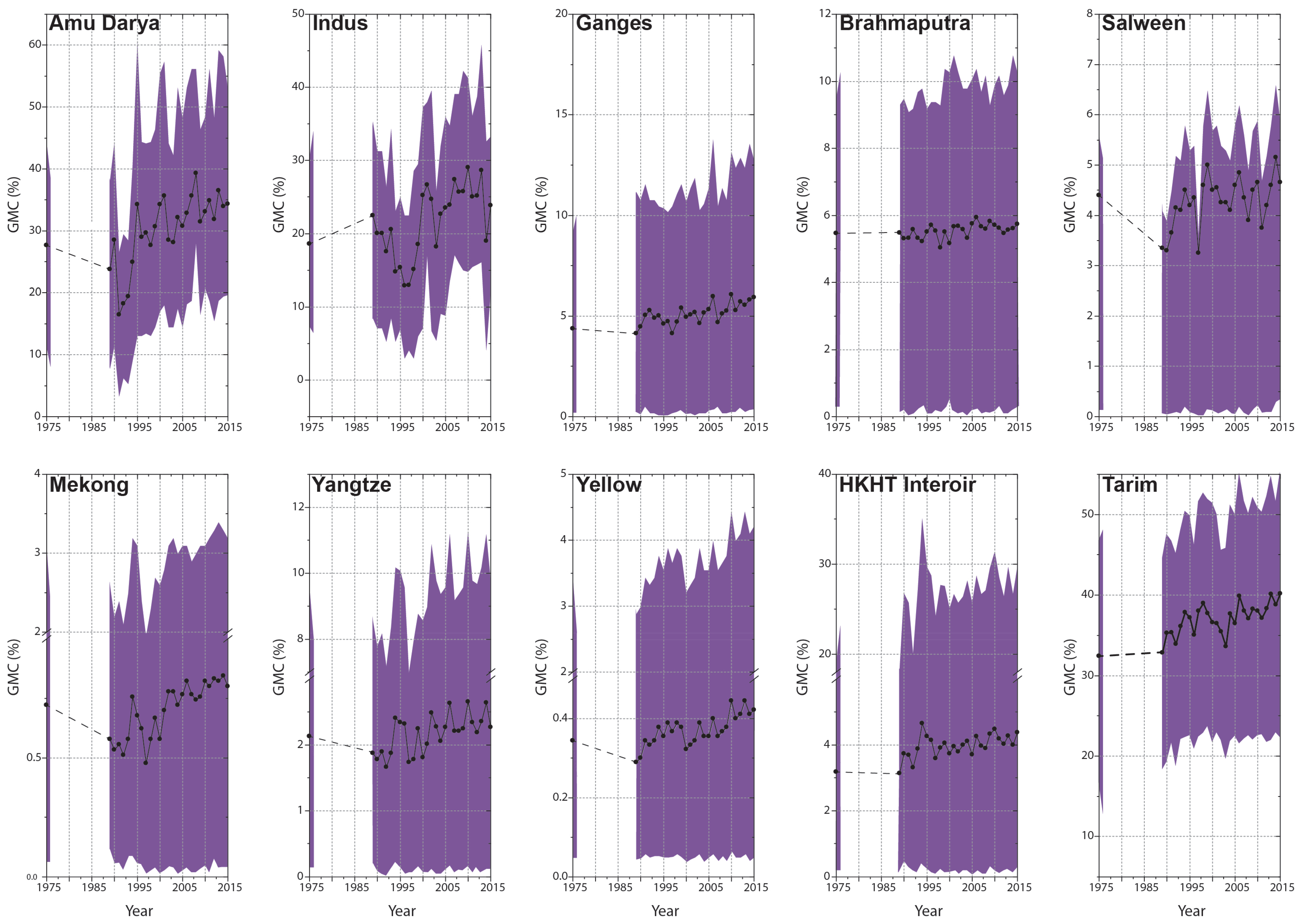
To discover the predominant driving forces to lake fluctuations, we selected 743 lake catchments (covering 65.6% of large lakes in the HKHT) to simulate glacier melt contribution (GMC) to water balance changes in each lake catchment during the period 1970s–2015. The annual GMC was determined by the averaged GMC values evaluated over the selected individual lake catchments within the river basin. The results, illustrated in Figure 10 and summarized by three periods in Table 1, indicate that the roles of precipitation and glaciers vary significantly over different basins and catchments. But the GMC to total lake annual flow has increased with varying degrees in almost all basins except the decrease during the period 1991–2000 in the westerlies-impacted Amu Darya and Indus basins.
In the arid Tarim basin, glacier runoff contribution to the flow makes 31.9~40.6%, the highest among the ten studied regions, indicating the key role of glacier melt in complementing deficient precipitation in the Tarim basin. In the Amu Darya and Indus basins, glacier runoff contributions to the annual lake flow make 16.5~39.3% and 12.8~29.0%, respectively, which are also of high importance to maintain water balance and to counteract high lake evaporation in summer. This is because in these basins, usually most of the precipitation occurs in winter and hence summer runoff mainly depends on glacier storage capacity [57]. Remarkably, although the absolute amount of temperature-driven glacier melt has continued to increase with slight fluctuations, the relative contribution is significantly disturbed by the precipitation fluctuations. For example, increased precipitation and relatively low temperature has weakened the contribution of glacier runoff in the Amu Darya basin in the 1990s [49].
The situation is converse in the HKHT Interior and the Yangtze basin, where precipitation-induced runoff is the predominant driving force, supplying 95.4~97.2% and 97.3~98.4% of lake water, respectively. The water short fall in the early 1990s and the significant water surplus after 2000 are mainly attributed to the precipitation fluctuations, which, in turn, influence the runoff into the lakes [35,58]. Indeed, only a small number of large lakes (e.g., Nam Co, Selin Co, and Zhari Nam Co) in the two basins are glacier-fed. Successive expansion of these lakes have been reported [15,22,59]. However, in the lake shrinking period 1990–1996, reduced precipitation (Figure 8) and resultant more cloud-free days have induced the highest GMC in 1994 in the HKHT Interior. Although EAM has been considerably intensified during the recent years and as a result, more precipitation could be transported to the plateau during the monsoon season in the past 20 years [60] (Figure 8). Raised temperature-induced glacier melt has grown even slightly faster. Despite the increasing trend of GMC after 1996, it still has not exceeded the peak of 1994. The combined effects favor coherently rapid lake expansion in both the HKHT Interior and the Yangtze basin.
In the Ganges basin, abundant annual precipitation (915~1360 mm yr−1 for the upstream area) is concentrated in summer, which predominantly determines the annual river flow [57]. This makes, in general, the contribution from the glacier melt relatively less significant (3.3–6.1%) to annual flow into lakes. However, glacier runoff can still be important for some lake catchments at high elevations (up to 14.2%). For example, in the Ganges basin, many lakes are located at high elevations and increased GMC indicated that the glacier melt affects hydrological cycles in lake catchments. The situation is similar in the Brahmaputra and Salween basins, the regions heavily influenced by summer monsoon. Glacier melt, which peaks in summer, is almost negligible in the high summer flow. In the Brahmaputra basin, for example, a relatively slow rise in air temperature (0.29ºC per decade) and small fluctuation in precipitation caused the contribution of glacier melt to lake run offs to be insignificant. Additionally, sublimation plays an important role in overall glacier ablation because of the low air humidity and prevalence of cloudless weather conditions [61], which consequently reduce the meltwater discharge from glaciers to lakes.
Our study also demonstrated dramatic anthropogenic impacts on lake fluctuations in the Yellow River basin that have been rarely reported in previous studies. The damming of the Gyaring and Ngorning lakes at 4300 m above sea level and the construction of the Longyangxia reservoir at 2700 m and 11 other large artificial lakes in the upstream reaches have notably disturbed natural lake evolution in recent decades. In contrast to a sharp increase in artificial lakes, rapidly shrinking natural lakes will undoubtedly degrade and interrupt local lake wetland ecosystems and water security issues.
4. Discussion
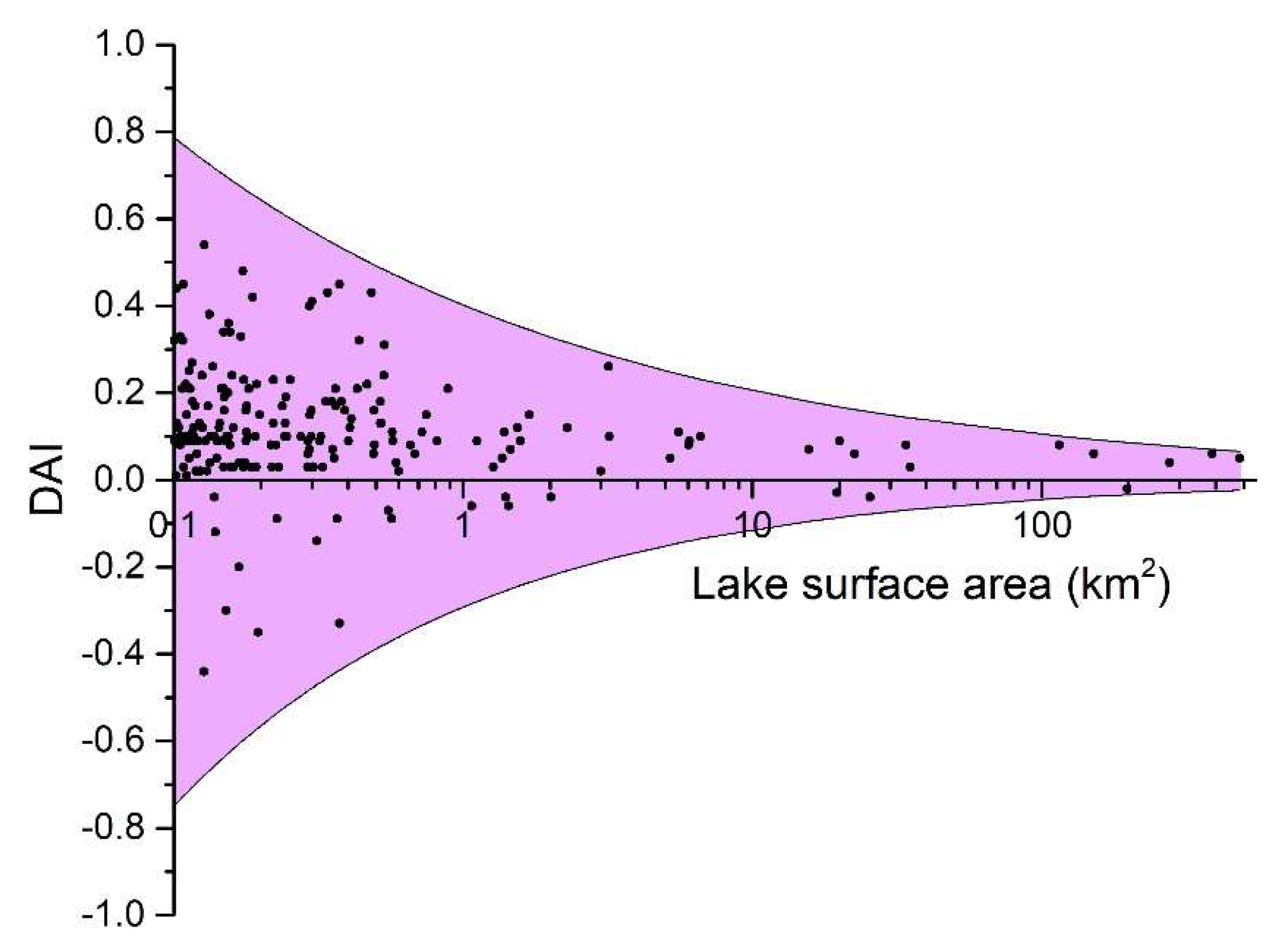
The accuracy of lake delineation was primarily influenced by image quality such as resolution, cloud cover, and shadows. For example, mixed pixels made some small lakes difficult to be extracted. Although the SRTM DEM data was used to identify and remove shadows, the effects could not be completely removed. The results indicated that most of DAI values vary between −0.3 and 0.3 (Figure 11) indicating that the two datasets match well. With the increase of the surface area, the absolute values of DAI become close to zero, indicating that the larger lakes are more accurately delineated. The results also showed that more DAI values for small water bodies were greater than zero, indicating that small water bodies delineated in high-resolution images were slightly larger than their corresponding area derived from Landsat images. This is not surprising, because in Landsat images only the lakes with inlets larger than 30 m (60 m for MSS imagery) could be identified. Although the accuracy for small lakes (<1 km2) is relatively low, lakes with area greater than 1 km2 contribute 93±2.8% to the total surface area. Therefore, the relatively low accuracy for small water bodies has minimal impact on area-based analysis.
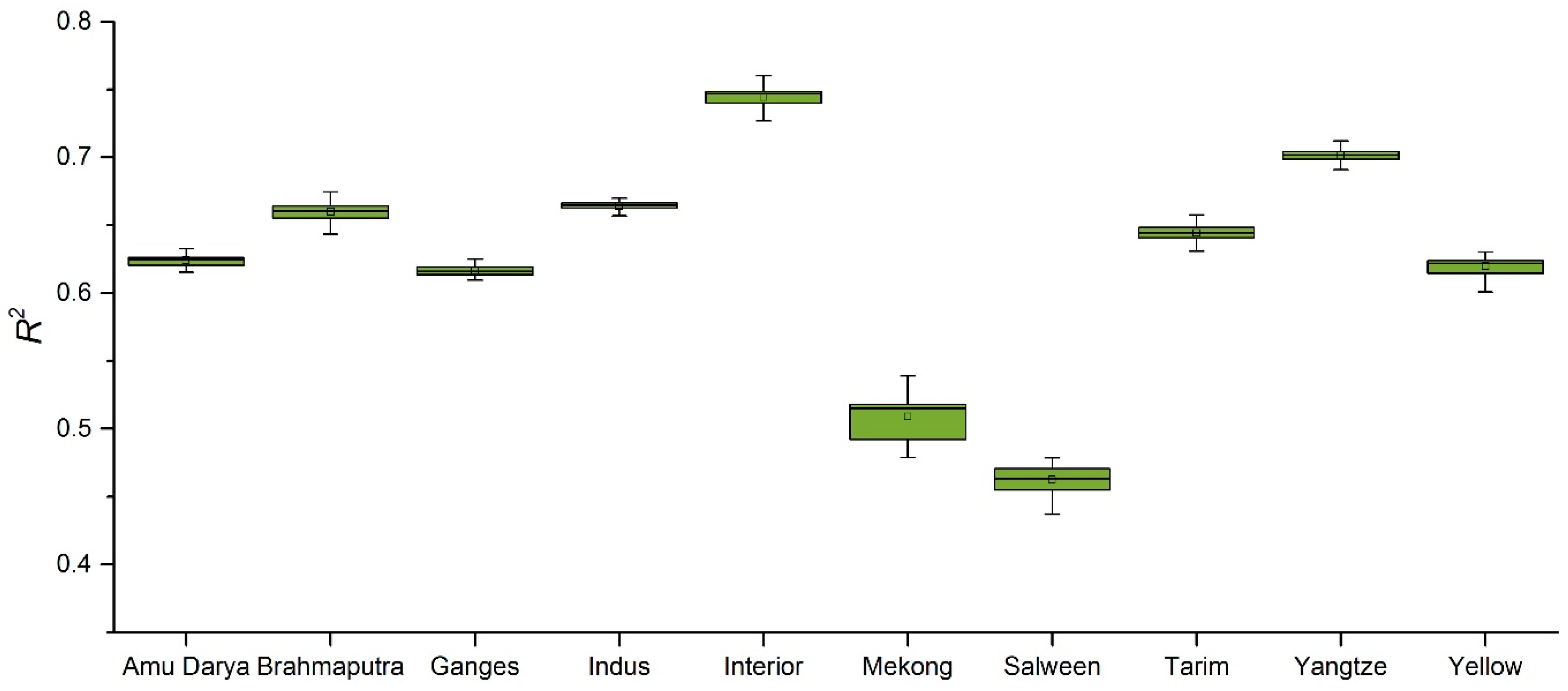
We used RMR runoff models (see the methodology section) for cross validation of regression models. The adjusted values for the ten regressions to estimate the annual runoff based on climatic and physical characteristics vary from 0.74 for the HKHT Interior basin to 0.46 for the Salween River, with an average of 0.63 (Figure 12 and Table 3). The R2 values for the Salween and Mekong basins are relatively low because of too small sample size (n = 24 and 10, respectively). The uncertainty in the RMR runoff models is primarily related to the reliability of the simulated physical and climatic characteristics of catchments. For example, the climatic characteristics determine the overall uncertainty of glacier runoff estimation. However, compared to other populated regions, currently available meteorological records for high mountains in remote areas are sparse and do not well capture the rapidly changing alpine climate [62,63]. Accuracy of some of the meteorological forcing datasets used in this study (i.e., APHRODITE, TRMM, and GLDAS) also may not be sufficient, particularly for precipitation. Although they reflect orographic and rain shadow effects, they are not ideal for reproducing the effects of wind and snow avalanches, which might play an essential role in the alpine settings as a surrogate of snow relocation [64]. Relying on the rugged alpine topography, any concave shape in the mountains becomes an efficient trap for preferential snow accumulation, in many areas sustaining a glacier. As a result, glacier runoff in some lake catchments may be much higher than other glaciated areas. These exceptional snow relocation and resulting glacier mass changes remain a challenge to be handled by process-based models. For some small- and medium-sized lake catchments, these effects might become even more significant. However, these exceptions are reflected in the lake fluctuations, thus we used RMR analyses to estimate glacier runoff.
In Table 3, it can be seen that the key factors affecting runoff are catchment area (CA) and rainfall (P); these two factors show a good positive correlation with runoff. Both of the two factors are involved in the ten regression models. There are also several factors that are negatively correlated with runoff, such as temperature (T and Tmax) and evaporation (ET). Since the environment in alpine regions is extremely sensitive to climate change, an increase in temperature means an enhance in evaporation, which in turn leads to a drop-in runoff. At the same time, from these ten models, we can also see the different configuration in regression models due to the variations in rainfall pattern. For example, in the Amu Darya basin, affected by the westerlies, rainfall mainly occurred in winter, but ET is the highest in summer. The regression model for the Amu Darya basin is a good representative of the interplay between temperature and rainfall on runoff generation.
According to the meteorological data, spatial variability of precipitation in the upper reaches of the large rivers is in the range of 300–3000 mm in the Ganges and Brahmaputra basins, 250–2500 mm in the Amu Darya and Indus basins, as well as 50–1000 mm in the HKHT Interior. The condition is similar for air temperature. Since the variability of precipitation over short distances is very high, a reliable assessment of the amount of precipitation received by a small- to medium-sized lake catchments is challenging. For that we used lapse rate approaches to calibrate the datasets, however, the highly variable precipitation and temperature over space were still the major limitation in inaccurately predicting the temperature and precipitation from ground observations.
In addition, the GMC for each river basin was an averaged value over the selected lake catchments. However, due to the extremely uneven lake distribution in the HKHT regions, small sample size of lakes in the Mekong, and Salween could have introduced some uncertainties in the assessment of GMC impacts on lake fluctuations. Additionally, using climatological data from different sources and the uncertainty in delineating the lake surface area from satellite images could also have influenced the assessment. Figure 12 shows that, even within the same river basin, the GMC values vary greatly depending on the glaciered area in the lake catchments. Therefore, we assessed an overall trend for each of the whole river basins in the HKHT regions, rather than the individual lake catchments.
Compared with previous studies, this study illustrates some new discoveries. First, many studies, including Mao, Wang [20], Zhang, Yao [23], and this study, reported lake shrinkage from the 1970s to 1990s, followed by a period of lake expansion after 1990s, but the first two studies [20,23] did not provide the exact time when the lakes in the HKHT regions changed from shrinkage to expansion; while this study concluded that the transformation from shrinkage to expansion happened during 1995 to 1996. The number of large lakes (> 1km2) bottomed at 1009 in 1996, instead of 1109 in 1990 by Mao, Wang [20] or 1070 in 1990 by Zhang, Yao [23]. It should be noted that the studies by Mao, Wang [20] and Zhang, Yao [23] investigated only the HKHT region within China, excluding the HKHT regions within Afghanistan, Pakistan, Nepal, India, and other countries. If such regions are included, the difference will be more significant. Second, the previous studies [13,20,23] only reported steady lake expansion after the 1990s, but they failed to identify the peak of lake expansion in 2013 and the slight drop from 2013 to 2014. Third, previous studies [13,14,15,17,18,19,20] have discussed the driving forces for lake fluctuations, such as climatic factors, glacier retreat, permafrost degradation, but only a few quantitative assessments were conducted regarding these factors. The direct effects on lake fluctuations still remain largely unknown. The study assessed the role of glacier retreat on lake fluctuations and quantified the glacier melt contribution to lake water balance changes in different regions and reported the large variation in glacier melt contribution across the HKHT regions.
In addition, it should be noted that, some other factors (e.g., permafrost degradation) should not be ignored in some areas. For example, hundreds of thermokarst lakes are spread in the HKHT Interior region and the headwater region of the Yangtze. Based on the spatial distribution of permafrost and temperature changes, permafrost degradation was most pronounced between the Himalayas and Tanggula Mountains [20]. Although few studies have been conducted to investigate the relationships between climatic variables, permafrost cover, and water balance of high-elevation inland lakes, due to the lack of glaciological, geocryological, and hydrological information [65], the impact of permafrost degradation on lake fluctuations should be highly emphasized in future studies.
5. Conclusions
Overall, our findings show that climate change and resultant glacier retreat has led to dramatic changes in number of lakes, lake surface area, and their vertical distribution in the HKHT regions, although the patterns of these changes are distinct from region to region. The results indicate that glacier melt plays a critical role in the hydrological cycle by maintaining lake water balance in the Amu Darya, Indus, and Tarim basins, but that was a negligible component in the lake water balances in the HKHT Interior, Yangtze, and Yellow river basins. Our observations corroborate the previous findings [54] that the most extreme glacial shrinkage occurred in the Himalayas with reduction in both the glacier length and area, and for that the meltwater is important in sustaining water availability in the Amu Darya, Indus, and Tarim basins [6,9,66]. Previous studies [6,51,60,61] have reported the rising river flows due to glacier retreat in the HKHT regions. However, our results showed that the river flows and GMC fluctuations have no consistent trends but rather they are mainly controlled by the changing climate, especially the precipitation (despite the significant differences in precipitation patterns over basins and catchments) [44]. In the rainfall-runoff-dominated HKHT Interior and Yellow River basin, the insufficient precipitation has derived two contradictory trends: Increased GMC but decreased flows and shrinking lakes in the same period. These inconsistent trends could make water availability in these regions highly vulnerable especially over the long term, implying the necessity of further research on this topic. As GMC consistently increased in the Tarim, Ganges, and Brahmaputra basins, it is essential to tackle extreme events and their inter-annual effects on downstream water availability. Changes in the frequency of extreme events may increase the risk of natural flooding in the middle and lower reaches of the Ganges and Brahmaputra rivers, while inter-annual shifts in downstream water availability may consequently affect the regional food security in the arid Tarim basin where flow peaks and growing seasons are not coinciding. The findings in this study may thus present both immediate and long-term policy implications for dealing with water-related hazards, controlling glacial lake outburst floods, securing water availability, protecting lake wetlands, and assessing regional climate change and resultant glacier retreat in the HKHT regions.
Author Contributions
Conceptualization and Methodology, X.Y., X.L., P.T., Data analysis, X.Y., Writing-Original Draft Preparation, X.Y., Writing & Editing, X.L. E.P. and P.T.
Acknowledgments
The authors would like to acknowledge the financial support from the National Natural Science Foundation of China (grant Nos. 41871017 and 91547110), and the research support from the Guangzhou University (grant No. 69-18ZX1000201). E.P. would like to acknowledge the Earth Observatory of Singapore.
Conflicts of Interest
The authors declare no conflict of interest.
References
- Solomon, S.; Qin, D.; Manning, M.; Chen, Z.; Marquis, M.; Averyt, K.; Tignor, M.; Miller, H. IPCC, Climate Change 2007: The Physical Science Basis; Cambridge University Press: Cambridge, UK, 2007. [Google Scholar]
- Barnett, T.P.; Adam, J.C.; Lettenmaier, D.P. Potential impacts of a warming climate on water availability in snow-dominated regions. Nature 2005, 438, 303–309. [Google Scholar] [CrossRef] [PubMed]
- Bolch, T.; Kulkarni, A.; Kaab, A.; Huggel, C.; Paul, F.; Cogley, J.G.; Frey, H.; Kargel, J.S.; Fujita, K.; Scheel, M.; et al. The State and Fate of Himalayan Glaciers. Science 2012, 336, 310–314. [Google Scholar] [CrossRef] [PubMed] [Green Version]
- Shi, Y.F.; Shen, Y.P.; Kang, E.; Li, D.L.; Ding, Y.J.; Zhang, G.W.; Hu, R.J. Recent and future climate change in northwest china. Climat. Chang. E 2007, 80, 379–393. [Google Scholar] [CrossRef]
- Ji, J.F.; Shen, J.; Balsam, W.; Chen, J.; Liu, L.W.; Liu, X.Q. Asian monsoon oscillations in the northeastern Qinghai-Tibet Plateau since the late glacial as interpreted from visible reflectance of Qinghai Lake sediments. Earth. Planet. Sc. Lett 2005, 233, 61–70. [Google Scholar] [CrossRef]
- Immerzeel, W.W.; Van Beek, L.P.; Bierkens, M.F. Climate change will affect the Asian water towers. Science 2010, 328, 1382–1385. [Google Scholar] [CrossRef] [PubMed]
- Kohler, T.; Pratt, J.; Debarbieux, B.; Balsiger, J.; Rudaz, G.; Maselli, D. Sustainable Mountain Development, Green Economy and Institutions. From Rio 1992 to Rio 2012 and Beyond; International Centre for Integrated Mountain Development (ICIMOD): Kathmandu, Nepal, 2012. [Google Scholar]
- Beniston, M. Climatic change in mountain regions: A review of possible impacts. In Climate Variability and Change in High Elevation Regions: Past, Present & Future; Henry, F.D., Martin, G., Lisa, J.G., Eds.; Springer: Berlin, Germany, 2003; pp. 5–31. [Google Scholar]
- Yao, T.; Wang, Y.; Liu, S.; Pu, J.; Shen, Y.; Lu, A. Recent glacial retreat in High Asia in China and its impact on water resource in Northwest China. Sci. China Seri. D: Earth Sci. 2004, 47, 1065–1075. [Google Scholar] [CrossRef]
- IPCC. Summary for Policymakers. In Climate Change 2007: The Physical Science Basis; Solomon, S., Qin, D., Manning, M., Chen, Z., Marquis, M., Averyt, K., Tignor, M., Miller, H., Eds.; Cambridge University Press: Cambridge, UK, 2007; pp. 1–18. [Google Scholar]
- Richardson, S.D.; Reynolds, J.M. An overview of glacial hazards in the Himalayas. Quatern. Int. 2000, 65, 31–47. [Google Scholar] [CrossRef]
- Xu, J.; Grumbine, R.E.; Shrestha, A.; Eriksson, M.; Yang, X.; Wang, Y.; Wilkes, A. The melting Himalayas: Cascading effects of climate change on water, biodiversity, and livelihoods. Conserv. Biol. 2009, 23, 520–530. [Google Scholar] [CrossRef]
- Song, C.Q.; Huang, B.; Ke, L.H. Modeling and analysis of lake water storage changes on the Tibetan Plateau using multi-mission satellite data. Remote Sens. Environ. 2013, 135, 25–35. [Google Scholar] [CrossRef]
- Lei, Y.B.; Yang, K.; Wang, B.; Sheng, Y.W.; Bird, B.W.; Zhang, G.Q.; Tian, L.D. Response of inland lake dynamics over the Tibetan Plateau to climate change. Climat. Change. 2014, 125, 281–290. [Google Scholar] [CrossRef]
- Zhou, J.; Wang, L.; Zhang, Y.; Guo, Y.; Li, X.; Liu, W. Exploring the water storage changes in the largest lake (Selin Co) over the Tibetan Plateau during 2003–2012 from a basin-wide hydrological modeling. Water Resour. Res. 2015, WR015846. [Google Scholar] [CrossRef]
- Yasuda, T.; Furuya, M. Short-term glacier velocity changes at West Kunlun Shan, Northwest Tibet, detected by Synthetic Aperture Radar data. Remote Sens. Environ. 2013, 128, 87–106. [Google Scholar] [CrossRef] [Green Version]
- Gardelle, J.; Arnaud, Y.; Berthier, E. Contrasted evolution of glacial lakes along the Hindu Kush Himalaya mountain range between 1990 and 2009. Global Planet. Change 2011, 75, 47–55. [Google Scholar] [CrossRef] [Green Version]
- Khadka, N.; Zhang, G.; Thakuri, S. Glacial Lakes in the Nepal Himalaya: Inventory and Decadal Dynamics (1977–2017). Remote Sens. 2018, 10, 1913. [Google Scholar] [CrossRef]
- Kulkarni, A.V.; Rathore, B.; Singh, S.; Bahuguna, I. Understanding changes in the Himalayan cryosphere using remote sensing techniques. Int. J. Remote. Sens. 2011, 32, 601–615. [Google Scholar] [CrossRef]
- Mao, D.; Wang, Z.; Yang, H.; Li, H.; Thompson, J.; Li, L.; Song, K.; Chen, B.; Gao, H.; Wu, J. Impacts of climate change on Tibetan lakes: Patterns and processes. Remote Sens. 2018, 10, 358. [Google Scholar] [CrossRef]
- Mergili, M.; Müller, J.P.; Schneider, J.F. Spatio-temporal development of high-mountain lakes in the headwaters of the Amu Darya River (Central Asia). Global Planet. Change 2013, 107, 13–24. [Google Scholar] [CrossRef]
- Yang, X.K.; Lu, X.X. Drastic change in China’s lakes and reservoirs over the past decades. Sci. Rep. 2014, 4, 6041. [Google Scholar] [CrossRef] [PubMed]
- Zhang, G.Q.; Yao, T.D.; Xie, H.J.; Zhang, K.X.; Zhu, F.J. Lakes’ state and abundance across the Tibetan Plateau. Chinese. Sci. Bull. 2014, 59, 3010–3021. [Google Scholar] [CrossRef]
- NASA. Landsat 7 Science Data Users Handbook. 2011. Available online: https://landsat.gsfc.nasa.gov/wp-content/uploads/2016/08/Landsat7_Handbook.pdf (accessed on 7 May 2019).
- MWR. Standard of the People’s Republic of China: Code for China Lake Name; China Water Power Press: Beijing, China, 1998. [Google Scholar]
- Wang, S.; Dou, H. Chinese Lake Catalogue; Science Press: Beijing, China, 1998; p. 580. [Google Scholar]
- Yatagai, A.; Kamiguchi, K.; Arakawa, O.; Hamada, A.; Yasutomi, N.; Kitoh, A. APHRODITE: Constructing a long-term daily gridded precipitation dataset for Asia based on a dense network of rain gauges. B. Am. Meteorol. Soc. 2012, 93, 1401–1415. [Google Scholar] [CrossRef]
- Woodcock, C.E.; Allen, R.; Anderson, M.; Belward, A.; Bindschadler, R.; Cohen, W.; et al. Free access to Landsat imagery. Science 2008, 320, 1011. [Google Scholar] [CrossRef]
- GLIMS, NSIDC. GLIMS Glacier Database, Version 1. Available online: https://nsidc.org/data/NSIDC-0272 (accessed on 7 May 2019).
- Farr, T.G.; Rosen, P.A.; Caro, E.; Crippen, R.; Duren, R.; Hensley, S.; Kobrick, M.; Paller, M.; Rodriguez, E.; Roth, L. The shuttle radar topography mission. Rev. Geophys. 2007, 45, RG2004. [Google Scholar] [CrossRef]
- Minder, J.R.; Mote, P.W.; Lundquist, J.D. Surface temperature lapse rates over complex terrain: Lessons from the Cascade Mountains. J. Geophys. Res.: Atmos. 2010, 115, D14122. [Google Scholar] [CrossRef]
- Pal, M.; Mather, P. Support vector machines for classification in remote sensing. Int. J. Remote. Sens. 2005, 26, 1007–1011. [Google Scholar] [CrossRef]
- Mountrakis, G.; Im, J.; Ogole, C. Support vector machines in remote sensing: A review. Isprs, J. Photogramm. 2011, 66, 247–259. [Google Scholar] [CrossRef]
- Bishop, C.M. Pattern Recognition and Machine Learning; Springer: Berlin, Germany; 2006. [Google Scholar]
- Yang, X.K.; Lu, X.X. Delineation of lakes and reservoirs in large river basins: An example of the Yangtze River Basin, China. Geomorphology 2013, 190, 92–102. [Google Scholar] [CrossRef]
- Scaramuzza, P.; Micijevic, E.; Chander, G. SLC Gap-Filled Products Phase One Methodology; Geological Survey: Bassett, VA, USA, 2004.
- Lehner, B.; Liermann, C.R.; Revenga, C.; Voeroesmarty, C.; Fekete, B.; Crouzcet, P.; Doell, P.; Endejan, M.; Frenken, K.; Magome, J.; et al. High-resolution mapping of the world’s reservoirs and dams for sustainable river-flow management. Front. Ecology Environ. 2011, 9, 494–502. [Google Scholar] [CrossRef]
- Penman, H.L. Natural evaporation from open water, bare soil and grass. Math. Phys. Eng. Sci. 1948, 193, 120–146. [Google Scholar]
- Blöschl, G. Runoff Prediction in Ungauged Basins: Synthesis across Processes, Places and Scales; Cambridge University Press: Cambridge, UK, 2013; p. 490. [Google Scholar]
- Driver, N.E.; Troutman, B.M. Regression models for estimating urban storm-runoff quality and quantity in the United States. J. Hydrol. 1989, 109, 221–236. [Google Scholar] [CrossRef]
- Vogel, R.M.; Wilson, I.; Daly, C. Regional regression models of annual streamflow for the United States. J. Irrigation Drain. Eng. 1999, 125, 148–157. [Google Scholar] [CrossRef]
- Hernandez, M.; Miller, S.N.; Goodrich, D.C.; Goff, B.F.; Kepner, W.G.; Edmonds, C.M.; Jones, K.B. Modeling Runoff Response to Land Cover and Rainfall Spatial Variability in Semi-Arid Watersheds; Springer: Berlin, Germany, 2000; pp. 285–298. [Google Scholar]
- Palazzi, E.; Hardenberg, J.; Provenzale, A. Precipitation in the Hindu-Kush Karakoram Himalaya: Observations and future scenarios. J. Geophys. Res. Atmos. 2013, 118, 85–100. [Google Scholar] [CrossRef] [Green Version]
- Li, M.; Wu, J.; Song, C.; He, Y.; Niu, B.; Fu, G.; et al. Temporal Variability of Precipitation and Biomass of Alpine Grasslands on the Northern Tibetan Plateau. Remote Sens. 2019, 11, 360. [Google Scholar] [CrossRef]
- Singh, S.P.; Bassignana-Khadka, I.; Karky, B.S.; Sharma, E. Climate Change in the Hindu Kush-Himalayas: The State of Current Knowledge; International Centre for Integrated Mountain Development (ICIMOD): Kathmandu, Nepal, 2011; p. 102. [Google Scholar]
- Laghari, J.R. Climate change: Melting glaciers bring energy uncertainty. Nature 2013, 503, 464. [Google Scholar] [CrossRef]
- Yao, T.; Masson-Delmotte, V.; Gao, J.; Yu, W.; Yang, X.; Risi, C.; Sturm, C.; Werner, M.; Zhao, H.; He, Y. A review of climatic controls on δ18O in precipitation over the Tibetan Plateau: Observations and simulations. Rev. Geophys. 2013, 51, 525–548. [Google Scholar] [CrossRef] [Green Version]
- Benn, D.; Owen, L. The role of the Indian summer monsoon and the mid-latitude westerlies in Himalayan glaciation: Review and speculative discussion. J. Geol. Soc. London. 1998, 155, 353–363. [Google Scholar] [CrossRef]
- Hewitt, K. The Karakoram anomaly? Glacier expansion and the ’elevation effect,’ Karakoram Himalaya. Mount. Res. Develop. 2005, 25, 332–340. [Google Scholar] [CrossRef]
- Immerzeel, W. Historical trends and future predictions of climate variability in the Brahmaputra basin. Int. J. Climatol. 2008, 28, 243. [Google Scholar] [CrossRef]
- Lutz, A.; Immerzeel, W.; Shrestha, A.; Bierkens, M. Consistent increase in High Asia’s runoff due to increasing glacier melt and precipitation. Nature Climate Change 2014, 4, 587–592. [Google Scholar] [CrossRef]
- Anders, A.M.; Roe, G.H.; Hallet, B.; Montgomery, D.R.; Finnegan, N.J.; Putkonen, J. Spatial patterns of precipitation and topography in the Himalaya. Geolog. Soc. Am. Special Papers 2006, 398, 39–53. [Google Scholar]
- Hudson, A.M.; Quade, J. Long-term east-west asymmetry in monsoon rainfall on the Tibetan Plateau. Geology 2013, 41, 351–354. [Google Scholar] [CrossRef]
- Yao, T.D.; Thompson, L.; Yang, W.; Yu, W.S.; Gao, Y.; Guo, X.J.; Yang, X.X.; Duan, K.Q.; Zhao, H.B.; Xu, B.Q.; et al. Different glacier status with atmospheric circulations in Tibetan Plateau and surroundings. Nature Climate Change 2012, 2, 663–667. [Google Scholar] [CrossRef]
- Watersheds of the World. Available online: https://www.wri.org/publication/watersheds-world (accessed on 7 May 2019).
- Xu, J.; Arun, S.; Rameshananda, V.; Mats, E.; Kenneth, H. The Melting Himalayas; International Center for Integrated Mountain Development (ICIMOD): Kathmandu, Nepal, 2007. [Google Scholar]
- Kaser, G.; Grosshauser, M.; Marzeion, B. Contribution potential of glaciers to water availability in different climate regimes. Proc. Natl. Acad. Sci. USA 2010, 107, 20223–20227. [Google Scholar] [CrossRef]
- Yang, K.; Wu, H.; Qin, J.; Lin, C.G.; Tang, W.J.; Chen, Y.Y. Recent climate changes over the Tibetan Plateau and their impacts on energy and water cycle: A review. Global Planet. Change 2014, 112, 79–91. [Google Scholar] [CrossRef]
- Wu, Y.H.; Zhu, L.P. The response of lake-glacier variations to climate change in Nam Co Catchment, central Tibetan Plateau, during 1970-2000. J. Geograph. Sci. 2008, 18, 177–189. [Google Scholar] [CrossRef]
- Wang, B.; Liu, J.; Kim, H.J.; Webster, P.J.; Yim, S.Y.; Xiang, B.Q. Northern Hemisphere summer monsoon intensified by mega-El Nino/southern oscillation and Atlantic multidecadal oscillation. Proc. Natl. Acad. Sci. USA 2013, 110, 5347–5352. [Google Scholar] [CrossRef]
- Savoskul, O.S.; Smakhtin, V. Glacier Systems and Seasonal Snow Cover in Six Major Asian River Basins: Hydrological Role Under Changing Climate; International Water Management Institude (IWMI): Colombo, Sri Lanka, 2013; p. 45. [Google Scholar]
- Archer, D. Contrasting hydrological regimes in the upper Indus Basin. J. Hydrol. 2003, 274, 198–210. [Google Scholar] [CrossRef]
- Fowler, H.; Archer, D. Conflicting signals of climatic change in the Upper Indus Basin. J. Climate 2006, 19, 4276–4293. [Google Scholar] [CrossRef]
- Young, G.; Hewitt, K. Hydrology research in the upper Indus basin, Karakoram Himalaya, Pakistan. Hydrol. Mount. Areas. IAHS Publ. 1990, 190, 139–152. [Google Scholar]
- Liu, J.; Kang, S.; Gong, T.; Lu, A. Growth of a high-elevation large inland lake, associated with climate change and permafrost degradation in Tibet. Hydrol. Earth Sys. Sci. 2010, 14, 481–489. [Google Scholar] [CrossRef] [Green Version]
- Jacob, T.; Wahr, J.; Pfeffer, W.T.; Swenson, S. Recent contributions of glaciers and ice caps to sea level rise. Nature 2012, 482, 514–518. [Google Scholar] [CrossRef]
Figure 1.
Geographical settings of the Amu Darya, Tarim, Indus, Ganges, Brahmaputra, Salween, Mekong, Yangtze, Yellow rivers, and Hindu Kush-Himalaya-Tibetan (HKHT) Interior (also known as Tibetan Plateau Interior). The blue, orange, and black arrows depict that climate change in the HKHT regions was revealed by three distinct patterns: (1) Amu Darya, Indus, northern part of Ganges, and western part of Tarim associated with the impact of the westerlies, (2) Brahmaputra, Salween, and southern part of Ganges controlled by the Indian summer monsoon (ISM), and (3) Mekong, Yangtze, Yellow, and most part of the HKHT Interior resulted from the mix of ISM and Eastern Asian monsoon (EAM).

Figure 2.
Stacked bar graph of the number of Landsat images used for each year by image data sources.
Figure 2.
Stacked bar graph of the number of Landsat images used for each year by image data sources.

Figure 3.
A representative example of lake gap-fill results, using Landsat ETM+ bands 3, 2, 1.

Figure 4.
Lake fluctuation history over the period 1975–2015 showing an annual lake fluctuation observed from remote sensing for the corresponding large river basins. No satellite imagery is available for the period 1976–1988 and this gap is represented by dash line.
Figure 4.
Lake fluctuation history over the period 1975–2015 showing an annual lake fluctuation observed from remote sensing for the corresponding large river basins. No satellite imagery is available for the period 1976–1988 and this gap is represented by dash line.

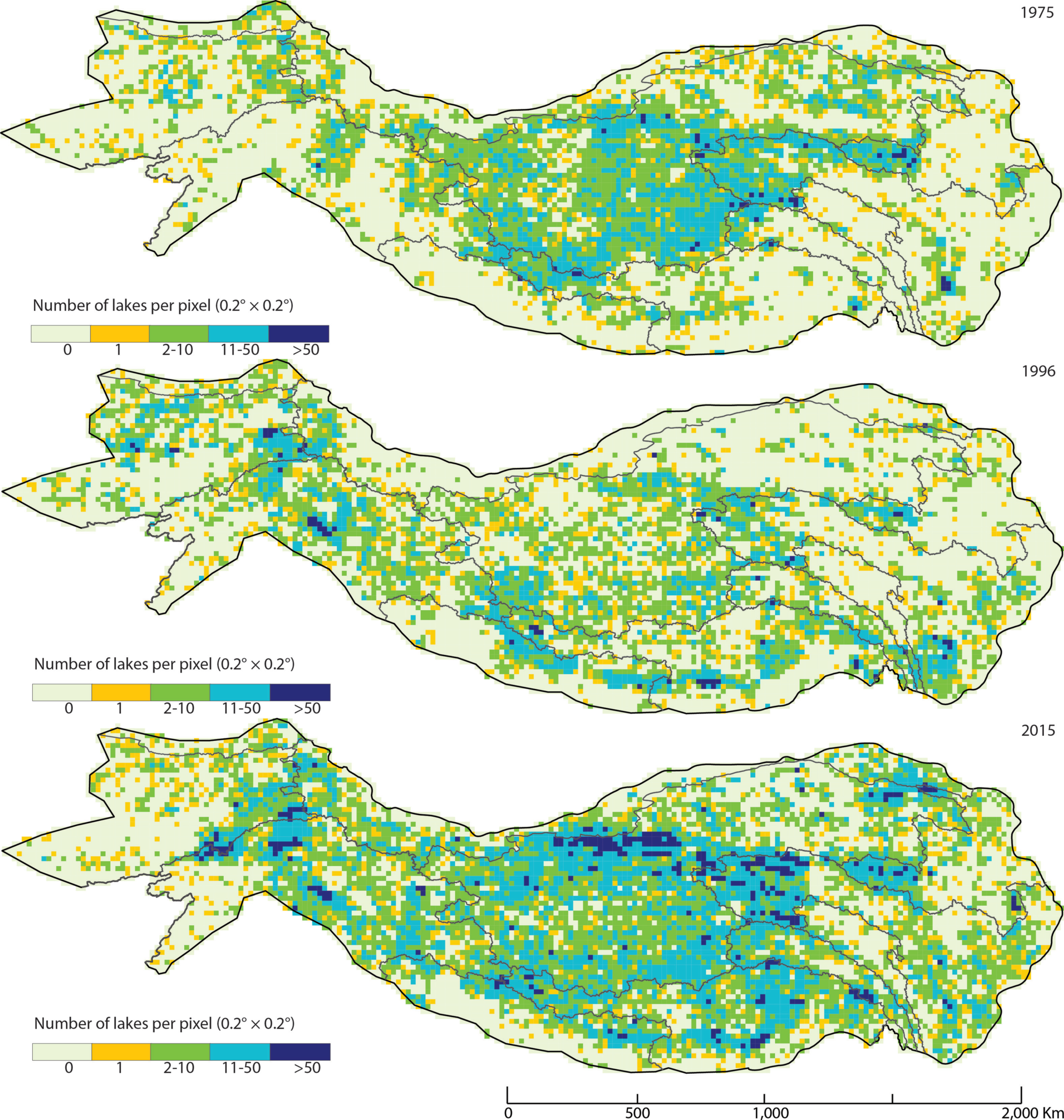
Figure 5.
Lake density variation across the HKHT regions for the three important milestone years 1975 (initial status with 44,688 lakes with a total area of 43,006 km2), 1996 (the inflection point from lake shrinking to lake expansion with 38,311 lakes with a total area of 38,472 km2) and 2015 (present status with 84,855 lakes with a total area of 52,846 km2).

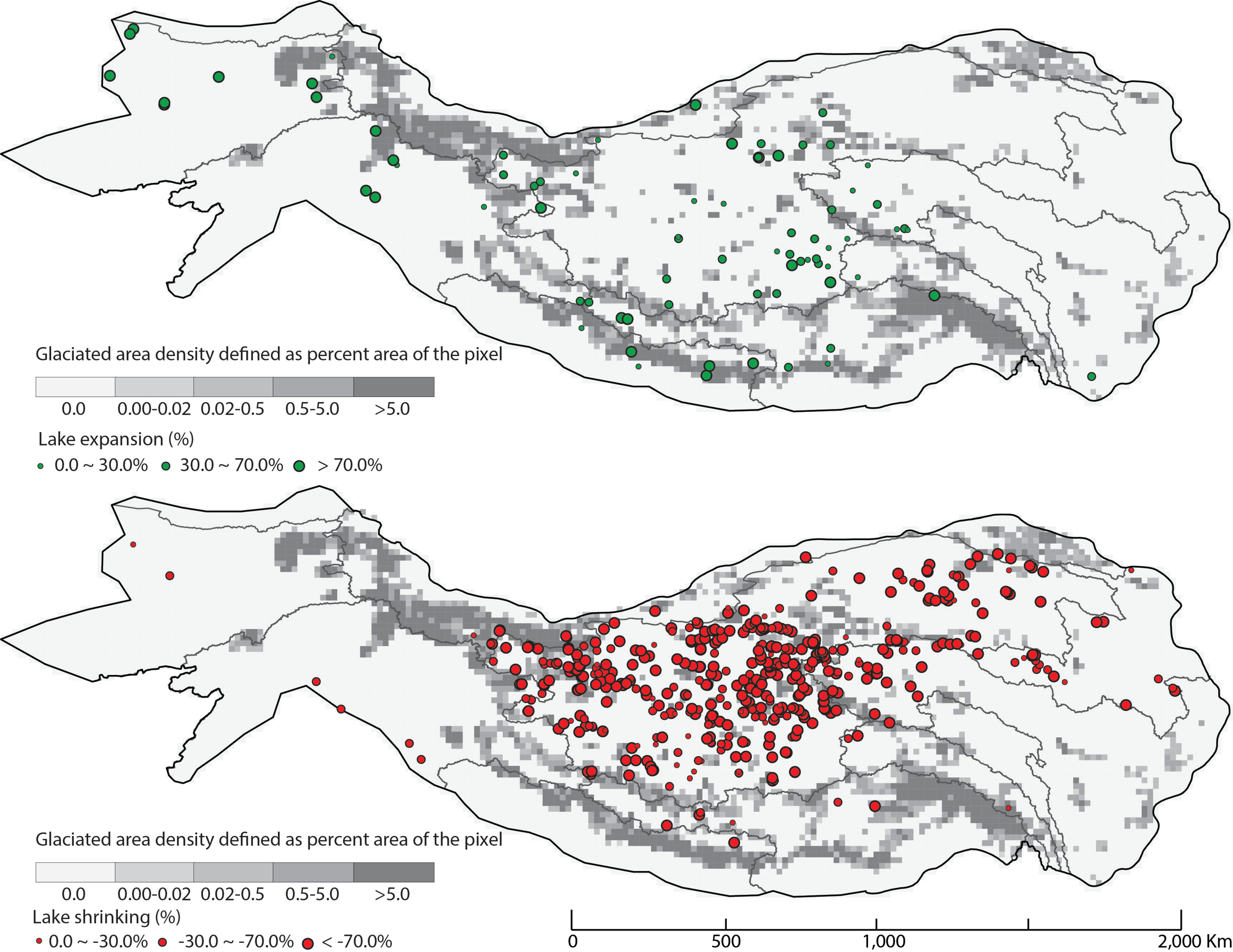
Figure 6.
Comparisons of lake fluctuations in lake shrinking period between the 1970s and 1995. The bottom figure shows that lake shrinking primarily occurred in the Himalayan Interior, Yangtze and Yellow basins, whereas lake expansions were often observed in the areas affected by the westerlies and glaciers (top figure).

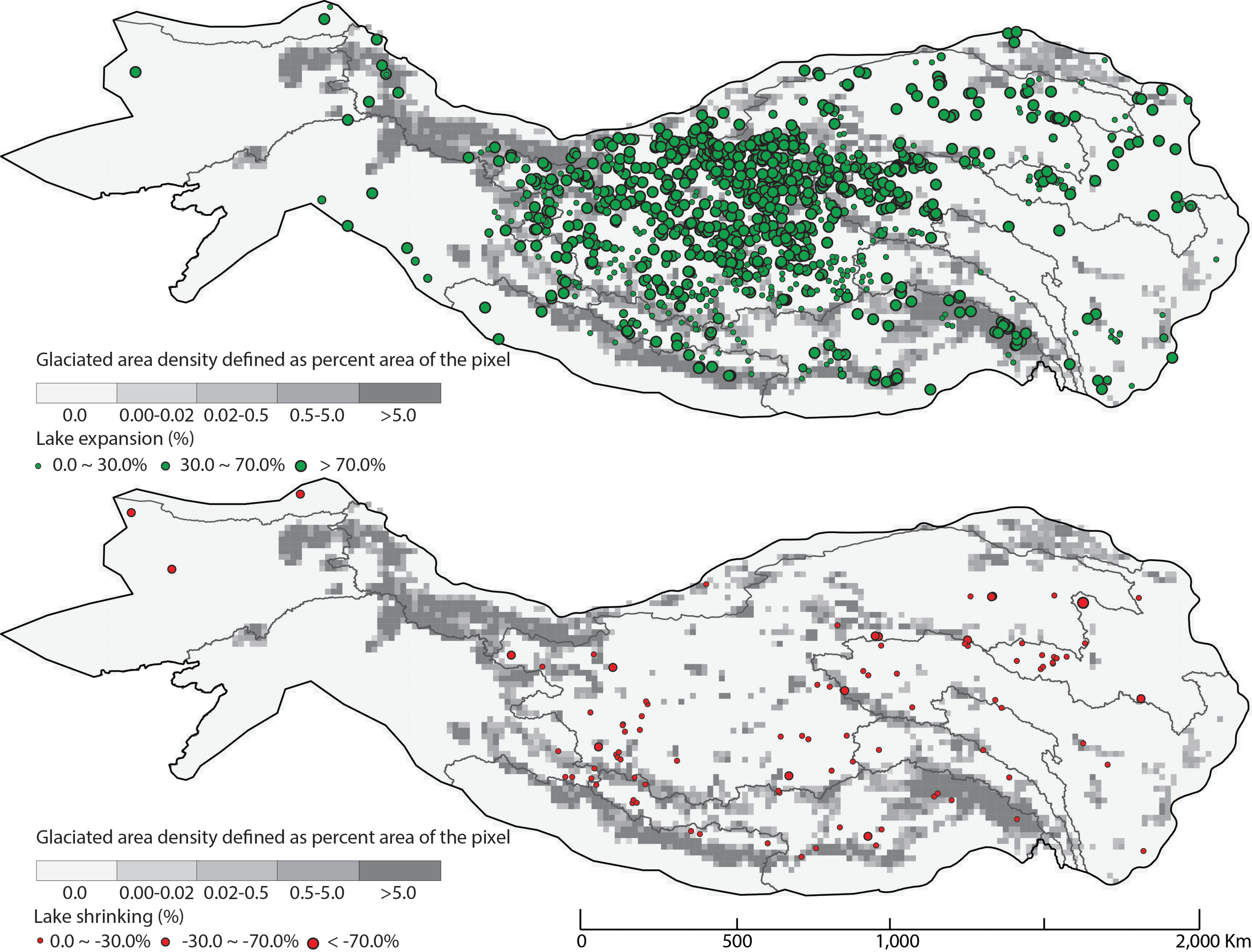
Figure 7.
Comparisons of lake fluctuations in lake expansion period between 1996 and 2015. The top figure shows that lake expansion is a common phenomenon in almost all the HKHT regions, and area decreasing for most of the shrunk lakes is not evident (bottom figure).
Figure 7.
Comparisons of lake fluctuations in lake expansion period between 1996 and 2015. The top figure shows that lake expansion is a common phenomenon in almost all the HKHT regions, and area decreasing for most of the shrunk lakes is not evident (bottom figure).

Figure 8.
Precipitation trend analysis using Mann-Kendall test in lake shrinking period from the 1970s to 1995 (the top figure), and lake expansion period from 1996 to 2015 (the bottom figure).
Figure 8.
Precipitation trend analysis using Mann-Kendall test in lake shrinking period from the 1970s to 1995 (the top figure), and lake expansion period from 1996 to 2015 (the bottom figure).

Figure 9.
The 100% stacked column charts of relative abundances of lakes in different elevation ranges and the line charts of year-by-year variations in average lake surface elevation in the HKHT Interior and the upper reaches of the nine Asian rivers.
Figure 9.
The 100% stacked column charts of relative abundances of lakes in different elevation ranges and the line charts of year-by-year variations in average lake surface elevation in the HKHT Interior and the upper reaches of the nine Asian rivers.

Figure 10.
Recent changes in relative glacier melt contribution (GMC) to lake water balance in the HKHT Interior and the upstream areas of the nine Asian rivers.
Figure 10.
Recent changes in relative glacier melt contribution (GMC) to lake water balance in the HKHT Interior and the upstream areas of the nine Asian rivers.

Figure 11.
Deviation area index (DAI) distribution against lake surface area delineated in high resolution images, which converges toward zero as the lake surface area increases.
Figure 11.
Deviation area index (DAI) distribution against lake surface area delineated in high resolution images, which converges toward zero as the lake surface area increases.

Figure 12.
Squared correlation coefficients () of predicting annual lake runoff for each of the ten river basins based on cross validation. Box plot shows the range of 25–75% quantiles for R2 distribution for each regression model.
Figure 12.
Squared correlation coefficients () of predicting annual lake runoff for each of the ten river basins based on cross validation. Box plot shows the range of 25–75% quantiles for R2 distribution for each regression model.


Table 1.
Summary of climatic, physical, and geomorphic information as well as data sources used in this study.
Table 1.
Summary of climatic, physical, and geomorphic information as well as data sources used in this study.
| Definition | Variable Name | Unit | Data Source |
|---|---|---|---|
| Climatic variables a | |||
| Mean annual precipitation Monthly precipitation | P P(Jan) | mm yr−1 mm yr−1 | Asian Precipitation—Highly-Resolved Observational Data Integration Towards Evaluation (APHRODITE) dataset [27] for 1975–2015. |
| Annual rainfall during monsoon season | PM | mm yr−1 | APHRODITE dataset for 1975–2015. |
| Mean annual land evapotranspiration | ET | inches yr−1 | Global Land Data Assimilation System product, GLDAS_NOAH025_M dataset (http://disc.sci.gsfc.nasa.gov/services/grads-gds/gldas) |
| Mean annual temperature | T | F° * 10 | APHRODITE dataset [27] for 1975–2015. |
| Mean max annual temperature | Tmax | F° * 10 | APHRODITE dataset [27] for 1975–2015. |
| Mean monthly temperature | T(Jan) | F° * 10 | APHRODITE dataset [27] for 1975–2015. |
| Mean max monthly temperature | Tmax(Jan) | F° * 10 | APHRODITE dataset [27] for 1975–2015. |
| Snow | Snow | cm | Annual snowfall, (APHRODITE) dataset [27] for 1975–2015. |
| Solar radiation | SR | mm yr−1 | GLDAS/Noah LSM Level 4 product (GLDAS_NOAH025_M) (http://disc.sci.gsfc.nasa.gov/services/grads-gds/gldas) |
| Soil moisture | SM | kg m−2 | GLDAS_NOAH025_M dataset (http://disc.sci.gsfc.nasa.gov/services/grads-gds/gldas) |
| Physical variables | |||
| Snow cover extent | SA | km2 | Image classification results, derived from Landsat images provided by the USGS Earth Resources Observation and Science (EROS) archive [28] |
| Bare land area | BA | km2 | Image classification results derived from Landsat images provided by EROS archive [28] |
| Meadowland area | MA | km2 | Image classification results derived from Landsat images provided by EROS archive [28] |
| River/stream surface area | WA | km2 | Image classification results derived from Landsat images provided by EROS archive [28] |
| Agricultural area (cropland) | AA | km2 | Image classification results derived from Landsat images provided by EROS archive [28] |
| Glaciered area | GA | km2 | GLIMS dataset [29] |
| GeomorphicVariables | |||
| Catchment area | CA | km2 | Derived from DEM data Shuttle Radar Topography Mission (SRTM) DEM data c [30] |
| Catchment relief | CR | m | Derived from SRTM DEM data [30] |
| Flow length | L | km | Derived from SRTM DEM data [30] |
| Mean catchment elevation | H | m | Derived from SRTM DEM data [30] |
| Average catchment slope | S | Degree | Derived from SRTM DEM data [30] |
| Drainage density | DD | km km−2 | Derived from SRTM DEM data [30] |
| Catchment wetness index b | CW | -- | Derived from SRTM DEM data [30] |
| Stream gradient | SG | m km−1 | Derived from SRTM DEM data [30] |
a Precipitation and temperature data were evaluated and calibrated using ground observations. Ground observations were obtained from two organizations, Global Historical Climatology Network (GHCN) and China Meteorological Administration (CMA). 572 ground observations, covering all the HKHT regions, were obtained from GHCN (https://www.ncdc.noaa.gov/data-access/land-based-station-data/land-based-datasets/global-historical-climatology-network-ghcn). Data from 184 meteorological stations in China were collected from CMA (http://cdc.cma.gov.cn/home.do). We then resampled the precipitation and temperature data to 1 km spatial resolution. The resampled data was calibrated with regard to vertical lapse rates [31].
b The variable is unitless.
c The 3 arc-second (~90 m) SRTM DEM data were void-filled, hydrologically conditioned, and resampled to create two DEM datasets with 0.25° and 1 km spatial resolution, respectively, as input datasets to calibrate precipitation and temperature data.
Table 2.
Summary of the recent changes in glacier runoff contribution to annual flow in the HKHT Interior and the upper reaches of nine large Asian rivers.
Table 2.
Summary of the recent changes in glacier runoff contribution to annual flow in the HKHT Interior and the upper reaches of nine large Asian rivers.
| River Basin Characteristics | GMC to Annual Lake Flow (%) | ||||||||
|---|---|---|---|---|---|---|---|---|---|
| Basin | Basin Area (km2) | Upstream Area (km2) | Annual Flow(m3/s) | No. of Glaciers | Glaciated Area (%) | 1975–1990 | 1991–2000 | 2001–2015 | |
| Affected by westerlies | Amu Darya | 534,739 | 393,558 | 2,123 | 7,804 | 1.7 | 27.0 | 26.5 | 33.3 |
| Indus | 1,081,718 | 499,244 | 5,533 | 10,867 | 2.6 | 19.5 | 17.3 | 24.6 | |
| Tarim | 1,152,448 | 303,410 | 146 | 11,732 | 5.7 | 34.2 | 37.0 | 38.1 | |
| Affected by ISM | Ganges | 1,016,124 | 235,940 | 18,691 | 6881 | 1.2 | 4.2 | 4.9 | 5.4 |
| Brahmaputra | 651,335 | 398,238 | 19,824 | 11,527 | 2.7 | 5.2 | 5.4 | 5.6 | |
| Salween | 271,914 | 108,070 | 1,494 | 2,100 | 1.5 | 3.6 | 4.2 | 4.4 | |
| Affected by EAM | Mekong | 805,604 | 83,959 | 11,048 | 393 | ~0.01 | 0.59 | 0.6 | 0.8 |
| Yangtze | 1,722,193 | 468,266 | 34,000 | 1,378 | 0.1 | 1.9 | 2.0 | 2.3 | |
| Yellow | 944,970 | 213,840 | 1,365 | 129 | ~0.02 | 0.3 | 0.4 | 0.4 | |
| HKHT Interior | 986,612 | 986,612 | n/a | 6,014 | 0.7 | 3.3 | 3.9 | 4.1 | |
Data source: World Resources Institute database [55]; International Center for Integrated Mountain Development (ICIMOD) technical report [56]; and Global Land Ice Measurements from Space (GLIMS) Glacier Database [29].
Note: The hydrological data may be different depending on the location of the gauging stations.
Table 3.
Regression models for the estimation of annual precipitation-induced runoff (Rp) using selected basin characteristics.
Table 3.
Regression models for the estimation of annual precipitation-induced runoff (Rp) using selected basin characteristics.
| Region | β0 | β1 | β2 | β3 | β4 | β5 | R2 |
|---|---|---|---|---|---|---|---|
| Amu Darya | — | CA 0.9861 | ET(June) −1.3177 | P(Jan) 1.5988 | P(July) 0.1885 | T −0.9632 | 0.6244 |
| Indus | 5.103 | CA 0.9967 | P 0.9945 | P(Jan) 0.7732 | Tmax −2.6723 | — | 0.6728 |
| Tarim | −25.761 | CA 0.8861 | P 2.2365 | CR 1.4141 | — | — | 0.6613 |
| Ganges | −11.7978 | CA 0.9571 | P(Nov) 0.7742 | S 0.5082 | P(Sept) 1.3205 | — | 0.6014 |
| Brahmaputra | −15.481 | CA 0.9908 | P 1.7739 | S 0.3527 | — | — | 0.6618 |
| Salween | 7.8715 | CA 0.9825 | Tmax −2.7132 | P(Aug) 0.8242 | P(May) 0.9432 | — | 0.4532 |
| Mekong | −27.761 | CA 0.8861 | P 2.2489 | H 1.1841 | — | — | 0.5119 |
| Yangtze | −9.855 | CA 0.9723 | P 2.0732 | ET −0.759 | Snow 0.0399 | P(July) 0.2156 | 0.7154 |
| Yellow | −6.088 | CA 0.9802 | P 1.9547 | T −1.1213 | — | — | 0.6234 |
| HKHT Interior | 3.559 | CA 0.9627 | P 1.7746 | Tmax(June) −2.4196 | — | — | 0.7428 |
© 2019 by the authors. Licensee MDPI, Basel, Switzerland. This article is an open access article distributed under the terms and conditions of the Creative Commons Attribution (CC BY) license (http://creativecommons.org/licenses/by/4.0/).
Share and Cite
MDPI and ACS Style
Yang, X.; Lu, X.; Park, E.; Tarolli, P. Impacts of Climate Change on Lake Fluctuations in the Hindu Kush-Himalaya-Tibetan Plateau. Remote Sens. 2019, 11, 1082. https://0-doi-org.brum.beds.ac.uk/10.3390/rs11091082
AMA Style
Yang X, Lu X, Park E, Tarolli P. Impacts of Climate Change on Lake Fluctuations in the Hindu Kush-Himalaya-Tibetan Plateau. Remote Sensing. 2019; 11(9):1082. https://0-doi-org.brum.beds.ac.uk/10.3390/rs11091082
Chicago/Turabian StyleYang, Xiankun, Xixi Lu, Edward Park, and Paolo Tarolli. 2019. "Impacts of Climate Change on Lake Fluctuations in the Hindu Kush-Himalaya-Tibetan Plateau" Remote Sensing 11, no. 9: 1082. https://0-doi-org.brum.beds.ac.uk/10.3390/rs11091082
Note that from the first issue of 2016, this journal uses article numbers instead of page numbers. See further details here.