Extending ALS-Based Mapping of Forest Attributes with Medium Resolution Satellite and Environmental Data

Abstract

Airborne laser scanner (ALS) data are used to map a range of forest inventory attributes at operational scales. However, when wall-to-wall ALS coverage is cost prohibitive or logistically challenging, alternative approaches are needed for forest mapping. We evaluated an indirect approach for extending ALS-based maps of forest attributes using medium resolution satellite and environmental data. First, we developed ALS-based models and predicted a suite of forest attributes for a 950 km² study area covered by wall-to-wall ALS data. Then, we used samples extracted from the ALS-based predictions to model and map these attributes with satellite and environmental data for an extended 5600 km² area with similar forest and ecological conditions. All attributes were predicted well with the ALS data (R² ≥ 0.83; RMSD% < 26). The satellite and environmental models developed using the ALS-based predictions resulted in increased correspondence between observed and predicted values by 13–49% and decreased prediction errors by 8–28% compared with models developed directly with the ground plots. Improvements were observed for both multiple regression and random forest models, and for the suite of forest attributes assessed. We concluded that the use of ALS-based predictions in this study improved the estimation of forest attributes beyond an approach linking ground plots directly to the satellite and environmental data.

1. Introduction

The increasing availability and decreasing cost of commercial airborne laser scanning (ALS) systems have resulted in widespread application of ALS data for enhancing forest inventories [1,2,3,4]. Forest attributes commonly predicted and mapped using ALS data include average tree height, density, mean diameter at breast height (DBH), gross total volume, gross merchantable volume, and biomass [5,6,7]. Most operational applications employ an area-based approach [8,9,10,11,12], whereby regression and other statistical techniques are used to relate metrics derived from the ALS data to attributes measured at ground sample plot locations [13,14,15]. The statistical models are then used to predict the attributes of interest at unsampled locations. The success of ALS data for predicting forest attributes has resulted in ALS data becoming a key data source for enhancing forest management inventories [16,17,18].

However, ALS data acquisition is not always possible for an entire area of interest due to limited resources or difficulties associated with covering remote or large areas. In such cases, alternative remote sensing data have been used to generate attribute predictions. For example, forest attributes have been linked directly to relatively inexpensive satellite data [19,20,21] using a variety of modeling methods (reviewed by Brofoske et al. [14]). Among the most common methods are regression [22,23,24], k-nearest neighbors (kNN) [25,26,27], and random forests [28]. Multispectral imagery such as Landsat Thematic Mapper (TM) [29,30] or Sentinel-2 (S2) [31] enhance the efficiency and cost effectiveness in mapping forest attributes over large forest landscapes. However, the use of multispectral imagery alone does not normally reach the level of accuracy possible with wall-to-wall ALS data [32].

Several studies have demonstrated the combined use of ALS data and satellite imagery to map forest attributes. Not surprisingly, models combining ALS with satellite variables generally provide better estimates than models using satellite imagery alone [32,33]. However, models using both ALS and satellite metrics can only be applied to areas that are sampled by ALS. One of the earliest studies to explore integration for the purpose of mapping locations unsampled by ALS was conducted by Hudak et al. [19]. These authors tested five aspatial and spatial methods for extending canopy heights and concluded that integration of ALS and Landsat data improved the utility of both datasets. Other studies have used ALS-derived estimates as a substitute for field plots and extended the ALS estimates with satellite imagery. For example, McInerney et al. [34] extended ALS-derived canopy heights using moderate resolution imagery from the Indian Remote Sensing satellite. Also focused on canopy height, Pascual et al. [35] developed multiple regression models between ALS-based height predictions and Landsat Enhanced Thematic Mapper (ETM+) band transformations and spectral indices for the purpose of extrapolating ALS height measurements across a broad landscape. Maselli et al. [36] evaluated both regression and kNN for extending stem volumes derived from mean stand heights obtained from ALS using Landsat ETM+ images. Subsequently, the concepts of “lidar plots” [37,38] and “lidar sampling” (reviewed by Wulder et al. [39]) were proposed to mitigate the need for extensive ground plot data for large-area forest characterization and mapping. In that context, Matasci et al. [40] used ALS plots and multitemporal Landsat composites to model cover, height, biomass, and other structural attributes for the entire boreal forest area of Canada. Although the spatial extent of that study is remarkable, the authors acknowledge that accuracy metrics reported in that study are to be interpreted with caution, as the ALS-predicted attribute values with variable accuracies were used as response variables.

The conceptual basis for a multilevel approach combining ground plots, ALS data, and satellite data for forest inventory is described in detail by Andersen et al. [41] and further demonstrated by others [42,43,44,45,46,47,48,49,50]. In a multilevel approach, relationships are first established between forest attribute values of ground plots and ALS data covering a portion of the area of interest. Then, relationships are established between samples extracted from the ALS data and spatial layers covering the entire area of interest. The multilevel approach thus allows estimation or map extension beyond the area covered by ALS using the spatially comprehensive layers. In Andersen et al. [41], implementation of the multilevel approach combining ground plots, ALS strip sampling, and satellite imagery provided total biomass estimates for the boreal forests of interior Alaska. Strunk et al. [42] demonstrated that the multilevel approach—referred to as an indirect approach—resulted in reduced estimates of residual variability for biomass by up to 36% relative to using Landsat imagery alone. Saarela et al. [43] reported relative standard errors in the range of 1–4% for model-assisted estimation of growing stock volume using multilevel sampling. Others have combined field, airborne, and spaceborne LiDAR (i.e., Geoscience Laser Altimeter System (GLAS) data) to produce regional maps of stand attributes [44] and to estimate aboveground biomass and carbon of boreal forests using multilevel sampling strategies [45,46,47,48,49,50]. Although these studies have demonstrated improved mapping and estimation capabilities using indirect or multilevel approaches, further evaluation is warranted with different data sets, at different scales, and for different forest conditions.

In this study, we hypothesized that the indirect approach including ALS samples would capture an extensive range of forest structure and environmental conditions, and thus improve prediction over a direct modeling approach that links a more limited set of ground plots to spatially comprehensive satellite and environmental data. We tested this hypothesis using parametric and nonparametric modeling methods commonly used for predicting forest attributes with ALS or satellite data, including multiple regression (e.g., [1,20,42]) and random forest (e.g., [51,52,53]). We developed ALS-based prediction models for a suite of forest attributes using ground plots and we predicted these attributes for a study area covered by wall-to-wall ALS data. Then, we used samples extracted from the ALS-based predictions to model forest attributes with multispectral, radar, and topographic data. We evaluated predictions from models developed using the ALS samples with those from models developed with only the ground plots using independent validation data. Finally, we produced maps of forest attributes for an extended area of boreal forest of western Newfoundland, Canada.

2. Materials and Methods

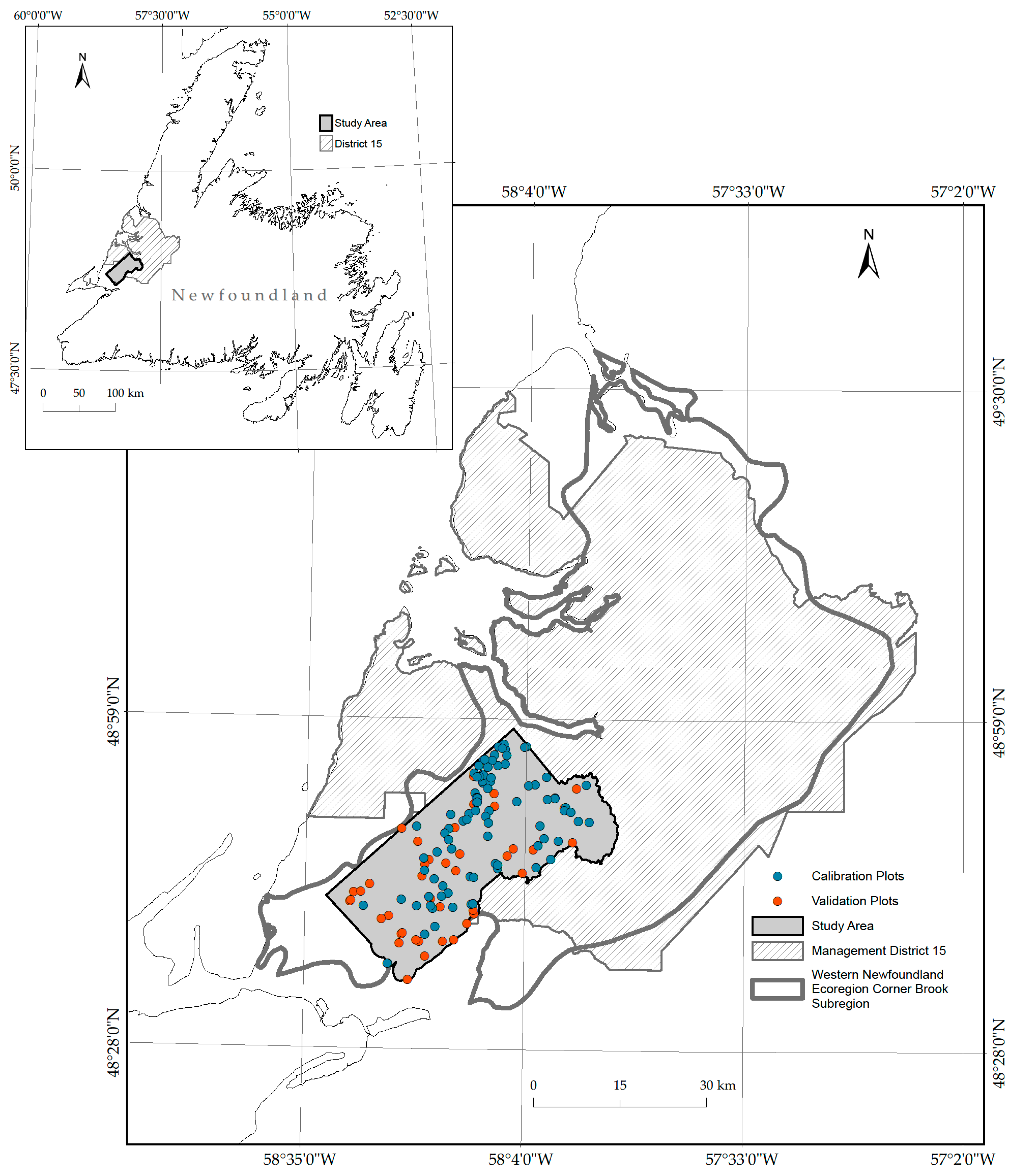
2.1. Geographic Area

Our geographic area of interest was Forest Management District 15, which covers an area of ~5600 km² centered around 49.04° N and 57.93° W, and corresponding closely with the Corner Brook Subregion of the Western Newfoundland Ecoregion (Figure 1). This ecoregion is located within the most eastern Boreal Forest Region of North America [54] and contains some of the most favorable sites for forest growth on the Island of Newfoundland [55]. Balsam fir (Abies balsamea (L.) Mill.)) is the dominant tree species of the region, and black spruce (Picea mariana (Mill.) Britton, Sterns & Poggenb.), white birch (Betula papyrifera Marsh.), yellow birch (Betula alleghaniensis Britton), and white spruce (Picea glauca (Moench) Voss) are also present. This region includes high productivity mountainous slopes underlain by orthic or gleyed podzols where seepage waters ensure good forest growth and profuse regeneration after cutting. In contrast, the region also includes the lower productivity coastal plain, dominated by coarse-textured deposits such as glacio-fluvial deposits, eskers, drumlins, and kames.

2.2. Ground Plots

We used two independent data sets of ground plots for calibrating and validating models of forest attributes. Both datasets were measured following ground sampling guidelines established for Canada’s National Forest Inventory [56]. The sample design aimed to capture the range of variability in the forest structure of the study area. For calibration, we selected potential sample locations using ALS data (described in Section 2.3) as a basis for stratification—following others who found improved accuracies using ALS-assisted plot selection for area-based inventory [57,58,59]. Instead of using specific ALS metrics (e.g., mean and standard deviation [58]), we performed a principal component analysis (PCA) [60] and represented forest structure by the first two components, which accounted for ~83% of the variance in ALS metrics. We used photo-interpreted forest inventory stand polygons to create stand-level dominant species masks and divided the range of values for each PCA component into 10 equal strata under each mask. We then selected a random sample location for ground-based assessment from each combination of species mask and PCA strata that existed within our study area. For validation, we selected potential sample locations using a stratified random sampling design using total volume predictions for conifer-dominated stands (result from Section 2.6) as the basis for stratification. We stratified the range of values of volume into 20 strata and randomly selected a minimum of two sample locations per strata.

We established circular plots with 11.28 m radius and recorded species, DBH (measured at 1.3 m), height, and status (live or dead) for all merchantable trees (trees ≥ 9 cm DBH). We recorded these same attributes for all trees with a minimum height of 1.3 m for a subplot of radius 3.99 m located in the center of each plot. We recorded the center location of each plot with a Trimble GeoExplorer, 6000 series XH global positioning system (GPS) with floodlight technology and used base station data to differentially correct the roving receiver data to within submeter accuracy. In total, we measured 89 calibration plots in 2016 and 2017, and 43 validations plots in 2018.

From the standard measurements of species, height, and DBH, we derived a suite of structural attributes for all plots. We calculated basal area of each tree from DBH. We estimated total and gross merchantable volumes as a function of DBH and height according to region- and species-specific equations from Warren and Meades [61,62]. We estimated above ground biomass (organic dry mass per unit area) with equations and coefficients published by Lambert et al. [63]. We used the individual attributes of live trees to estimate plot-level attributes including basal area weighted height (i.e., Lorey’s mean height) (HGT), basal area (BA), gross merchantable volume (GMV), total volume (TVOL), and aboveground biomass (B). We calculated attributes based on live trees (i.e., growing stock) for consistency with volume tables used by provincial and industrial agencies and because live-tree attributes are of interest for most operational and planning applications in the region. For the calculation of BA and GMV, we used only merchantable trees. With the exception of HGT, we converted values to per-hectare estimates. We also calculated species-specific basal areas as a percentage of the total BA of each plot and used these percentages to determine coniferous, broadleaf and mixed wood forest types.

We stratified the ground plots according to dominant forest type as is common practice for area-based modeling [60]. We labeled plots with ≥ 75% coniferous or broadleaf species as coniferous or broadleaf, respectively, and we labeled all other plots as mixed forest. For the current study, we focused on the coniferous forest, which represents ~90% of the productive forest of our study area and is the forest type of commercial importance to the region. Of the 89 calibration plots, 58 plots representing coniferous forest were used for calibration. Of the 43 validation plots, we removed four plots with GMV or TVOL that exceeded the range of the calibration data and were, therefore, not representative of the conditions modeled. This left 39 coniferous plots for validation and evaluation of our hypothesis (

Table 1. Descriptive statistics of forest attributes for ground plots.

Variable 1	Units	Calibration (n = 58)				Validation (n = 39)
		Min	Max	Mean	Std. Dev.	Min	Max	Mean	Std. Dev.
HGT	m	3.4	17.1	10.1	3.6	3.7	17.0	10.5	3.6
BA	m2 ha−1	0.4	63.2	30.1	18.1	0.9	62.7	33.8	16.5
GMV	m3 ha−1	0.8	401.5	156.9	118.7	1.7	376.8	175.2	109.5
TVOL	m3 ha−1	3.6	439.9	190.1	128.6	25.1	401.0	211.7	109.5
B	t ha−1	6.7	260.2	121.9	67.1	33.7	214.5	132.2	52.3

¹ HGT is Lorey’s height; BA is basal area; GMV is gross merchantable volume; TVOL is total volume; B is aboveground biomass.

).

2.3. ALS Data

Wall-to-wall ALS data were acquired between 15 August and 24 September 2016 representing an area of ~950 km² centered at 48.77° N and 58.19° W. The ALS data were acquired with a Riegl LMS-Q680i. The approximate flight altitude was 1000 m above ground level, with an approximate speed of 100 knots. The scan angle was ± 30° with 50% minimum overlap between flight lines. The aggregate pulse density was specified to be a minimum of six pulses m⁻². We calculated the resulting average point density to be 7.3 points m⁻² with a standard deviation of 2.4 points m⁻². Points were classified according to standard LAS specification classes [64] by the service provider.

We processed the ALS data to generate a digital terrain model (DTM) and a canopy height model (CHM) with spatial resolutions of 1 m × 1 m using the LTK^TM extension for ArcGIS [65]. For the DTM, we generated a triangular irregular network (TIN) using returns classified as ground and interpolated a raster surface from the TIN using natural neighbor interpolation. We used first returns classified as vegetation to generate the CHM, also using natural neighbor interpolation. We set the binning cell assignment to the maximum value, and replaced negative values with zeros.

We calculated metrics commonly used in forestry studies from normalized LiDAR point cloud data. The metrics consisted of height, structural, density, and cover statistics of each plot computed using LTK^TM [65]. We calculated all height, structural, and density metrics using vegetated returns ≥ 2 m representing treed vegetation [57] and ≤30 m to avoid erroneous points that exceeded that maximum tree height of the dominant trees species in the region [66]. Height metrics represented the basic statistics of mean (MEAN) and max (MAX) height and the heights of various percentiles of first returns (i.e., P10, …, P90, P95) [6]. Structural metrics were statistical measures of skewness (SKEW), coefficient of variation (COVAR), vertical distribution ratio (VDR) [67] and vertical complexity index (VCI) [68]. To compute density metrics, we divided the range of LiDAR heights into 10 equal intervals and calculated the cumulative proportion of LiDAR returns found in the first nine intervals (i.e., D1, …, D9) [6]. We calculated cover metrics at 2 m height intervals (i.e., CC2, …, CC14) from the CHM as the number of 1 m × 1 m cells with a height value > 2 m divided by the number of nonvoid 1 m × 1 m cells [53]. Finally, we selected a reduced set of metrics for this study avoiding very highly correlated predictor variables within each group (Pearson correlation coefficient, r > 0.95) (

Table 2. Description of airborne laser scanner (ALS), satellite and environment data used as predictor variables.

	Name	Units	Description
ALS Variables
Height Metrics 1	MAX	m	Maximum height of first returns
	P95	m	Height of the 95th percentile of first returns
	MEAN	m	Mean height of first returns
Structural Metrics 1	SKEW		Skewness of first returns
	COVAR		Standard deviation of first returns/mean of first returns
	VDR		Vertical distribution ratio [67]
	VCI		Vertical complexity index [68]
Density Metrics 1	D2	%	Percentage of all returns found in bins 1 through 2 of 10 where bin 2 represents the 20th percentile height of all returns
	D5	%	Percentage of all returns found in bins 1 through 5 of 10 where bin 5 represents the 50th percentile height of all returns
	D8	%	Percentage of all returns found in bins 1 through 8 of 10 where bin 8 represents the 80th percentile height of all returns
CHM Metrics	CC2	%	Number of 1 m × 1 m canopy height model cells that have a height value > 2 m divided by the number of nonvoid 1 m × 1 m cells
	CC6	%	Number of 1 m × 1 m canopy height model cells that have a height value > 6m divided by the number of nonvoid 1 m × 1 m cells
	CC14	%	Number of 1 m × 1 m canopy height model cells that have a height value > 14m divided by the number of nonvoid 1 m × 1 m cells
Satellite Variables
Sentinel 2 2	S2_B2	%	Blue band; original resolution 10 m
	S2_B4	%	Red band; original resolution 10 m
	S2_B5	%	Vegetation red edge; resolution 20 m
	S2_B8	%	NIR; original resolution 10 m
	S2_B11	%	SWIR; resolution 20 m
PALSAR	HH	DN	Radar backscatter — HH polarization; original resolution 25 m
	HV	DN	Radar backscatter — HV polarization; original resolution 25 m
Environmental Variables
Topographic and Solar Radiation	Elevation	m	Elevation above mean sea level from 0.75 arc second CDEM [69]
	CosAspect	−1 to 1	cos(Aspect) transformation representing northness
	SCOSA		Slope × cos(Aspect) transformation [70]
	SINA		Slope × sin(Aspect) transformation [70]

¹ Metrics computed from returns classified as vegetation with heights ≥ 2 m and ≤ 30 m. ² Pixel radiometric measurements are Level1C Top of Atmosphere (TOA) reflectances.

).

2.4. Spatially Comprehensive Data

We used spectral, structural, and topographic data that were readily available and spatially comprehensive for our area of interest. For the spectral data, we mosaicked four Level-1C orthorectified Sentinel-2 (S2) images [71] acquired on 27 June 2017 under virtually clear skies. The S2 images consisted of 13 spectral bands; however, bands 1, 9, and 10 were not used in this study due to their coarse resolution (60 m × 60 m), and bands 3, 7, 8A, and 12 were omitted to minimize redundancy with other bands (Pearson correlation coefficient, r > 0.95). We resampled bands with an original spatial resolution of 10 m × 10 m to 20 m × 20 m prior to mosaicking. Similarly, we resampled Advanced Land Observing Satellite (ALOS) Phased Arrayed L-band Synthetic Aperture Radar (PALSAR) HH and HV polarization mosaic data available at 25 m × 25 m spatial resolution [72] and Canadian Digital Elevation Model (CDEM) raster data [69] with a base resolution of 0.75 arc seconds (~23 m) in the north–south direction to 20 m × 20 m. We generated solar radiation transformations including CosAspect, SCOSA, and SINA [70] by combining slope and aspect information derived from the CDEM.

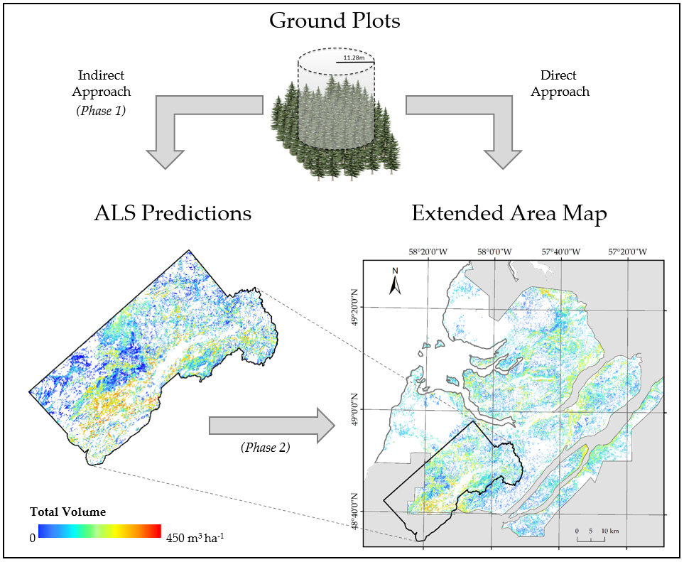
2.5. Overview of the Approach

Our implementation of the indirect mapping approach consisted of two phases with an independent evaluation. In the first phase, we built predictive models between the calibration plot attributes and ALS plot metrics. For the second phase, we built predictive models between ALS-based predictions and variables derived from the spatially comprehensive satellite and environmental data. For comparative purposes, we also built predictive models directly between the calibration plot attributes and the satellite and environmental variables. In all cases, we developed both random forest and multiple linear regression models and we evaluated model goodness-of-fit by regressing observed vs. predicted values for independently measured validation plots [73,74]. We produced maps by applying the predictive models to 20 m × 20 m raster grids.

2.6. Development of ALS-Based Inventory (Phase 1)

In phase 1, we built random forest models [75] in R [76] with ModelMap [77]. ModelMap automates the process of model building and map construction by providing an interface with several R packages, including randomForest [78]. Each random forest model consisted of 500 trees by default whereby each tree was developed with a random subset of the reference data and a random selection of predictors at each node of the tree to determine the split. We assessed variable importance during initial model development and retained only those predictors with a %IncMSE greater than 3% for the final models. We used tuneRF to determine the optimal number of predictor variables to retain at each node (mtry) for each model. The tuneRF algorithm starts with a default value of mtry (i.e., the number of predictors divided by three) and searches for the optimal value according to out-of-bag error estimates. The optimal values of mtry varied depending on the attribute modeled. During model development, we evaluated the random forest models according to out-of-bag errors.

We developed regression models using a subset regression technique available in the R package Leaps [79]. Leaps exhaustively searches all pathways to choose the best variable subsets for a given number of predictors. For each response variable, we used Leaps to identify the 10 best models for each combination of predictors according to the method of Mallows’ Cp [80], where the Cp statistic is an indicator of balance between models that are too simple and may suffer from biased coefficients and biased prediction, or too complicated, resulting in large variances in both the coefficients and the prediction [81]. We used statistical tests to determine whether each model met the assumptions of linear regression, including the Shapiro–Wilk Test for normality of residuals [82] and the Breusch–Pagan Test for homogeneity of variance [83]. Variance inflation factors (VIF) identified problems with collinearity [81]. We removed models from the candidate set where model tests indicated heteroscedasticity, non-normality of residuals (p < 0.05) or collinearity (VIF ≥ 7). Of the remaining models, we selected the model with the lowest Akaike’s information criterion (AIC) [84] score. During model development, we assessed the regression models using leave-one-out cross validation.

We generated raster grids for each predictor variable at 20 m × 20 m spatial resolution for the ALS site, and we used the models to predict the response variable for each raster cell. We implemented the random forest models using the R package ModelMap [77] and the regression models using the R package raster [85].

2.7. Development of Extended Inventory (Phase 2)

The ALS-based raster products from phase 1 provided more than two million potential samples (i.e., raster cells) for calibrating the satellite and environmental models. We converted the raster cells to a points shape file using ESRI ArcGIS [86] and we input the points shape file in R [76], where we filtered the potential samples to provide calibration data that were representative of the relevant forest conditions as follows. First, we assumed—due to our sampling design—that our ground plots represented the range of forest conditions of interest to this study. Therefore, we removed potential samples that had ALS metric values outside the range of those observed at the ground plots (e.g., MAX < 3.44 m & > 21.54 m). We also removed potential samples located in areas of cloud or cloud shadow and areas harvested on the satellite imagery since the time of ALS acquisition. To do this, we established thresholds for band 2 (> 0.7 & < 0.09), 3 (> 0.6 & < 0.11) and 4 (> 0.03 & < 0.08) by visually assessing the imagery. Finally, we removed samples from areas with ≤ 75% coniferous forest according to a recent forest management inventory of the area as models only represented the coniferous forest. After filtering, 828,853 potential samples remained. We subsampled the remaining samples by dividing the range of the predicted response variable into 10 equal strata and randomly selected 500 samples within each strata for a total of 5000 samples for each attribute of interest. We used the R package BalancedSampling [87] and the Spatially Balanced Local Pivotal Method [88,89] to select samples that were spatially, spectrally, structurally, and topographically representative of the forest conditions within each strata. We balanced the samples spatially on longitude and latitude, spectrally on S2 band 4 reflectance values, structurally on the PALSAR HV polarization radar backscatter, and topographically on elevation. Using the resulting samples as calibration data sets, we developed random forest and regression models using the same methods as applied in phase 1. We assessed out-of-bag errors (random forest) and leave-one-out cross validation results (regression) to evaluate the quality of the phase 2 models for capturing the relationship between the ALS predictions of forest attributes and the satellite and environmental predictor variables.

2.8. Independent Plot Evaluation

We evaluated the indirect modeling approach relative to the direct modeling approach using the independent validation plots and common measures used to evaluate area-based model performance [60,74]. Evaluation statistics included: correspondences between observed and predicted values as indicated by the coefficient of determination (R²), the root mean square deviation (RMSD Equation (1)), relative root mean square deviation expressed as a percentage of the mean (RMSD%, Equation (2)), absolute measure of model bias, (Bias, Equation (3)), and relative bias expressed as a percentage of the mean (Bias%, Equation (4)):

$$\mathrm{RMSD}=\sqrt{\frac{{{\displaystyle \sum }}_{i=1}^n{\left(y_i-{\widehat{y}}_i\right)}^2}{n-1}}$$

(1)

$$\mathrm{RMSD}\%=\frac{\mathrm{RMSD}}{\overline{y}}\times 100$$

(2)

$$\mathrm{Bias}=\frac{{{\displaystyle \sum }}_{i=1}^n\left(y_i-{\widehat{y}}_i\right)}{n}$$

(3)

$$\mathrm{Bias}\%=\frac{\mathrm{Bias}}{\overline{y}}\times 100$$

(4)

where y_i is the observed value, ŷ_i is the predicted value for case i, and n is the number of observations. The absolute RMSD and Bias provide error estimates in the units of the respective forest attributes, whereas the relative RMSD and Bias allow for comparisons between different forest attributes.

We repeated the direct and indirect approaches with five random seeds whereby the seeds influenced the selection of samples and predictors for the random forest models and the selection of spatially balanced samples in phase 2 for both the random forest and regression models. We implemented the Vuong test [90] with the R package nonnest2 [91] to determine significant differences between the results of the direct and indirect approaches and between the random forest and regression methods.

3. Results

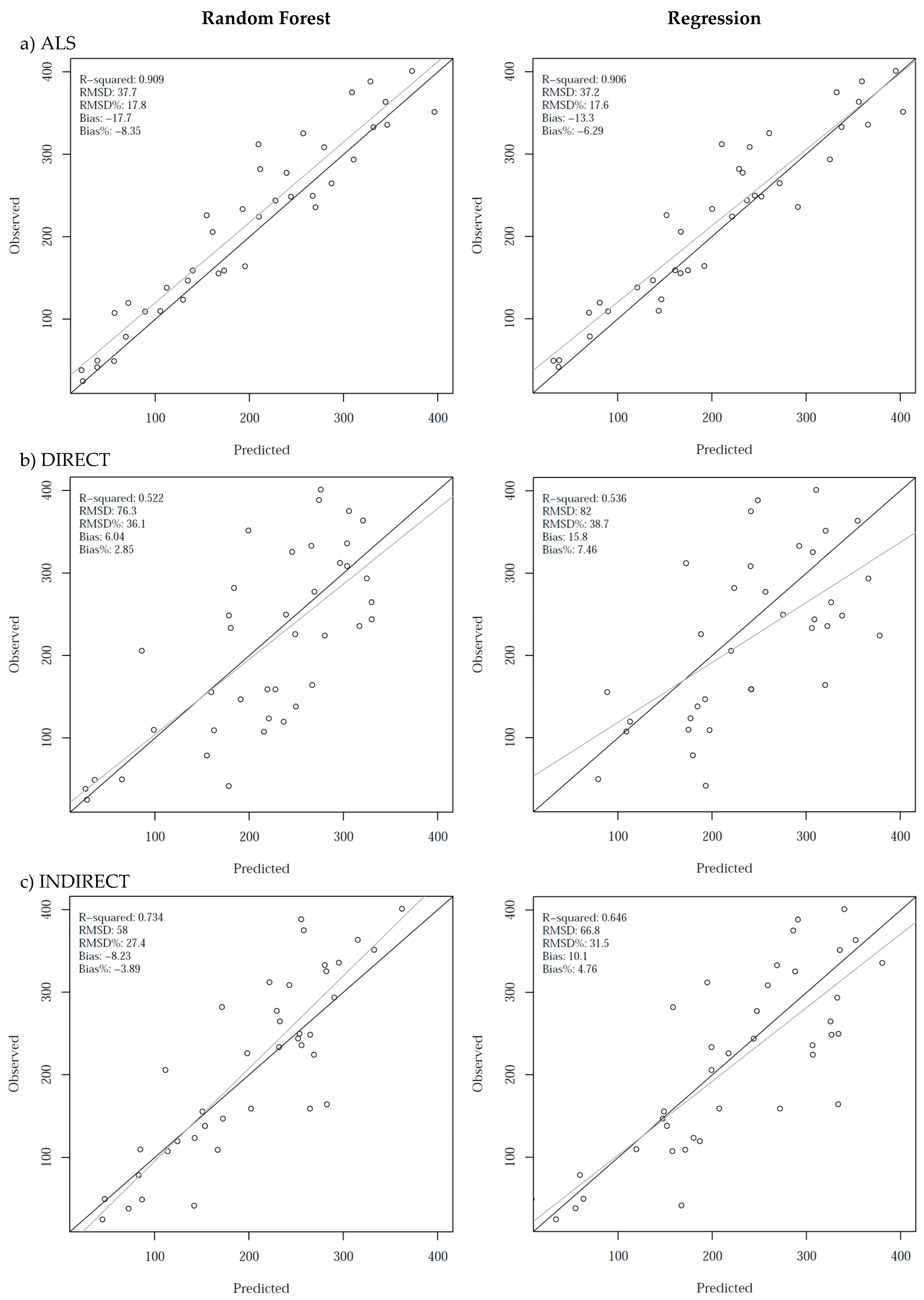
3.1. ALS Models of Forest Attributes (Phase 1)

The phase 1 models developed with ALS predictors resulted in high correspondence between predicted and observed values for both the calibration (R² > 0.90) and validation data sets (R² > 0.83) (

Table 3. Evaluation statistics for ALS-based prediction of forest attributes ¹.

	Random Forest					Regression
	R2	RMSD	RMSD%	Bias	Bias%	R2	RMSD	RMSD%	Bias	Bias%
Calibration 2 (n = 58)
HGT	0.93	0.95	9.37	0.09	0.84	0.95	0.84	8.27	0.00	0.00
BA	0.90	5.67	18.86	0.08	0.28	0.92	5.22	17.37	0.00	0.00
GMV	0.94	29.11	18.56	1.35	0.86	0.94	30.31	19.33	0.00	0.00
TVOL	0.94	31.29	16.46	0.04	0.02	0.96	27.72	14.58	0.00	0.00
B	0.90	21.49	17.63	0.43	0.35	0.93	18.74	15.37	0.00	0.00
Validation (n = 39)
HGT	0.94	1.14	10.86	−0.53	−5.09	0.95	1.03	9.79	−0.54	−5.17
BA	0.83	7.56	22.40	−3.03	−8.97	0.86	6.71	19.87	−2.44	−7.23
GMV	0.88	44.76	25.55	−22.19	−12.67	0.90	40.07	22.87	−18.40	−10.50
TVOL	0.91	37.84	17.87	−17.03	−8.04	0.91	37.21	17.57	−13.32	−6.29
B	0.85	22.14	16.75	−5.86	−4.43	0.83	23.71	17.93	−4.28	−3.24

¹ Random forest values represent average results of five random seeds. ² Calibration results are calculated from out-of-bag samples for random forest and leave-one-out cross validation for regression.

). Prediction errors were low for the calibration set (RMSD% < 20; Bias% < 0.9) but slightly higher for the validation set (RMSD% < 26; Bias% < 13), as we would expect. Observed versus predicted scatter plots showed most plots near the 1:1 line (e.g., TVOL, Figure 2a; other attributes not shown). Overall, the evaluation statistics indicated strong prediction models for all attributes reported. Moreover, differences in the error statistics for the random forest and regression models were minimal (R² < 0.03; RMSD% < 3; Bias% < 3). Therefore, we deemed the ALS-based predictions from both the random forest and regression models as suitable for use as calibration data for phase 2.

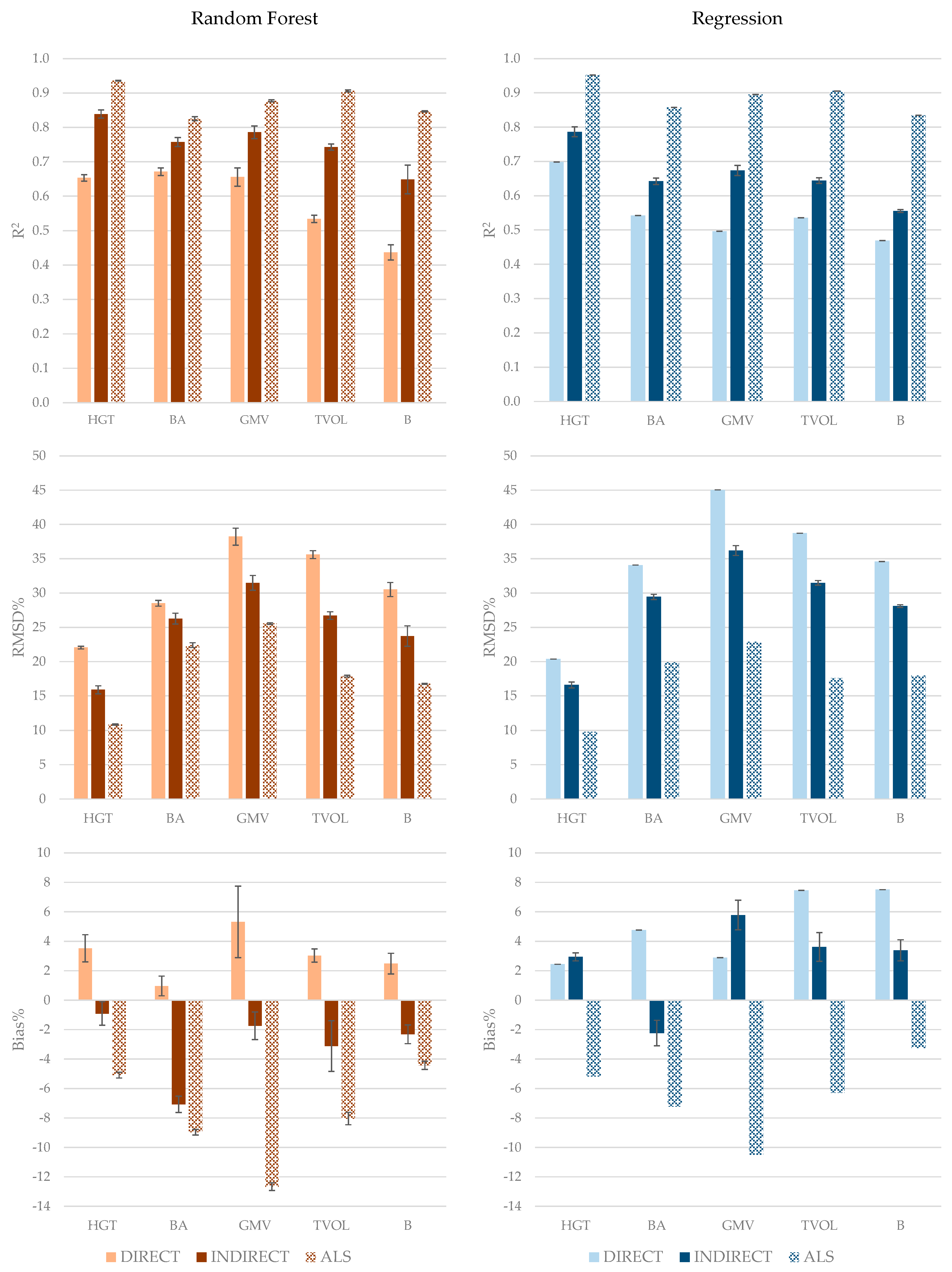
3.2. Satellite and Environmental Models (Phase 2)

The phase 2 models with satellite and environmental predictors had moderate correspondence between predicted and observed values for the calibration (R² = 0.58–0.74) and validation (R² = 0.56–0.84) data sets (

Table 4. Evaluation statistics for prediction of forest attributes with satellite and environmental variables ¹.

	Random Forest					Regression
	R2	RMSD	RMSD%	Bias	Bias%	R2	RMSD	RMSD%	Bias	Bias%
Calibration 2 (n = 5000)
HGT	0.71	1.81	17.85	0.01	0.09	0.68	2.17	21.16	0.00	0.00
BA	0.70	8.14	27.11	0.04	0.14	0.66	9.80	32.20	0.00	0.00
GMV	0.67	59.40	31.66	0.50	0.26	0.58	73.06	36.49	0.00	0.00
TVOL	0.70	61.64	28.30	0.14	0.06	0.61	76.73	34.73	0.00	0.00
B	0.74	30.43	23.31	0.21	0.16	0.67	39.43	30.63	0.00	0.00
Validation (n = 39)
HGT	0.84	1.66	15.88	−0.09	−0.91	0.79	1.74	16.59	0.31	2.94
BA	0.76	8.87	26.27	−2.39	−7.08	0.64	9.93	29.43	−0.75	−2.24
GMV	0.79	55.14	31.47	−3.04	−1.74	0.67	63.41	36.20	10.13	5.78
TVOL	0.74	56.55	26.71	−6.60	−3.11	0.64	66.66	31.48	7.64	3.61
B	0.65	31.36	23.72	−3.07	−2.32	0.56	37.15	28.10	4.47	3.38

¹ Random forest values represent average results of five random seeds. ² Calibration statistics are calculated from out-of-bag samples for random forest and leave-one-out cross validation for regression.

). However, in this case, the random forest models consistently outperformed the regression models, with R² values increasing by 4–9% based on the calibration data and by 5–12% based on the independent validation data. Similarly, RMSD% values decreased for all attributes by 1–7%. These results suggest that the random forest models may better capture the complex relationship between the forest attributes and the satellite and environment variables, compared with the more simple regression models. Bias was low in all cases (Bias% < 8%). Surprisingly, the error statistics of the independent validation results were not markedly poorer than those of the calibration data sets assessed via out-of-bag samples for random forest and using leave-one-out cross validation for regression. These results further suggest that the ALS predictions provided suitable calibration data for developing the satellite and environmental models.

3.3. Direct vs. Indirect Approach

For all attributes studied, the indirect approach resulted in higher correspondence between observed and predicted values than the direct approach (e.g., TVOL, Figure 2b and c; Figure 3). R² values increased by 13–49% for random forest and 13–36% for regression depending on the attribute. Similarly, mean deviation of predicted values with respect to the observed ones was consistently lower for the indirect approach than the direct approach by 8–28% for random forest and 14–20% for regression. These error statistics favor the indirect approach over the direct approach—when using the satellite and environmental models to map the extended area. Not surprising, the ALS-based predictions had the most favorable error statistics overall, with the exception of bias. Bias was negative for all attributes for the ALS-based predictions, but more variable for the direct and indirect approaches. However, bias was less than 13% for all attributes regardless of the approach used.

Although the ALS models predicted all attributes well (R² > 0.83, Table 3), HGT had the most favorable error statistics for the satellite and environmental models (Figure 3). Better results were achieved for the indirect approach (R² > 0.79; RMSD% < 17^; Bias% < 3), whereas the results of the direct approach were poorer (R² < 0.70; RMSD% > 20; Bias% < 4) for both random forest and regression models. The attribute with the least favorable results based on the satellite and environmental variables was GMV. Again, the results of the indirect approach (R² > 0.67; RMSD% < 37; Bias% < 6) were more favorable than those of the direct approach (R² < 0.66; RMSD% > 38; Bias% < 6).

For illustration, we present observed versus predicted scatter plots for TVOL for each approach based on the independent validation data (Figure 2). The results represent a single seed, however, the scatter plots and associated statistics were similar regardless of the seed selected (results not shown). The correspondence between the observed and ALS-based predictions was strong (R² > 0.90; RMSD% < 18) for both random forest and regression (Figure 2a). Not surprisingly, the predictions from the satellite and environmental variables showed weaker correspondence with higher prediction errors than those achieved with ALS. However, the indirect approach (Figure 2c) provided more favorable results than the direct approach (Figure 2b) for random forest (R² = 0.73 vs. 52; RMSD = 58 vs. 76.3 m³ ha⁻¹) with the exception of bias, which increased and switched from positive to negative (Bias = −8.23 vs. 6.06 m³ ha⁻¹). For regression, the indirect approach provided more favorable results for all three error statistics (R² = 0.65 vs. 0.54; RMSD = 66.8 vs. 82 m³ ha⁻¹; Bias = 10.1 vs. 15.8 m³ ha⁻¹).

Vuong tests indicated that the differences in the relationship between observed and predicted values between the direct and indirect approaches were statistically significant (P_DIFF < 0.05) for all attributes. Moreover, there was sufficient evidence that the indirect approach performed better than the direct approach (P_INDvsDIR < 0.05) for all attributes except BA for random forest (P_INDvsDIR = 0.05) and B for regression (P_INDvsDIR = 0.10) (

Table 5. Vuong test comparing observed versus predicted values from (a) the direct and indirect approaches and (b) random forest and regression models.

(a) Direct vs. Indirect
	Random Forest					Regression
	R2DIR	R2IND	pDIFF	pDIRvsIND	pINDvsDIR	R2DIR	R2IND	pDIFF	pDIRvsIND	pIND vsDIR
HGT	0.67	0.86	0.000	0.999	0.001	0.70	0.79	0.001	0.996	0.004
BA	0.68	0.77	0.000	0.947	0.053	0.54	0.65	0.000	0.982	0.018
GMV	0.67	0.80	0.000	0.977	0.023	0.50	0.68	0.000	1.000	0.000
TVOL	0.54	0.76	0.000	0.993	0.007	0.54	0.65	0.000	0.960	0.040
B	0.44	0.66	0.000	0.991	0.009	0.47	0.56	0.000	0.895	0.105
(b) Random Forest vs. Regression
	Direct					Indirect
	R2RF	R2REG	pDIFF	pRFvsREG	pREGvsRF	R2RF	R2REG	pDIFF	pRFvsREG	pREGvsRF
HGT	0.67	0.70	0.000	0.626	0.374	0.86	0.79	0.000	0.025	0.975
BA	0.68	0.54	0.000	0.060	0.940	0.77	0.65	0.000	0.000	1.000
GMV	0.67	0.50	0.000	0.018	0.982	0.80	0.68	0.000	0.004	0.996
TVOL	0.54	0.54	0.000	0.491	0.509	0.76	0.65	0.000	0.002	0.998
B	0.44	0.47	0.000	0.617	0.383	0.66	0.56	0.000	0.008	0.992

p_DIFF: variance test if the models are significantly different; p_DIRvsIND: likelihood ratio test that the direct (DIR) model fits better than the indirect (IND) model; p_INDvsDIR: likelihood ratio test that the indirect (IND) model fits better than the direct (DIR) model; p_RFvsREG: likelihood ratio test that the random forest (RF) model fits better than the regression (REG) model; p_REGvsRF: likelihood ratio test that the regression (REG) model fits better than the random forest (RF) model.

a). Vuong tests comparing the relationships between observed and predicted values for random forest and regression suggest sufficient evidence that the random forest models performed better than the regression results for the indirect approach (P_RFvsREG < 0.05) and for the direct approach for GMV (P_RFvsREG = 0.02), but not so for the direct approach and the remaining forest attributes (P_RFvsREG > 0.05₎ (Table 5b).

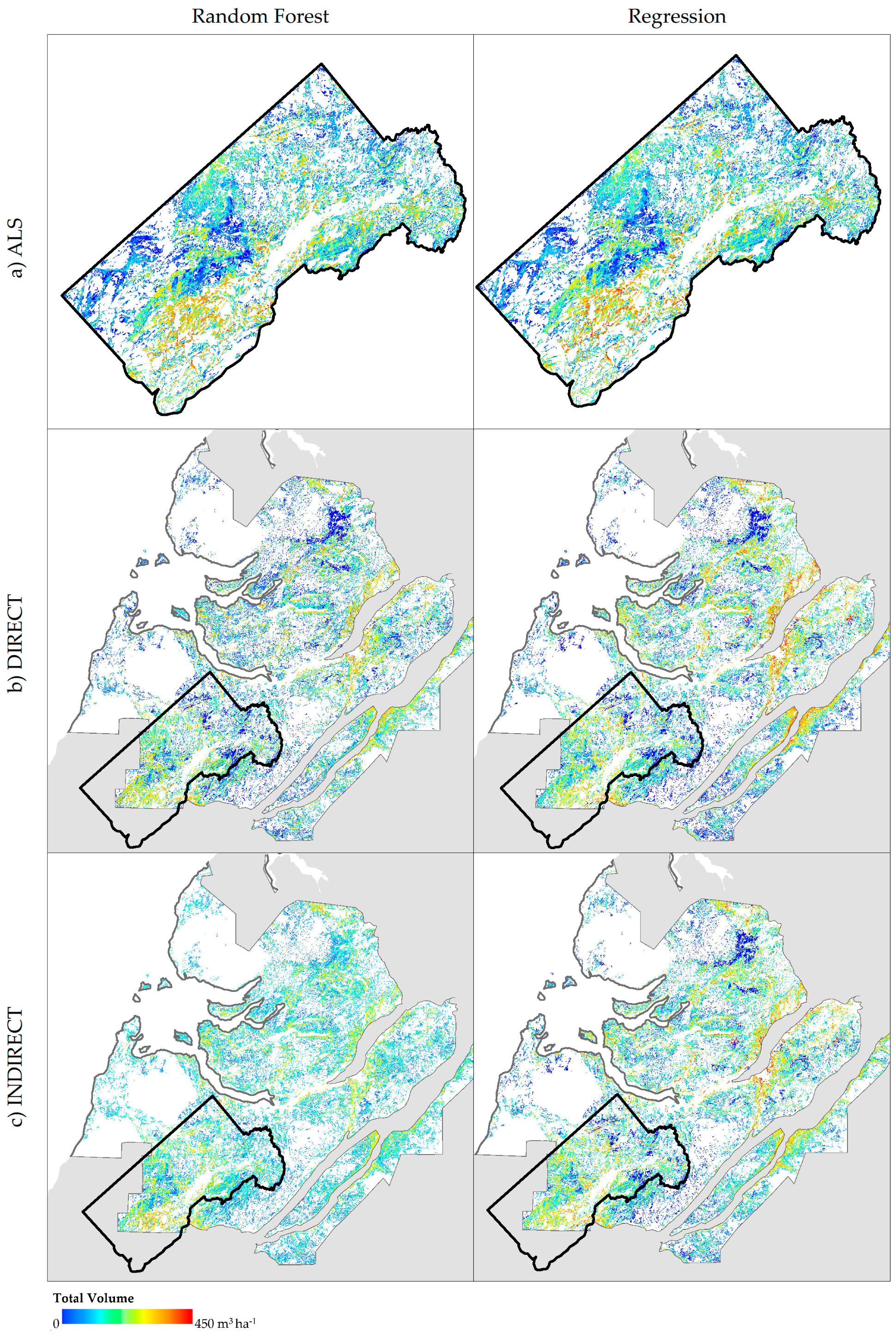
3.4. Landscape Patterns

Maps illustrate landscape patterns of the attribute predictions (e.g., TVOL, Figure 4). The phase 1 maps of the study site generated with ALS metrics are visually similar regardless of the modeling method used. This observation is consistent with the fact that both the random forest and regression models were strong with low prediction errors. The maps generated with the satellite and environmental variables exhibit greater variation between the direct and indirect approaches and between the random forest and regression models. Based on the independent evaluation, the optimal results were achieved for the indirect approach over the direct approach and for the random forest models over the regression models. The map of TVOL produced with the indirect approach and the random forest models showed the greatest similarity with the ALS predictions. There appears to be a slight overestimation of the low volume areas and a slight underestimation of high volume areas, as is also evident from the scatter plots (Figure 2c) and in the more limited range of values mapped with the random forest models. The maps from the direct approach and from the regression models had more low values (TVOL < 50 m³ ha⁻¹) and more high values (TVOL > 400 m³ ha⁻¹) throughout the ALS area and the extended district. These map observations are consistent with the slight underestimation of the low volume plots and overestimation of the high volume plots observed in the corresponding scatter plots of Figure 2.

4. Discussion

4.1. ALS-Based Inventory

We generated a suite of ALS-based models for predicting attributes of conifer-dominated forests of western Newfoundland, Canada. All models had R² values of 0.83 or greater and relative RMSD values < 26% of mean values based on independent validation data. The model prediction errors and mapped products were similar using both regression and random forest models. These results are consistent with many other studies demonstrating the use of ALS for area-based estimation of forest attributes in boreal forest conditions [1,6,7,53]. However, in many instances, wall-to-wall ALS coverage is not available. Therefore, we evaluated the use of a subarea of ALS coverage to calibrate satellite and environmental data that offers spatially comprehensive coverage over an extended area.

4.2. Extension of ALS-Based Inventory

The approach used in this study combines information measured at ground plots with a subarea of wall-to-wall ALS data and spatially comprehensive satellite and environmental data to map forest attributes for an extended area of interest. More specifically, we used ALS-based predictions to provide thematic and spatial balance, a highly desirable property of area-based inventory design. We used S2 spectral bands and PALSAR L-band SAR backscatter combined with topographic and solar radiation variables to provide complementary information for extending the ALS-based inventory over an area with similar ecological conditions. The ALS-based predictions improved representation of the range of forest and environmental conditions available for calibrating the spatially comprehensive data in an indirect estimation and mapping approach.

The practical justification for such an approach requires demonstration that the prediction of inventory attributes exceeds that achieved by linking ground plots directly to spatially comprehensive satellite and environmental data [42]. Accordingly, we tested the hypothesis that the indirect modeling approach using ALS-based predictions as calibration data improves prediction over a direct modeling approach using a more limited set of ground plots. In evaluating the hypothesis, we used an independent set of ground plots measured within two years of the ALS and satellite data acquisitions. Improvements in R² and RMSD were observed for the indirect approach over the direct approach for all attributes analysed in this study. The satellite and environmental models developed using the ALS-based predictions resulted in increased correspondence between observed and predicted values by 13–49% and decreased prediction errors by 8–28% compared with models developed directly with the ground plots. Significance tests suggested that there was sufficient evidence that the indirect approach was better than the direct approach for four of the five attributes regardless of whether random forest or regression models were used. Thus, the evaluation with independent validation plots confirmed our hypothesis for several key forest attributes of western Newfoundland boreal forests. This finding is important because the added cost of ALS data acquisition for a portion of an area of interest can be justified if the prediction accuracy exceeds an approach using only the ground plots.

4.3. Parametric vs. Nonparametric Models

Random forest (nonparametric) and regression (parametric) models have advantages and disadvantages when it comes to operational prediction of forest inventory attributes [53]. Random forest models take full advantage of the data set and do not require prior specification. As random forest models never predict outside the range of the data, there are no concerns with extreme predictions, but regression allows for model fitting with more limited data. However, there are additional considerations when developing regression models as regression models must satisfy conditions of normality, heterogeneity, significance of predictors, and collinearity. Furthermore, the number of possible predictors is limited by the sample size to avoid overfitting.

Our results suggest that both random forest and regression models were suitable for predicting forest inventory attributes from ALS data. In our study, the differences between the random forest and regression model predictions with ALS metrics were not significant. Similarly, for the direct approach, we did not find sufficient evidence that the random forest models fit better than the regression models, with the exception of GMV. On the contrary, the indirect approach implemented with random forest models resulted in better correspondence between predicted and observed values and reduced prediction errors relative to the direct approach. This may be in part due to the ability of random forest models to capture the more complicated relationships between forest attributes and the satellite and environmental data, whereas the regression models are based on the linear relation hypothesis.

4.4. Data and Technical Considerations

The results of this study are likely dependent upon the quality of the remote sensing data sets used. For phase 1, we acquired ALS data with parameters optimized for forest applications [92] including 50% overlap between flight lines with minimum aggregate pulse densities of six points per square meter. Single-pass ALS data with lower pulse densities may result in lower quality ALS models, the errors of which are propagated through the indirect approach. For phase 2, we used medium resolution optical and radar satellite data combined with topographic and solar radiation indices for building the models. In particular, we used high quality cloud free S2 imagery all acquired on the same day, which reduced the requirement for normalization. Any normalization of imagery across scenes could reduce the radiometric quality of the imagery. Additionally, the use of imagery from different dates and times of year in order to expand across large areas could further introduce noise and limit the predictability of the attributes from the satellite imagery. On the other hand, other types of remote sensing data may offer complementary information with the potential for improved results. For example, many researchers have shown that GLAS data are useful for extension purposes [44,45,46,47,48,49,50] and that metrics derived from Landsat time-series data have improved the estimation of forest attributes beyond the use of single-date imagery [93,94]. Spaceborne LiDAR from the Advanced Topographic Laser Altimeter System (ATLAS) sensor on board ICESat-2 or future Global Ecosystem Dynamics Investigation (GEDI) mission could also facilitate estimation across large regions when used in combination with ground and airborne LiDAR data.

In addition, several important technical aspects may have influenced the results achieved [41]. For phase 1, it was important to ensure that the range of forest structural conditions was well-represented by the calibration plots. Herein, we used principle components extracted from the ALS data [13] prior to the selection of field plots to ensure that the range of structural conditions captured by the ALS data was sampled. In theory, any pixels with values outside the range of the calibration data should be nonforested or not the forest type of interest. Furthermore, the ground plots established for calibrating the ALS data were designed specifically for ALS-based modeling [51]. We used precisely located circular plots representing an area of 400 m² to correspond with the desired mapping resolution from the ALS data. We differentially corrected GPS measurements to minimize positional errors to the extent possible. As coniferous forest was the primary commercial interest in this area, our study was limited to areas with coniferous trees representing ≥ 75% of the total basal area. For these conditions, both the ALS random forest and regression models were strong, allowing us to generate accurate predictions for the area covered by ALS. However, we expect that any factors that affect the quality of the ALS predictions (e.g., geolocation and representativity of the ground plots, ALS acquisition parameters, and forest conditions) will affect the results achieved by the indirect approach.

For phase 2, the advantage of using ALS predictions of the response variables over ground plots alone was that the ALS predictions represented the broader range of conditions of the spatially comprehensive predictor variables. In order to extract representative calibration samples from the ALS predictions, we applied “balanced” sampling [88,89], whereby the samples were more or less evenly distributed over the extent of the population of interest. We sampled equally across 10 strata of the response variable, and within each strata, we balanced the sample across the auxiliary space to ensure that the samples were distributed across the range of conditions in the predictor variables. A less representative sample of ALS calibration samples may have resulted in poorer phase 2 models as thematic and spatial balance are highly desirable aspects of inventory sample designs [41].

4.5. Implications for Forest Inventory

Forest inventories require information on a broad suite of forest attributes. In this study, we focused on key attributes commonly mapped with ALS that characterize the structure of vegetation. However, forest type and tree species information is a key information requirement of forest management [17]. Although substantive research has been conducted on species characterization with ALS data (reviewed by Vauhkonen et al. [95]), methods for mapping species have not yet reached the same level of maturity as those for mapping structural attributes such as height and volume. As a result, we did not address individual species. Rather, we stratified our plot database into coniferous, broadleaf, and mixed forest types as is common practice for area-based modeling, and we based our study on the coniferous forest strata. We did not produce models for broadleaf and mixed forest because of the limited ground sample data representing these forest types. Furthermore, we did not include the broadleaf and mixed forest plots in the models because preliminary analysis showed that doing so resulted in substantive underestimation of the high volume coniferous stands. Given that coniferous forest represents ~90% of the productive forest of this region and is the primary forest of industrial interest, we decided to sacrifice coverage for better estimation of attributes of the commercial forest. This limited application of the models to the area of coniferous forest and required a spatial layer representing forest type for mapping purposes, which we obtained from a conventional photo-based inventory of the area. Further work (and additional field sampling) is required to develop models for the broadleaf and mixed forest types.

The indirect approach used in this study does not preclude the requirement for ground plots. On the contrary, spatially precise and well-distributed ground plots are essential for building high quality ALS models. However, the indirect approach has the potential to optimize the efficiency of ground plot acquisition. For example, in this study, we used a priori ALS data to characterize the range of forest structural conditions across the study area prior to field sampling. There is general consensus that the use of a priori ALS data can maximize efficiency and reduce costs of ground plot acquisitions for area-based ALS modeling and mapping [59]. Recent research on the transferability of ALS-attribute models suggests potential for cost savings of some attributes by applying models to data with different point cloud characteristics or different areas [96]. Furthermore, in this study, we demonstrated that supplementing ground plots with ALS samples improved prediction over a direct modeling approach that uses the more limited set of ground plots. Other studies have also shown improved estimation of volume and biomass by combining field plots, ALS data and satellite data [41,42,43]. Supplementation of ground plots with ALS samples could significantly reduce inventory costs for remote and less accessible areas. Further research is needed in the design of ground and ALS sampling systems for multilevel mapping and estimation and to make inventories most cost-efficient (e.g., [97]).

Finally, our study was carried out in the boreal forest conditions of western Newfoundland, Canada. The practical objective was to extend ALS-based mapping of key forest structural attributes from an area covered by wall-to-wall ALS data to an area of similar ecological conditions representing a full forest management district. Extending the mapping beyond these ecological conditions would result in predictions with unknown and likely increased errors. Additionally, the performance of the approach under different conditions (i.e., forest types, stand structures, difficult terrain) and with different datasets requires further research.

5. Conclusions

In this study, we evaluated an indirect approach for extending ALS-based mapping of forest attributes with medium resolution satellite and environmental data for coniferous-dominated forests of western Newfoundland. In the first phase, we used ALS data to map a suite of forest attributes with high accuracy. In the second phase, we used ALS-based predictions from phase 1 to calibrate spatially comprehensive satellite and environmental data for an extended area. The indirect approach improved estimation beyond an approach linking ground plots directly to spatially comprehensive data for a suite of forest inventory attributes. The results were consistent using both regression and random forest models. Therefore, we concluded that the indirect mapping approach resulted in improved prediction over a direct approach for mapping coniferous forest attributes of an extended area with similar ecological conditions. In this study, we believe that suitability of calibration plots at both phases of the modeling were critical to the implementation. Moreover, the quality of the ALS data and of the satellite and environmental data likely affected the model accuracy of each phase. Therefore, we suggest that further research is needed to evaluate improvements offered by the indirect approach for different data and environmental conditions.

References

1. Naesset, E. Airborne laser scanning as a method in operational forest inventory: Status of accuracy assessments accomplished in Scandinavia. Scand. J. For. Res. 2007, 22, 433–442. [Google Scholar] [CrossRef]
2. Wulder, M.A.; Bater, C.W.; Coops, N.C.; Hilker, T.; White, J.C. The role of LiDAR in sustainable forest management. For. Chron. 2008, 84, 807–826. [Google Scholar] [CrossRef] [Green Version]
3. Montaghi, A.; Corona, P.; Dalponte, M.; Gianelle, D.; Chirici, G.; Olsson, H. Airborne laser scanning of forest resources: An overview of research in Italy as a commentary case study. Int. J. Appl. Earth Obs. Geoinf. 2013, 23, 288–300. [Google Scholar] [CrossRef] [Green Version]
4. Maltamo, M.; Næsset, E.; Vauhkonen, J. Forestry Applications of Airborne Laser Scanning: Concepts and Case Studies; Springer: Dordrecht, The Netherlands, 2014; Volume 27, ISBN 9789401786621. [Google Scholar]
5. Næsset, E.; Gobakken, T. Estimation of above- and below-ground biomass across regions of the boreal forest zone using airborne laser. Remote Sens. Environ. 2008, 112, 3079–3090. [Google Scholar] [CrossRef]
6. Woods, M.; Pitt, D.; Penner, M.; Lim, K.; Nesbitt, D.; Etheridge, D.; Treitz, P. Operational Implementation of a LiDAR Inventory in Boreal Ontario. For. Chron. 2011, 87, 512–528. [Google Scholar] [CrossRef]
7. Luther, J.E.; Skinner, R.; Fournier, R.A.; van Lier, O.R.; Bowers, W.W.; Coté, J.F.; Hopkinson, C.; Moulton, T. Predicting wood quantity and quality attributes of balsam fir and black spruce using airborne laser scanner data. Forestry 2014, 87, 313–326. [Google Scholar] [CrossRef]
8. Næsset, E. Predicting forest stand characteristics with airborne scanning laser using a practical two-stage procedure and field data. Remote Sens. Environ. 2002, 80, 88–99. [Google Scholar] [CrossRef]
9. Holmgren, J. Prediction of tree height, basal area and stem volume in forest stands using airborne laser scanning. Scand. J. For. Res. 2004, 19, 543–553. [Google Scholar] [CrossRef]
10. Hyyppä, J.; Hyyppä, H.; Leckie, D.; Gougeon, F.; Yu, X.; Maltamo, M. Review of methods of small-footprint airborne laser scanning for extracting forest inventory data in boreal forests. Int. J. Remote Sens. 2008, 29, 1339–1366. [Google Scholar] [CrossRef]
11. White, J.C.; Wulder, M.A.; Varhola, A.; Vastaranta, M.; Coops, N.C.; Cook, B.D.; Pitt, D.; Woods, M. A Best Practices Guide for Generating Forest Inventory Attributes from Airborne Laser Scanning Data Using an Area-Based Approach; Information Report FI-X-010; Natural Resources Canada, Canadian Forest Service, Canadian Wood Fibre Centre: Victoria, BC, Canada, 2013; p. 41. [Google Scholar]
12. Bouvier, M.; Durrieu, S.; Fournier, R.A.; Renaud, J.P. Generalizing predictive models of forest inventory attributes using an area-based approach with airborne LiDAR data. Remote Sens. Environ. 2015, 156, 322–334. [Google Scholar] [CrossRef]
13. Li, Y.; Andersen, H.-E.; McGaughey, R. A comparison of statistical methods for estimating forest biomass from light detection and ranging data. J. Appl. For. 2008, 23, 223–231. [Google Scholar]
14. Brosofske, K.D.; Froese, R.E.; Falkowski, M.J.; Banskota, A. A review of methods for mapping and prediction of inventory attributes for operational forest management. For. Sci. 2014, 60, 733–756. [Google Scholar] [CrossRef]
15. Hansen, E.H.; Ene, L.T.; Mauya, E.W.; Patočka, Z.; Mikita, T.; Gobakken, T.; Næsset, E. Comparing empirical and semi-empirical approaches to forest biomass modelling in different biomes using airborne laser scanner data. Forests 2017, 8, 1–17. [Google Scholar] [CrossRef]
16. Hollaus, M.; Dorigo, W.; Wagner, W.; Schadauer, K.; Höfle, B.; Maier, B. Operational wide-area stem volume estimation based on airborne laser scanning and national forest inventory data. Int. J. Remote Sens. 2009, 30, 5159–5175. [Google Scholar] [CrossRef]
17. White, J.C.; Coops, N.C.; Wulder, M.A.; Vastaranta, M.; Hilker, T.; Tompalski, P. Remote Sensing Technologies for Enhancing Forest Inventories: A Review. Can. J. Remote Sens. 2016, 42, 619–641. [Google Scholar] [CrossRef] [Green Version]
18. Kangas, A.; Astrup, R.; Breidenbach, J.; Fridman, J.; Gobakken, T.; Korhonen, K.T.; Maltamo, M.; Nilsson, M.; Nord-Larsen, T.; Næsset, E.; et al. Remote sensing and forest inventories in Nordic countries–roadmap for the future. Scand. J. For. Res. 2018, 33, 397–412. [Google Scholar] [CrossRef]
19. Hudak, A.T.; Lefsky, M.A.; Cohen, W.B.; Berterretche, M. Integration of lidar and Landsat ETM+ data for estimating and mapping forest canopy height. Remote Sens. Environ. 2002, 82, 397–416. [Google Scholar] [CrossRef] [Green Version]
20. Hudak, A.T.; Crookston, N.L.; Evans, J.S.; Falkowski, M.J.; Smith, A.M.S.; Gessler, P.E.; Morgan, P. Regression modeling and mapping of coniferous forest basal area and tree density from discrete-return lidar and multispectral satellite data. Can. J. Remote Sens. 2006, 32, 126–138. [Google Scholar] [CrossRef]
21. Huang, S.; Ramirez, C.; Kennedy, K.; Mallory, J. A New Approach to Extrapolate Forest Attributes from Field Inventory with Satellite and Auxiliary Data Sets. For. Sci. 2017, 63, 232–240. [Google Scholar] [CrossRef]
22. Zheng, D.; Rademacher, J.; Chen, J.; Crow, T.; Bresee, M.; Le Moine, J.; Ryu, S.R. Estimating aboveground biomass using Landsat 7 ETM+ data across a managed landscape in northern Wisconsin, USA. Remote Sens. Environ. 2004, 93, 402–411. [Google Scholar] [CrossRef]
23. Labrecque, S.; Fournier, R.A.; Luther, J.E.; Piercey, D. A comparison of four methods to map biomass from Landsat-TM and inventory data in western Newfoundland. For. Ecol. Manage. 2006, 226, 129–144. [Google Scholar] [CrossRef]
24. Lu, D.; Chen, Q.; Wang, G.; Moran, E.; Batistella, M.; Zhang, M.; Vaglio Laurin, G.; Saah, D. Aboveground forest biomass estimation with Landsat and LiDAR data and uncertainty analysis of the estimates. Int. J. For. Res. 2012, 2012, 1–16. [Google Scholar] [CrossRef]
25. McRoberts, R.E. Estimating forest attribute parameters for small areas using nearest neighbors techniques. For. Ecol. Manage. 2012, 272, 3–12. [Google Scholar] [CrossRef]
26. Beaudoin, A.; Bernier, P.Y.; Guindon, L.; Villemaire, P.; Guo, X.J.; Stinson, G.; Bergeron, T.; Magnussen, S.; Hall, R.J. Mapping attributes of Canada’s forests at moderate resolution through kNN and MODIS imagery. Can. J. For. Res. 2014, 44, 521–532. [Google Scholar] [CrossRef]
27. Chirici, G.; Mura, M.; McInerney, D.; Py, N.; Tomppo, E.O.; Waser, L.T.; Travaglini, D.; McRoberts, R.E. A meta-analysis and review of the literature on the k-Nearest Neighbors technique for forestry applications that use remotely sensed data. Remote Sens. Environ. 2016, 176, 282–294. [Google Scholar] [CrossRef]
28. Latifi, H.; Nothdurft, A.; Koch, B. Non-parametric prediction and mapping of standing timber volume and biomass in a temperate forest: Application of multiple optical/LiDAR-derived predictors. Forestry 2010, 83, 395–407. [Google Scholar] [CrossRef]
29. Mäkelä, H.; Pekkarinen, A. Estimation of forest stand volumes by Landsat TM imagery and stand-level field-inventory data. For. Ecol. Manage. 2004, 196, 245–255. [Google Scholar] [CrossRef]
30. Tomppo, E.; Olsson, H.; Ståhl, G.; Nilsson, M.; Hagner, O.; Katila, M. Combining national forest inventory field plots and remote sensing data for forest databases. Remote Sens. Environ. 2008, 112, 1982–1999. [Google Scholar] [CrossRef]
31. Mura, M.; Bottalico, F.; Giannetti, F.; Bertani, R.; Giannini, R.; Mancini, M.; Orlandini, S.; Travaglini, D.; Chirici, G. Exploiting the capabilities of the Sentinel-2 multi spectral instrument for predicting growing stock volume in forest ecosystems. Int. J. Appl. Earth Obs. Geoinf. 2018, 66, 126–134. [Google Scholar] [CrossRef]
32. Deo, R.K.; Russell, M.B.; Domke, G.M.; Woodall, C.W.; Falkowski, M.J.; Cohen, W.B. Using Landsat time-series and LiDAR to inform aboveground forest biomass baselines in northern Minnesota, USA. Can. J. Remote Sens. 2017, 43, 28–47. [Google Scholar] [CrossRef]
33. Deo, R.; Russell, M.; Domke, G.; Andersen, H.-E.; Cohen, W.; Woodall, C.; Deo, R.K.; Russell, M.B.; Domke, G.M.; Andersen, H.-E.; et al. Evaluating site-specific and generic spatial models of aboveground forest biomass based on Landsat time-series and LiDAR strip samples in the Eastern USA. Remote Sens. 2017, 9, 598. [Google Scholar] [CrossRef]
34. McInerney, D.O.; Suarez-Minguez, J.; Valbuena, R.; Nieuwenhuis, M. Forest canopy height retrieval using LiDAR data, medium-resolution satellite imagery and kNN estimation in Aberfoyle, Scotland. Forestry 2010, 83, 195–206. [Google Scholar] [CrossRef] [Green Version]
35. Pascual, C.; García-Abril, A.; Cohen, W.B.; Martín-Fernández, S. Relationship between LiDAR-derived forest canopy height and Landsat images. Int. J. Remote Sens. 2010, 31, 1261–1280. [Google Scholar] [CrossRef]
36. Maselli, F.; Chiesi, M.; Montaghi, A.; Pranzini, E. Use of ETM+ images to extend stem volume estimates obtained from lidar data. ISPRS J. Photogramm. Remote Sens. 2011, 66, 662–671. [Google Scholar] [CrossRef]
37. Wulder, M.A.; White, J.C.; Bater, C.W.; Coops, N.C.; Hopkinson, C.; Chen, G. Lidar plots — a new large-area data collection option: context, concepts, and case study. Can. J. Remote Sens. 2012, 38, 600–618. [Google Scholar] [CrossRef]
38. Zald, H.S.J.; Wulder, M.A.; White, J.C.; Hilker, T.; Hermosilla, T.; Hobart, G.W.; Coops, N.C. Integrating Landsat pixel composites and change metrics with lidar plots to predictively map forest structure and aboveground biomass in Saskatchewan, Canada. Remote Sens. Environ. 2016, 176, 188–201. [Google Scholar] [CrossRef] [Green Version]
39. Wulder, M.A.; White, J.C.; Nelson, R.F.; Næsset, E.; Ørka, H.O.; Coops, N.C.; Hilker, T.; Bater, C.W.; Gobakken, T. Lidar sampling for large-area forest characterization: A review. Remote Sens. Environ. 2012, 121, 196–209. [Google Scholar] [CrossRef] [Green Version]
40. Matasci, G.; Hermosilla, T.; Wulder, M.A.; White, J.C.; Coops, N.C.; Hobart, G.W.; Zald, H.S.J. Large-area mapping of Canadian boreal forest cover, height, biomass and other structural attributes using Landsat composites and lidar plots. Remote Sens. Environ. 2018, 209, 90–106. [Google Scholar] [CrossRef]
41. Andersen, H.E.; Strunk, J.; Temesgen, H.; Atwood, D.; Winterberger, K. Using multilevel remote sensing and ground data to estimate forest biomass resources in remote regions: A case study in the boreal forests of interior Alaska. Can. J. Remote Sens. 2012, 37, 596–611. [Google Scholar] [CrossRef]
42. Strunk, J.L.; Temesgen, H.; Andersen, H.; Packalen, P. Prediction of Forest Attributes with Field Plots, Landsat, and a Sample of Lidar Strips: A Case Study on the Kenai Peninsula, Alaska. Photogramm. Eng. Remote Sens. 2014, 143–150. [Google Scholar] [CrossRef]
43. Saarela, S.; Grafström, A.; Ståhl, G.; Kangas, A.; Holopainen, M.; Tuominen, S.; Nordkvist, K.; Hyyppä, J. Model-assisted estimation of growing stock volume using different combinations of LiDAR and Landsat data as auxiliary information. Remote Sens. Environ. 2015, 158, 431–440. [Google Scholar] [CrossRef]
44. Mahoney, C.; Hall, R.; Hopkinson, C.; Filiatrault, M.; Beaudoin, A.; Chen, Q.; Mahoney, C.; Hall, R.J.; Hopkinson, C.; Filiatrault, M.; et al. A forest attribute mapping framework: A pilot study in a Northern boreal forest, Northwest Territories, Canada. Remote Sens. 2018, 10, 1338. [Google Scholar] [CrossRef]
45. Boudreau, J.; Nelson, R.F.; Margolis, H.A.; Beaudoin, A.; Guindon, L.; Kimes, D.S. Regional aboveground forest biomass using airborne and spaceborne LiDAR in Québec. Remote Sens. Environ. 2008, 112, 3876–3890. [Google Scholar] [CrossRef]
46. Nelson, R.; Boudreau, J.; Gregoire, T.G.; Margolis, H.; Næsset, E.; Gobakken, T.; Ståhl, G. Estimating Quebec provincial forest resources using ICESat/GLAS. Can. J. For. Res. 2009, 39, 862–881. [Google Scholar] [CrossRef]
47. Margolis, H.A.; Nelson, R.F.; Montesano, P.M.; Beaudoin, A.; Sun, G.; Andersen, H.-E.; Wulder, M.A. Combining satellite lidar, airborne lidar, and ground plots to estimate the amount and distribution of aboveground biomass in the boreal forest of North America. Can. J. For. Res. 2015, 45, 838–855. [Google Scholar] [CrossRef] [Green Version]
48. Nelson, R.; Margolis, H.; Montesano, P.; Sun, G.; Cook, B.; Corp, L.; Andersen, H.-E.; de Jong, B.; Pellat, F.P.; Fickel, T.; et al. Lidar-based estimates of aboveground biomass in the continental US and Mexico using ground, airborne, and satellite observations. Remote Sens. Environ. 2017, 188, 127–140. [Google Scholar] [CrossRef] [Green Version]
49. Neigh, C.S.R.; Nelson, R.F.; Ranson, K.J.; Margolis, H.A.; Montesano, P.M.; Sun, G.; Kharuk, V.; Næsset, E.; Wulder, M.A.; Andersen, H.-E. Taking stock of circumboreal forest carbon with ground measurements, airborne and spaceborne LiDAR. Remote Sens. Environ. 2013, 137, 274–287. [Google Scholar] [CrossRef] [Green Version]
50. Holm, S.; Nelson, R.; Ståhl, G. Hybrid three-phase estimators for large-area forest inventory using ground plots, airborne lidar, and space lidar. Remote Sens. Environ. 2017, 197, 85–97. [Google Scholar] [CrossRef]
51. Hudak, A.T.; Crookston, N.L.; Evans, J.S.; Hall, D.E.; Falkowski, M.J. Nearest neighbor imputation of species-level, plot-scale forest structure attributes from LiDAR data. Remote Sens. Environ. 2008, 112, 2232–2245. [Google Scholar] [CrossRef]
52. Hudak, A.T.; Crookston, N.L.; Evans, J.S.; Hall, D.E.; Falkowski, M.J. Corrigendum to “Nearest neighbor imputation of species-level, plot-scale forest structure attributes from LiDAR data”[Remote Sensing of Environment, 112: 2232-2245]. Remote Sens. Environ. 2009, 113, 289–290. [Google Scholar] [CrossRef]
53. Penner, M.; Pitt, D.G.; Woods, M.E. Parametric vs. nonparametric LiDAR models for operational forest inventory in boreal Ontario. Can. J. Remote Sens. 2013, 39, 426–443. [Google Scholar] [CrossRef]
54. Rowe, J.S. Forest Regions of Canada. Based on W. E. D. Halliday’s “A forest classification for Canada”; Publication No 1300; Department of the Environment, Canadian Forestry Service: Ottawa, ON, Canada, 1972; p. 177. [Google Scholar]
55. Government of Newfoundland and Labrador Western Newfoundland Subregions, Forestry and Agrifoods Agency. Available online: https://www.faa.gov.nl.ca/forestry/maps/west_eco.html (accessed on 13 February 2019).
56. Canadian Forest Service Canada’s National Forest Inventory Ground Sampling Guidelines. Available online: https://cfs.nrcan.gc.ca/publications?id=29402 (accessed on 23 April 2019).
57. Maltamo, M.; Bollandsås, O.M.; Næsset, E.; Gobakken, T.; Packalén, P. Different plot selection strategies for field training data in ALS-assisted forest inventory. Forestry 2011, 84, 23–31. [Google Scholar] [CrossRef]
58. Hawbaker, T.J.; Keuler, N.S.; Lesak, A.A.; Gobakken, T.; Contrucci, K.; Radeloff, V.C. Improved estimates of forest vegetation structure and biomass with a LiDAR-optimized sampling design. J. Geophys. Res. Biogeosci. 2009, 114. [Google Scholar] [CrossRef] [Green Version]
59. Melville, G.; Stone, C.; Turner, R. Application of LiDAR data to maximise the efficiency of inventory plots in softwood plantations. New Zeal. J. For. Sci. 2015, 45. [Google Scholar] [CrossRef]
60. White, J.C.; Wulder, M.A.; Varhola, A.; Vastaranta, M.; Coops, N.C.; Cook, B.D.; Pitt, D.; Woods, M. A Model Development and Application Guide for Generating an Enhanced Forest Inventory Using Airborne Laser Scanning Data and an Area-Based Approach; Information Report FI-X-018; Natural Resources Canada, Canadian Forest Service, Canadian Wood Fibre Centre: Victoria, BC, USA, 2017; p. 50. [Google Scholar]
61. Warren, G.R.; Meades, J.P. Wood Defect and Density Studies II Total and Net Volume Equations for Newfoundland Forest Management Units; Information Report N-X-242; Canadian Forestry Service, Newfoundland Forestry Centre: St. John’s, NL, Canada, 1986; p. 14. [Google Scholar]
62. Ker, M.F. Metric Yield Tables for the Major Forest Cover Types of Newfoundland; Information Report M-X-141; Natural Resources Canada, Canadian Forest Service, Atlantic Forestry Centre: St. John’s, NL, Canada, 1974; p. 79. [Google Scholar]
63. Lambert, M.-C.; Ung, C.-H.; Raulier, F. Canadian national tree aboveground biomass equations. Can. J. For. Res. 2005, 35, 1996–2018. [Google Scholar] [CrossRef]
64. ASPRS. Las Specification 1.4 R13; The American Society for Photogrammetry & Remote Sensing: Methesda, Maryland, 2013; p. 28. [Google Scholar]
65. Lim Geomatics. LTK LAS Toolkit Version 1.2; Lim Geomatics Inc.: Ottawa, ON, Canada, 2016; p. 32. [Google Scholar]
66. Government of Newfoundland and Labrador Forest Types | Forestry and Agrifoods Agency. Available online: https://www.faa.gov.nl.ca/forestry/our_forest/forest_types.html (accessed on 23 April 2019).
67. Goetz, S.; Steinberg, D.; Dubayah, R.; Blair, B. Laser remote sensing of canopy habitat heterogeneity as a predictor of bird species richness in an eastern temperate forest, USA. Remote Sens. Environ. 2007, 108, 254–263. [Google Scholar] [CrossRef]
68. Van Ewijk, K.Y.; Treitz, P.M.; Scott, N.A. Characterizing forest succession in central Ontario using Lidar-derived indices. Photogramm. Eng. Remote Sens. 2011, 77, 261–269. [Google Scholar] [CrossRef]
69. Natural Resources Canada. Canadian Digital Elevation Model: Product Specifications - Edition 1.1; Government of Canada: Sherbrooke, QC, Canada, 2013; p. 11. [Google Scholar]
70. Stage, A.R. An expression for the effect of aspect, slope and habitat type on tree growth. For. Sci. 1976, 22, 457–460. [Google Scholar]
71. Gatti, A.; Gollapo, A. Sentinel-2 Products Specification Document; Thales Alenia Space: Cannes, France, 2018; p. 487. [Google Scholar]
72. Shimada, M.; Itoh, T.; Motooka, T.; Watanabe, M.; Shiraishi, T.; Thapa, R.; Lucas, R. New global forest/non-forest maps from ALOS PALSAR data (2007-2010). Remote Sens. Environ. 2014, 155, 13–31. [Google Scholar] [CrossRef]
73. Smith, E.P.; Rose, K.A. Model goodness-of-fit analysis using regression and related techniques. Ecol. Modell. 1995, 77, 49–64. [Google Scholar] [CrossRef]
74. Piñeiro, G.; Perelman, S.; Guerschman, J.P.; Paruelo, J.M. How to evaluate models: Observed vs. predicted or predicted vs. observed? Ecol. Modell. 2008, 216, 316–322. [Google Scholar] [CrossRef]
75. Breiman, L. Random Forests. Mach. Learn. 2001, 45, 5–32. [Google Scholar] [CrossRef] [Green Version]
76. R Core Team R: A Language and Environment for Statistical Computing. Available online: http://www.r-project.org (accessed on 15 January 2019).
77. Freeman, E.A.; Frescino, T.S. Modeling and Map Production using Random Forest and Stochastic Gradient Boosting; USDA Forest Service, Rocky Mountain Research Station: Ogden, UT, USA, 2009; p. 65. [Google Scholar]
78. Liaw, A.; Wiener, M. Classification and regression by randomForest. R News 2002, 2, 18–22. [Google Scholar]
79. Lumley, T. Based on F. Code by A.M. Leaps: Regression Subset Selection. R Package Version 3.0. Available online: https://cran.r-project.org/package=leaps (accessed on 13 February 2019).
80. Mallows, C.L. Some comments on C P. Technometrics 1973, 15, 661–675. [Google Scholar] [CrossRef]
81. Myers, R.H. Classical and Modern Regression with Applications, 2nd ed.; PWS-KENT Publishing Company: Boston, MA, USA, 1990; ISBN 0534921787. [Google Scholar]
82. Royston, J.P. Algorithm AS 181. Appl. Stat. 2007, 31, 176–180. [Google Scholar] [CrossRef]
83. Breusch, T.S.; Pagan, A.R. A simple test for heteroscedasticity and random coefficient variation. Econometrica 1979, 47, 1287–1294. [Google Scholar] [CrossRef]
84. Akaike, H. Information Theory and an Extension of the Maximum Likelihood Principle; Petrov, B.N., Csáki, F.C., Eds.; Akademiai Kiado: Budapest, Hungary, 1973. [Google Scholar]
85. Hijmans, R.J. Raster: Geographic Data Analysis and Modeling. R Package Version 2.6-7. Available online: https://cran.r-project.org/package=raster (accessed on 13 February 2019).
86. ESRI. ArcGIS Desktop: Release 10.4; Environmental Systems Research Institute: Redlands, CA, USA, 2016. [Google Scholar]
87. Grafström, A.A.; Lisic, J. BalancedSampling: Balanced and Spatially Balanced Sampling. R Package Version 1.5.2. Available online: https://cran.r-project.org/package=BalancedSampling (accessed on 13 February 2019).
88. Grafström, A.; Tillé, Y. Doubly balanced spatial sampling with spreading and restitution of auxiliary totals. Environmetrics 2013, 24, 120–131. [Google Scholar] [CrossRef]
89. Grafström, A.; Ringvall, A.H. Improving forest field inventories by using remote sensing data in novel sampling designs. Can. J. For. Res. 2013, 43, 1015–1022. [Google Scholar] [CrossRef]
90. Vuong, Q.H. Likelihood ratio tests for model selection and non-nested hypotheses. Econometrica 1989, 57, 307. [Google Scholar] [CrossRef]
91. Merkle, E.C.; You, D. Nonnest2: Tests of Non-Nested Models. R Package Version 0.5-2. Available online: https://cran.r-project.org/package=nonnest2 (accessed on 13 February 2019).
92. Natural Resources Canada; Public Safety Canada. Federal Airborne LiDAR data Acquisition Guideline Version 1.0. Available online: https://0-doi-org.brum.beds.ac.uk/10.4095/308382 (accessed on 15 February 2019).
93. Bolton, D.K.; White, J.C.; Wulder, M.A.; Coops, N.C.; Hermosilla, T.; Yuan, X. Updating stand-level forest inventories using airborne laser scanning and Landsat time series data. Int. J. Appl. Earth Obs. Geoinf. 2018, 66, 174–183. [Google Scholar] [CrossRef]
94. Pflugmacher, D.; Cohen, W.B.; Kennedy, R.E.; Yang, Z. Using Landsat-derived disturbance and recovery history and lidar to map forest biomass dynamics. Remote Sens. Environ. 2014, 151, 124–137. [Google Scholar] [CrossRef]
95. Vauhkonen, J.; Ørka, H.O.; Holmgren, J.; Dalponte, M.; Heinzel, J.; Koch, B. Tree Species Recognition Based on Airborne Laser Scanning and Complementary Data Sources. In Forestry Applications of Airborne Laser Scanning Concepts and Case Studies; Maltamo, M., Naesset, E., Vauhkonen, J., Eds.; Springer: Dordrecht, The Netherlands, 2014; pp. 135–156. [Google Scholar]
96. Tompalski, P.; White, J.C.; Coops, N.C.; Wulder, M.A. Demonstrating the transferability of forest inventory attribute models derived using airborne laser scanning data. Remote Sens. Environ. 2019, 227, 110–124. [Google Scholar] [CrossRef]
97. Saarela, S.; Holm, S.; Healey, S.; Andersen, H.-E.; Petersson, H.; Prentius, W.; Patterson, P.; Næsset, E.; Gregoire, T.; Ståhl, G.; et al. Generalized Hierarchical Model-Based Estimation for Aboveground Biomass Assessment Using GEDI and Landsat Data. Remote Sens. 2018, 10, 1832. [Google Scholar] [CrossRef]
Figure 1. Spatial extent of the airborne laser scanner (ALS) study area with the extended area of Forest Management District 15 and the Corner Brook Subregion of the Western Newfoundland Ecoregion of Newfoundland, Canada.
Remotesensing 11 01092 g001
Figure 2. Observed versus predicted scatter plots of total volume (m3 ha−1) modeled with (a) ALS metrics, (b) direct approach, and (c) indirect approach. Graphs represent independent validation results of a single seed shown for illustrative purposes. Black lines are 1:1 reference lines; gray lines are regression lines.
Remotesensing 11 01092 g002
Figure 3. Independent evaluation of direct and indirect and modeling approaches. ALS model evaluation is shown for reference. Values presented are the average results of each approach implemented with five random seeds. Error bars represent ± 1 standard deviation. See Table 5 for evaluation of significant differences.
Remotesensing 11 01092 g003
Figure 4. Illustrative maps of total volume (m3 ha−1) predicted with (a) ALS, (b) direct and (c) indirect modeling approaches. The corresponding ALS area is outlined in black.
Remotesensing 11 01092 g004