Water Storage Variations in Tibet from GRACE, ICESat, and Hydrological Data


1
Department of Land Surveying and Geo-Informatics, Hong Kong Polytechnic University, Hong Kong, China
2
School of Remote Sensing and Geomatics Engineering, Nanjing University of Information Science and Technology, Nanjing 210044, China
3
Shanghai Astronomical Observatory, Chinese Academy of Sciences, Shanghai 200030, China
*
Author to whom correspondence should be addressed.
Remote Sens. 2019, 11(9), 1103; https://0-doi-org.brum.beds.ac.uk/10.3390/rs11091103
Submission received: 28 February 2019
/
Revised: 11 April 2019
/
Accepted: 16 April 2019
/
Published: 9 May 2019
(This article belongs to the Special Issue Environmental and Geodetic Monitoring of the Tibetan Plateau)
Abstract
:The monitoring of water storage variations is essential not only for the management of water resources, but also for a better understanding of the impact of climate change on hydrological cycle, particularly in Tibet. In this study, we estimated and analyzed changes of the total water budget on the Tibetan Plateau from the Gravity Recovery And Climate Experiment (GRACE) satellite mission over 15 years prior to 2017. To suppress overall leakage effect of GRACE monthly solutions in Tibet, we applied a forward modeling technique to reconstruct hydrological signals from GRACE data. The results reveal a considerable decrease in the total water budget at an average annual rate of −6.22 ± 1.74 Gt during the period from August 2002 to December 2016. In addition to the secular trend, seasonal variations controlled mainly by annual changes in precipitation were detected, with maxima in September and minima in December. A rising temperature on the plateau is likely a principal factor causing a continuous decline of the total water budget attributed to increase melting of mountain glaciers, permafrost, and snow cover. We also demonstrate that a substantial decrease in the total water budget due to melting of mountain glaciers was partially moderated by the increasing water storage of lakes. This is evident from results of ICESat data for selected major lakes and glaciers. The ICESat results confirm a substantial retreat of mountain glaciers and an increasing trend of major lakes. An increasing volume of lakes is mainly due to an inflow of the meltwater from glaciers and precipitation. Our estimates of the total water budget on the Tibetan Plateau are affected by a hydrological signal from neighboring regions. Probably the most significant are aliasing signals due to ground water depletion in Northwest India and decreasing precipitation in the Eastern Himalayas. Nevertheless, an integral downtrend in the total water budget on the Tibetan Plateau caused by melting of glaciers prevails over the investigated period.
1. Introduction
Tibet is the highest plateau in the world with an average altitude of ~4.5 km [1], covering an area of ~2.5 × 10⁶ km2. It has a particularly complex terrain, tens of thousands of glaciers, numerous lakes, and other geographical and ecological features [2] that affect a hydrological cycle and consequently the total water budget in Tibet [3]. Mountain glaciers and lakes are very sensitive and important indicators of climate change [4,5,6,7,8]. Temperature, precipitation, and evapotranspiration are principal factors governing water storage variations. On the Tibetan Plateau, an increasing temperature causes an ongoing retreat of mountain glaciers and an accelerating melting of permafrost, followed by a short-term inner diameter flow of rivers and lakes [9,10,11] that could eventually lead to an unexpected drought or flood [12]. The study of water storage variations thus provides important indicators required for optimal management of water resources as well as natural hazard assessments.
Due to specific environmental and human characteristics of the Tibetan Plateau, with high altitude, complex topography, extremely arid climate, low accessibility and sparse population, in situ observations of the water storage variations are relatively rare. As an alternative, remote-sensing techniques can be used for this purpose, including the Ice, Clouds, and Land Elevation Satellite (ICESat) mission, the Landsat program for the acquisition of satellite imagery of Earth, and crucially the Gravity Recovery And Climate Experiment (GRACE) gravity satellite mission for detecting the Earth’s mass changes [13,14,15,16]. Moreover, topographic maps and satellite images from the Landsat program were used to investigate glacier retreats and water level changes of lakes [14,15,16,17]. Numerous studies based on ICESat data have been conducted to investigate changes of alpine lakes and glaciers [18,19,20,21]. The glacier mass loss in the Himalayas and the Karakoram was estimated at a rate of −12 ± 3.5 Gt/yr between 2000 and 2009 [21]. Even a higher rate of −29 ± 13 Gt/yr in the Asian high mountains was reported [15]. Although ICESat has a high precision, it is also limited by a sparse distribution and a short cycle.
GRACE satellite gravity observations provide information not only about a static gravity field, but importantly, also its spatio-temporal variations that reflect Earth’s mass transport, particularly involving hydrological signals. GRACE measurements have the advantage of almost global coverage [2,22] with a uniform distribution and well-defined stochastic properties. GRACE gravity data have been extensively used to monitor mass changes [23,24], glacier melting [14,25], and other climatic phenomena on the plateau. In this study, we used GRACE data to estimate water storage variations on the Tibetan Plateau. We also used results from the ICESat laser-altimetry measurements [25] to investigate water storage variations for selected major lakes and glaciers on the plateau.
2. Study Area and Data Acquisition
2.1. Study Area
Geographically, the Tibetan Plateau covers Tibet, Qinghai, the south part of Xinjiang Uygur Autonomous Region, the southwest of Gansu, and the western Sichuan and Yunnan Provinces in China (Figure 1). It consists of more than 1500 lakes [25,26]. The database of lakes on the Tibetan Plateau was obtained from measurements of the CBERS-1 Charge Coupled Device (CCD) sensor in 2014 [26]. According to the Second Chinese Glacier Inventory [27] (http://westdc.westgis.ac.cn/data/f92a4346-a33f-497d-9470-2b357ccb4246), there are 48,571 glaciers with a total area of 5.18 × 10⁴ km2, representing a total ice volume of 4.3 − 4.7 × 10³ km3 in China with most glaciers situated on the Tibetan Plateau. In order to better analyze a water storage distribution on the Tibetan Plateau, we divided the whole region into 10 individual basins [28], involving 7 exorheic drainage basins (Indus, Brahmaputra, Mekong, Salween, Yangtze, Yellow, and Hexi) and 3 endorheic drainage basins (Tarim, Inner Tibet Plateau, and Qaidam). According to this spatial classification, the Indus basin also includes the Western Himalayas. The Brahmaputra basin comprises the Central and Eastern Himalayas. The Hengduan Mountains belong to the Mekong and Salween basins. The Salween basin is characterized by a high concentration of glaciers, covering a total area of 12,017 km2 [29,30]. The Inner Tibetan Plateau is covered by numerous lakes [31]. Qinghai Lake is located at the Yellow River basin.
2.2. GRACE Data
We used the GRACE release-5 (RL05) monthly solutions released by the Center for Space Research at the University of Texas at Austin (UTCSR) over the period from August 2002 to December 2016. GRACE monthly solutions are provided with a spectral resolution up to a degree of 60. The first-degree spherical harmonic coefficients that could not be directly detected by GRACE are determined from combining GRACE data with numerical ocean models [32]. The second-zonal spherical harmonic coefficient C20 (due to Earth’s flattening) was used from Satellite Laser Ranging measurements [33]. Systematic errors of the higher-order Stokes coefficients are, respectively, correlated in odd- and even-degree coefficients for the same order [34]. The P4M6 decorrelation filter was applied for a destriping [35]. The Gaussian filter [36] (with a radius of 250 km) was applied to minimize spatial noise in GRACE monthly solutions. The basic idea of a decorrelation filter PpMm is to keep the lower m × m portion of spherical harmonic coefficients unchanged where there is no an apparent systematic correlation. Moreover, the zero- and first-order spherical harmonic coefficients are also unchanged. The p-order polynomial, defined as a function of a degree for each order higher than m, fits separately for odd and even degrees at the same given order m. There is an assumption that a p-order polynomial fit is an estimate of systematic errors and the filtered coefficients represent differences between the original coefficients and the fits. A PpMm decorrelation filter is then described so that p denotes the order of a polynomial fit for a particular order m of spherical harmonic coefficients [34].
2.3. ICESat Data
We used the ICESat/GLAS level 2 altimetry product (GLA14) that includes the global land surface elevation data, the footprint centroid geolocation, the laser reflectance, the geoid, the instrument gain, the waveform saturation and many other related parameters [37]. The ICESat/GLA14 Release-34 elevation data crossing the Tibetan Plateau over the period from March 2003 to October 2009 were obtained through the U.S. National Snow and Ice Data Center (NSIDC). The ICESat ground tracks over this period are illustrated in Figure 2.
2.4. GIA
The Glacial Isostatic Adjustment (GIA) models depend on hypotheses about the ice-load history and the viscosity profile. We adopted the recent GIA model [38] to correct for secular mass changes in GRACE based on the ICE-5G ice-load history, the VM2 viscosity profile, and the same PREM elastic structure [39].
2.5. Hydrological Model
Temperature and precipitation datasets can be used to better understand mechanisms controlling water storage variations. In this study, we used the monthly air temperature data on a 0.5° × 0.5° grid provided by the China National Meteorological Information Center (CNMIC) (http://data.cma.cn/data/detail/dataCode/SURF_CLI_CHN_TEM MON_GRID_0.5). This dataset was prepared from the latest temperature data of China’s ground high-density stations (about 2400 national-level meteorological observatories). A spatial interpolation was applied using a thin disk spline method (TPS, Thin Plate Spline) of the ANUSPLIN software to generate monthly temperature grid data from 1961. To model the precipitation, we used the monthly TRMM-3B43 rainfall 0.25 × 0.25 arc-deg grid data product derived from the Tropical Rainfall Measurement Program (TRMM) that was launched on November 28, 1997 at the Space Center in Tanegashima, Japan.
3. Method
3.1. Water Storage Change from GRACE
The monthly GRACE solutions consist of the (fully normalized) spherical harmonic coefficients ΔCnm and ΔSnm of degree n and order m. The terrestrial water storage (TWS) anomalies Δη(θ, λ, t) over the land can directly be computed from these coefficients for a particular time period t (typically choosing a monthly period) according to the following expression [36]:
where ρ is Earth’s mean density, ρw is the freshwater density, R is Earth’s equatorial radius, Pnm represents the (fully normalized) Legendre associated functions of degree n and order m, kn represents the (degree-dependent) Love numbers, = 60 is a maximum degree of spherical harmonics, and Wn represents the (degree-dependent) kernel functions of a Gaussian filter. The horizontal position in Equation (1) and thereafter is described by the spherical co-latitude θ and longitude λ.
GRACE has a limited spatial resolution. Moreover, GRACE monthly solutions are spatially filtered in order to reduce noise. Therefore, a leakage effect suppresses the actual gravitational signal attributed to mass variations of mountain glaciers and lakes. This effect causes inaccurate results, particularly in land–ocean areas [40]. For instance, it significantly attenuates amplitudes and biases of mass loss estimates in Greenland [40,41,42]. Various methods have been developed and applied to mitigate a leakage effect at global and regional scales [40,41,42,43,44,45,46,47]. A typical example is to isolate continental and oceanic mass-change signals either in the spatial or in the spectral domains. This can be done by disregarding oceanic margins to some distance from the coast (e.g., 300 km) in order to estimate the oceanic signal and correcting it for leakage errors caused by a continental hydrological signal [47]. Another method uses a basin average function [43,44,45,46]. This method could efficiently correct for a spatial leakage effect over larger regions, but assumptions of a numerical simulation limits its effectiveness. A forward modeling technique has been developed and demonstrated to be an effective tool to correct for overall leakage between land and ocean [40,47]. This method does not require any geographic information or other remote-sensing data as it is a priori knowledge. Nonetheless, this method cannot mitigate signal leakage among different basins on land.
We applied a forward modeling technique to estimate monthly solutions of the GRACE mass variations through the following steps: Firstly, we kept terrestrial water-mass variations unchanged. To keep global mass balance, trial-mass variations were assigned uniformly over oceans, which are negatively equal to mean mass variations over continents. This solution was then regarded as an initial value of simulated mass variations. In the second step, simulated global mass variations were converted into (fully normalized) spherical harmonic coefficients up to a degree of 60. Consequently, a Gaussian smoothing was applied in the same way as used for the GRACE-derived global mass variations. In the third step, the resulting (i.e., truncated and filtered) spherical harmonic coefficients were converted into global mass variations. This solution was considered as modeled apparent mass variations. Finally, at each grid point, differences between the GRACE-derived mass variations and the forward modeled apparent mass changes were added to the simulated modeled mass variations as the reconstructed “true” mass variations with a number of iterations. These iterations gradually decreased differences between the modeled apparent and GRACE-derived mass variations. The iteration process stopped when the modeled mean oceanic mass reached a stable value. In this way, differences between the forward-modeled apparent mass changes and GRACE-derived mass variations become negligible. The forward-modeled apparent mass changes were produced from the forward modeling of reconstructed mass changes after applying a truncation and spatial filtering in the same way as used for processing of GRACE monthly solutions.
Following this principle, we applied the forward modeling technique to reconstruct water mass variations. The solution was then compared with GRACE monthly solutions. By taking into account annual and semi-annual signals, the long-term change rate can be estimated by applying an ordinary least-squares fit at each grid point. This numerical procedure can mathematically be described by means of secular and seasonal trends of monthly mass anomalies in the following form:
where M is the surface mass anomaly specified at a location , t0 is an initial epoch (in this study August 2002), a2 is a linear rate of mass change at a grid point , a3 and a4 are amplitudes of annual w1 and semi-annual w2 frequencies, respectively, φ1 ad φ2 are phases, and ε is noise. The surface mass anomaly described by a functional model in Equation (2) comprises the GIA secular trend and the secular as well as seasonal trends of water storage variations.
3.2. Water Level Changes of Lakes and Elevation Changes of Glaciers from ICESat
We first converted the measured ICESat elevations (that are referenced with respect to the Topex/Poseidon ellipsoid and the EGM96 geoid) to the WGS84 ellipsoid elevations as follows:
where and are directly provided from the ICESat measurements, and 0.7 m is the offset between the Topex/Poseidon ellipsoid and the WGS84 ellipsoid.
The GLA14 data releases are provided with controlling indicators and corrections to illustrate data acquisition and to correct elevation data. In order to ensure the data accuracy and to improve the data quality, we selected the ICESat elevation data for lakes and glaciers based on checking a quality index and applying a number of necessary corrections (such as the saturation elevation correction). We then applied two different methods to process tracks over lakes and glaciers. For each ICESat track intersecting with a selected lake, all footprints (elevations) were carefully examined to remove outliers. We then estimated annual elevation changes taken relative to mean elevations.
For elevation data of selected glaciers, we used planes fitted to the repeated-tracks method to measure elevation changes [48]. Firstly, we applied a least-squares regression technique that fits rectangular planes to segments of the repeated-track ICESat data. Along each reference track, multi-temporal ICESat points were assigned to 700 m long planes, with overlaps of 350 m. The width of planes depends on the maximum cross-track separation distance between repeated profiles: typically a few hundred meters. The plane equation describes the change of plane elevation and gradient in different periods as follows:
where x and y are coordinates, and t is the observation time of each observation point on a plane; is the elevation of each observation point on the plane; x0 and y0 are coordinates of a central reference point on a plane h0 is the elevation of a central reference point on a plane; and t0 is a reference time.
For each plane, the east and north slopes and and constant elevation change rate were estimated by solving the following system of observation equations:
where dx, dy, dh, and dt are, respectively, differences in the 3-D position (x,y,h) and time (t) (in decimal years) between each point and the average of all points on a plane. The residuals (r) of a plane regression contain the remaining elevation variations, which cannot be attributed to an assumption of planar slopes and an invariable elevation change rate. To avoid gross errors in dh/dt due to cloud-affected signals or a small-scale topography, we removed potential outlier points if r > 5 m and recomputed the regression iteratively until all residuals were below this threshold. We removed all planes with a shorter observational time span than 2 years and planes that consisted of less than 4 repeated tracks or less than 10 points. In this way, a majority of planes had more than 18 points. The average number of tracks and points per plane after filtering was 7 and 21, respectively. It is also noted that we used a filter to make sure that each plane coincided with the same season (such as winter to winter) to reduce the impact of seasonal bias.
4. Results and Analysis
4.1. Secular and Seasonal Changes of Water Storage from GRACE
Datasets and models (described in Section 2) were used to estimate water storage on the Tibetan Plateau and to analyze their secular (inter-annual) and seasonal (annual) characteristics.
4.1.1. Secular Variations
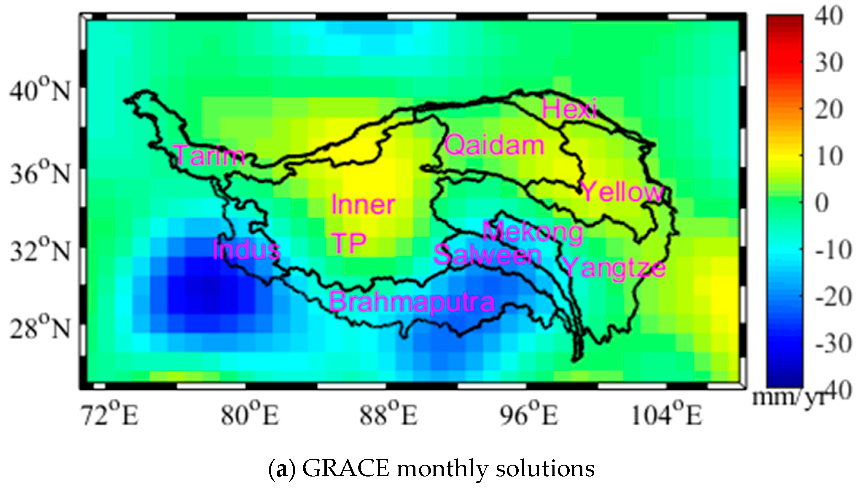
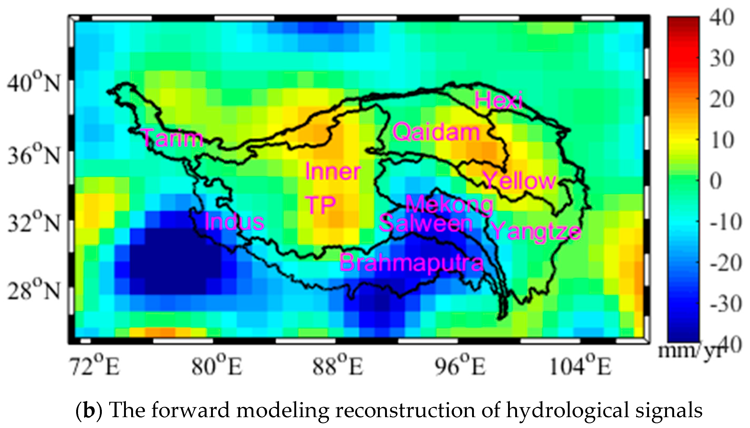
Regional maps of water storage variations on the Tibetan Plateau between August 2002 and December 2016 are shown in Figure 3. From GRACE monthly solutions, we see a significant upward tendency (1.5–2.0 cm/yr) in the total water storage in the central Inner Tibetan Plateau. An increasing tendency is also detected in the Southern Qaidam basin and the Northern Yellow River basin that is characterized by large lakes, such as Qinghai and Har (with surface areas covering 4.5 × 10³ and 1.6 × 10³ km2, respectively). According to our estimates, water storage increased there at a rate of 2.5 cm/yr. This value closely agrees with the results obtained from processing satellite-altimetry data [18,23]. In basins located near the Himalayas and the Hengduan Mountains, on the other hand, we see substantial mass loss. In the Central and Eastern Himalayas, the Brahmaputra, Salween, and Mekong basins attenuating trends are up to −4 cm/yr. This value closely agrees with the results obtained from ICESat and SRTM data, according to which glaciers lost their mass with an elevation change rate of −0.38 m/yr [21]. Both solutions presented in Figure 3 exhibit a secular rate of decreasing water storage (between August 2002 and December 2016). According to a reconstructed trend from hydrological signals, the total water budget over this period decreased at a rate of −6.22 ± 1.24 Gt/yr. A downtrend estimated from the GRACE monthly solutions was at a rate of −2.48 ± 1.69 Gt/yr.
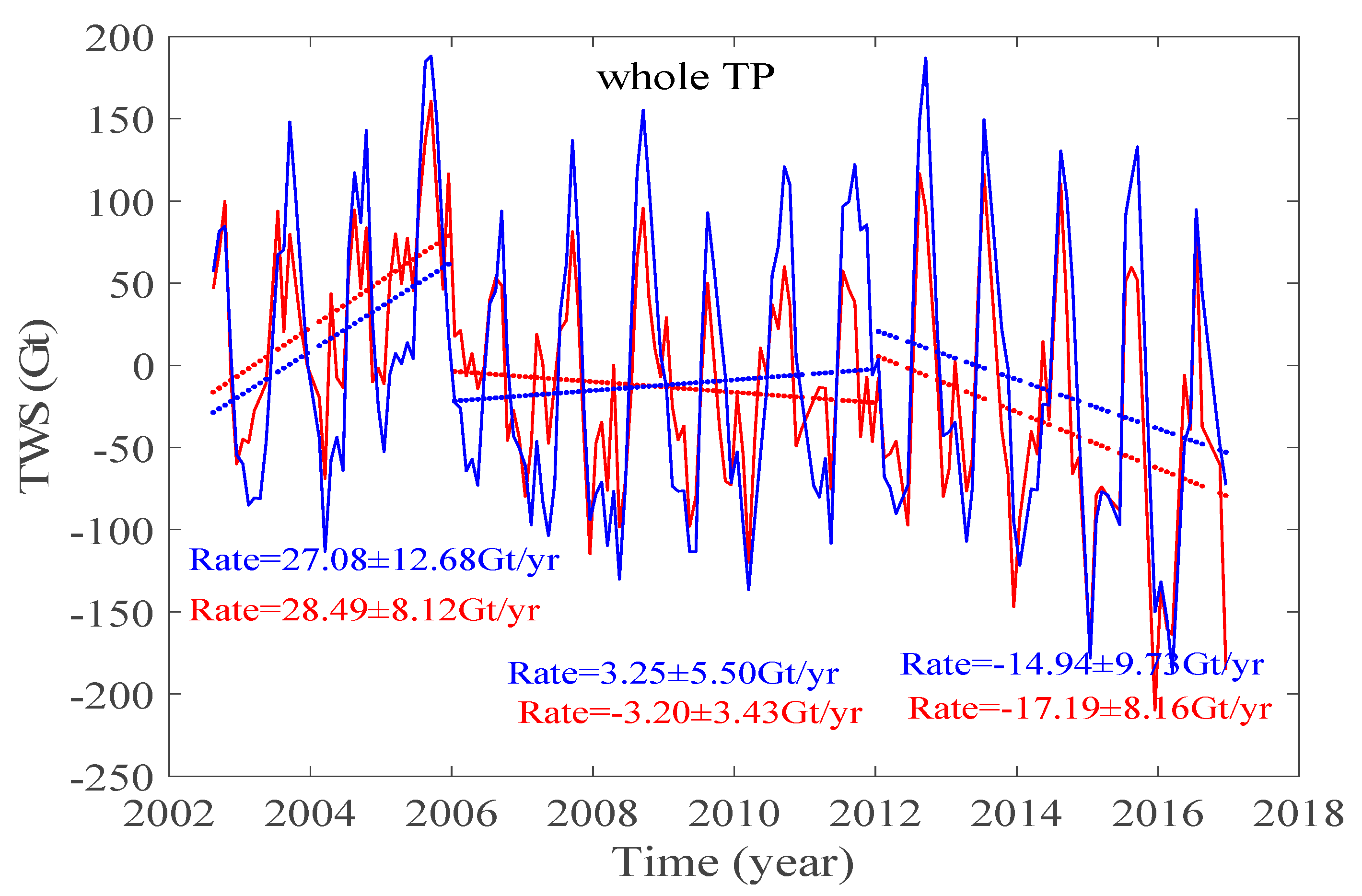
A more detailed inspection of water storage variations indicates a relatively stable trend from the beginning of 2006 to the end of 2011. Much higher rates of inter-annual changes occur before and after this period. To understand better the character of these fluctuations, we divided the whole period into three time intervals, namely from August 2002 to December 2005, from January 2006 to December 2011, and from January 2012 to December 2016. Rates of water storage variations for these three time intervals are shown in Figure 4. From August 2002 to December 2005, the water storage changes are positive at a rate of 27.08 ± 12.68 Gt/yr (from GRACE) and 28.49 ± 8.12 Gt/yr (from a forward modeling). This considerably increasing trend stopped between January 2006 and December 2011. During this period, we see small changes at a rate of 3.25 ± 5.50 Gt/yr (from a forward modeling). For GRACE, we obtained a slightly increasing trend at a rate of −3.2 ± 3.43 Gt/yr. After this relatively stable period, the downtrend again accelerates. According to the result from a forward modeling, the estimated rate from January 2012 to December 2016 reached −17.19 Gt/yr. Similarly, the result from GRACE exhibited a fast decrease at a rate of −14.94 Gt/yr. These findings indicate that the total water storage on the Tibetan Plateau during the investigated period went through a rapid accumulation, followed by a relatively stable and a fast decline variation.
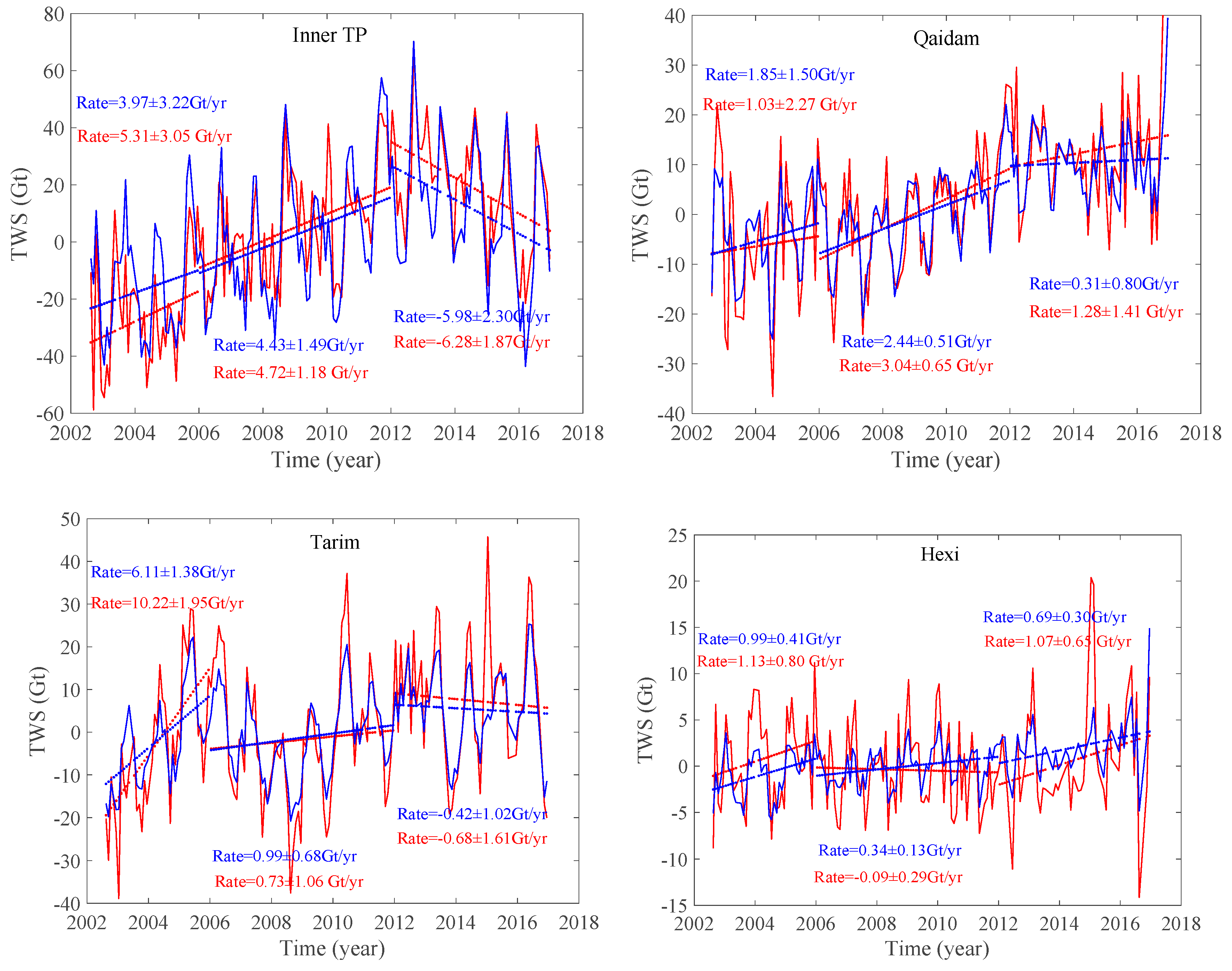
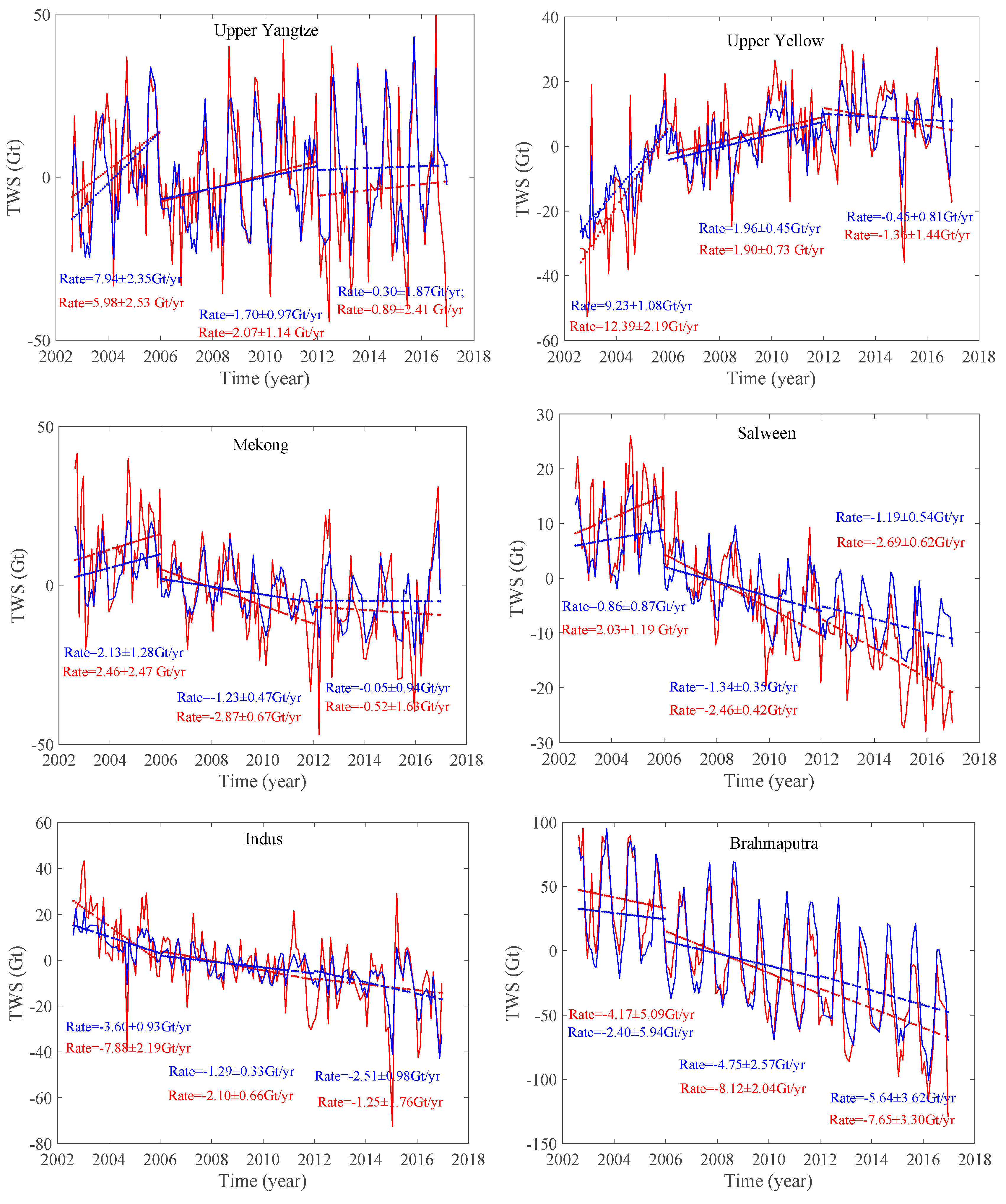
Water storage changes on the Tibetan Plateau exhibit significant spatial heterogeneities (Figure 3) that reflect the unique topography and climatic conditions of its different regions. To illustrate this, we plotted water storage variations individually for each basin (Figure 5). Between August 2002 and December 2005, water storage accumulated in all basins, except the Indus and Brahmaputra basins. From January 2006 to December 2011, water storage continued to decrease in these two basins. Within this period, a decreasing trend also occurred in the Mekong and Salween basins. Total water storage in the Brahmaputra basin showed an astonishing decline at the rate of −8.12 Gt/yr. At the same time, water storage in the Qaidam basin increased at a rate of 3.04 Gt/yr. During the last period, January 2012 to December 2016, we see a quite different pattern. In the Inner Tibetan Plateau, the initial water storage accumulation experiences a declining trend at a rate of −6.28 Gt/yr. The water storage continues increasing only in the Qaidam and Hexi basins. During the entire investigated period over the last 15 years (before 2017), the total water storage increased, except for the Indus, Brahmaputra, Mekong, and Salween basins.
When analyzing the spatial characteristics of water storage variations, the Qaidam and Hexi basins show a mass gain, with increasing inflow of the meltwater from glaciers in the Qilian Mountains. We also see increasing precipitation in these basins. An observed mass loss in the Indus basin was likely induced by the excessive use of groundwater [8,49,50] combined with the effect of increased melting of glaciers in the Western Himalayas [4,22]. A mass gain detected in the Yangtze River and Yellow River basins could be attributed to an increasing melting of Mei Kuang Glacier in the Tangula Mountains and the Dongkemadi Glacier in the Kunlun Mountains due to increasing temperatures [51,52]. Water storage changes in the Inner Tibetan Plateau are likely associated with the combined contribution of precipitation changes and increased river recharge by the inflow of meltwater from glaciers situated in the Kunlun Mountains. Moreover, Xiang et al. [52] and Cheng and Wang [53] detected a large accumulation of groundwater in this basin. According to their findings, the total groundwater volume in the Qiangtang Nature Reserve (located in the central part of the Inner Tibetan Plateau) increased at a rate of 5.37 ± 2.17 Gt/yr.
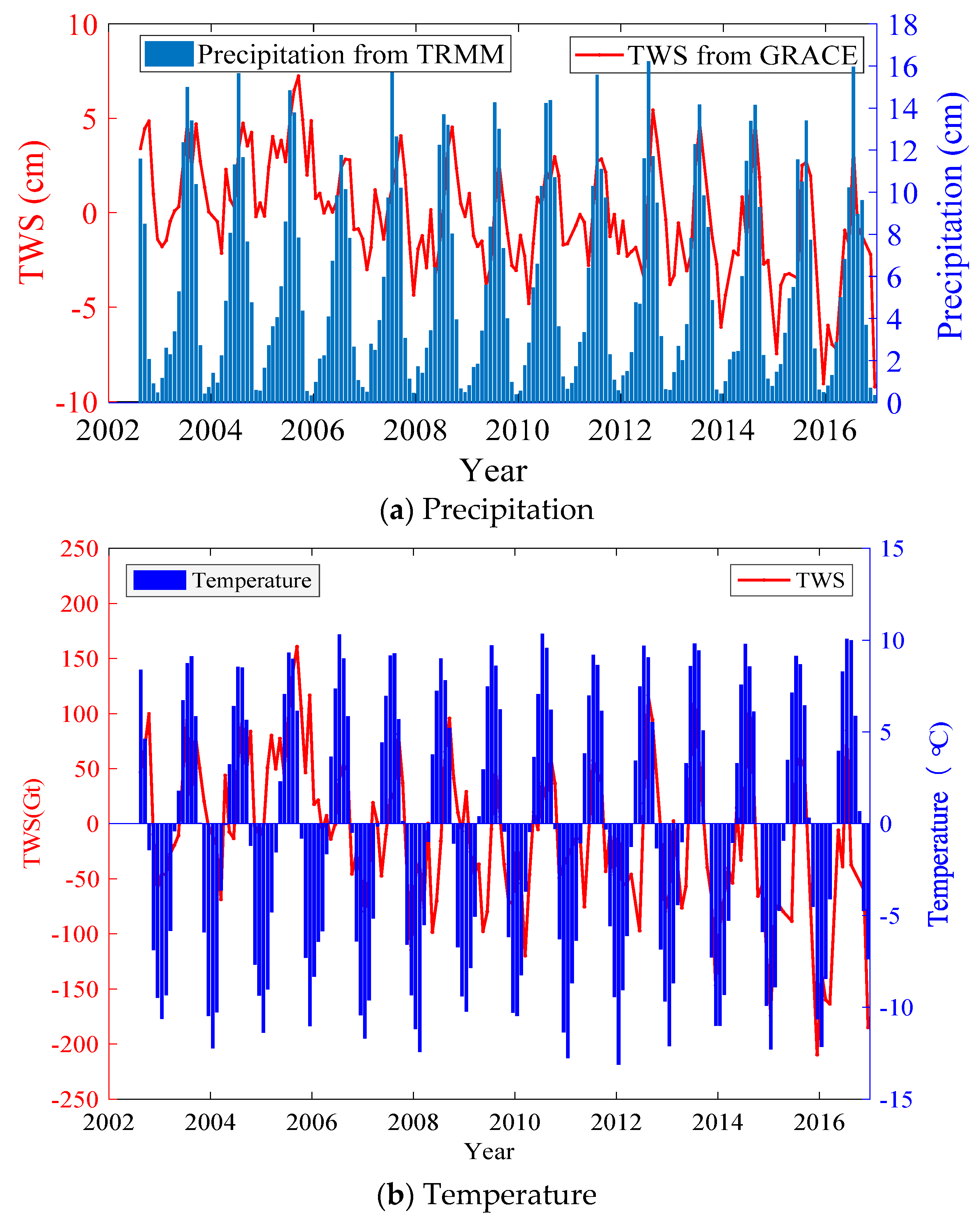
The plateau climate is dominated by a (seasonal) monsoon, which affects precipitation and air temperature in this region. To inspect this factor, we analyzed precipitation extracted from the TRMM-3B43 monthly rainfall data and air temperature from the CNMIC dataset. As seen in Figure 6, the water storage varies with both precipitation and temperature.
When turning our attention to long-term changes in precipitation and air temperature, we recognize that annual rainfall on the Tibet Plateau has not changed considerably over the 15 years prior to 2017 (Table 1). Consequently, precipitation was not a driving factor causing the observed overall decrease in the total water budget on the Tibet Plateau. Instead, increasing temperature could be a principal reason, causing glacial and snowmelt, thus indirectly affecting the water regime of lakes. The average air temperature on the entire plateau increased at the annual rate of 0.03 °C over the investigated period, which supports this assumption.
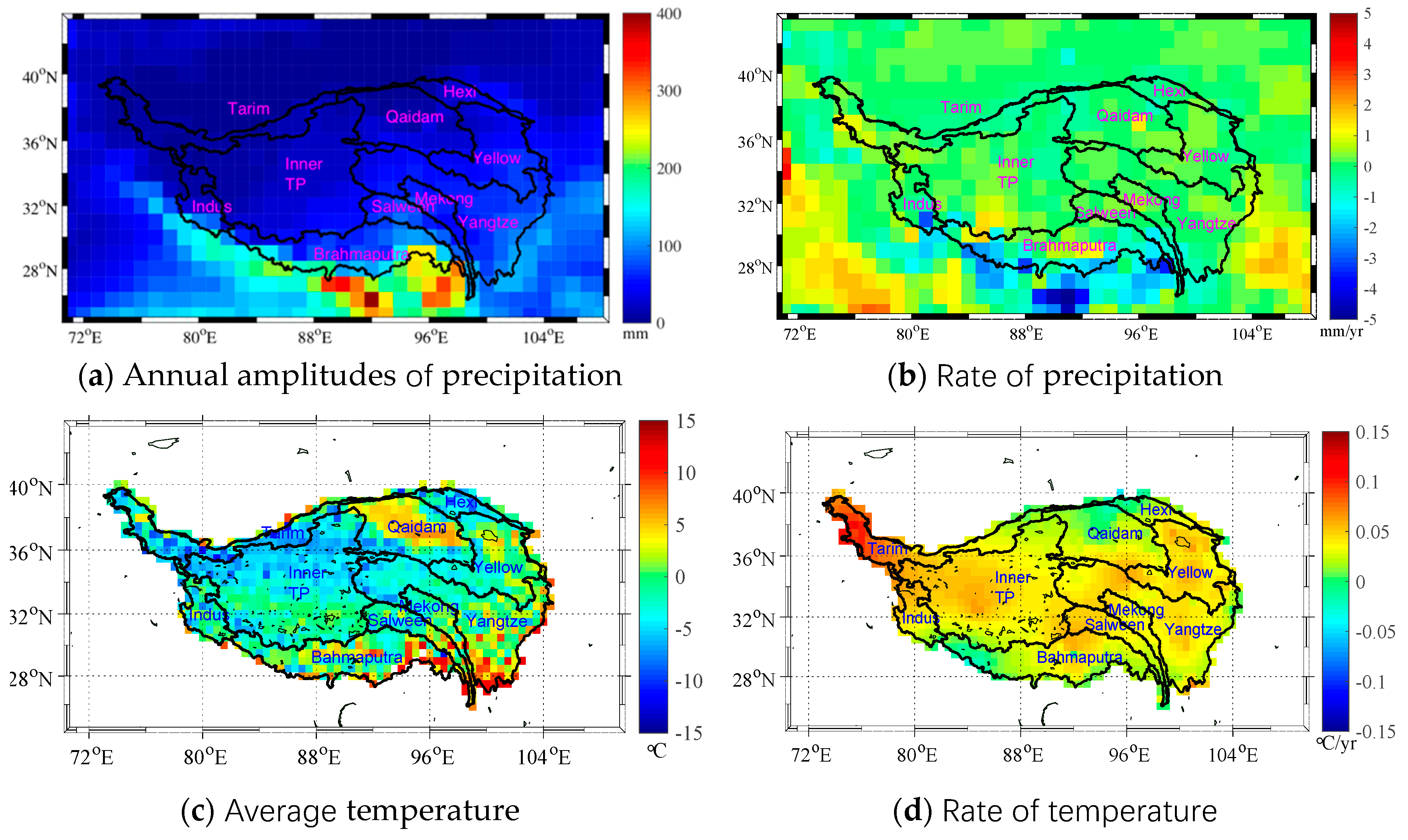
To analyze factors that likely influenced water storage variations in particular basins, we analyzed precipitation and air temperature in Figure 7. The annual precipitation rate over most of the Tibetan Plateau exhibited more or less a stable pattern, except for a decreasing trend in the Himalayas and the Hengduan Mountains (Figure 7b). Air temperature increased over most of the plateau (Figure 7c). Maxima up to about 0.15 °C/yr are detected in the Tarim and Indus basins. A decreasing temperature at a rate to about −0.1 °C/yr is detected in parts of the Central Himalayas and in the Qaidam and Hexi basins.
Recent studies of elevation and ice mass changes of glaciers revealed their rapid decrease [16,21,22]. This decline was especially dramatic in the Himalayas and the Hengduan Mountains, with a rapid decrease of glacier volumes or their complete disappearance. This trend is confirmed by our results in Figure 3b, showing that the total water budget in those regions significantly declined. This trend could possibly be explained by glacier melting and run-off of the meltwater into several major exorheic rivers in these regions. The rate of glacial melting in the Hengduan Mountain reached −20 mm/yr and between −10 and −20 mm/yr in the Himalayas. Overall, glaciers in the Western and Eastern Himalayas exhibited faster rates of melting than glaciers in the central part. This finding agrees with the ICESat results [18]. Substantial glacial retreat was also confirmed in the Tanggula Mountains. On the other hand, we observe a positive trend at locations of glaciers in the Kunlun and Qilian Mountains. This unexpected tendency needs further analysis due to the unique local climate of those parts of Tibet.
4.1.2. Signal Leakage
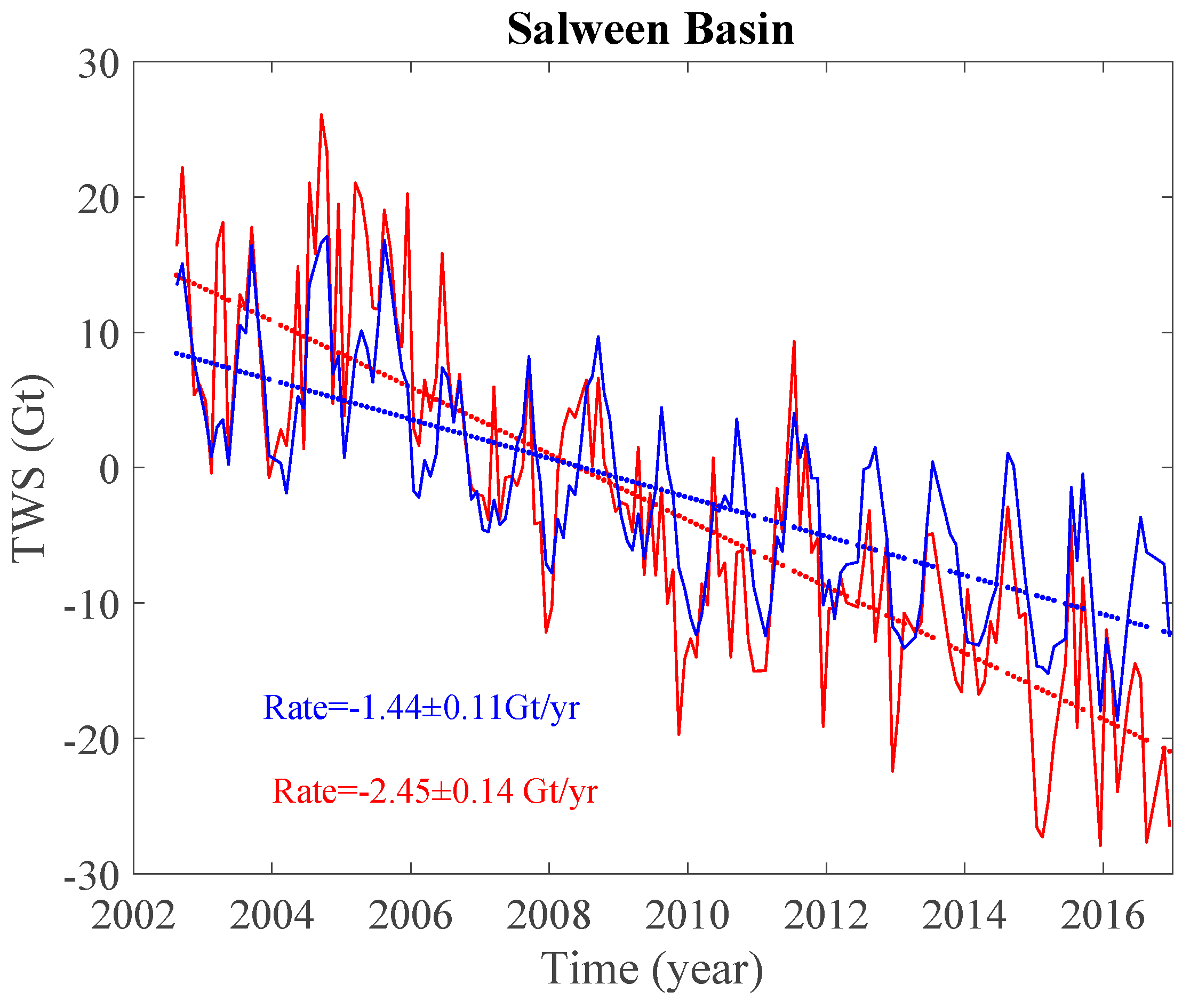
As stated above, our estimates of water storage variations (shown in Figure 5) are influenced by a signal leakage. Apparently, the most concerning of our estimates is in the Indus and Brahmaputra basins. The former is affected mainly by ground water depletion in Northwest India, and the latter is influenced by decreasing precipitation in the Eastern Himalayas. To better understand how much these hydrological signals affect our estimates, we applied a forward modeling technique to estimate water storage variations in two neighboring regions with high negative trends from August 2002 to December 2016 (Region 1: 28°–32° N, 74°–78° E of Northwest India, and Region 2: 88°–92° E, 25°–28° N of the Eastern Himalayas) (Figure 8). For comparison, we also plotted water storage variations in the Indus and Brahmaputra basins over the same period. As seen in Figure 8a, the water budget in Region 1 decreased at a rate of −13.15 Gt/yr. Over the same period, the water budget in the Indus basin decreased at a rate of −3.58 Gt/yr. This value agrees quite well with the result presented by Brun et al. [54]. According to their estimates from ICESat and ASTER, glacier loss in the Indus basin occurred at a rate of about −4 Gt/yr. The water budget in Region 2 (Figure 8b) shows a decreasing precipitation at a rate of −6.19 Gt/yr. The water budget in the Brahmaputra basin decreased at a rate of −8.47 Gt/yr. In both cases, we recognize some similarities in temporal variations of water storage between basins and their neighboring regions. Moreover, hydrological signals in the Brahmaputra basin and Region 2 are characterized by large and relatively regular seasonal variations. In contrast, a seasonal monsoon pattern in the Salween basin is not clearly manifested (Figure 9).
4.1.3. Seasonal Changes
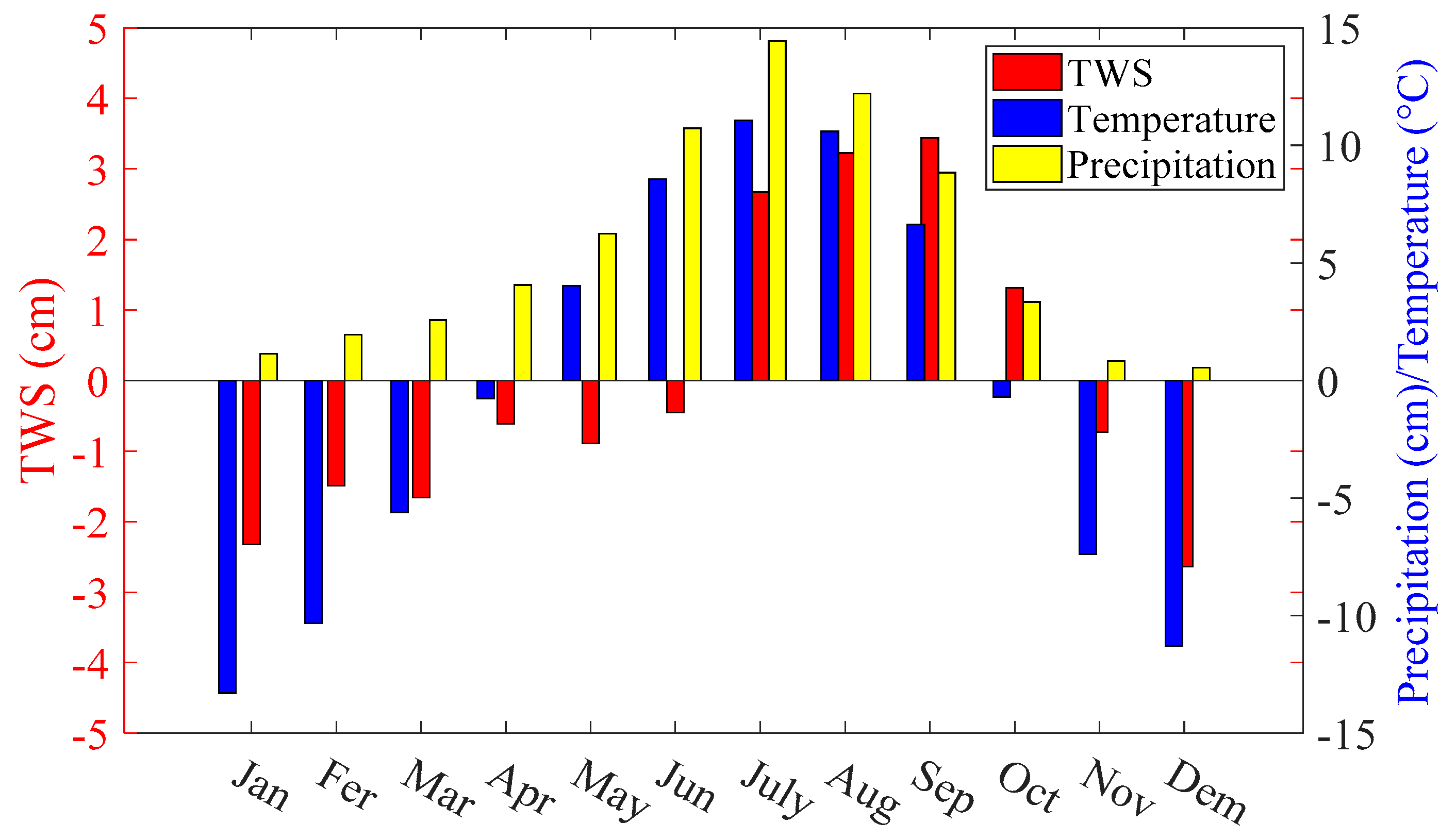
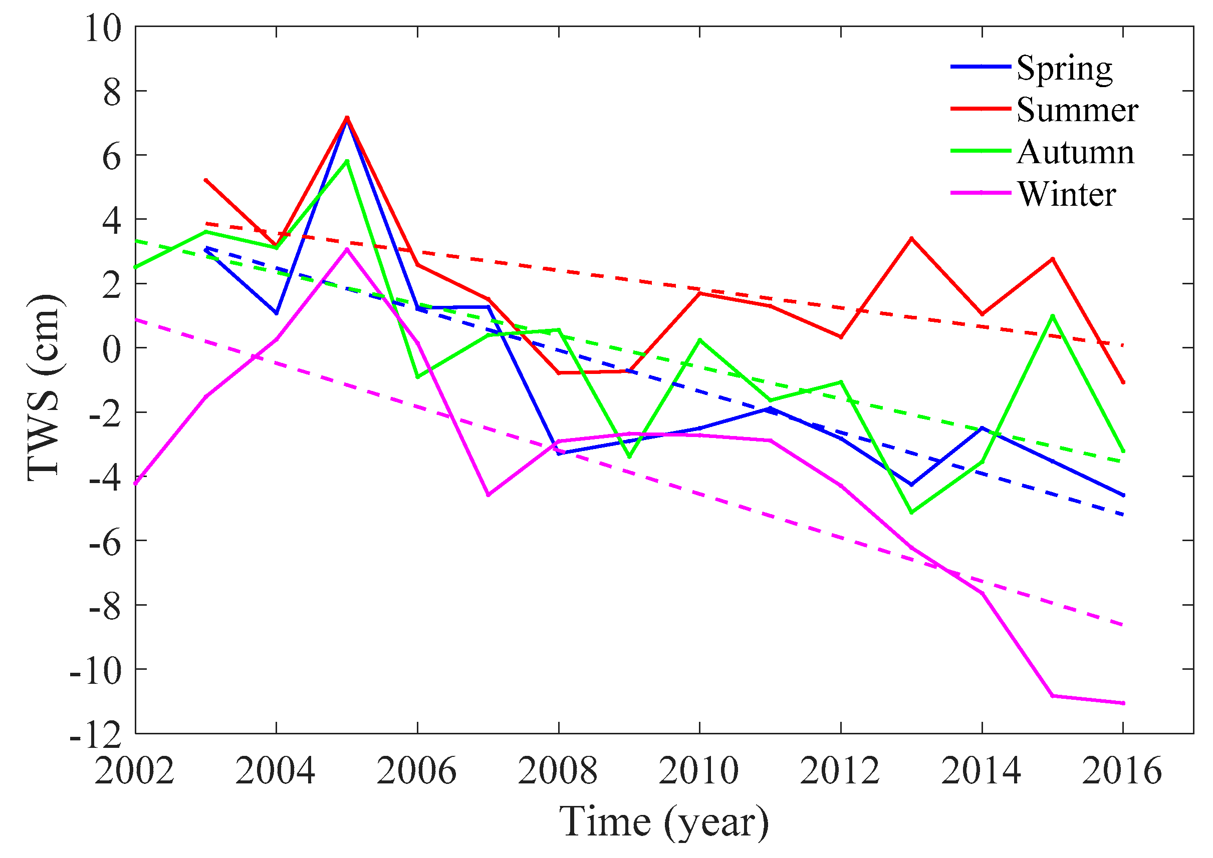
Monthly means of water storage, temperature, and precipitation averaged over the period investigated are shown in Figure 10. In addition, seasonal trends of water storage variations for the same period during spring, summer, autumn, and winter are plotted in Figure 11. The water budget of the Tibetan Plateau exhibits relatively large annual oscillations (Figure 10). In summer, tropospheric tropical easterlies, subtropical westerlies, stratospheric easterlies, and the southwestern monsoon from the Indian Ocean [15] bring a significant amount of rain, causing maximum precipitation between June and September [9]. A large amount of rainwater that accumulates on the Tibetan Plateau during wet summer months causes an overall increase in the total water budget, reaching maxima typically in September. Dry and cold winter periods are characterized by an overall water mass loss mainly due to river water run-off, reflecting very low precipitation. Nonetheless, regardless of season, water storage generally decreased (Figure 11). After reaching maxima in 2005, the fastest decrease in the total water budget of the plateau occurred during each winter, confirming temperature increase as a dominant factor.
4.2. Water Level and Glacier Changes from ICESat
The results presented in Section 4.1 reveal a relatively complex temporal pattern of water mass balance on the Tibetan Plateau, with a relatively stable period overall water budget and periods of rapid changes. Since annual precipitation rates did not change significantly, this pattern could be explained by changes in the water budgets of glaciers and lakes. This is particularly relevant to an increasing water budget of mountain lakes due to ongoing glacial and snow melting that might temporarily occur over a certain period and eventually modify the overall trend. According to existing studies, water mass variations are attributed either to glacial melting [22] or to the water balance of lakes [23]. To inspect these two phenomena, we applied a localized analysis of the ICESat data (from March 2003 to October 2009) for selected major lakes and glaciers.
4.2.1. Water Level Changes of Major Lakes
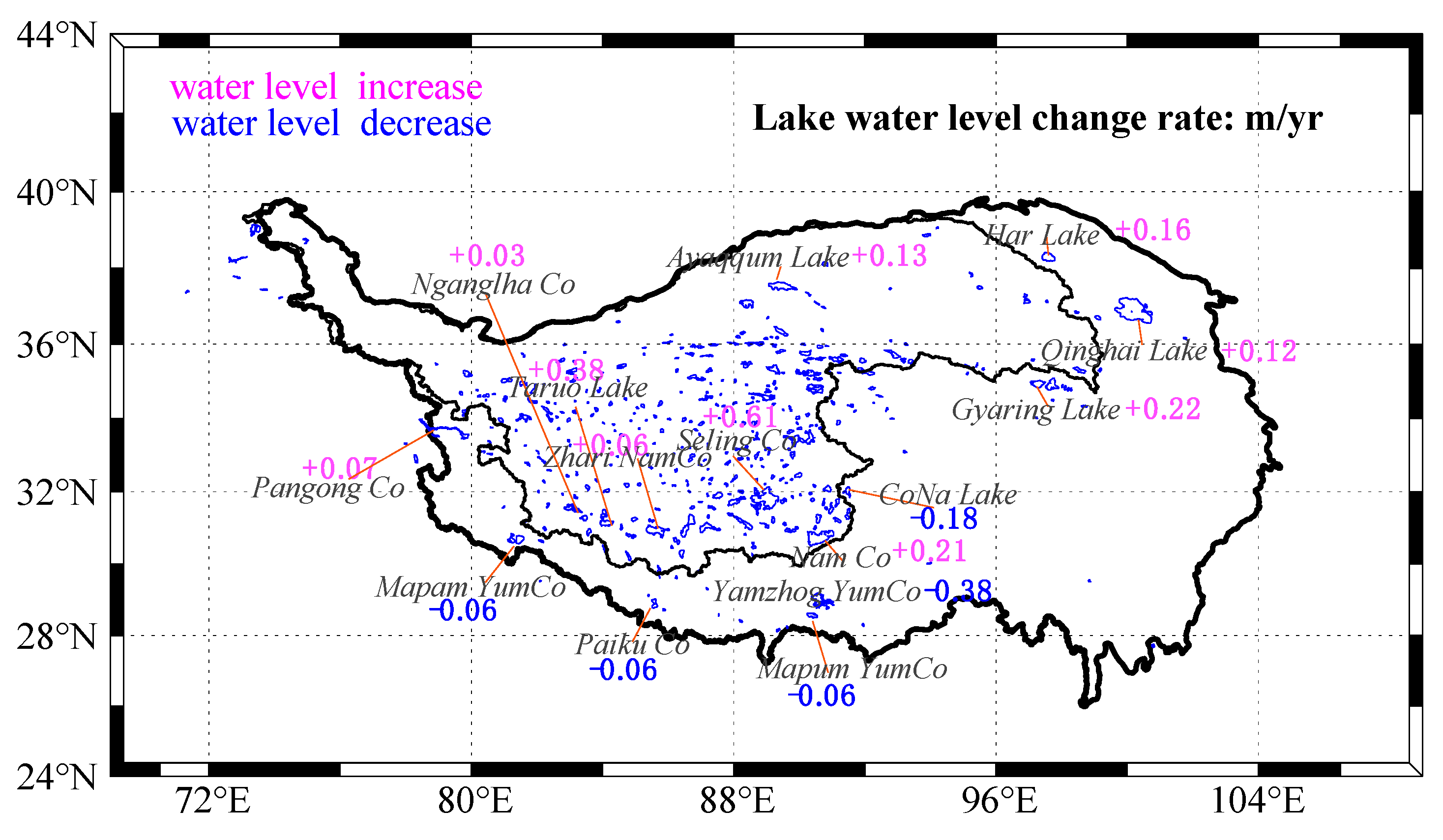
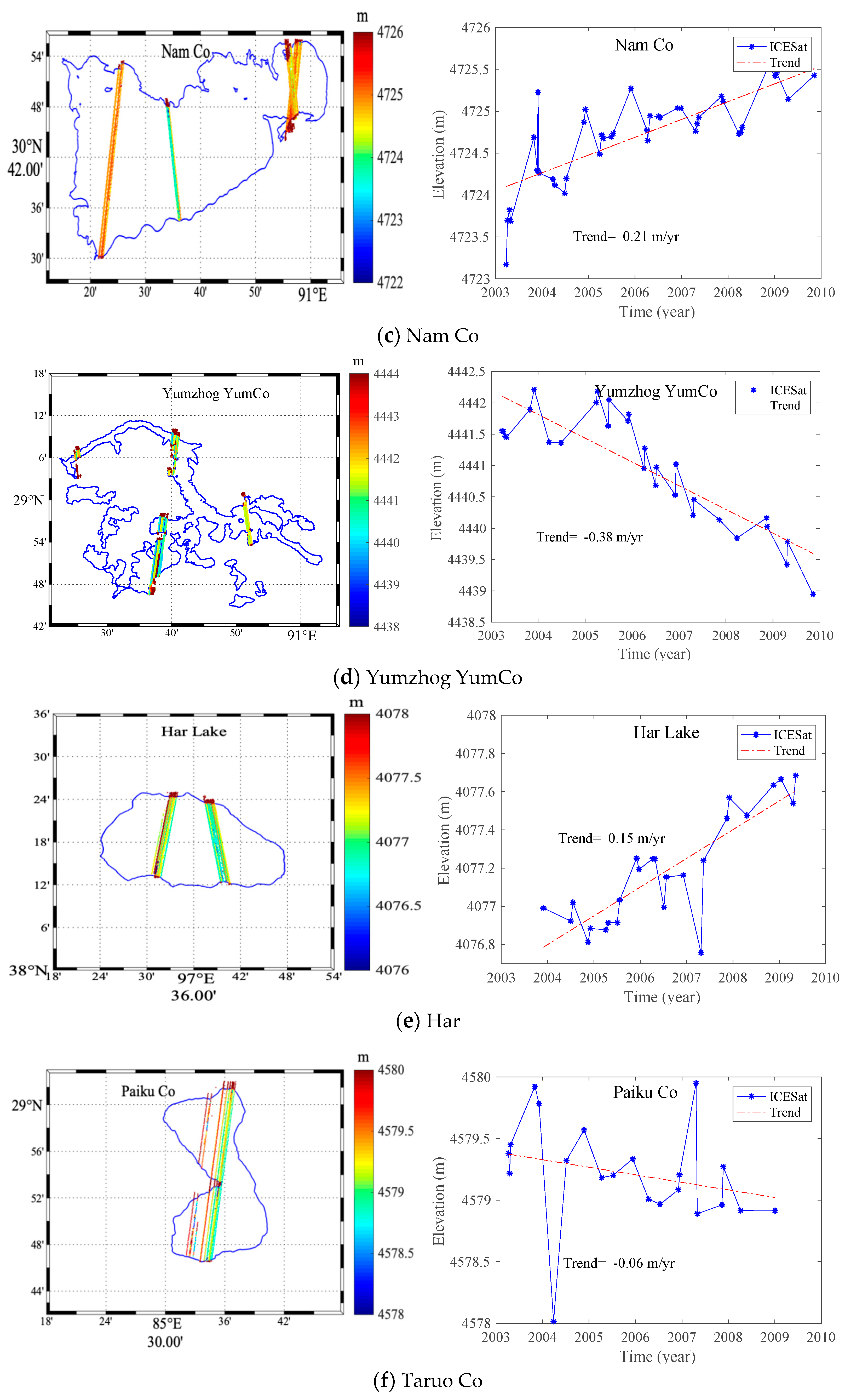
There are more than 1500 lakes in Tibet that are mainly distributed in the Himalayas, the Kunlun Mountains, and the Qaidam basin, with a maximum concentration on the Changtang Plateau (Figure 1). We selected 15 major lakes to estimate water level changes by processing ICESat data. Estimated trends of water level changes are shown in Figure 12. We also plotted their annual rates in Figure 13. As seen, Yumzhog Yumco (located in vicinity of the Himalayas) is characterized by a decreasing trend at a rate of −0.38 m/yr. Similarly, Mapam YumCo shows a decreasing trend at a rate of −0.06 m/yr. Qinghai, Nam Co, Seling Co, and Har have increasing trends, with a maximum water level increase of 0.62 m/yr in Seling Co.
Geographic information of 15 selected major lakes on the Tibetan Plateau and their water level changes from the ICESat data (between March 2003 and October 2009) are summarized in Table 2. In the Northeast Tibetan Plateau, the ICESat results confirmed increasing trends of water budgets of Har, Qinghai, and Gyaring. Har and Qinghai are salt lakes. Moreover, Qinghai is the largest salt lake (roughly 4317.69 km2 in 2014) in China. Ground in situ measurements revealed a declining trend in this lake water level at a rate of −0.081 m/yr between 1959 and 2000 [55]. However, our estimate from ICESat over the period 2003–2009 indicates that the water level increased at a rate of 0.11 m/yr. This value actually agrees closely with the in situ measurements taken over the same period (0.11 m/yr [56]). Har receives a water recharge of glacier melt from the Qilian Mountains. The ICESat result shows an increasing trend in this lake’s water level at a rate of 0.15 m/yr. In the Central Tibetan Plateau, the ICESat results show an increasing trend for most lakes. Meltwater was a considerable contributor for lakes that are near glaciers, such as Seling Co and Taruo Co in the Southeast Inner Tibetan Plateau. In contrast, the ICESat results indicate decreasing trends of Yamzhog YumCo, Paiku Co, and Mapam YumCo located in the Southern Tibetan Plateau in proximity of the Himalayas. An accelerating decrease of Yamzho YumCo was mainly due to human activity since 2005. As a hydrologically closed alpine lake, changes in the lake level of Paiku Co and Puma YumCo are mainly associated with glacier/snow run-off, precipitation on the surface of lakes, precipitation-induced run-off, and lake evaporation [57]. Over the last 40years, glaciers in the Himalayas retreated and thinned rapidly [8]. Since glacial lakes and glaciers are connected, the glacial lake expansion largely depends on glacial retreat. A lake shrinkage near the Himalayas may be only part of a large-scale climate drought due to a decrease in the monsoon precipitation [58] (see also Figure 7b).
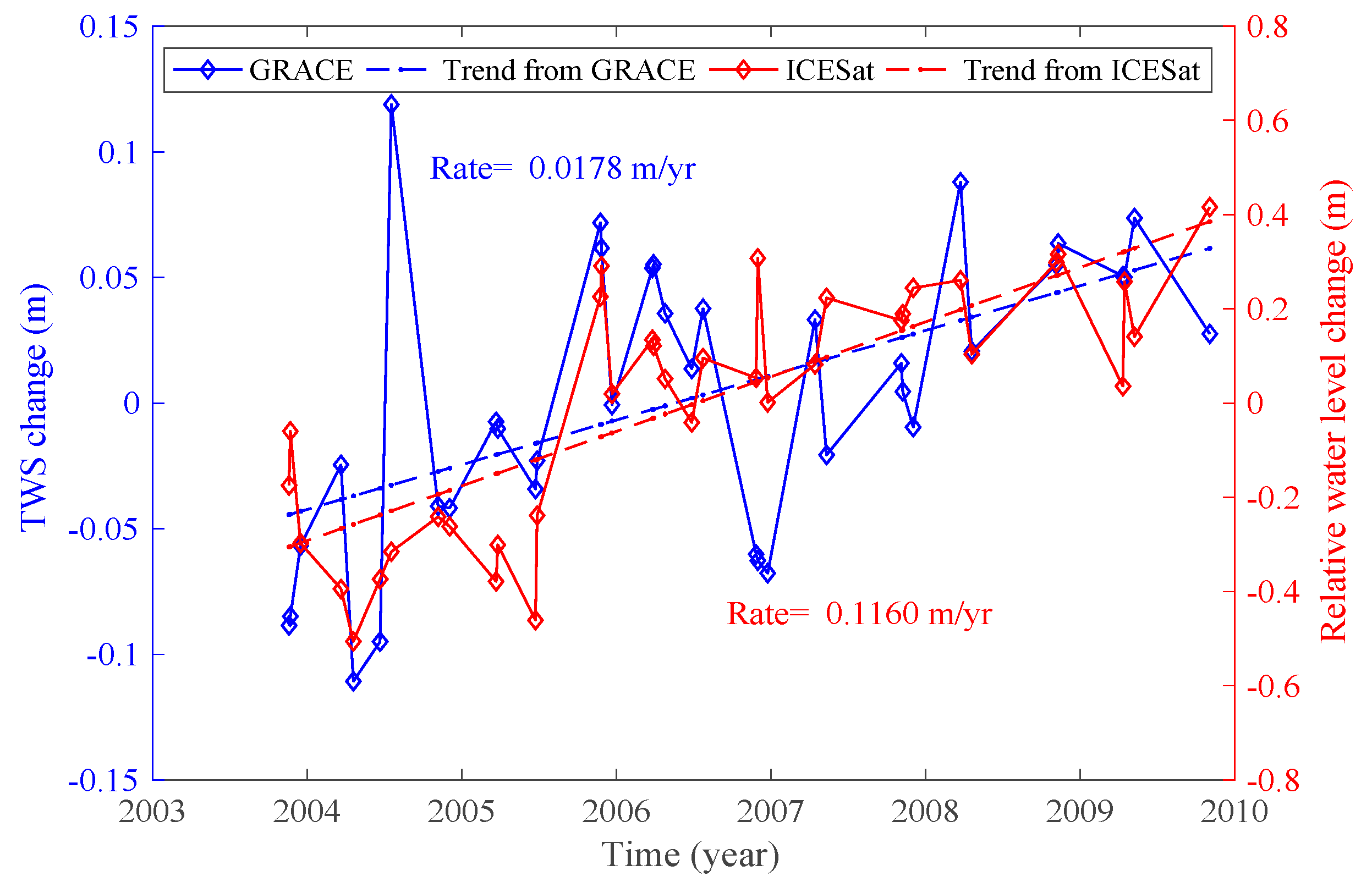
Some studies indicate possibilities of using the GRACE data to monitor water storage variations of relatively small lakes, such as Qinghai [59,60]. This is possible especially if their hydrological signal is quite isolated from other signals. To illustrate this, we plotted time series of the annual rates of the ICESat water level change and the GRACE water storage change for Qinghai Lake in Figure 14. Though both results exhibit overall similarities in their secular trends, significant annual (as well as inter-annual) inconsistencies are obvious.
4.2.2. Elevation Changes of Major Glaciers
A recent analysis of elevation changes of glaciers revealed their rapid shrinking in the Himalayas and the Hengduan Mountains. Glaciers in the Karakoram and West Kunlun Mountains are, on the other hand, relatively stable [16,21,22]. Water mass variations estimated from GRACE in the Himalayas and the Hengduan Mountains are significantly negative. The glacial melting rate in the Hengduan Mountain reached −20 mm/yr and in the Himalayas between −10 and −20 mm/yr. Overall, glaciers in the Western and Eastern Himalayas exhibited faster rates of melting than glaciers in the central part. This finding agrees with results from the ICESat data analysis [18]. A substantial glacial retreat was also confirmed in the Tanggula Mountains. On the other hand, we recognize a positive trend at the locations of glaciers in the Kunlun and Qilian Mountains.
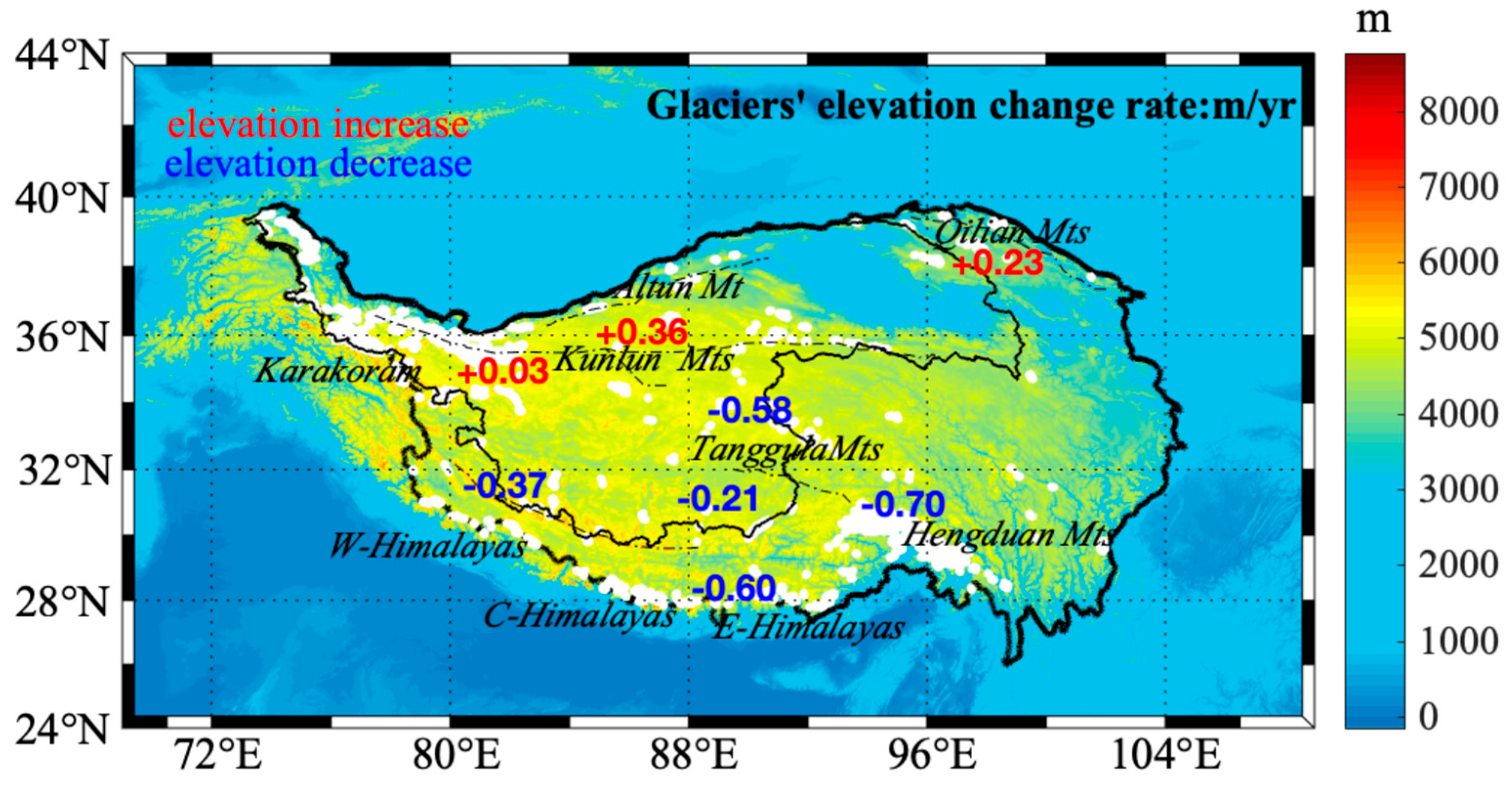
We used ICESat data to investigate elevation changes of large glaciers on the Tibetan Plateau. The results are presented in Figure 15. Glaciers of the Qilian and Altun Mountains (in the northern part of the plateau) and glaciers of the Kunlun Mountains (in the central part) show increasing trends. In the Himalayas and the Hengduan Mountains, the ICESat (as well as GRACE) results indicate a rapid decrease of glacier volumes and elevations. For glaciers located in the Hengduan Mountains, for instance, glacier elevations decreased at a rate of about −0.7 m/yr and the glacier mass loss was at a rate of −0.02 m/yr.
5. Summary and Discussion
We have investigated water storage variations on the Tibetan Plateau using the GRACE monthly solutions. To suppress overall leakage between land and ocean, we applied the forward modeling restoration of hydrological signals. In addition, we considered the secular GIA trend. We also investigated elevation changes in large lakes and glaciers from the ICESat data to identify the most significant contributions to changes in water storage on the Tibetan Plateau. According to our results, the total water budget on the Tibetan Plateau decreased at an average rate of −6.22 ± 1.74 Gt/yr between August 2002 and December 2016. During this 15-year period however, inter-annual variations were rather uneven. The detected mass gain at a rate of 28.49 ± 10.40 Gt/yr (between August 2002 and December 2005) was followed by a relatively stable period (between January 2006 and December 2011) and a fast decline at a rate of −17.19 Gt/yr (between January 2012 and December 2016). The ICESat data analysis of selected major lakes and glaciers confirmed a relatively close spatial coherence, with a prevailing glacial melting in the Himalayas and a typically increasing water budget of lakes on the Tibetan Plateau.
Significant inconsistencies exist in estimated values of the total water budget on the Tibetan Plateau. The total mass gain in Tibet and the Qilian Mountains over the period 2003–2010 at a rate of 7 Gt/yr was, for instance, reported by Jacob et al. [22]. They analyzed the GRACE gravity data and concluded that over this period the total mass volume of glaciers increased. An increasing trend during 2003–2012 was also reported by Kaab et al. [21], and Jin and Zou [40]. Song et al. [23] gave a different explanation. They suggested that this positive trend was mainly due to water accumulations in lakes on the Tibetan Plateau (see also Zhang et al. [3]). Compared to these studies, other estimates based on a combined processing of GRACE and ICESat data [18,20,28] indicated a significant mass loss over similar periods, explained by glacial melting on the Tibetan Plateau. The results presented in this study confirm that the total water budget in Tibet over the last 15 years (before 2017) decreased substantially, except for a relatively stable period between August 2002 and December 2007. A possible explanation of this stable period might be given by a rebalance of total mass loss (due to the glacier melting in Tibet) by a temporal filling of lakes by the melted ice and show. This is supported by our observed stable precipitation but an increasing temperature over the investigated period.
According to our findings, an overall decrease in the total water budget on the Tibetan Plateau likely reflects mainly glacial melting due to increasing temperature on the plateau. Seasonal variations were driven mostly by annual changes in precipitation, with maxima in summer and minima in the dry and cold winter seasons of the plateau.
Since we applied the forward modeling to suppress overall leakage of GRACE solutions in Tibet, this method still depends on the assumptions adopted in numerical simulations, which could be affected by large uncertainties [61]. A major reason is a lack of in situ observations that could be used to verify the effectiveness and to assess the accuracy of this method. Moreover, this method cannot mitigate signal leakage among different basins on land. This is evident from our estimates of water storage variations in the Western Himalayas that are affected by significant leakage in the signal from groundwater depletion in Northwest India. Some lakes in the Inner Tibetan Plateau basin located near the Indus basin show a negative trend, while the actual water level of these lakes has been rising. The water level of Tarong Co (81.8° N, 29.4° E), for instance, increased by 2.04 m [18]. Furthermore, additional errors are attributed to parameters used for computing leakage reduction.
Previous studies have demonstrated that water level changes in lakes determined from ICESat/GLAS altimetry agree relatively closely with those determined from in situ gauge observations [55,56]. However, some intra-annual fluctuations in water level could not be detected due to limitations of ICESat. Therefore, a bias in water level trends may be inevitable for limited campaigns. The complex terrain geometry also worsens the accuracy. This particularly applies for glaciers situated in the Himalayas and the Western Tibet Plateau, where large elevation gradients significantly affect estimates of glacier elevation changes from relatively sparse tracks of ICESat.
The Tibetan Plateau is located in central Asia with the highest mountain and extraordinary size, The Glacial Isostatic Adjustment (GIA) effect has large uncertainty in the Tibetan Plateau because the past and present dimensions of ice sheets are suffering from large uncertainties. Larger differences in GIA estimates are found from different models or analyses based on the possible ice sheet and glacial history in Tibet [62], which may affect estimation of water storage variations from GRACE solutions in Tibet.
Author Contributions
Z.F. performed numerical studies and prepared a draft of manuscript; T.R. and J.S.G. coordinated this research and compiled the final version of the manuscript.
Funding
This research was funded by the Hong Kong Research Grants Council, Project 1-ZE8F: Remote-sensing data for studying Earth’s and planetary inner structure, Strategic Priority Research Program Project of the Chinese Academy of Sciences under contact #XDA23040100, Jiangsu Province Distinguished Professor Project under contact #R2018T20 and Startup Foundation for Introducing Talent of NUIST.
Conflicts of Interest
The authors declare no conflict of interest. The founding sponsors had no role in the design of the study; in the collection, analyses, or interpretation of data; in the writing of the manuscript; or in the decision to publish the results.
References
- Tapponnier, P.; Zhiqin, X.; Roger, F.; Meyer, B.; Arnaud, N.; Wittlinger, G.; Jingsui, Y. Oblique stepwise rise and growth of the Tibet Plateau. Science 2001, 294, 1671–1677. [Google Scholar] [CrossRef]
- Dewey, J.F.; Shackleton, R.M.; Chengfa, C.; Yiyin, S. The tectonic evolution of the Tibetan Plateau. Philos. Trans. R. Soc. Lond. A 1988, 327, 379–413. [Google Scholar] [CrossRef]
- Zhang, G.; Yao, T.; Xie, H.; Kang, S.; Lei, Y. Increased mass over the Tibetan Plateau: From lakes or glaciers? Geophys. Res. Lett. 2013, 40, 2125–2130. [Google Scholar] [CrossRef] [Green Version]
- Rodell, M.; Velicogna, I.; Famiglietti, J.S. Satellite-based estimates of groundwater depletion in India. Nature 2009, 460, 999. [Google Scholar] [CrossRef] [PubMed]
- Rodell, M.; Famiglietti, J.S. Detectability of variations in continental water storage from satellite observations of the time dependent gravity field. Water Resour. Res. 1999, 35, 2705–2723. [Google Scholar] [CrossRef] [Green Version]
- Guo, N.; Jie, Z.; Yun, L. Climate change indicated by the recent change of inland lakes in Northwest China. J. Glaciol. Geocryol. 2003, 2, 16. [Google Scholar]
- Cheng, G.; Wu, T. Responses of permafrost to climate change and their environmental significance, Qinghai-Tibet Plateau. J. Geophys. Res. Earth Surf. 2007, 112, F2. [Google Scholar] [CrossRef]
- Yao, T.; Thompson, L.; Yang, W.; Yu, W.; Gao, Y.; Guo, X.; Yang, X.; Duan, K.; Zhao, H.; Xu, B.; et al. Different glacier status with atmospheric circulations in Tibetan Plateau and surroundings. Nat. Clim. Chang. 2012, 2, 663. [Google Scholar] [CrossRef]
- Liu, X.; Chen, B. Climatic warming in the Tibetan Plateau during recent decades. Int. J. Clim. 2000, 20, 1729–1742. [Google Scholar] [CrossRef] [Green Version]
- Liu, J.; Wang, S.; Yu, S.; Yang, D.; Zhang, L. Climate warming and growth of high-elevation inland lakes on the Tibetan Plateau. Glob. Planet. Chang. 2009, 67, 209–217. [Google Scholar] [CrossRef]
- Ye, Q.H.; Yao, T.D.; Naruse, R.J. Glacier and lake variations in the Mapam Yumco basin, Western Himalayas, Tibetan Plateau, from 1974 to 2003 using remote sensing and GIS technologies. J. Glaciol. 2008, 54, 933–935. [Google Scholar] [CrossRef]
- Xiangde, X.; Shiyan, T.; Jizhi, W.; Lianshou, C.; Li, Z.; Xiurong, W. The relationship between water vapor transport features of Tibetan Plateau-monsoon “large triangle” affecting region and drought-flood abnormality of China. Acta Meteorol. Sin. 2002, 60, 257–266. [Google Scholar]
- Gardelle, J.; Berthier, E.; Arnaud, Y.; Kääb, A. Region-wide glacier mass balances over the Pamir–Karakoram-Himalaya during 1999–2011. Cryosphere 2013, 7, 1263–1286. [Google Scholar] [CrossRef]
- Li, Z.; Sun, W.; Zeng, Q. Measurements of glacier variation in the Tibetan Plateau using Landsat data. Remote Sens. Environ. 1998, 63, 258–264. [Google Scholar] [CrossRef]
- Junfeng, W.; Shiyin, L.; Wanqin, G.; Xiaojun, Y.; Junli, X.; Weijia, B.; Zongli, J. Surface-area changes of glaciers in the Tibetan Plateau interior area since the 1970s using recent Landsat images and historical maps. Ann. Glaciol. 2014, 55, 213–222. [Google Scholar] [CrossRef] [Green Version]
- Gardner, A.S.; Moholdt, G.; Cogley, J.G.; Wouters, B.; Arendt, A.A.; Wahr, J.; Ligtenberg, S.R. A reconciled estimate of glacier contributions to sea level rise: 2003 to 2009. Science 2013, 340, 852–857. [Google Scholar] [CrossRef]
- Qinghua, Y.E.; Zong, J.; Tian, L.; Graham, C.J.; Song, C.; Guo, W. Glacier changes on the Tibetan plateau derived from landsat imagery: mid-1970s—2000–13. J. Glaciol. 2017, 63, 273–287. [Google Scholar]
- Song, C.; Bo, H.; Linghong, K. Modeling and analysis of lake water storage changes on the Tibetan Plateau using multi-mission satellite data. Remote Sens. Environ. 2013, 135, 25–35. [Google Scholar] [CrossRef]
- Liu, W.; Guo, Q.H.; Wang, Y.X. Temporal-spatial climate change in the last 35 years in Tibet and its geo-environmental consequences. Environ. Geol. 2008, 54, 1747–1754. [Google Scholar] [CrossRef]
- Zhang, G.; Xie, H.; Kang, S.; Yi, D.; Ackley, S.F. Monitoring lake level changes on the Tibetan Plateau using ICESat altimetry data (2003–2009). Rem. Sens. Environ. 2011, 115, 1733–1742. [Google Scholar] [CrossRef]
- Kääb, A.; Berthier, E.; Nuth, C.; Nuth, C.; Gardelle, J.; Arnaud, Y. Contrasting patterns of early twenty-first-century glacier mass change in the Himalayas. Nature 2012, 488, 495. [Google Scholar] [CrossRef]
- Jacob, T.; Wahr, J.; Pfeffer, W.T.; Swenson, S. Recent contributions of glaciers and ice caps to sea level rise. Nature 2012, 482, 514. [Google Scholar] [CrossRef]
- Song, C.; Ke, L.; Huang, B.; Richards, K.S. Can mountain glacier melting explains the GRACE-observed mass loss in the southeast Tibetan Plateau: From a climate perspective? Glob. Planet. Chang. 2015, 124, 1–9. [Google Scholar] [CrossRef]
- Matsuo, K.; Heki, K. Time-variable ice loss in Asian high mountains from satellite gravimetry. Earth Planet. Sci. Lett. 2010, 290, 30–36. [Google Scholar] [CrossRef] [Green Version]
- Zwally, H.J.; Schutz, B.; Abdalati, W.; Abshire, J.; Bentley, C.; Brenner, A.; Herring, T. ICESat’s laser measurements of polar ice, atmosphere, ocean, and land. J. Geodynam. 2002, 34, 405–445. [Google Scholar] [CrossRef]
- Wan, W.; Long, D.; Hong, Y.; Ma, Y.; Yuan, Y.; Xiao, P.; Gu, X. A lake data set for the Tibetan Plateau from the 1960s, 2005, and 2014. Sci. Data 2016, 3, 160039. [Google Scholar] [CrossRef]
- Guo, W.; Liu, S.; Xu, J.; Wu, L.; Shangguan, D.; Yao, X.; Jiang, Z. The second Chinese glacier inventory: Data, methods and results. J. Glaciol. 2015, 61, 357–372. [Google Scholar] [CrossRef]
- Wang, Q.; Yi, S.; Sun, W. The changing pattern of lake and its contribution to increased mass in the Tibetan Plateau derived from GRACE and ICESat data. Geophys. J. Int. 2016, 207, 528–541. [Google Scholar] [CrossRef]
- Yi, S.; Sun, W. Evaluation of glacier changes in high-mountain Asia based on 10 year GRACE RL05 models. J. Geophys. Res. Solid Earth 2014, 119, 2504–2517. [Google Scholar] [CrossRef] [Green Version]
- Neckel, N.; Kropáček, J.; Bolch, T.; Hochschild, V. Glacier mass changes on the Tibetan Plateau 2003–2009 derived from ICESat laser altimetry measurements. Environ. Res. Lett. 2014, 9, 014009. [Google Scholar] [CrossRef] [Green Version]
- Bian, D.; Yang, Z.G.; Li, L.; Chu, D.; Zhuo, G.; Bianba, C.R.; Zhaxi, Y.; Dong, Y. The response of lake area change to climate variations in north Tibetan Plateau during last 30 years. Acta Geol. Sin. 2006, 61, 510–518. [Google Scholar]
- Swenson, S.; Chambers, D.; Wahr, J. Estimating geocenter variations from a combination of GRACE and ocean model output. J. Geophys. Res. Solid Earth 2008, 113. [Google Scholar] [CrossRef] [Green Version]
- Cheng, M.; Tapley, B.D.; Ries, J.C. Deceleration in the Earth’s oblateness. J. Geophys. Res. Solid Earth 2013, 118, 740–747. [Google Scholar] [CrossRef]
- Swenson, S.; Wahr, J. Pos-processing removal of correlated errors in GRACE data. Geophys. Res. Lett. 2006, 33. [Google Scholar] [CrossRef]
- Chen, J.L.; Wilson, C.R.; Tapley, B.D.; Blankenship, D.; Young, D. Antarctic regional ice loss rates from GRACE. Earth Planet. Sci. Lett. 2008, 266, 140–148. [Google Scholar] [CrossRef]
- Wahr, J.; Molenaar, M.; Bryan, F. Time variability of the Earth’s gravity field: Hydrological and oceanic effects and their possible detection using GRACE. J. Geophys. Res. Solid Earth 1998, 103, 30205–30229. [Google Scholar] [CrossRef]
- Zwally, H.J.; Schutz, R.; Hancock, D.; Dimarzio, J. GLAS/ICEsat L2 Global Land Surface Altimetry Data (HDF5), Version 34; NASA National Snow and Ice Data Center Distributed Active Archive Center: Boulder, CO, USA, 2014. [CrossRef]
- Geruo, A.; Wahr, J.; Zhong, S. Computations of the viscoelastic response of a 3-D compressible Earth to surface loading: An application to Glacial Isostatic Adjustment in Antarctica and Canada. Geophys. J. Int. 2013, 192, 557–572. [Google Scholar]
- Peltier, W.R. Global glacial isostasy and the surface of the ice-age Earth: The ICE-5G (VM2) model and GRACE. Annu. Rev. Earth Planet. Sci. 2004, 32, 111–149. [Google Scholar] [CrossRef]
- Jin, S.; Zou, F. Re-estimation of glacier mass loss in Greenland from GRACE with correction of land-ocean leakage effects. Glob. Planet. Chang. 2015, 135, 170–178. [Google Scholar] [CrossRef]
- Chen, J.L.; Wilson, C.R.; Seo, K.W. Optimized smoothing of Gravity Recovery and Climate Experiment (GRACE) time-variable gravity observations. J. Geophys. Res. 2006, 111. [Google Scholar] [CrossRef] [Green Version]
- Schrama, E.J.O.; Wouters, B. Revisiting Greenland ice sheet mass loss observed by GRACE. J. Geophys. Res. 2011, 116. [Google Scholar] [CrossRef] [Green Version]
- Tang, J.; Cheng, H.; Liu, L. Using nonlinear programming to correct leakage and estimate mass change from GRACE observation and its application to Antarctica. J. Geophys. Res. 2012, 117. [Google Scholar] [CrossRef] [Green Version]
- Baur, O.; Kuhn, M.; Featherstone, W.E. GRACE-derived ice-mass variations over Greenland by accounting for leakage effects. J. Geophys. Res. 2009, 114. [Google Scholar] [CrossRef]
- Bonin, J.; Chambers, D. Uncertainty estimates of a GRACE inversion modelling technique over Greenland using a simulation. Geophys. J. Int. 2013, 194, 212–229. [Google Scholar] [CrossRef] [Green Version]
- Chambers, D.P. Calculating trends from GRACE in the presence of large changes in continental ice storage and ocean mass. Geophys. J. Int. 2009, 176, 415–419. [Google Scholar] [CrossRef] [Green Version]
- Chen, J.L.; Wilson, C.R.; Tapley, B.D. Contribution of ice sheet and mountain glacier melt to recent sea level rise. Nat. Geosci. 2013, 6, 549–552. [Google Scholar] [CrossRef]
- Moholdt, G.; Nuth, C.; Hagen, J.O.; Kohler, J. Recent elevation changes of Svalbard glaciers derived from icesat laser altimetry. Remote Sens. Environ. 2010, 114, 2756–2767. [Google Scholar] [CrossRef]
- Long, D.; Chen, X.; Scanlon, B.R.; Wada, Y.; Hong, Y.; Singh, V.P.; Yang, W. Have GRACE satellites overestimated groundwater depletion in the Northwest India Aquifer? Sci. Rep. 2016, 6, 24398. [Google Scholar] [CrossRef] [Green Version]
- Tiwari, V.M.; Wahr, J.; Swenson, S. Dwindling groundwater resources in northern India, from satellite gravity observations. Geophys. Res. Lett. 2009, 36, 18. [Google Scholar] [CrossRef]
- Tandong, Y.; Jianchen, P.; Anxin, L.; Youqing, W.; Wusheng, Y. Recent Glacial Retreat and Its Impact on Hydrological Processes on the Tibetan Plateau, China, and Surrounding Regions. Arct. Antarct. Alp. Res. 2007, 39, 642–650. [Google Scholar] [Green Version]
- Xiang, L.; Wang, H.; Steffen, H.; Wu, P.; Jia, L.; Jiang, L.; Shen, Q. Groundwater storage changes in the Tibetan Plateau and adjacent areas revealed from GRACE satellite gravity data. Earth Planet. Sci. Lett. 2016, 449, 228–239. [Google Scholar] [CrossRef] [Green Version]
- Chen, J.S.; Wang, Q.Q. A discussion of groundwater recharge source in arid areas of North China. Water Res. Prot. 2012, 28, 5–8. [Google Scholar]
- Brun, F.; Berthier, E.; Wagnon, P.; Kääb, A.; Treichler, D. A spatially resolved estimate of High Mountain Asia glacier mass balances from 2000 to 2016. Nat. Geosci. 2017, 10, 668–673. [Google Scholar] [CrossRef] [PubMed]
- Li, X.Y.; Xu, H.Y.; Sun, Y.L.; Zhang, D.S.; Yang, Z.P. Lake-level change and water balance analysis at lake qinghai, west china during recent decades. Water Resour. Manag. 2007, 21, 1505–1516. [Google Scholar] [CrossRef]
- Lei, Y.; Yao, T.; Yang, K.; Bird, B.W.; Tian, L.; Zhang, X.; Wang, L. An integrated investigation of lake storage and water level changes in the Paiku Co basin, central Himalayas. J. Hydrol. 2018, 562, 599–608. [Google Scholar] [CrossRef]
- Zhang, G.; Xie, H.; Duan, S.; Tian, M.; Yi, D. Water level variation of Lake Qinghai from satellite and in situ measurements under climate change. J. Appl. Remote Sens. 2011, 5, 053532. [Google Scholar] [CrossRef]
- Wang, B.; Liu, J.; Kim, H.J.; Webster, P.J.; Yim, S.Y. Recent changes of the global monsoon precipitation (1979–2008). Clim. Dyn. 2012, 39, 1123–1135. [Google Scholar] [CrossRef]
- Yi, S.; Song, C.; Wang, Q.; Wang, L.; Heki, K.; Sun, W. The potential of GRACE gravimetry to detect the heavy rainfall-induced impoundment of a small reservoir in the upper Yellow River. Water Resour. Res. 2017, 53, 6562–6578. [Google Scholar] [CrossRef] [Green Version]
- Wang, L.; Chen, C.; Thomas, M.; Kaban, M.K.; Güntner, A.; Du, J. Increased water storage of Lake Qinghai during 2004–2012 from GRACE data, hydrological models, radar altimetry and in situ measurements. Geophys. J. Int. 2017, 212, 679–693. [Google Scholar] [CrossRef]
- Chen, J.L.; Wilson, C.R.; Li, J.; Zhang, Z. Reducing leakage error in GRACE-observed long-term ice mass change: A case study in West Antarctica. J. Geodesy 2015, 89, 925–940. [Google Scholar] [CrossRef]
- Zhang, T.Y.; Jin, S.G. Estimate of glacial isostatic adjustment uplift rate in the Tibetan Plateau from GRACE and GIA models. J. Geodyn. 2013, 72, 59–66. [Google Scholar] [CrossRef]
Figure 1.
Topography of the Tibetan Plateau (TP) with a distribution of lakes (in blue). The whole region is divided into 10 basins, involving 7 exorheic drainage basins (Indus, Brahmaputra, Mekong, Salween, Yangtze, Yellow, and Hexi) and 3 endorheic drainage basins (Tarim, Inner TP, and Qaidam). Red lines indicate major mountain ranges.

Figure 2.
ICESat ground tracks on the Tibetan Plateau over the period from March 2003 to October 2009. Lakes are in blue and glaciers in red.
Figure 2.
ICESat ground tracks on the Tibetan Plateau over the period from March 2003 to October 2009. Lakes are in blue and glaciers in red.

Figure 3.
Average annual rates (mm/yr) of the equivalent water thickness between August 2002 and December 2016 derived from (a) the GRACE monthly solutions and (b) the forward modeling reconstruction of hydrological signals.
Figure 3.
Average annual rates (mm/yr) of the equivalent water thickness between August 2002 and December 2016 derived from (a) the GRACE monthly solutions and (b) the forward modeling reconstruction of hydrological signals.


Figure 4.
Time series of the water storage variations (TWS) on the Tibetan Plateau between August 2002 and December 2005, between January 2006 and December 2011, and from January 2012 to December 2016. Blue lines represent direct estimates from GRACE monthly solutions. Red lines show reconstructed mass variations by using a forward modeling technique. Blue dotted lines present a linear rate of direct GRACE estimates, and red dotted lines show a linear rate of reconstructed mass variations.

Figure 5.
Time series of water storage variations in 10 basins (the inner TP, Qaidam basin, Tarim basin, Hexi basin, Upper Yangtze Basin, Upper Yellow River basin, Mekong Basin, Salween Basin, Indus basin and Brahmaputra Basin) of the Tibetan Plateau from August 2002 to December 2005, from January 2006 to December 2011, and from January 2012 to December 2016. The explanation of rates can see the legend in Figure 4.


Figure 6.
Time series of (a) precipitation and (b) air temperature versus water storage variations on the Tibetan Plateau from August 2002 to December 2016.
Figure 6.
Time series of (a) precipitation and (b) air temperature versus water storage variations on the Tibetan Plateau from August 2002 to December 2016.

Figure 7.
Annual amplitudes (a) and rates (b) of precipitation. Air temperature averaged over 15 years between 2002 and 2016 (c), and its rate of temperature (d).
Figure 7.
Annual amplitudes (a) and rates (b) of precipitation. Air temperature averaged over 15 years between 2002 and 2016 (c), and its rate of temperature (d).

Figure 8.
Time series of the water storage variations in (a) Region 1 (28°–32° N, 74°–78° E) (left panel) and the Indus basin (right panel) and (b) Region 2 (88°–92° E, 25°–28° N) (left panel) and the Brahmaputra basin (right panel) from August 2002 to December 2016. For an explanation of rates, see the legend in Figure 4.

Figure 9.
Time series of water storage variations in the Salween basin from August 2002 to December 2016. For an explanation of rates, see the legend in Figure 4.
Figure 9.
Time series of water storage variations in the Salween basin from August 2002 to December 2016. For an explanation of rates, see the legend in Figure 4.

Figure 10.
Annual distributions of water storage variations in terms of the equivalent water thickness (cm), temperature (°C), and precipitation (cm) on the Tibetan Plateau by means of monthly averages over the period from August 2002 to December 2016.
Figure 10.
Annual distributions of water storage variations in terms of the equivalent water thickness (cm), temperature (°C), and precipitation (cm) on the Tibetan Plateau by means of monthly averages over the period from August 2002 to December 2016.

Figure 11.
Average seasonal water storage variations in terms of the equivalent water thickness (cm) on the Tibetan Plateau over the period from August 2002 to December 2016.
Figure 11.
Average seasonal water storage variations in terms of the equivalent water thickness (cm) on the Tibetan Plateau over the period from August 2002 to December 2016.

Figure 12.
Rates of water level changes in 15 major lakes over the period from March 2003 to October 2009 estimated from ICESat data are shown as numbers along lakes (m/yr). Red numbers represent the water level of lakes that increased, and blue numbers represent the water level of lakes that decreased during the investigated period. The black line across Tibet separates basins of endorheic from exoreic rivers.

Figure 13.
The ICESat tracks through lakes (left panels) and the water level changes (right panels) of (a) Qinghai, (b) Seling Co (also called Selin Co in some studies), (c) Nam Co, (d) Yumzhog YumCo, (e) Har (also called Hala Hu), and (f) Paiku Co over the period from March 2003 to October 2009. We note that “Co” means lake in Tibetan language.


Figure 14.
Time series of the ICESat relative water level changes and the GRACE (area-averaged) water storage changes (in terms of the equivalent water thickness) of Qinghai Lake.
Figure 14.
Time series of the ICESat relative water level changes and the GRACE (area-averaged) water storage changes (in terms of the equivalent water thickness) of Qinghai Lake.

Figure 15.
Elevation change rates (m/yr) of major glaciers on the Tibetan Plateau over the period from March 2003 to October 2009 are indicated by red and blue numbers (m/yr). Red and blue numbers are for increasing and decreasing glacier elevations, respectively. The black line across Tibet separates basins of endorheic and exoreic rivers.


Table 1.
The area-averaged annual total precipitations on the Tibetan Plateau in terms of the equivalent water thickness (cm).
Table 1.
The area-averaged annual total precipitations on the Tibetan Plateau in terms of the equivalent water thickness (cm).
| Year | Precipitation | Year | Precipitation | Year | Precipitation |
|---|---|---|---|---|---|
| 2002 | 23.5709 * | 2007 | 69.6933 | 2012 | 56.4865 ** |
| 2003 | 69.8019 | 2008 | 67.9184 | 2013 | 68.2526 |
| 2004 | 69.7366 | 2009 | 61.7370 | 2014 | 66.4706 |
| 2005 | 67.9176 | 2010 | 82.6796 | 2015 | 63.9677 |
| 2006 | 60.2248 | 2011 | 67.2833 | 2016 | 66.3700 |
* Only 4 months of precipitation data from September to December are used in 2002. ** Low annual precipitation is due to a significant drought in 2012.
Table 2.
Geographic information of 15 selected major lakes on the Tibetan Plateau and their water level changes from processing the ICESat data over the period from March 2003 to October 2009.
Table 2.
Geographic information of 15 selected major lakes on the Tibetan Plateau and their water level changes from processing the ICESat data over the period from March 2003 to October 2009.
| Lake | Area (km2) (in 2003) | Water Level (m) (in 2003) | Central Location (°) [Lat,Lon] | Water Level Change Rate from ICESat (m/yr) | |
|---|---|---|---|---|---|
| 1 | Qinghai | 4064.81 | 3193.06 | [36.8,100] | 0.12 |
| 2 | Seling Co | 2124.46 | 4539.37 | [34.8,88.8] | 0.62 |
| 3 | Nam Co | 1987.75 | 472.74 | [30.5,90.8] | 0.21 |
| 4 | Zhari NamCo | 970.71 | 4612.72 | [30.9,85.7] | 0.06 |
| 5 | Ayaqqum | 718.52 | 3878.89 | [37.5,88.9] | 0.13 |
| 6 | Yumzhog YumCo | 664.14 | 4438.94 | [42.0,87.0] | −0.38 |
| 7 | Pangong Co | 630.32 | 4244.23 | [33.8,79.0] | 0.07 |
| 8 | Har | 587.3 | 4076.75 | [38.5,97.5] | 0.15 |
| 9 | Gyaring | 529.76 | 4291.77 | [34.9,97.2] | 0.22 |
| 10 | Nganglha Co | 489.73 | 4715.48 | [31.5,83.0] | 0.03 |
| 11 | Taruo | 478.21 | 4566.78 | [31.2,84.1] | 0.38 |
| 12 | Mapum YumCo | 405.62 | 4585.95 | [30.7,81.5] | −0.06 |
| 13 | CoNa | 400 | 4596.83 | [32.0,91.4] | −0.18 |
| 14 | Puma YumCo | 288.86 | 5010.3 | [28.5,90.2] | −0.03 |
| 15 | Paiku Co | 270 | 4578.61 | [28.9,85.5] | −0.06 |
© 2019 by the authors. Licensee MDPI, Basel, Switzerland. This article is an open access article distributed under the terms and conditions of the Creative Commons Attribution (CC BY) license (http://creativecommons.org/licenses/by/4.0/).
Share and Cite
MDPI and ACS Style
Zou, F.; Tenzer, R.; Jin, S. Water Storage Variations in Tibet from GRACE, ICESat, and Hydrological Data. Remote Sens. 2019, 11, 1103. https://0-doi-org.brum.beds.ac.uk/10.3390/rs11091103
AMA Style
Zou F, Tenzer R, Jin S. Water Storage Variations in Tibet from GRACE, ICESat, and Hydrological Data. Remote Sensing. 2019; 11(9):1103. https://0-doi-org.brum.beds.ac.uk/10.3390/rs11091103
Chicago/Turabian StyleZou, Fang, Robert Tenzer, and Shuanggen Jin. 2019. "Water Storage Variations in Tibet from GRACE, ICESat, and Hydrological Data" Remote Sensing 11, no. 9: 1103. https://0-doi-org.brum.beds.ac.uk/10.3390/rs11091103
Note that from the first issue of 2016, this journal uses article numbers instead of page numbers. See further details here.