3D-Modelling of Charlemagne’s Summit Canal (Southern Germany)—Merging Remote Sensing and Geoarchaeological Subsurface Data

 , , , , ,
Abstract
:
1. Introduction
2. Materials and Methods
2.1. Study Area
2.2. Data Acquisition
2.2.1. LiDAR Digital Terrain Model
2.2.2. Pre-Modern Digital Terrain Model
2.2.3. Magnetic Survey
2.2.4. Vibra-Coring
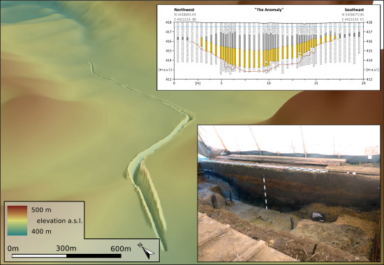
2.2.5. Direct Push Sensing
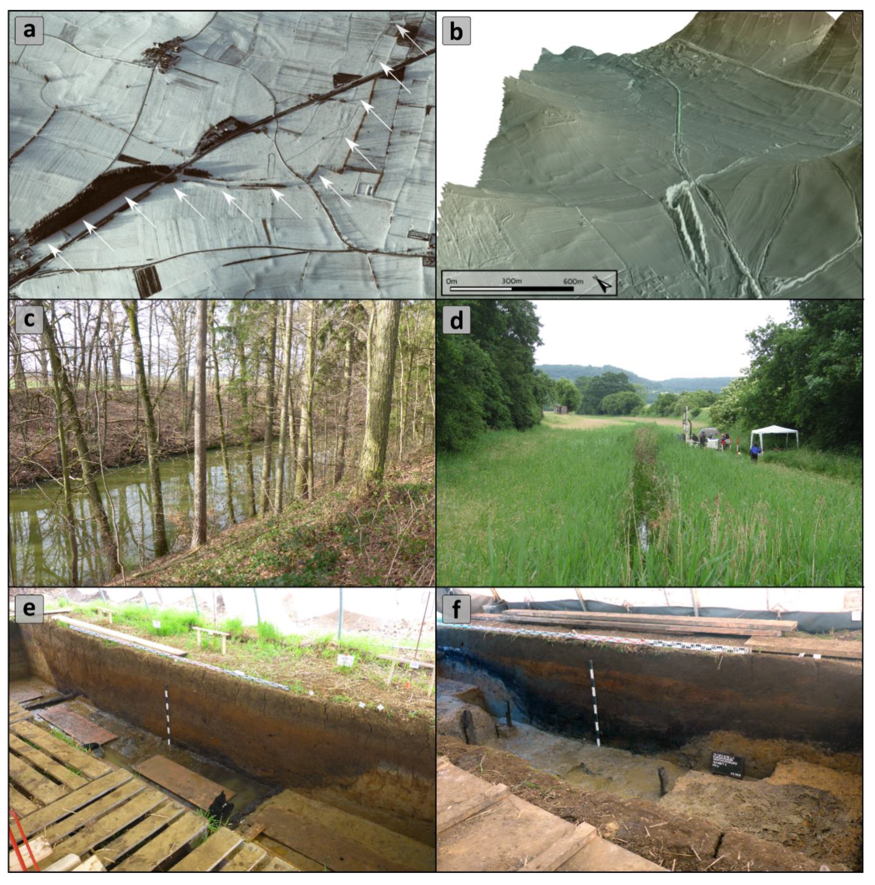
2.2.6. Archaeological Excavations
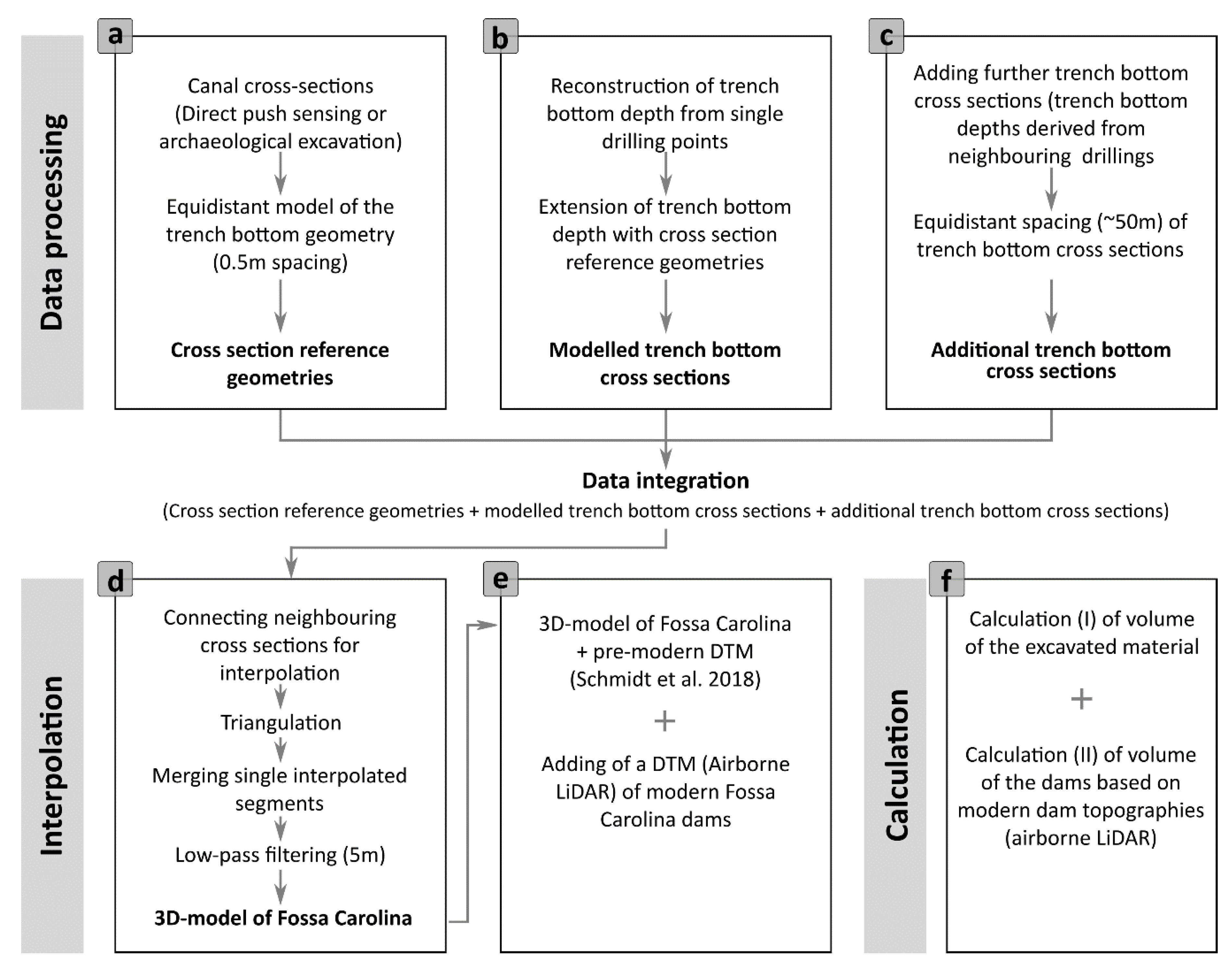
2.3. Modelling Routine
3. Results
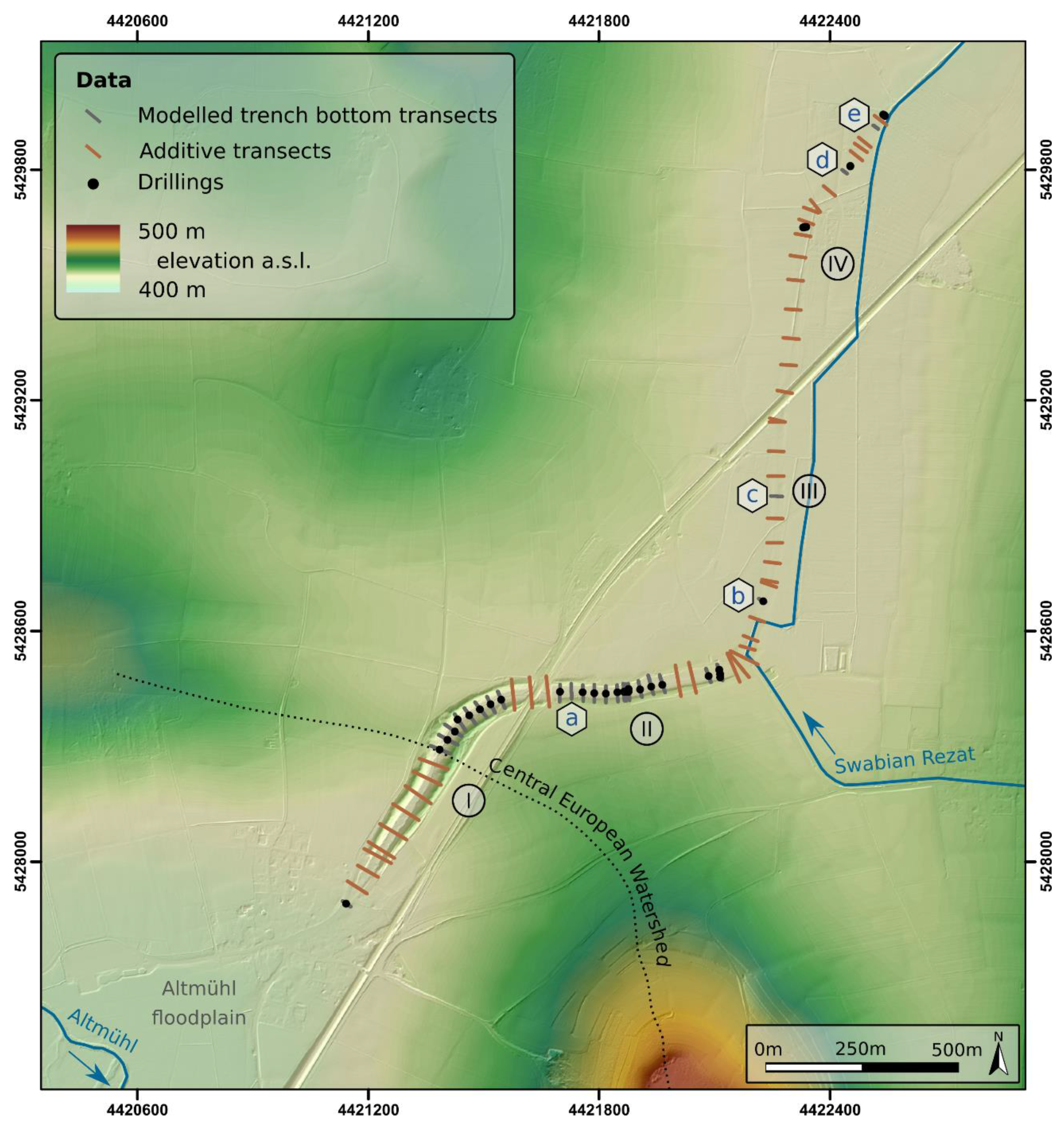
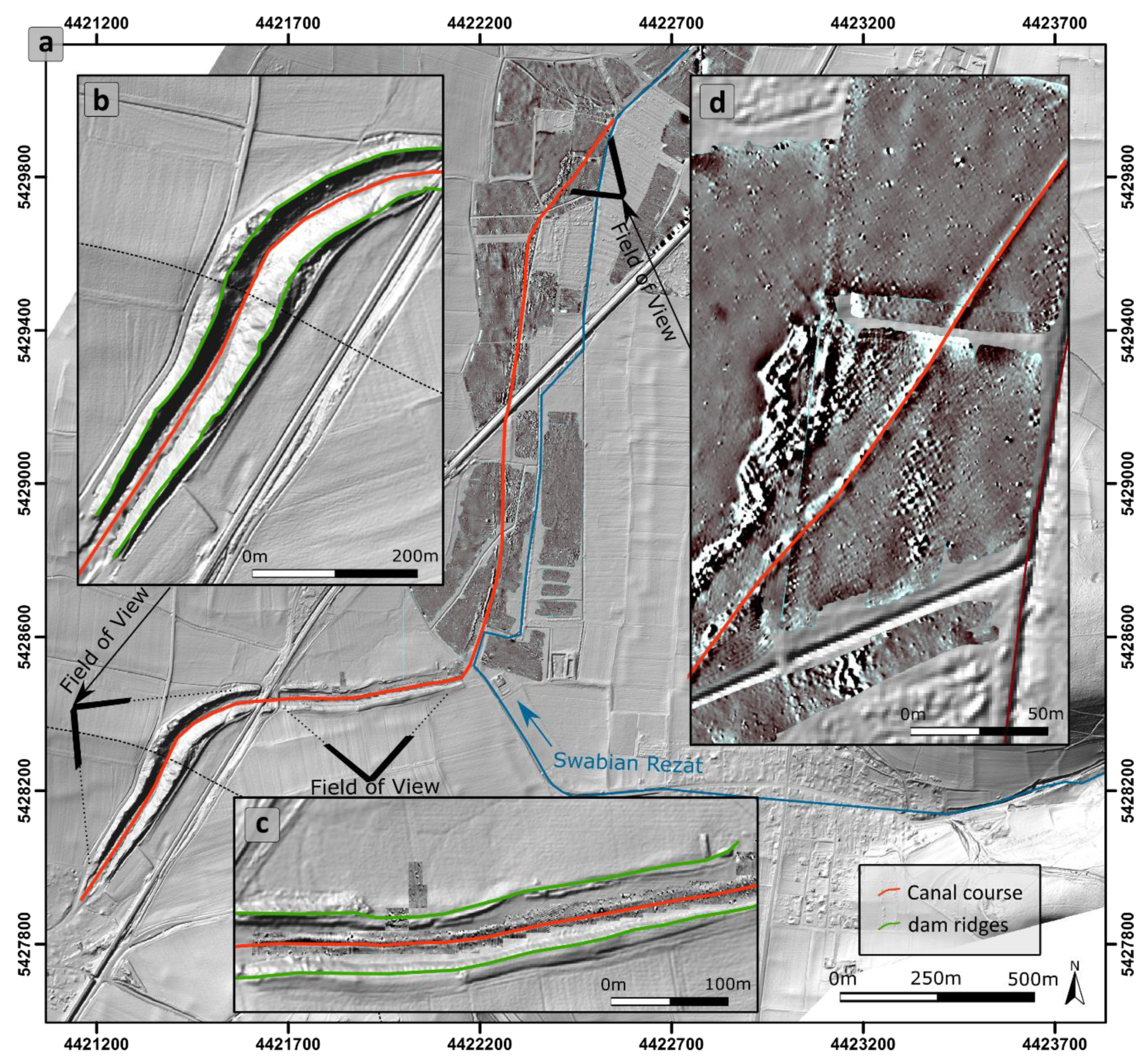
3.1. Canal Course
3.2. Cross-Section Reference Geometries
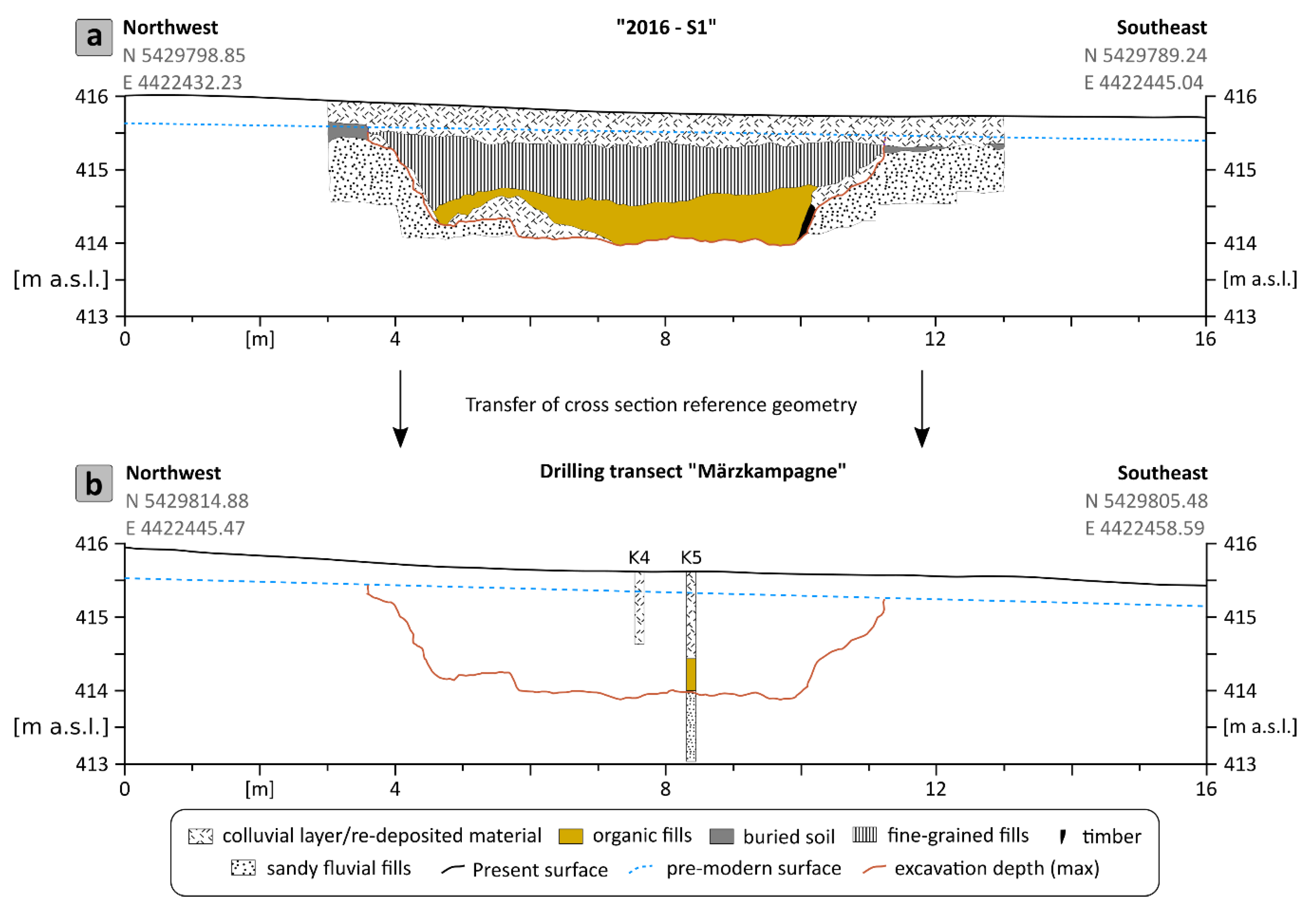
3.3. Application of Cross-Section Reference Geometries to Vibra-Coring and Additive Transects
3.4. 3D-Model
3.5. Volume Calculation
4. Discussion
4.1. 3D-Modelling Approach and Quality
4.2. The Scientific History of Fossa Carolina Volume Calculations
4.3. Where Has All the Material Gone?
5. Conclusions
Author Contributions
Funding
Acknowledgments
Conflicts of Interest
References
- McCormick, M. The Origin of the European Economy. Communications and Commerce A.D. 300–900; Cambridge University Press: Cambridge, UK, 2010. [Google Scholar]
- Squatriti, P. Digging Ditches in Early Medieval Europe. Past Present 2002, 176, 11–65. [Google Scholar] [CrossRef]
- Leitholdt, E.; Zielhofer, C.; Berg-Hobohm, S.; Schnabl, K.; Kopecky-Hermanns, B.; Bussmann, J.; Härtling, J.W.; Reicherter, K.; Unger, K. Fossa Carolina: The First Attempt to Bridge the Central European Watershed—A Review, New Findings, and Geoarchaeological Challenges. Geoarchaeology 2012, 27, 88–104. [Google Scholar] [CrossRef]
- Werther, L.; Kröger, L.; Kirchner, A.; Zielhofer, C.; Leitholdt, E.; Schneider, M.; Linzen, S.; Berg-Hobohm, S.; Ettel, P. Fossata Magna—A Canal Contribution to Harbour Construction in the 1st Millenium AD. In Harbours as Object of Interdisciplinary Research: Archaeology + History + Geosciences; Carnap-Bornheim, C.V., Daim, F., Ettel, P., Warnke, U., Eds.; Verl. des RGZM: Mainz, Germany, 2018; pp. 355–372. ISBN 9783884672839. [Google Scholar]
- Preiser-Kapeller, J.; Werther, L. Connecting Harbours: A Comparison of Traffic Networks across Ancient and Medieval Europe. In Harbours as Object of Interdisciplinary Research: Archaeology + History + Geosciences; Carnap-Bornheim, C.V., Daim, F., Ettel, P., Warnke, U., Eds.; Verl. des RGZM: Mainz, Germany, 2018; pp. 7–31. ISBN 9783884672839. [Google Scholar]
- Beck, F. Der Karlsgraben Eine Historische, Topographische und Kritische Abhandlung. Mit Beilagen; Verlag der Friedrich Kornschen Buchhandlung: Nürnberg, Germany, 1911. [Google Scholar]
- Berg-Hobohm, S. Archäologische Forschungsgeschichte der Fossa Carolina. In Großbaustelle 793: Das Kanalprojekt Karls des Großen zwischen Rhein und Donau; Ettel, P., Berg-Hobohm, S., Eds.; Verl. des Römisch-Germanischen Zentralmuseums: Mainz, Germany, 2014; pp. 1–4. ISBN 978-3-88467-232-7. [Google Scholar]
- Koch, R. Fossa Carolina—1200 Jahre Karlsgraben; Denkmalpflege Informationen: München, Germany, 1993. [Google Scholar]
- Koch, R. Neue Beobachtungen und Forschungen zum Karlsgraben. Jahrbuch des Historischen Vereins für Mittelfranken 1996, 97, 1–16. [Google Scholar]
- Birzer, F. Der Kanalbauversuch Karls des Großen. Geologische Blätter für Nordost-Bayern und Angrenzende Gebiete 1958, 8, 171–178. [Google Scholar]
- Bruno, F.; Bruno, S.; de Sensi, G.; Luchi, M.-L.; Mancuso, S.; Muzzupappa, M. From 3D reconstruction to virtual reality: A complete methodology for digital archaeological exhibition. J. Cult. Herit. 2010, 11, 42–49. [Google Scholar] [CrossRef]
- De Reu, J.; de Smedt, P.; Herremans, D.; van Meirvenne, M.; Laloo, P.; de Clercq, W. On introducing an image-based 3D reconstruction method in archaeological excavation practice. J. Archaeol. Sci. 2014, 41, 251–262. [Google Scholar] [CrossRef]
- Ducke, B.; Score, D.; Reeves, J. Multiview 3D reconstruction of the archaeological site at Weymouth from image series. Comput. Graph. 2011, 35, 375–382. [Google Scholar] [CrossRef]
- Richards-Rissetto, H. What can GIS + 3D mean for landscape archaeology? J. Archaeol. Sci. 2017, 84, 10–21. [Google Scholar] [CrossRef] [Green Version]
- Forte, M. Virtual Reality, Cyberarchaeoloogy, teleimmersive Archaeology. In 3D Recording and Modelling in Archaeology and Cultural Heritage: Theory and Best Practises; Remondino, F., Campana, S., Eds.; Archaeopress: Oxford, UK, 2014; pp. 113–127. [Google Scholar]
- Koutsoudis, A.; Arnaoutoglou, F.; Chamzas, C. On 3D reconstruction of the old city of Xanthi. A minimum budget approach to virtual touring based on photogrammetry. J. Cult. Herit. 2007, 8, 26–31. [Google Scholar] [CrossRef]
- Pickett, J.; Schreck, J.S.; Holod, R.; Rassamakin, Y.; Halenko, O.; Woodfin, W. Architectural energetics for tumuli construction: The case of the medieval Chungul Kurgan on the Eurasian steppe. J. Archaeol. Sci. 2016, 75, 101–114. [Google Scholar] [CrossRef]
- Lacquement, C.H. Recalculating mound volume at moundville. Southeast. Archaeol. 2010, 29, 341–354. [Google Scholar] [CrossRef]
- Sherwood, S.C.; Kidder, T.R. The DaVincis of dirt: Geoarchaeological perspectives on Native American mound building in the Mississippi River basin. J. Anthropol. Archaeol. 2011, 30, 69–87. [Google Scholar] [CrossRef]
- Zielhofer, C.; Wellbrock, K.; Al-Souliman, A.S.; von Grafenstein, M.; Schneider, B.; Fitzsimmons, K.; Stele, A.; Lauer, T.; Von Suchodoletz, H.; Grottker, M. Climate forcing and shifts in water management on the Northwest Arabian Peninsula (mid-Holocene Rasif wetlands, Saudi Arabia). Quat. Int. 2018, 473, 120–140. [Google Scholar] [CrossRef]
- Grammer, B.; Draganits, E.; Gretscher, M.; Muss, U. LiDAR-guided Archaeological Survey of a Mediterranean Landscape: Lessons from the Ancient Greek Polis of Kolophon (Ionia, Western Anatolia). Archaeol. Prospect. 2017, 54, 64. [Google Scholar] [CrossRef]
- Cowley, D.; Moriarty, C.; Geddes, G.; Brown, G.; Wade, T.; Nichol, C. UAVs in Context: Archaeological Airborne Recording in a National Body of Survey and Record. Drones 2018, 2, 2. [Google Scholar] [CrossRef]
- Andersen, N.H. The Sarup Enclosures. The Funnel Beaker Culture of the Sarup Site including Two Causewaysed Camps Compared to the Contemporary Settlements in the Area and other European Enclosures; Aarhus University Press: Aarhus, Denmark, 1997. [Google Scholar]
- De Smedt, P.; van Meirvenne, M.; Herremans, D.; de Reu, J.; Saey, T.; Meerschman, E.; Crombé, P.; de Clercq, W. The 3-D reconstruction of medieval wetland reclamation through electromagnetic induction survey. Sci. Rep. 2013, 3, 1517. [Google Scholar] [CrossRef]
- De Smedt, P.; van Meirvenne, M.; Meerschman, E.; Saey, T.; Bats, M.; Court-Picon, M.; de Reu, J.; Zwertvaegher, A.; Antrop, M.; Bourgeois, J.; et al. Reconstructing palaeochannel morphology with a mobile multicoil electromagnetic induction sensor. Geomorphology 2011, 130, 136–141. [Google Scholar] [CrossRef]
- Diamanti, N.G.; Tsokas, G.N.; Tsourlos, P.I.; Vafidis, A. Integrated interpretation of geophysical data in the archaeological site of Europos (northern Greece). Archaeol. Prospect. 2005, 12, 79–91. [Google Scholar] [CrossRef]
- Hausmann, J.; Zielhofer, C.; Werther, L.; Berg-Hobohm, S.; Dietrich, P.; Heymann, R.; Werban, U. Direct push sensing in wetland (geo)archaeology: High-resolution reconstruction of buried canal structures (Fossa Carolina, Germany). Quat. Int. 2017, 473, 21–36. [Google Scholar] [CrossRef]
- Hadler, H.; Vött, A.; Newig, J.; Emde, K.; Finkler, C.; Fischer, P.; Willershäuser, T. Geoarchaeological evidence of marshland destruction in the area of Rungholt, present-day Wadden Sea around Hallig Südfall (North Frisia, Germany), by the Grote Mandrenke in 1362 AD. Quat. Int. 2018, 473, 37–54. [Google Scholar] [CrossRef]
- Seeliger, M.; Pint, A.; Frenzel, P.; Weisenseel, P.; Erkul, E.; Wilken, D.; Wunderlich, T.; Başaran, S.; Bücherl, H.; Herbrecht, M. Using a Multi-Proxy Approach to Detect and Date a Buried part of the Hellenistic City Wall of Ainos (NW Turkey). Geosciences 2018, 8, 357. [Google Scholar] [CrossRef]
- Canti, M.; Huisman, D.J. Scientific advances in geoarchaeology during the last twenty years. J. Archaeol. Sci. 2015, 56, 96–108. [Google Scholar] [CrossRef] [Green Version]
- Beuzen-Waller, T.; Stock, F.; Kondo, Y. Geoarchaeology: A toolbox for revealing latent data in sedimentological and archaeological records. Quat. Int. 2018, 483, 1–4. [Google Scholar] [CrossRef]
- Zielhofer, C.; Leitholdt, E.; Werther, L.; Stele, A.; Bussmann, J.; Linzen, S.; Schneider, M.; Meyer, C.; Berg-Hobohm, S.; Ettel, P. Charlemagne’s summit canal: An early medieval hydro-engineering project for passing the Central European Watershed. PLoS ONE 2014, 9, e108194. [Google Scholar] [CrossRef] [PubMed]
- Werther, L.; Feiner, D. Der Karlsgraben im Fokus der Archäologie. In Großbaustelle 793: Das Kanalprojekt Karls des Großen Zwischen Rhein und Donau; Ettel, P., Berg-Hobohm, S., Eds.; Verl. des Römisch-Germanischen Zentralmuseums: Mainz, Germany, 2014; pp. 33–40. ISBN 978-3-88467-232-7. [Google Scholar]
- Schmidt, J.; Werther, L.; Zielhofer, C. Shaping pre-modern digital terrain models: The former topography at Charlemagne’s canal construction site. PLoS ONE 2018, 13, e0200167. [Google Scholar] [CrossRef] [PubMed]
- Zielhofer, C.; Rabbel, W.; Wunderlich, T.; Vött, A.; Berg, S. Integrated geophysical and (geo)archaeological explorations in wetlands. Quat. Int. 2018, 473, 1–2. [Google Scholar] [CrossRef]
- Werther, L.; Zielhofer, C.; Herzig, F.; Leitholdt, E.; Schneider, M.; Linzen, S.; Berg-Hobohm, S.; Ettel, P.; Kirchner, A.; Dunkel, S. Häfen verbinden. Neue Befunde zu Verlauf, wasserbaulichem Konzept und Verlandung des Karlsgrabens. In Häfen im 1. Millennium AD: Bauliche Konzepte, Herrschaftliche und Religiöse Einflüsse, 1st ed.; Schmidts, T., Vučetić, M.M., Eds.; Schnell & Steiner; Verl. des RGZM: Regensburg, Mainz, Germany, 2015; pp. 151–185. ISBN 978-3-7954-3039-9. [Google Scholar]
- Werther, L. Karlsgraben doch Schiffbar? Aktuelles aus der Landesarchäologie. Archäologie Deutschland 2017, 5, 41–42. [Google Scholar]
- Völlmer, J.; Zielhofer, C.; Hausmann, J.; Dietrich, P.; Werban, U.; Schmidt, J.; Werther, L.; Berg, S. Minimalinvasive Direct-push Erkundung in der Feuchtboden(geo)archäologie am Beispiel des Karlsgrabens (Fossa Carolina). Archäologisches Korrespondenzblatt 2018, 48, 577–593. [Google Scholar]
- Leitholdt, E.; Krüger, A.; Zielhofer, C. The medieval peat layer of the Fossa Carolina—Evidence for bridging the Central European Watershed or climate control? Z. Geomorphol. Suppl. Issues 2014, 58, 189–209. [Google Scholar] [CrossRef]
- Kirchner, A.; Zielhofer, C.; Werther, L.; Schneider, M.; Linzen, S.; Wilken, D.; Wunderlich, T.; Rabbel, W.; Meyer, C.; Schmidt, J.; et al. A multidisciplinary approach in wetland geoarchaeology: Survey of the missing southern canal connection of the Fossa Carolina (SW Germany). Quat. Int. 2018, 473, 3–20. [Google Scholar] [CrossRef]
- Schmidt-Kaler, H. Geologie und Landschaftsentwicklung im Rezat-Altmühl Bereich; Bau intern Special Issue; Lipp: München, Germany, 1993; pp. 8–10. [Google Scholar]
- Zielhofer, C.; Kirchner, A. Naturräumliche Gunstlage der Fossa Carolina. In Großbaustelle 793: Das Kanalprojekt Karls des Großen zwischen Rhein und Donau; Ettel, P., Berg-Hobohm, S., Eds.; Verl. des Römisch-Germanischen Zentralmuseums: Mainz, Germany, 2014; pp. 5–8. ISBN 978-3-88467-232-7. [Google Scholar]
- Bavarian State Department of Cultural Heritage BLfD.; Luftbildarchiv, Archivnummer: 7130_027, Filmnummer: 3840B, Bild 12, 19.02.1985, 1985. Available online: https://www.ldbv.bayern.de/vermessung/luftbilder/archiv.html (accessed on 13 May 2013).
- Bavarian Land Surveying Office. Geländemodell. 2018. Available online: https://www.ldbv.bayern.de/produkte/3dprodukte/gelaende.html (accessed on 12 April 2019).
- Bavarian Land Surveying Office. Airborne Laserscanning. 2018. Available online: https://www.ldbv.bayern.de/produkte/3dprodukte/laser.html (accessed on 12 April 2019).
- Linzen, S.; Schultze, V.; Chwala, A.; Schüler, T.; Schulz, M.; Stolz, R.; Meyer, H.-G. Quantum Detection Meets Archaeology—Magnetic Prospection with SQUIDs, Highly Sensitive and Fast. In New Technologies for Archaeology; Reindel, M., Wagner, G.A., Eds.; Springer: Berlin/Heidelberg, Germany, 2009; pp. 71–85. [Google Scholar]
- Schneider, M.; Stolz, R.; Linzen, S.; Schiffler, M.; Chwala, A.; Schulz, M.; Dunkel, S.; Meyer, H.-G. Inversion of geo-magnetic full-tensor gradiometer data. J. Appl. Geophys. 2013, 92, 57–67. [Google Scholar] [CrossRef]
- Linzen, S.; Schneider, M.; Berg-Hobohm, S.; Werther, L.; Ettel, P.; Zielhofer, C.; Schmidt, J.; Fassbinder, J.W.E.; Wilken, D.; Fediuk, A.; et al. From magnetic SQUID prospection to excavation—Investigations at Fossa Carolina, Germany. In Proceedings of the 12th International Conference of Archaeoloigcal Prospection, Bradford, UK, 12–16 September 2017; Jennings, B., Gaffney, C., Sparrow, T., Gaffney, S., Eds.; Archaeopress: Oxford, UK, 2017; pp. 144–145, ISBN 978 1 78491 677 0. [Google Scholar]
- Linzen, S.; Schneider, M. Der Karlsgraben im Fokus der Geophysik. In Großbaustelle 793: Das Kanalprojekt Karls des Großen zwischen Rhein und Donau; Ettel, P., Berg-Hobohm, S., Eds.; Verl. des Römisch-Germanischen Zentralmuseums: Mainz, Germany, 2014; pp. 29–32. ISBN 978-3-88467-232-7. [Google Scholar]
- Dietrich, P.; Leven, C. Direct Push-Technologies. In Groundwater Geophysics, 2nd ed.; Kirsch, R., Ed.; Springer: Berlin, Germany, 2009; pp. 347–366. [Google Scholar]
- Leven, C.; Weiß, H.; Vienken, T.; Dietrich, P. Direct-Push-Technologien—Effiziente Untersuchungsmethoden für die Untergrunderkundung. Grundwasser 2011, 16, 221–234. [Google Scholar] [CrossRef]
- Hausmann, J.; Dietrich, P.; Vienken, T.; Werban, U. Technique, analysis routines, and application of direct push-driven in situ color logging. Environ. Earth Sci. 2016, 75, 659. [Google Scholar] [CrossRef]
- Butler, J.J.; Healey, J.M.; Zheng, L.; McCall, G.W.; Schulmeister, M.K. Hydrostratigraphic Characterization of Unconsolidated Alluvial Deposits with Direct-Push Sensor Technology; Kansas Geological Survey Open-File report 99-40; University of Kansas Field Station: Lawrence, KS, USA, 1999. [Google Scholar]
- Schulmeister, M.K.; Butler, J.J.; Healey, J.M.; Zheng, L.; Wysocki, D.A.; McCall, G.W. Direct-Push Electrical Conductivity Logging for High-Resolution Hydrostratigraphic Characterization. Groundw. Monit. Remediat. 2003, 23, 52–62. [Google Scholar] [CrossRef]
- Davis, J.C.; Herzfeld, U.C. Computers in Geology. 25 Years of Progress; Oxford University Press: New York, NY, USA, 1993; ISBN 0195085930. [Google Scholar]
- Carey, C.; Howard, A.J.; Knight, D.; Corcoran, J.; Heathcote, J. Deposit Modelling and Archaeology; University of Brighton: Brighton, UK, 2018; ISBN 978-1-5272-2244-1. [Google Scholar]
- Earley-Spadoni, T. Spatial History, deep mapping and digital storytelling: Archaeology’s future imagined through an engagement with the Digital Humanities. J. Archaeol. Sci. 2017, 84, 95–102. [Google Scholar] [CrossRef]
- Chapman, H.; Adcock, J.; Gater, J. An approach to mapping buried prehistoric palaeosols of the Atlantic seaboard in Northwest Europe using GPR, geoarchaeology and GIS and the implications for heritage management. J. Archaeol. Sci. 2009, 36, 2308–2313. [Google Scholar] [CrossRef]
- McCoy, M.D. Geospatial Big Data and archaeology: Prospects and problems too great to ignore. J. Archaeol. Sci. 2017, 84, 74–94. [Google Scholar] [CrossRef]
- Hofmann, H.H. Kaiser Karls Kanalbau: “Wie Künig Carl der Grosse unterstünde die Donaw vnd den Rhein zusam̄enzugraben”, 2nd ed.; Thorbecke: Sigmaringen, Germany, 1976; ISBN 3-7995-4014-8. [Google Scholar]
- Berg-Hobohm, S.; Werther, L. Das rezente Erscheinungsbild des Karlsgrabens. In Großbaustelle 793: Das Kanalprojekt Karls des Großen Zwischen Rhein und Donau; Ettel, P., Berg-Hobohm, S., Eds.; Verl. des Römisch-Germanischen Zentralmuseums: Mainz, Germany, 2014; pp. 9–12. ISBN 978-3-88467-232-7. [Google Scholar]


| Technique | Number | Name (Label in Figure 2) | References | Depth Accuracy | Lateral Distances | Scale | Resolution of Stratigraphy | Pace |
|---|---|---|---|---|---|---|---|---|
| Excavation | 3 trenches | “2013” (c) “2016–S1” (d) “2016–S2” (e) | Werther and Feiner 2014 [33]; Werther et al. 2015 [36]; Werther 2017 [37] | ++ | cm-scale | micro to small | +++ | - |
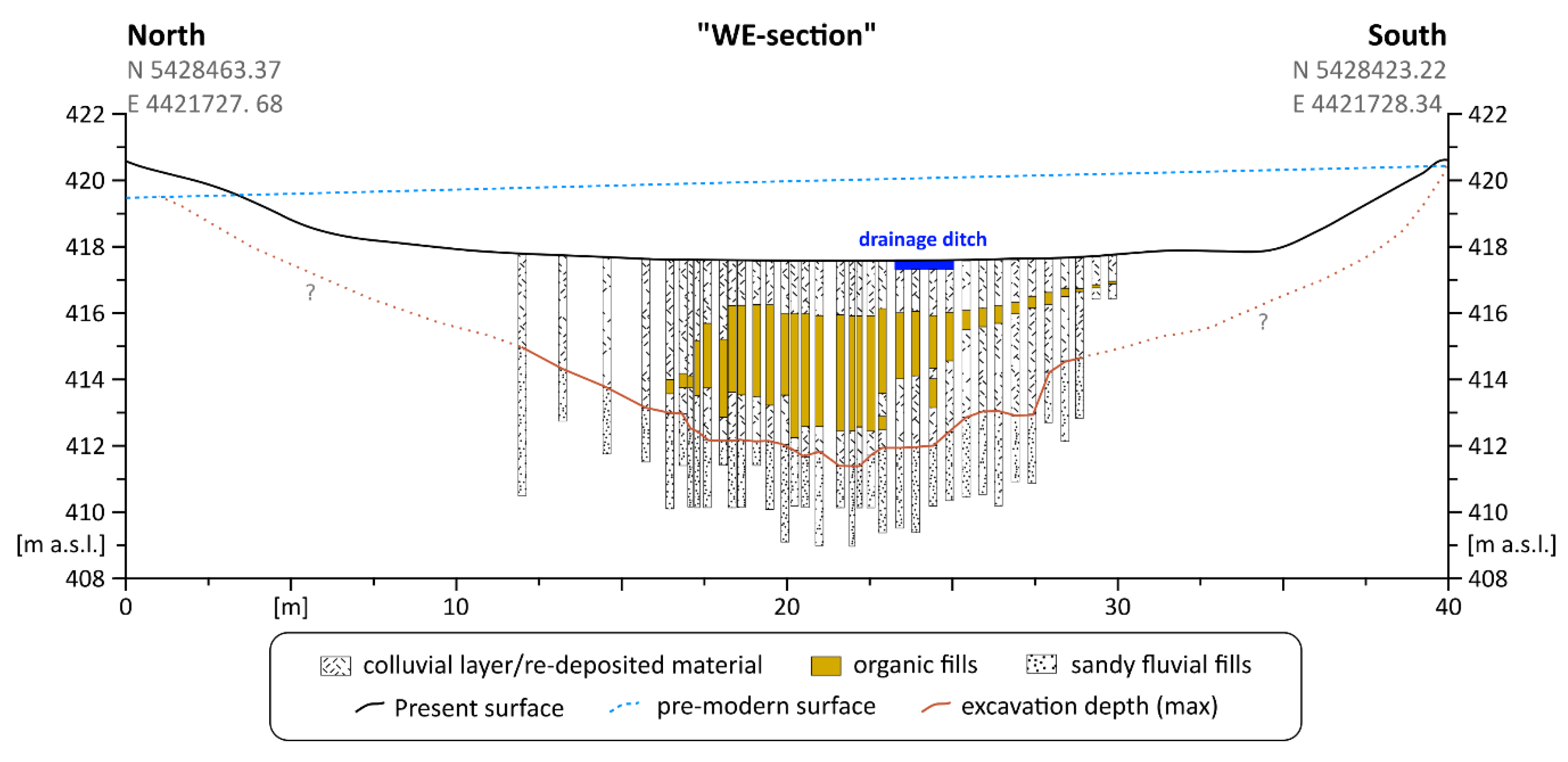
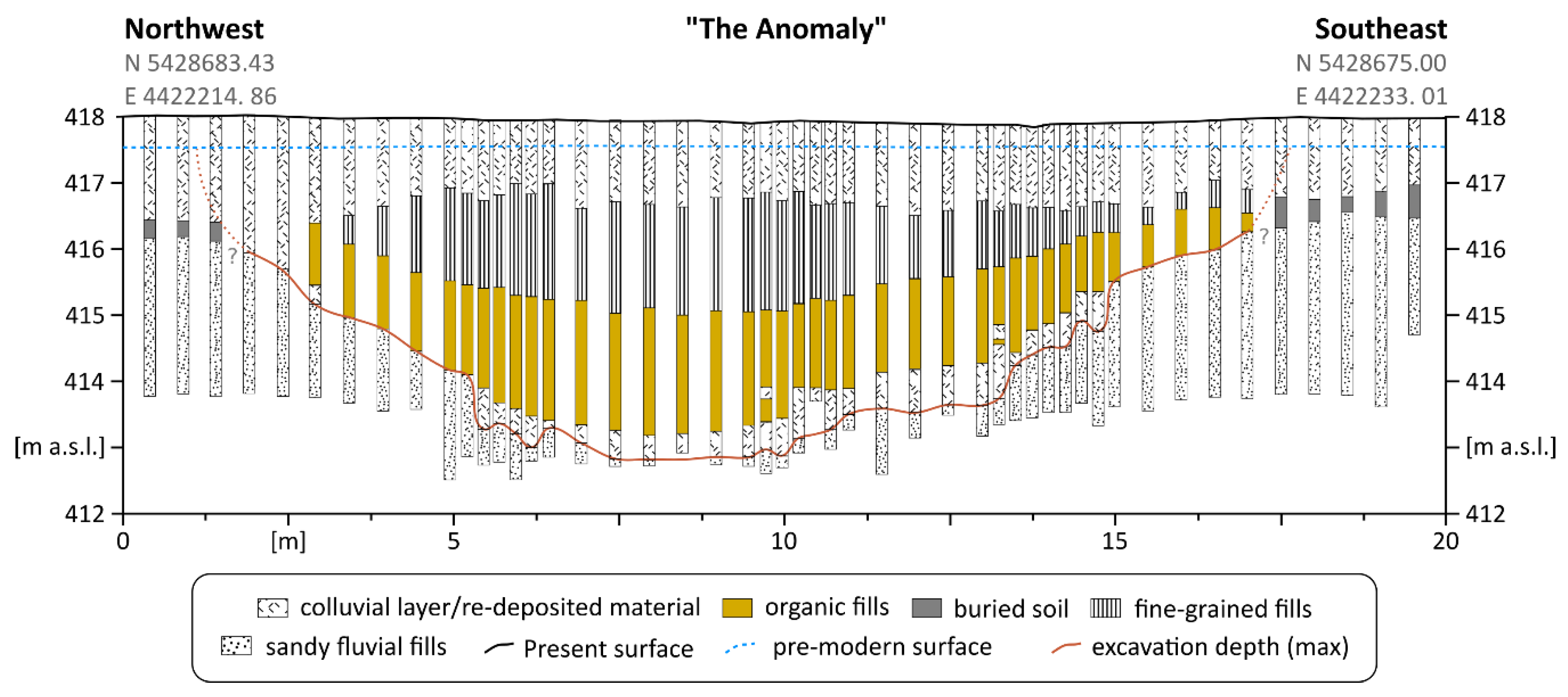
| Direct-push | 2 transects | “WE-Section” (a) “TheAnomaly” (b) | Völlmer et al. 2019 [38]; This study | ++ | 12.5 to 50 cm | micro to medium | ++ | ++ |
| Drilling | 26 transects | - | Leitholdt et al. 2012 [3]; Leitholdt et al. 2014 [39]; Zielhofer et al. 2014 [32]; Kirchner et al. 2018 [40]; This study | ○ | Up to 1 m | small to medium | + | + |
| Fossa Carolina Section | Length (m) | Cross-Section Reference Geometry | Type | Transferred to n Core Positions |
|---|---|---|---|---|
| Central Section | 803 | “WE cross-section” | direct push sensing | 10 |
| WE Section | 494 | “WE cross-section” | direct push sensing | 16 |
| Northern Section I (S) | 368 | “The Anomaly” | direct push sensing | 1 |
| Northern Section II (N) | 370 | “2013” | archaeological excavation | 6 |
| North-Eastern Section I (S) | 476 | “2013” | archaeological excavation | 0 |
| North-Eastern Section II (M) | 198 | “2016–S1” | archaeological excavation | 2 |
| North-Eastern Section III (N) | 120 | “2016–S2” | archaeological excavation | 4 |
| No. | Study | Volume | Object | Method | Comments |
|---|---|---|---|---|---|
| 1 | Birzer 1958 [10] | 80,000 m3 | canal trench | estimation/calculation | minimum; only Central and WE-Section |
| 3 | Birzer 1958 [10] | 450,000 m3 | canal trench | estimation/calculation | Assumed canal length of 4.5 km and constant trench bottom level |
| 6 | Hofmann 1976 [60] | 130,000 m3 | canal trench | calculation | Assumed canal length 1.4 km, width 30 m, depth 6 m |
| 5 | Koch 1993 [8] | several 100,000 m3 | canal trench | estimation | Assumed canal length 5–7 km |
| 2 | This study | 297,667 m3 | canal trench | calculation | Integrative approach |
| 7 | This study | 119,681 m3 | dams | calculation | Calculated based on present dams in comparison to pre-modern DTM |
| Section | Section Length | Length Proportion | Trench Volume | Trench Volume Proportion | Dam Volume | Ratio Dams/Trench |
|---|---|---|---|---|---|---|
| Total | 2829 m | 100% | 297,667 m3 | 100% | 119,681 m3 | 40% |
| Central Section | 803 m | 28% | 160,815 m3 | 54% | 83,826 m3 | 52% |
| WE Section | 494 m | 17% | 96,496 m3 | 32% | 20,449 m3 | 21% |
| Northern Section | 738 m | 27% | 26,267 m3 | 9% | 10,864 m3 | 41% |
| North-Eastern Section | 794 m | 27% | 14,088 m3 | 5% | 4,558 m3 | 32% |
© 2019 by the authors. Licensee MDPI, Basel, Switzerland. This article is an open access article distributed under the terms and conditions of the Creative Commons Attribution (CC BY) license (http://creativecommons.org/licenses/by/4.0/).
Share and Cite
Schmidt, J.; Rabiger-Völlmer, J.; Werther, L.; Werban, U.; Dietrich, P.; Berg, S.; Ettel, P.; Linzen, S.; Stele, A.; Schneider, B.; et al. 3D-Modelling of Charlemagne’s Summit Canal (Southern Germany)—Merging Remote Sensing and Geoarchaeological Subsurface Data. Remote Sens. 2019, 11, 1111. https://0-doi-org.brum.beds.ac.uk/10.3390/rs11091111
Schmidt J, Rabiger-Völlmer J, Werther L, Werban U, Dietrich P, Berg S, Ettel P, Linzen S, Stele A, Schneider B, et al. 3D-Modelling of Charlemagne’s Summit Canal (Southern Germany)—Merging Remote Sensing and Geoarchaeological Subsurface Data. Remote Sensing. 2019; 11(9):1111. https://0-doi-org.brum.beds.ac.uk/10.3390/rs11091111
Chicago/Turabian StyleSchmidt, Johannes, Johannes Rabiger-Völlmer, Lukas Werther, Ulrike Werban, Peter Dietrich, Stefanie Berg, Peter Ettel, Sven Linzen, Andreas Stele, Birgit Schneider, and et al. 2019. "3D-Modelling of Charlemagne’s Summit Canal (Southern Germany)—Merging Remote Sensing and Geoarchaeological Subsurface Data" Remote Sensing 11, no. 9: 1111. https://0-doi-org.brum.beds.ac.uk/10.3390/rs11091111