An Effective Classification Scheme for Hyperspectral Image Based on Superpixel and Discontinuity Preserving Relaxation


College of Urban and Environment, Liaoning Normal University, Dalian 116029, China
*
Author to whom correspondence should be addressed.
Remote Sens. 2019, 11(10), 1149; https://0-doi-org.brum.beds.ac.uk/10.3390/rs11101149
Submission received: 9 April 2019
/
Revised: 6 May 2019
/
Accepted: 6 May 2019
/
Published: 14 May 2019
(This article belongs to the Section Remote Sensing Image Processing)
Abstract
:Hyperspectral image (HSI) classification is one of the most active topics in remote sensing. However, it is still a nontrivial task to classify the hyperspectral data accurately, since HSI always suffers from a large number of noise pixels, the complexity of the spatial structure of objects and the spectral similarity between different objects. In this study, an effective classification scheme for hyperspectral image based on superpixel and discontinuity preserving relaxation (DPR) is proposed to discriminate land covers of interest. A novel technique for measuring the similarity of a pair of pixels in HSI is suggested to improve the simple linear iterative clustering (SLIC) algorithm. Unlike the existing application of SLIC technique to HSI, the improved SLIC algorithm can be directly used to segment HSI into superpixels without using principal component analysis in advance, and is free of parameters. Furthermore, the proposed three-step classification scheme explores how to effectively use the global spectral information and local spatial structure of hyperspectral data for HSI classification. Compared with the existing two-step classification framework, the use of DPR technology in preprocessing significantly improves the classification accuracy. The effectiveness of the proposed method is verified on three public real hyperspectral datasets. The comparison results of several competitive methods show the superiority of this scheme.
1. Introduction
A hyperspectral image (HSI) is acquired by hyperspectral remote sensors and composed of hundreds of bands over the same spatial area. It can provide high spectral resolution and rich spatial information. These features of HSIs contain a wealth of information to identify land covers of interest effectively. As a fundamental problem, HSI classification has been paid more and more attention recently, partially due to its widely successful applications in various fields, such as precision agriculture [1], urban planning [2], environment monitoring [3], target detection [4], and anomaly detection [5].
HSI classification is to assign each pixel to a meaningful and physical class based on their spectral features and the land coverage surface. During the last decades, plenty of HSI classification methods have been proposed. Some typical approaches; for example, support a vector machine (SVM)-based method [6,7,8,9], multinomial logistic regression-based techniques [10,11], various feature selection-based methods [12,13], and sparse representation-based methods [14,15], have been demonstrated to be very successful techniques. The aforementioned methods make full use of the spectral features of hyperspectral data in the process of classification. Generally, the classification results obtained by those above-mentioned methods that do not consider the spatial information of HSI are often not ideal. To further improve the classification performance, a large number of methods combining spectral information with spatial information have been investigated in recent years [16,17,18,19,20,21,22].
Among of the spectral–spatial based approaches, some spatial filtering techniques are developed [23,24,25,26,27,28]. The purpose of applying these techniques to HSI classification is to denoise HSI in the pre-processing task or improve the classification accuracy in post-processing. Several popular methods are discontinuity preserving relaxation (DPR) [28], Markov random fields (MRF) [29,30], probabilistic relaxation (PR) [31], the local binary pattern filter [32], the edge-preserving filter [33], Gabor filter [34], the extended morphological profiles filter [35] and so on.
Although the application of spatial filtering techniques in HSI classification can effectively reduce some noise pixels and provide a better classification result, the adopted spatial region is fixed in size and shape. In other words, the spatial information of HSI may be exploited insufficiently. Recent research shows that superpixel segmentation provides a powerful way to address this problem, as a superpixel is with adaptive shape and size. According to the techniques used to generate a superpixel, the known superpixel segmentation methods can be categorized into graph-based methods [36,37,38], gradient-ascent-based methods [39,40] and cluster-based methods [41]. Among of these segmentation algorithms, simple linear iterative clustering (SLIC) algorithm seems to be more popular because it is fast to compute, simple to use and good to adhere to boundaries [41].
Over the past decade, superpixel segmentation methods have also been extended to HSI classification [42,43,44,45,46,47,48,49,50], aiming at making full use of spectral information and spatial structure in hyperspectral data. By the combination of different segmentation techniques with various classification methods, a number of approaches for HSI classification have been developed, such as ER with sparse representation [42,51,52,53], SVM [54] or extreme learning machines [55], SLIC with multi-morphological method [56], SVM [57] or convolutional neural network [58] and so on. These HSI classification methods based on superpixel segmentation display good performance in experiments. Generally, when using SLIC algorithms to segment HSI, the principal component analysis (PCA) method must be adopted previously and the first three components are taken as the Lab color space. However, it will still inevitably encounter the difficulties of selecting the optimal weight in SLIC algorithms. To address the above-mentioned problems, therefore, it is necessary to improve SLIC used in color image segmentation so that it can be directly applied to segment HSI.
In this study, a novel technique to measure the similarity of a pair of pixels in HSI is suggested. The proposed similarity is designed especially for the SLIC algorithm so that SLIC can be used to segment HSI directly without adopting PCA in advance. The advantages of the proposal lie in: on the one hand, we can better measure the similarity between two pixels since the spectral distance, spectral correlation and spatial distance are considered simultaneously; on the other hand, it cleverly avoids the problem of optimal parameter setting in SLIC.
In addition, the acquired HSIs contain a large number of noise data for a variety of reasons. There is no doubt that the presence of a multiple of noise will seriously affect the accurate classification and interpretation of HSIs. Furthermore, the high-dimensional and big data features of HSI also bring great difficulties to the accurate classification of land cover. Therefore, it is very urgent and important to put forward effective methods to tackle the above-mentioned problems in the field of remote sensing. Based on the improved SLIC algorithm and DPR strategy, this study develops an effective semi-supervised HSI classification scheme. The DPR method is adopted to preserve the class boundary information well in the process of denoising. In post-processing, the use of the superpixels with adaptive shape and size can effectively improve the classification accuracy.
The main contributions of the proposal are summarized as follows.
- An effective classification scheme for HSI is developed based on DPR strategy, SVM and the improved SLIC method.
- A novel technique to measure the similarity of a pair of pixels in HSI is proposed to improve the SLIC algorithm.
- The improved SLIC algorithm can be directly applied to superpixel segmentation of hyperspectral data and is free of parameters.
2. The Proposed Classification Scheme for HSI
We first introduce some notations used in this study.
Let be a hyperspectral image with n pixels; indicate the spectral vector with regard to the pixel xi; B is the number of bands.
denotes a set of spatial neighbors of the pixel xi. We herein adopt the Moore neighbor, which is defined as
where ) is the spatial coordinate of the pixel xi.
2.1. Discontinuity Preserving Relaxation
In hyperspectral data, it is possible that the same class ground objects are with different spectra and the same spectrum may be corresponding to different ground objects. This feature of HSI leads to a lot of noise pixels. In addition, the acquired spectral reflectance values are also affected by water vapor and atmospheric radiation, also resulting in noisy pixels that remain despite the atmospheric compensation step. Noise pixels in hyperspectral data will obviously affect the final classification accuracy. One of the effective ways to solve this problem is to denoise hyperspectral data by using a fixed size moving window technique. The use of this technique will make smooth areas smoother and smoother, but at the same time, it blurs the boundary of the class. Fortunately, the DPR method provides a good solution to this problem, due to the fact that the DPR method preserves the class boundary information well while de-noising.
In HSI preprocessing, DPR, initially developed by Li et al. [28], adopts the local spatial relation among adjacent pixels to denoise the hyperspectral data, and attempts to preserve the class boundary information as much as possible. It is in fact an iterative relaxation procedure.
Specifically, the DPR method can be depicted as follows.
For a given HSI, let , ; is the probability of pixel xi belonging to the j-th class. The probability matrix , can be obtained by solving the following optimization problem
where is a weight to balance the first term and the second term in Equation (2); is a value of the pixel xj of the edge image. is calculated by Equation (3)
where Sobel() represents the Sobel filter that detects the discontinuities in a band image. bi denotes the i-th band of the original hyperspectral data cube.
Our earlier work [59] showed that using Roberts cross operator instead of Sobel filter operator in Equation (3) can provide better relaxation effect. The reason of doing so is that Roberts cross operator is simple, easy to calculate, and more accurate to find the class boundary information. Thus, in this study, we still use the Roberts cross operator in Equation (3), and experimental results confirm the effectiveness of this substitution again.
While applying DPR in preprocessing stage, appropriate changes are to be made since it is impossible to know previously for a given HSI.
The Sobel filter is replaced by the Roberts cross operator in Equation (3), i.e.,
For each band b, we use Equation (5) to update it constantly
where is the value of the bth band of the pixel xi in the t-th iteration.
The update process will terminate if Equation (6) is satisfied
where indicates the b-th band image; is a predetermined threshold.
2.2. Superpixel Segmentation
The superpixel algorithm partitions an image into small non-overlapping homogeneous regions with adaptive shape and size. Previous works show that superpixel segmentation has achieved great success in computer vision and image analysis. Among of the popular superpixel algorithms, the simple linear iterative cluster (SLIC) [41] is a more powerful method because of its advantages of simple use, fast computing and better preservation of the class boundary. SLIC adopts the k-means cluster technique to segment an image according to the spatial structure and color.
The distance between two pixels is defined as follows,
where dc and ds denote the color distance and spatial distance of a pair of pixels, respectively; Nc is the maximum color distance; s is the segmentation scale.
As pointed out in [41], determining the maximum color distance Nc is nontrivial as color distances can vary significantly from cluster to cluster and image to image. To tackle this problem, the authors fixed Nc to a constant m and rewrote Equation (7) in the following form
where m is a weight balancing color similarity and spatial proximity.
2.3. The Improved SLIC Algorithm
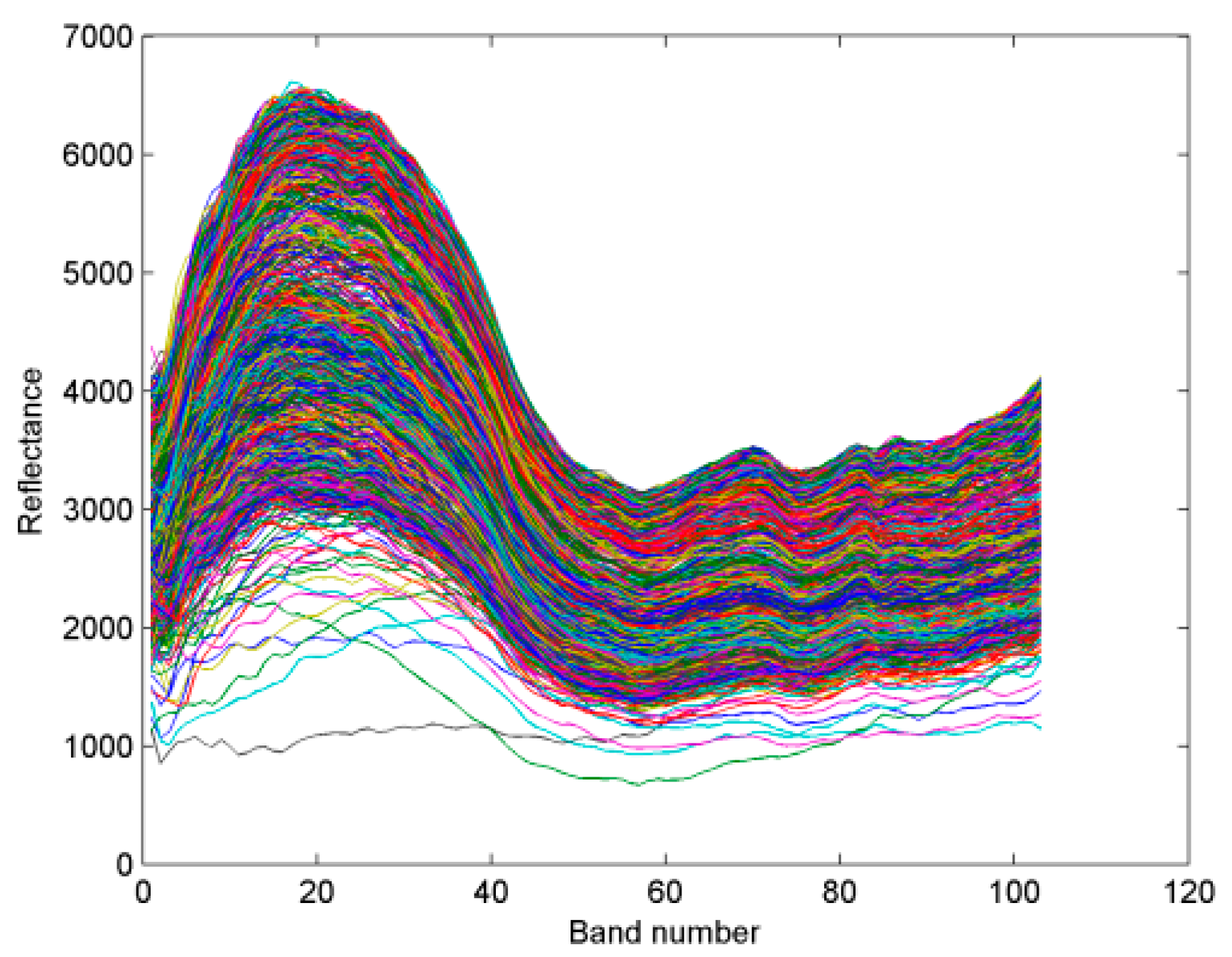
In SLIC method, the segmentation effect of HSI obviously depends on the choice of the weight m. In general, it is inappropriate to use the SLIC algorithm and the suggested parameter value directly in superpixel segmentation of HSI, as significant differences in reflectance among hundreds of bands would result in a tremendous difference between spectral distance and spatial distance. In addition, it can be seen from Figure 1 that even for two pixels in the same class, there still is a distinctive difference in spectral distance if only Euclidean distance is adopted. This obviously increases the possibility of misclassification in hyperspectral data processing.
To address the aforementioned problem, a novel technique to measure the similarity of a pair of pixels in HSI is suggested, aiming at applying SLIC algorithm handily in superpixel segmentation of HSI.
The spectral distance dspec, the spatial distance dspat and the correlation coefficient are defined as follows.
The Manhatten distance is adopted in the calculation of spectral distance in Equation (9). The value of is obvious in the range [0,1] as all components of xi and xj are positive.
For the convenience of narration, we define in the following form:
The proposed strategy to measure the similarity of a pair of pixels in HSI is as follows.
Suppose that there are k cluster centroids, c1, c2, …, ck, around the tested pixel xi. By using Equations (9), (10) and (12), the spectral distance dspec(xi, cj), the spatial distance dspat(xi, cj) and from xi to cj (j=1, 2, …, k) is calculated, respectively. In each group, we rank them in ascending order, i.e.,
where , and is a permutation of , respectively.
The tested pixel xi will be assigned to j-th cluster, if among of dspec (xi, cj), dspat(xi, cj) and , at least two of them are the smallest in the corresponding groups. Otherwise, spatial distance is considered only.
This strategy can be thought of as the generalization of Equation (8). When all of them, or spectral distance and spatial distance are minimal, this is exactly the case of Equation (8). When spectral distance and are minimal, it indicates that the spectral curves of the pixel xi and centroid cj are similar both in shape and reflectance. The assignment of pixel xi to j-th cluster is propitious to enhance the homogeneity of superpixels. As for the case of dspat(xi, cj) and , it can be regarded as the supplement of the case of spectral distance and spatial distance. The difference is that they are very similar in shape, but there are some differences in their reflection values. If there is only one smallest among of dspec(), dspat() and , it is reasonable to assign pixel xi to the closest cluster according to the first law of geography.
The proposed technique not only measures the similarity between two pixels better, but also gets rid of the trouble of choosing optimal weight m in Equation (8). It is worth noting that you can choose the distance you like to calculate the spectral distance between two pixels because the comparison takes place within each group.
The improved SLIC algorithm can be summarized as follows.
- Initialize the cluster centers by sampling pixels at scale s. Move cluster center to the pixel with the lowest gradient in a neighborhood.
- Assign each pixel to the nearest cluster in a region by using Equations (9), (10) and (12) and the proposed strategy.
- Update each cluster center.
- Repeat clustering until a given threshold is met.
2.4. An Effective Classification Scheme for HSI
In what follows, an effective classification scheme for HSI is presented based on the DPR method, SVM and improved SLIC algorithm. The proposed scheme can be divided into three steps.
Step 1. Data preprocessing.
There is no doubt that a large number of noise pixels in hyperspectral data will affect the HSI classification result. In order to get a better classification result, it is very necessary to preprocess hyperspectral data before classification. In this work, we prefer to take DPR as the data preprocessing method to denoise a given HSI. Specifically, we use Equations (4)–(6) to do this work.
Step 2. Classification at pixel wise.
Previous studies have demonstrated that SVM is a more powerful classifier in machine learning and hyperspectral data analysis. In this step, SVM with five-fold cross-validation (SVM-5) is used to classify the preprocessed HSI in a pixel-wise fashion. To enhance the performance of SVM-5, the Gaussian radial basis function (RBF) kernel is taken as its kernel function. The optimization process of the parameters used in SVM-5 is implemented by means of five-fold cross-validation.
Step 3. Post-proprecessing
After data preprocessing, we have also used the improved SLIC algorithm to carry out the superpixel segmentation of HSI. The obtained superpixels are herein used to improve the classification result provided in step 2.
The superpixel segmentation of HSI is based on the assumption that the spatial adjacent pixels in the remote sensing image have similar spectral properties and, thus, should fall into the same class. This assumption allows us to apply superpiexls to the post-processing of HSI classification. Unlike the MRF method with fixed-size window, superpixels have adaptive shapes and sizes. This feature of a superpixel makes it favorable for its application in the post-processing of HSI classification. Experimental results of this study confirm this idea.
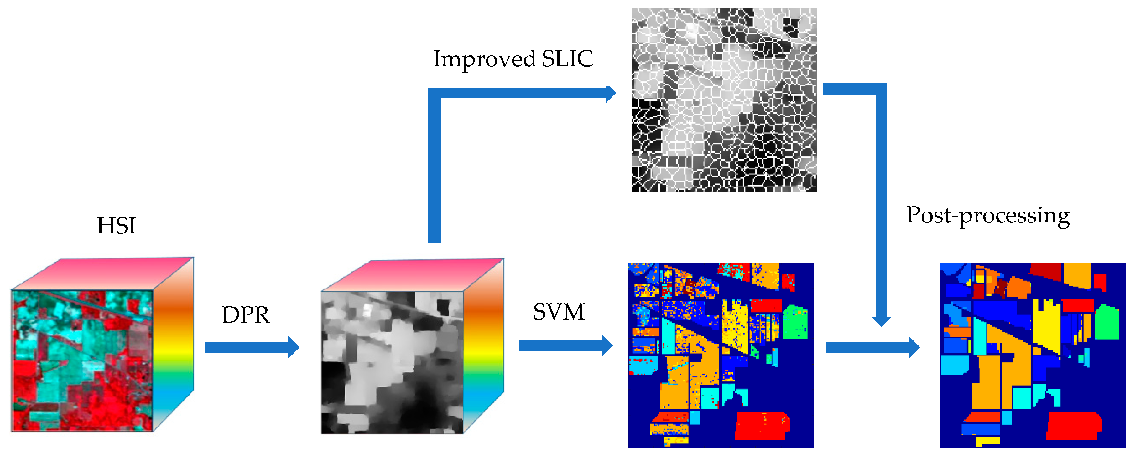
To better understand the proposed classification scheme, the overall workflow of the integration of DPR, SVM and superpixel segmentation is elaborated in Figure 2. In this scheme, the DPR technique is responsible for denoising, while retaining the class boundary information better. The SVM method has good classification performance for high-dimensional data with small labeled samples. Similar to the other two-step classification methods, the use of a superpixel in post-processing can significantly improve the classification accuracy. The proposed approach effectively integrates their strengths, and the experimental results also confirm the effectiveness of the proposal.
3. Experimental Results and Analysis
3.1. Datasets
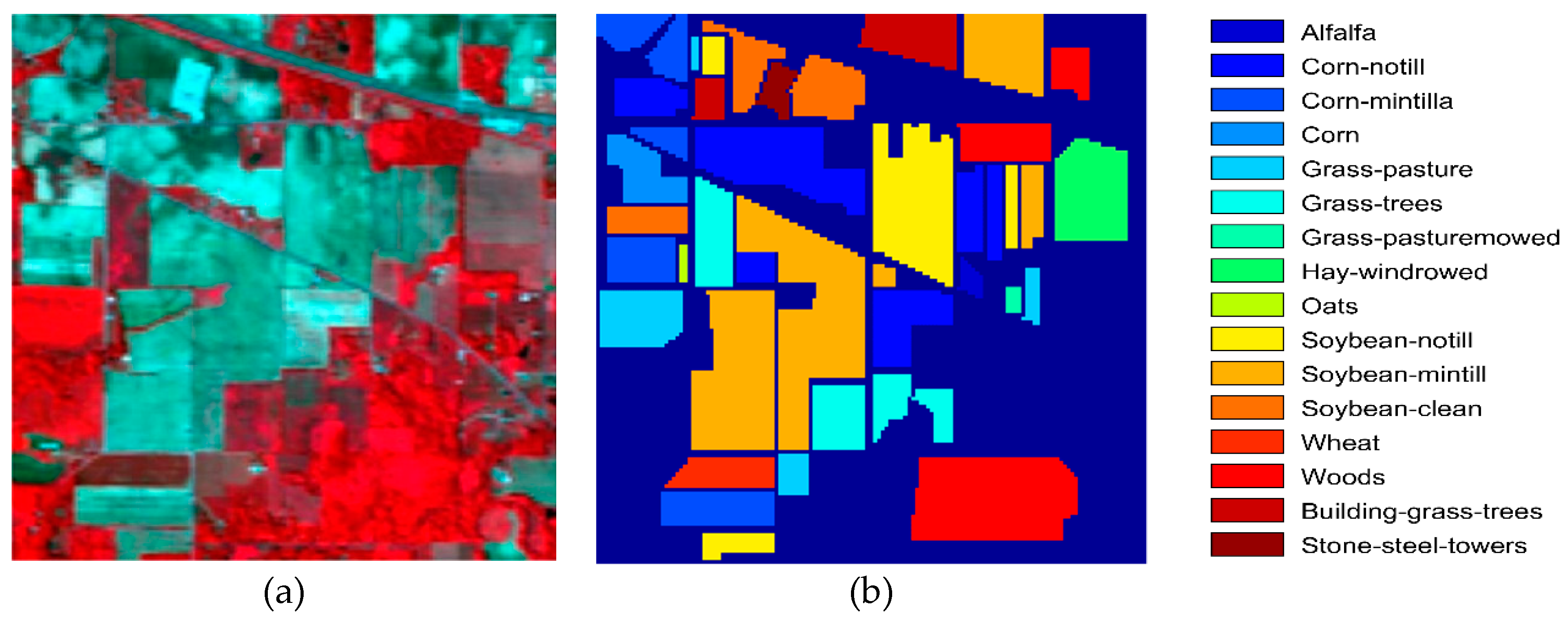
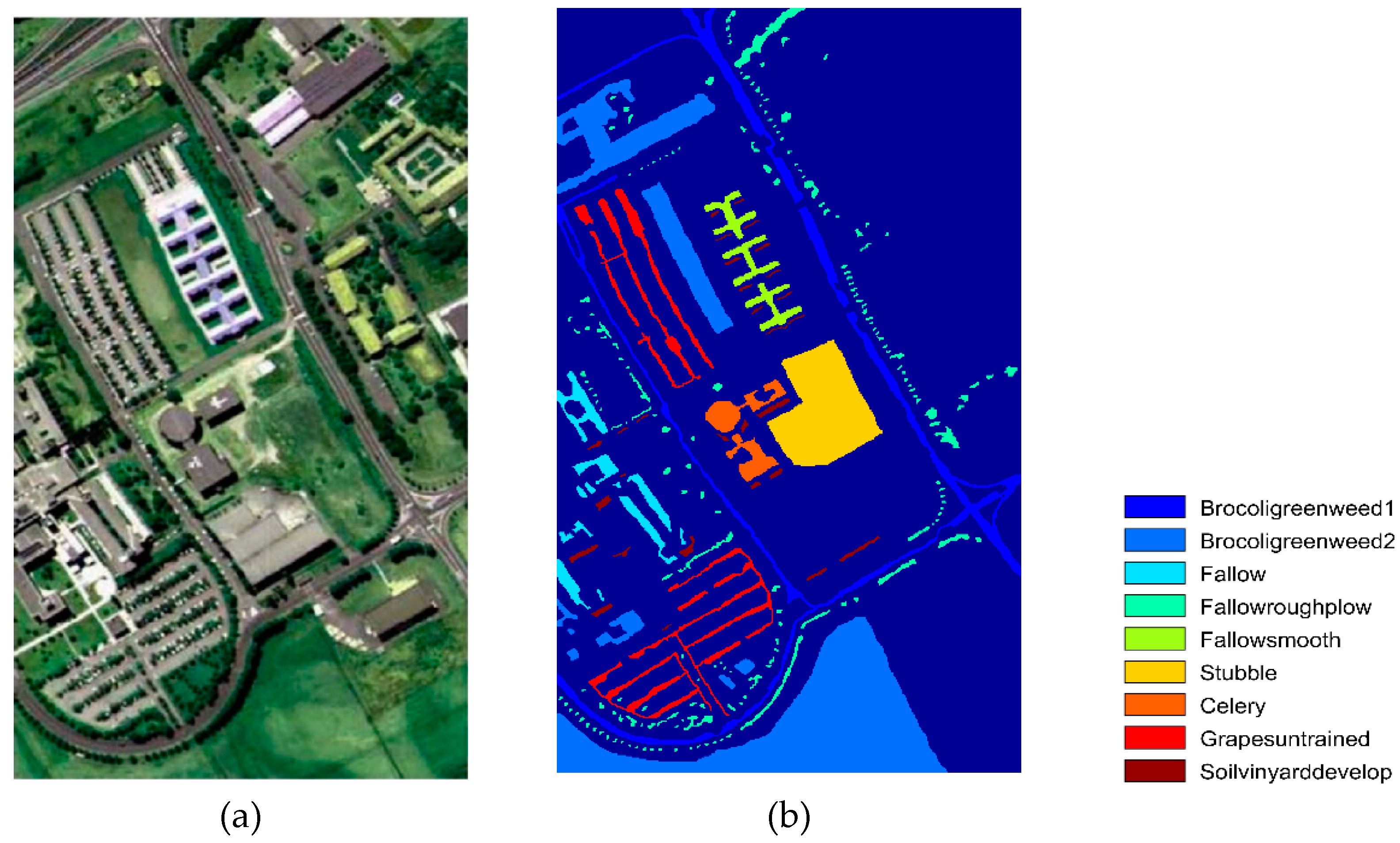
The effectiveness of the proposed DPR-SVM-SP method is tested on three public real hyperspectral datasets, i.e., Indian Pines dataset, Pavia University dataset and Salinas dataset. The reasons why these three datasets are widely used to test the performance of HSI classification algorithms are: (1) The Indian Pines dataset is a severely unbalanced dataset with 16 classes. The maximum class and the minimum class contain 2455 pixels and only 20 pixels, respectively. (2) Although there are only nine classes in Pavia University dataset, objects of different classes, even objects in the same class, show great differences in spatial structure. (3) In the Salinas dataset, there are two spatial adjacent classes that have a little difference in spectral features. All of these factors pose a challenge to the HSI classification methods. These three hyperspectral datasets are available online at http://www.ehu.eus/ccwintco/index.php/Hyperspectral_Remote_Sensing_Scenes.
3.2. Experimental Design
In the experiments, 5% of pixels from each class for the Indian Pines dataset and 1% of pixels per class for the Pavia University and Salinas dataset are randomly labeled as training sets, respectively. The rest make up the test set. To overcome the deviation caused by random sampling on classification results, the classification accuracy provided in this study is the statistical results of ten independent trials with randomly selected training sets, i.e., the mean and standard deviation of ten classification results. The classification results are evaluated by three popular indices, overall accuracy (OA), average accuracy (AA), and kappa coefficient (κ).
3.3. Classification Result
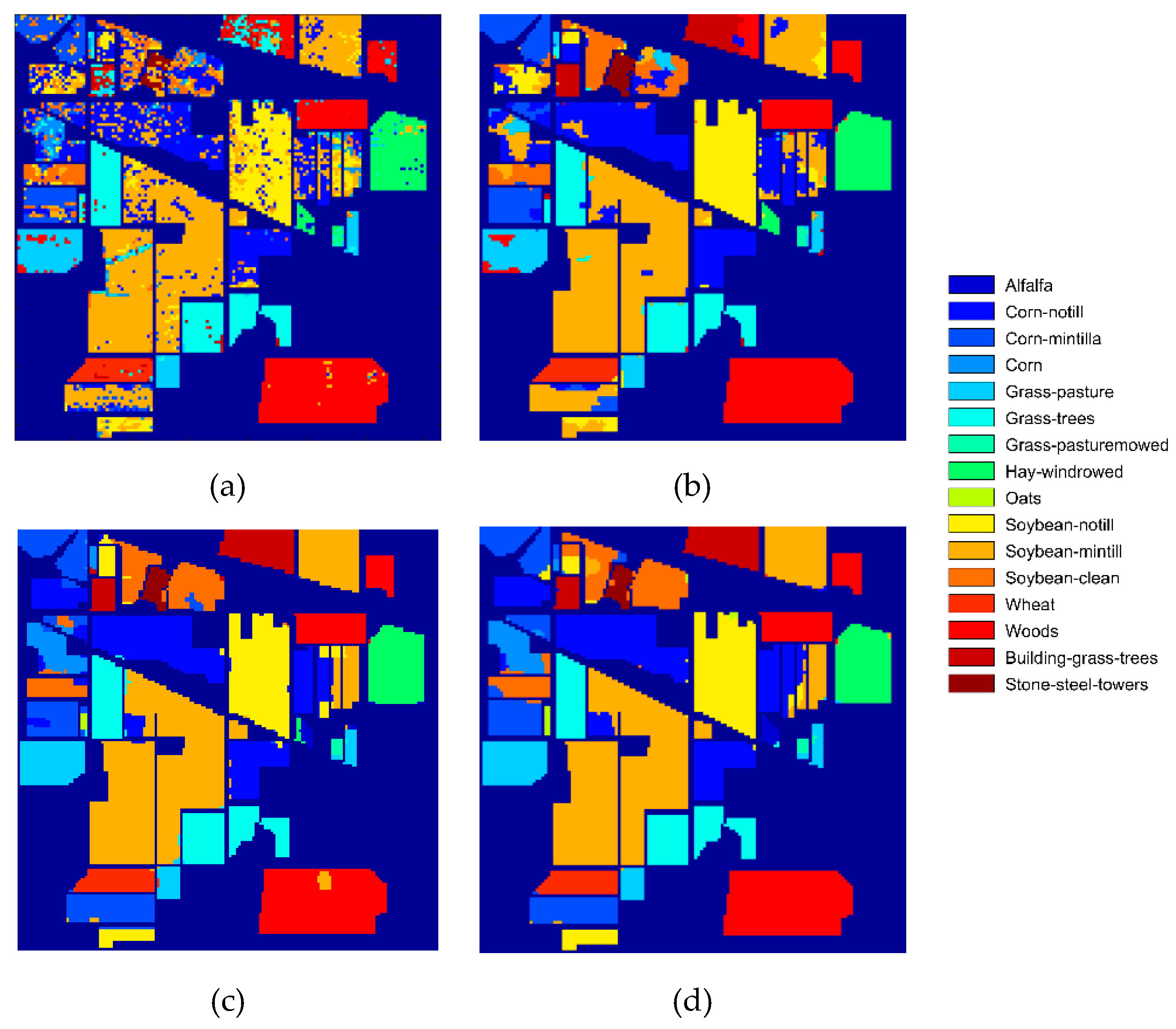
Table 2 reports the statistical results of ten independent classifications provided by SVM only, SVM and superpixel obtained by improved SLIC algorithm (SVM-SP), DPR+SVM+superpixel obtained by PCA+original SLIC algorithm (DPR-SVM-POS), and the proposed scheme DPR-SVM-SP on the Indian Pines dataset. The SVM-SP method means that the classification is done pixel-wise by using SVM, and then the superpixel is used to improve the classification result in post-processing. The classification results obtained by SVM using only spectral information are unsatisfied on this hyperspectral dataset. The use of a superpixel in the SVM-SP approach has led to a significant improvement in the classification results, that is, the classification accuracy is increased by about 10%. According to the classification accuracy, it seems that all samples in class Alfalfa (46 samples) and class Oats (20 samples) are misclassified, except the labeled sample itself. This is probably because the volumes of the two categories are so small, and their spectral features are so similar to those of their spatial neighbor classes that they are divided into other classes in superpixel segmentation. Satisfactory results have been acquired by the proposed classification scheme, and the classification accuracies of almost all classes are more than 90%, except for Corn. The proposal shows a good classification performance on the three minimum classes. It indicates that using DPR and superpixel together in HSI classification is good for discriminating land covers of interest, as shown in Figure 6.
In Table 3, compared with the result provided by SVM on the Pavia University dataset, the classification accuracy (OA) obtained by SVM-SP and DPR-SVM-SP is improved by about 6% and 10%, respectively. Statistical results on class Soil-vineyard-develop explain that the spectral characteristics of its pixels are very similar to each other. The use of superpixels in post-processing has a slight effect on its classification result. This shows that the improved SLIC algorithm can still better segment the class in which the spatial distribution of pixels is very scattered, as shown by the light green class “Fallowroughplow” in Figure 4b. However, the breakdown boundary and the very small fragments resulted in a decline in classification accuracy of this class, due to the application of the DPR technique. Maybe the DPR method does not deal with this case very well. The visual classification results of the Pavia University dataset are shown in Figure 7.
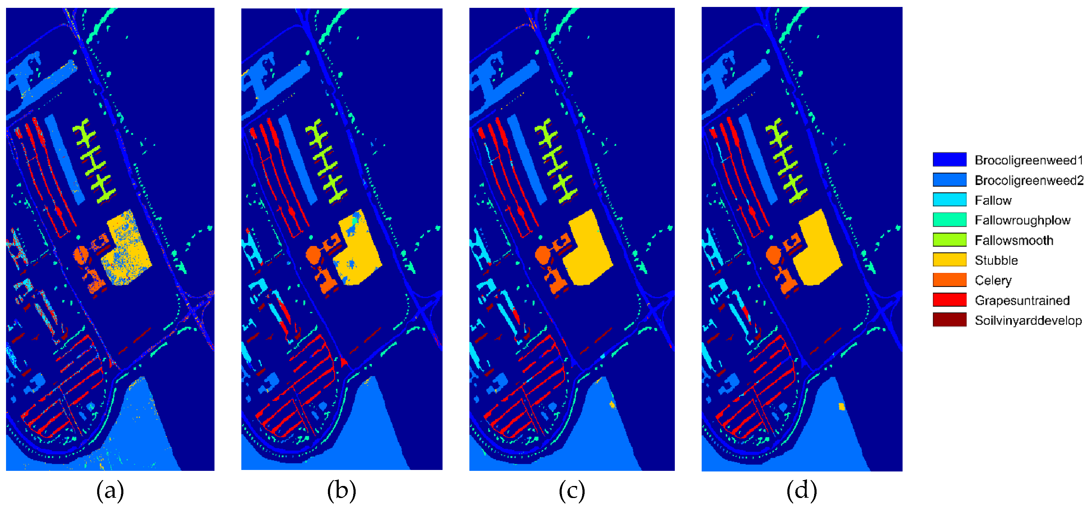
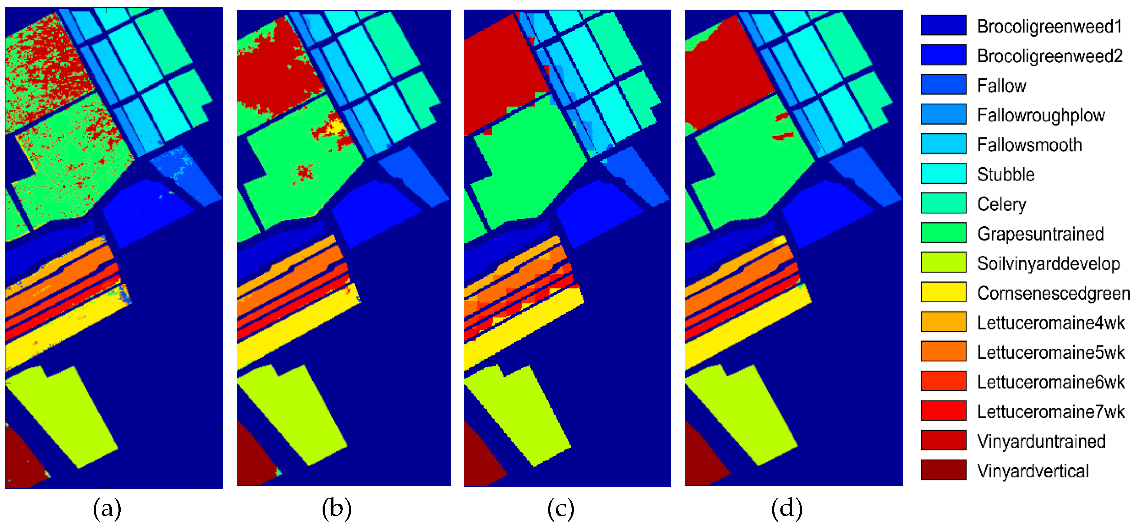
Table 4 lists an accurate classification result achieved by the proposed method for the Salinas dataset. For this hyperspectral dataset, the correct classification between class “Grapes-untrained” and class “Grapes-untrained” is a challenging problem for existing methods, because these two categories are actually the same [60]. That is to say that their spectral features are highly similar. We can easily know from Figure 8a that most of misclassified pixels belong to these two classes. As can be seen from Table 4 and Figure 8d, the proposed method is a good solution to the problem. In addition, we have also observed that the standard deviation of classification accuracy is very small, even for each category. It means that there is good stability of the proposed classification scheme.
As can be seen form Table 2, Table 3 and Table 4, compared with the SVM-SP method, the proposed method improves significantly the classification accuracy because of the use of DPR. Compared to DPR-SVM-POS approach, the proposed scheme still has good classification performance. This comparison also confirms the effectiveness of the improved SLIC. It should be noted that the improved SLIC algorithm can directly segment HSI into superpixels without using PCA in advance, and is free of parameters.
3.4. Comparative Test
To compare the proposed classification scheme with other state-of-the-art methods, it is important to select the same dataset, the same number of labeled samples and those classification approaches related to superpixels or spatial structure. Based on this consideration, we compare the proposal with different HSI classification methods, including SVM with the Extended Morphological Profile (EMP) and superpixels (EMP-SP-SVM) [56], multi-scale superpixel (MSP) and subspace-based SVM (MSP-SVMsub) [57], superpixel-based discriminative sparse model (SBDSM) [52], superpixel and extreme learning machines (SP-ELM) [55], superpixel-based spatial pyramid representation (SP-SPR) [61], multiple kernel learning-based low rank representation at superpixel level (SP-MKL-LRR) [48] segmented stacked autoencoder (S-SAE) [18] and spectral–spatial correlation segmentation-based classifier (SoCRATE) [21], SuperPCA [54]. All of these approaches try to use superpixels or spatial structure to improve the accuracy of classification results. Table 5 reports the comparison results of nine methods on the same three hyperspectral datasets. The classification accuracy of these nine methods comes from their papers.
There is no significant difference between the different classification methods because of the higher classification accuracy. For example, there is only a slight difference between our proposal and SP-SPR, SBDSM, S-SAE, and SP-ELM methods on the corresponding datasets. However, our method outperforms MSP-SVMsub (87.62% vs. 84.01%) and EMP-SP-SVM (93.74% vs. 91.64%) on the Indian Pines dataset with small training samples. What needs to be explained is that, on the Pavia University dataset, the classification accuracy (93.97%) of SP-MKL-LRR with labeled ratio 15% is still lower than our result (97.7%) with a labeled ratio of 1%. It indicates that our method makes better use of spatial information in the classification process. In case of the segmentation-aided sampling, SoCRATE is superior to our method (98.18% vs. 96%) on the Indian Pines dataset, but classification results (97.7% vs. 93.44%) on the Pavia University dataset and that (99.16% vs. 98.64%) on the Salinas dataset indicate that the proposed scheme is better than SoCRATE. Although the proposal is slightly superior to the SuperPCA method on the Indian Pines and Pavia University datasets, the classification result (98.97% vs. 98.12%) on the Salinas dataset is better than ours. When the SuperPCA method and multi-scale superpixel were combined, the MSuperPCA method presented a good classification result [54]. The results of Table 5 show that the classification accuracy can be significantly improved by using the spatial information and the improved SLIC algorithm effectively.
4. Parameter Analysis
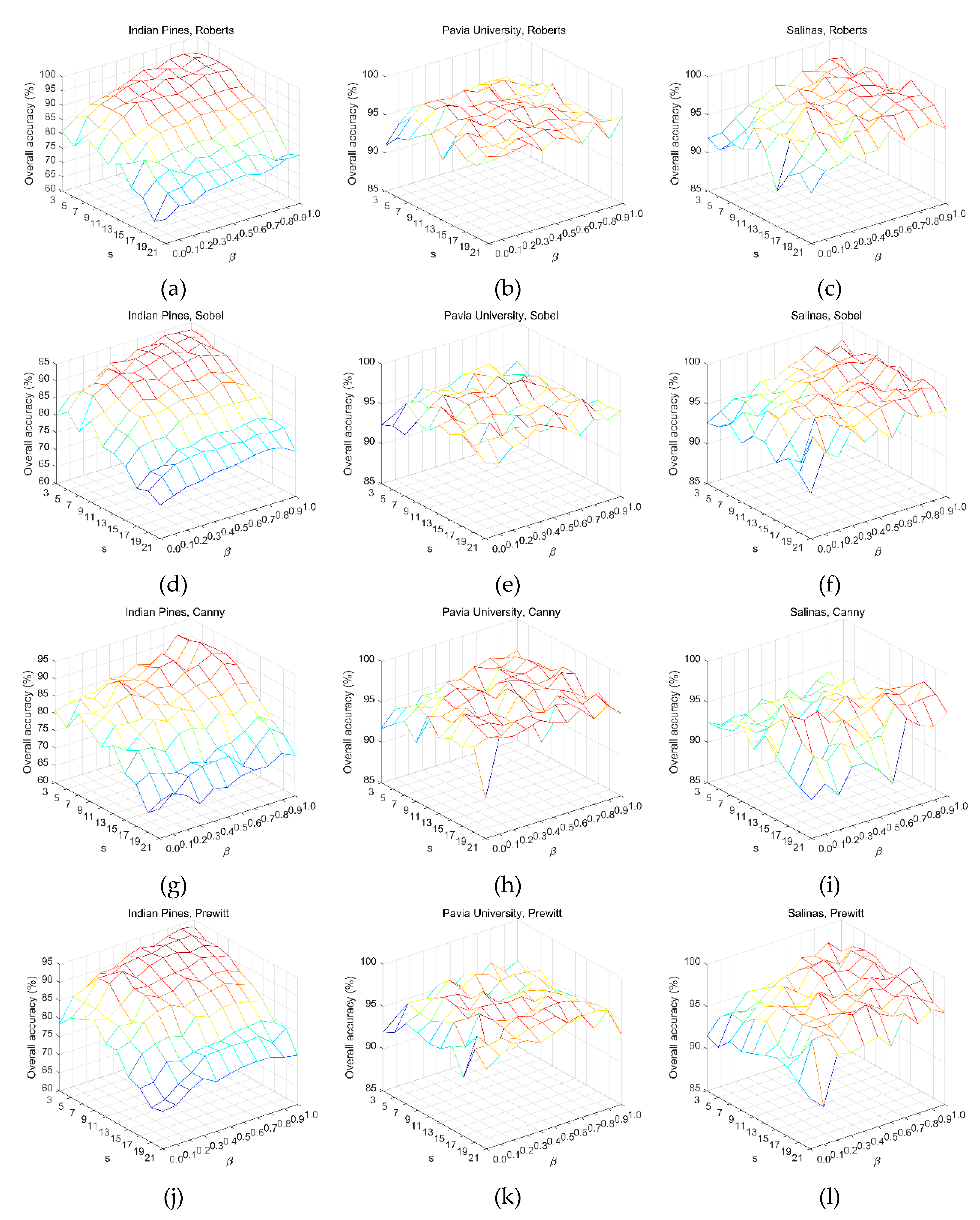
In this section, we discuss the effects of the parameters adopted in the proposed scheme on classification results on the three hyperspectral datasets. Parameter β controls the contribution of discontinuity calculated by edge detection operator to the smooth image in the DPR method. Segmentation scale s dominates the size of superpixels in SLIC algorithm. Furthermore, the effects of different edge detection operators on the classification results are also analyzed.
Figure 9 shows the classification results on three hyperspectral datasets for four different edge detection operators. For Indian Pines dataset, with the increase of superpixel volume, the classification accuracy of the four operators shows an obvious downward trend. This may be due to the fact that the number of object classes contained in large superpixels exceeds the number of clusters, thus undermining the homogeneity of superpixels. All the four operators show better classification performance on Pavia University dataset, and almost all classification accuracies are more than 90%, especially Robert operator and Sobel operator. The reason should be that Pavia University dataset has only nine classes and that they have significant spatial separation. The satisfactory classification results can be obtained on Salinas dataset by using Robert, Sobel and Prewitt operators, most of which are above 95%. The best results achieved by these four operators on different datasets are recorded in Table 6.
It is easy to see from table 6 that Robert operator provides two of the three best classification accuracy. In particular, compared with the other three operators, Robert operator has an obvious advantage on Indian Pines dataset. Almost perfect classification result is obtained by using Robert operator on Salinas dataset. Canny operator outperforms the other three operators on Pavia University dataset. This is because the Canny operator is a second-order differential operator and has a good ability to recognize irregular boundaries. Unlike Indian Pines and Salinas datasets, the difference of classification accuracy among the four operators on Pavia University dataset is less than 0.3%. In other words, it is acceptable to adopt Robert operator in the proposed method.
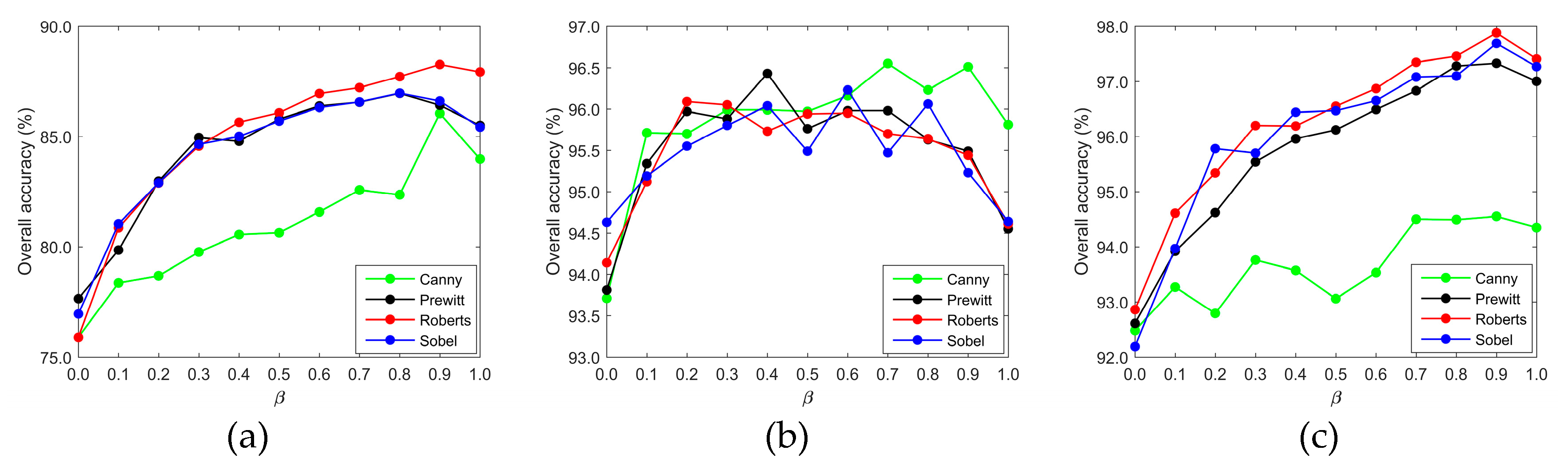
Figure 10 exhibits the variation of the average classification accuracy with the increase of β. Each point in Figure 10 is the average of the classification results obtained by the proposed scheme on ten different superpixel segmentation scales s and with the same β. Furthermore, the classification accuracy for the fixed segmentation scale s is the average of the classification results of the training set generated randomly for ten times. It is known from Equation (5) that β = 0 means to classify HSI on the original dataset without data smoothing; β = 1 represents to denoise HSI completely using the boundary information contained in the neighbors of the tested pixel, while neglecting the spectral band information of the tested pixel itself.
For two AVIRIS datasets, the Indian Pines and Salinas, the average classification accuracy becomes better and better as β value increase. This indicates that all the other three operators, except canny operators, can detect effectively class boundary, and this information plays a dominant role in the DPR method. The reason may be that, as shown in Figure 3b and Figure 5b, the boundary of each category in these two datasets is essentially regular, but the acquirement of the best β value (0.8 or 0.9) depends on the operator used in the DPR strategy. Although the classification results obtained by using the three operators are not much different, the Robert operator still has some advantage.
The variation of average classification accuracy does not show obvious regularity on the Pavia University dataset. The great increasing of the average classification accuracy with the increase of β value from 0 to 0.1 or 0.2 explains that it is necessary to adopt edge detection operators in DPR method. While β value varies from 0.7 to 1, the classification accuracy obtained by Canny operator is still superior, because of its good ability to extract an irregular class boundary. On this dataset, the acquirement of the best β is seriously depended on the operator applied in DPR strategy.
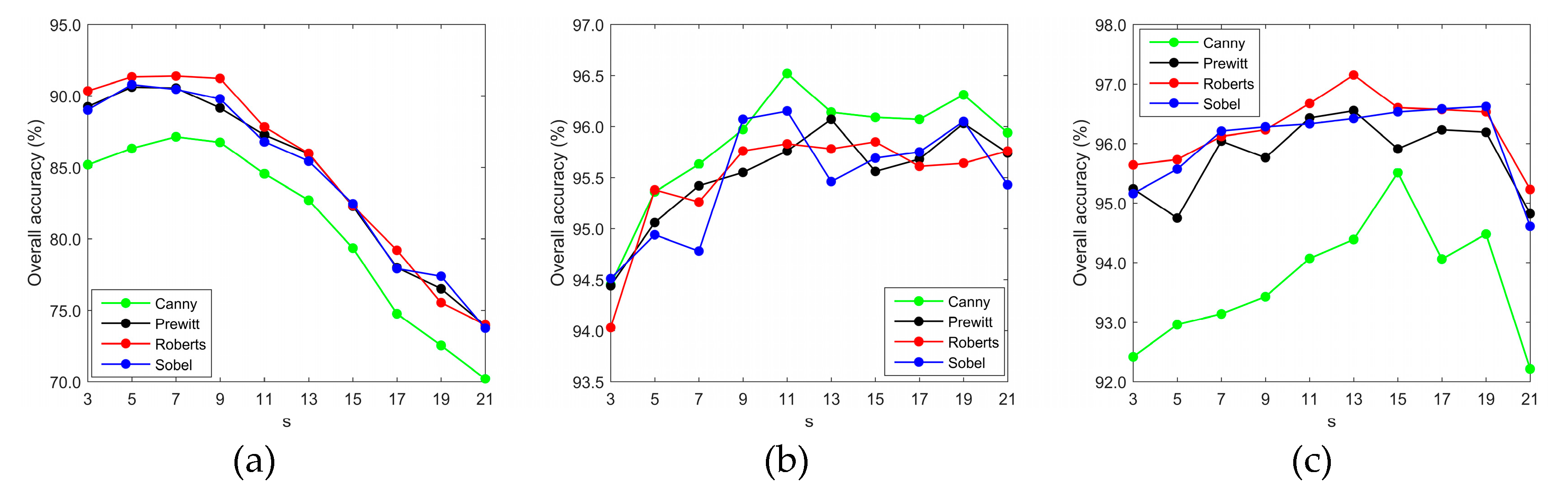
Each datum in Figure 11 is the average of the classification results obtained by the proposal for 11 different β values and with the same segmentation scale s. For the Indian pines dataset, the average classification accuracy shows a significant downward trend as the segmentation scale s changes from 9 to 21. Since the Indian Pines dataset with size 145 × 145 has 16 classes, large-scale segmentation will inevitably reduce the homogeneity of superpixels. In post-processing, the heterogeneity of superpixels obviously leads to a distinctive decrease in classification accuracy. Contrary to the case of the Indian Pines dataset, satisfactory classification results have been obtained on the Pavia University dataset when s was from 9 to 21. One can see from Figure 8b that all the average classification accuracies are over 95.5%. As shown in Figure 4b, a great difference in spatial structure of the objects in the same class implies that using large scales in the SLIC algorithm will achieve a better segmentation effect on this dataset. In superpixel addition, the advantage of the Canny operator in detecting an irregular boundary is proved again. On the Salinas dataset, the Sobel operator shows good stability with the increase of the volume of. There is no significant difference in average classification accuracy among Sobel operator, Robert operator and Prewitt operator when the segmentation scale s varies from 7 to 19. The reason behind this lies in that in this hyperspectral dataset, the regular class shape and the absence of the class with a very small volume make the proposed method insensitive to the segmentation scale.
Table 7 shows how the average classification accuracy on three datasets varies with the increasing of the number of training samples. The visualization of result in Table 7 is displayed in Figure 12. As seen from Table 7 and Figure 12, the classification accuracy has been greatly improved by using spatial information in pre-processing or post-processing. For the Pavia University dataset, the classification accuracy of SVM-SP and DPR-SVM-SP increases slightly as the number of training samples is changed from 2 to 10%. This is because the classification accuracy is so high that there is no room for improvement. The classification accuracy of DPR-SVM-SP on AVIRIS dataset Salinas is more than 95% when the labeled ratio is great than or equal to 0.3%. It indicates that the proposed method can achieve the satisfactory classification result with small training samples. The classification results on the Indian Pines dataset have not shown the growth we expect, when the labeled ratio is greater than 6%. Maybe, most of the pixels that are correctly newly classified are in the superpixels that have already been correctly classified previously.
5. Conclusions
In this study, a technique for measuring the similarity of two pixels in HSI is proposed to address the problem of dividing HSI into superpixels directly by using the SLIC algorithm without using a PCA method. The adoption of this new similarity in the SLIC algorithm will also make it a non-parametric algorithm and easy to use. The experimental results of this work confirm the success of this attempt. Based on the improved SLIC algorithm, SVM and DPR methods, an effective classification scheme for hyperspectral data is developed. The classification accuracy can be significantly improved by utilizing DPR method in preprocessing and superpixel in post-processing. Experimental results on three real hyperspectral datasets widely used to test the performance of HSI classification approaches demonstrate the effectiveness of the proposed method.
In the proposed classification scheme, the DPR strategy, SVM and superpixels obtained by the improved SLIC can be replaced with other denoising techniques, classification algorithms or superpixels detected by other methods. That is to say that among the many combinations, only one of them has been considered in this paper. To an extent, the proposal is a general semi-supervised classification scheme. The DPR method with Robert operator has a good denoising effect on the hyperspectral data with relatively regular class boundary. However, for the HSI in which some classes are composed of many very small fragments, DPR with Canny operator seems to have a good de-noising performance. In summary, one can see from Table 6 and Table 7 that the proposal can achieve good classification results.
Author Contributions
C.L. and F.X. conceived and designed the experiments; C.L. performed the experiments; J.Y. and C.J. analyzed the data and developed the graphs and tables; F.X. and C.J. wrote the paper.
Funding
This research was funded by the National Natural Science Foundation of China, grants number 41801340 and 41771178; and Natural Science Foundation of Liaoning Province, grant number 20180550238.
Acknowledgments
We would like to sincerely thank anonymous reviewers for their very valuable suggestions and professional comments to improve the manuscript. We would also like to express our sincere gratitude to Editor Xia for her kind help.
Conflicts of Interest
The authors declare no conflict of interest.
References
- Kanning, M.; Siegmann, B.; Jarmer, T. Regionalization of uncovered agricultural soils based on organic carbon and soil texture estimations. Remote Sens. 2016, 8, 927. [Google Scholar] [CrossRef]
- Heldens, W.; Heiden, U.; Esch, T.; Stein, E.; Müller, A. Can the future Enmap mission contribute to urban applications? A literature survey. Remote Sens. 2011, 3, 1817–1846. [Google Scholar] [CrossRef]
- Clark, M.L.; Roberts, D.A. Species-level differences in hyperspectral metrics among tropical rainforest trees as determined by a tree-based classifier. Remote Sens. 2012, 4, 1820–1855. [Google Scholar] [CrossRef]
- Zhang, L.; Tao, D.; Xin, H. Sparse transfer manifold embedding for hyperspectral target detection. IEEE Trans. Geosci. Remote Sens. 2013, 52, 1030–1043. [Google Scholar] [CrossRef]
- Du, B.; Zhang, L. Random-selection-based anomaly detector for hyperspectral imagery. IEEE Trans. Geosci. Remote Sens. 2011, 49, 1578–1589. [Google Scholar] [CrossRef]
- Melgani, F.; Bruzzone, L. Classification of hyperspectral remote sensing images with support vector machines. IEEE Trans. Geosci. Remote Sens. 2004, 42, 1778–1790. [Google Scholar] [CrossRef] [Green Version]
- Chi, M.; Bruzzone, L. Semisupervised classification of hyperspectral images by svms optimized in the primal. IEEE Trans. Geosci. Remote Sens. 2007, 45, 1870–1880. [Google Scholar] [CrossRef]
- Bazi, Y.; Melgani, F. Toward an optimal svm classification system for hyperspectral remote sensing images. IEEE Trans. Geosci. Remote Sens. 2006, 44, 3374–3385. [Google Scholar] [CrossRef]
- Tuia, D.; Volpi, M.; Mura, M.D.; Rakotomamonjy, A.; Flamary, R. Automatic feature learning for spatio-spectral image classification with sparse svm. IEEE Trans. Geosci. Remote Sens. 2014, 52, 6062–6074. [Google Scholar] [CrossRef]
- Böhning, D. Multinomial logistic regression algorithm. Ann. Inst. Statist. Math. 1992, 44, 197–200. [Google Scholar] [CrossRef]
- Li, J.; Bioucas-Dias, J.M.; Plaza, A. Semi-supervised hyperspectral image segmentation using multinomial logistic regression with active learning. IEEE Trans. Geosci. Remote Sens. 2010, 48, 4085–4098. [Google Scholar]
- Feng, J.; Jiao, L.; Liu, F.; Sun, T.; Zhang, X. Unsupervised feature selection based on maximum information and minimum redundancy for hyperspectral images. Patt. Recog. 2016, 51, 295–309. [Google Scholar] [CrossRef]
- Xie, F.; Li, F.; Lei, C.; Yang, J.; Zhang, Y. Unsupervised band selection based on artificial bee colony algorithm for hyperspectral image classification. Applied Soft Computing. 2019, 75, 428–440. [Google Scholar] [CrossRef]
- Chen, Y.; Nasrabadi, N.M.; Tran, T.D. Hyperspectral image classification using dictionary-based sparse representation. IEEE Trans. Geosci. Remote Sens. 2011, 49, 3973–3985. [Google Scholar] [CrossRef]
- Ni, D.; Ma, H. Hyperspectral image classification via sparse code histogram. IEEE Geosci. Remote Sens. Lett. 2015, 12, 1843–1847. [Google Scholar]
- Tan, K.; Hu, J.; Li, J.; Du, P. A novel semi-supervised hyperspectral image classification approach based on spatial neighborhood information and classifier combination. ISPRS J. Photo. 2015, 105, 19–29. [Google Scholar] [CrossRef]
- Ghamisi, P.; Mura, M.D.; Benediktsson, J.A. A survey on spectral–spatial classification techniques based on attribute profiles. IEEE Trans. Geos. Remote Sens. 2015, 53, 2335–2353. [Google Scholar] [CrossRef]
- Paul, S.; Kumar, D.N. Spectral–spatial classification of hyperspectral data with mutual information based segmented stacked auto-encoder approach. ISPRS J. Photo. Remot. Sens. 2018, 138, 265–280. [Google Scholar] [CrossRef]
- Ghamisi, P.; Benediktsson, J.A.; Ulfarsson, M.O. Spectral–spatial classification of hyperspectral images based on hidden Markov random fields. IEEE Trans. Geos. Remote Sens. 2014, 52, 2565–2574. [Google Scholar] [CrossRef]
- Pan, B.; Shi, Z.; Xu, X. Mugnet: Deep learning for hyperspectral image classification using limited samples. ISPRS J. Photogram. Rem. Sens. 2018, 145, 108–119. [Google Scholar] [CrossRef]
- Appice, A.; Malerba, D. Segmentation-aided classification of hyperspectral data using spatial dependency of spectral bands. ISPRS J. Photogram. Rem. Sens. 2019, 147, 215–231. [Google Scholar] [CrossRef]
- Jia, S.; Zhang, X.; Li, Q. Spectral–spatial hyperspectral image classification using regularized low-rank representation and sparse representation-based graph cuts. IEEE J. Sel. Top. Appl. Earth Obs. 2017, 8, 2473–2484. [Google Scholar] [CrossRef]
- Yu, H.; Gao, L.; Li, J.; Li, S.; Zhang, B.; Benediktsson, J. Spectral–spatial hyperspectral image classification using subspace-based support vector machines and adaptive Markov random fields. Remote Sens. 2016, 8, 355. [Google Scholar] [CrossRef]
- Li, H.; Zheng, H.; Han, C.; Wang, H.; Miao, M. Onboard spectral and spatial cloud detection for hyperspectral remote sensing images. Remote Sens. 2018, 10, 152. [Google Scholar] [CrossRef]
- Shuai, L.; Licheng, J.; Shuyuan, Y. Hierarchical sparse learning with spectral–spatial information for hyperspectral imagery denoising. Sensors 2016, 16, 1718. [Google Scholar] [CrossRef]
- Li, W.; Prasad, S.; Fowler, J.E. Hyperspectral image classification using gaussian mixture models and markov random fields. IEEE Geosci. Remote Sens. Lett. 2013, 11, 153–157. [Google Scholar] [CrossRef]
- Li, J.; Bioucas-Dias, J.M.; Plaza, A. Spectral–spatial hyperspectral image segmentation using subspace multinomial logistic regression and Markov random fields. IEEE Trans. Geosci. Remote Sens. 2012, 50, 809–823. [Google Scholar] [CrossRef]
- Li, J.; Khodadadzadeh, M.; Plaza, A.; Jia, X.; Bioucas-Dias, J.M. A discontinuity preserving relaxation scheme for spectral–spatial hyperspectral image classification. IEEE J. Sel. Top. Appl. Earth Obs. 2017, 9, 625–639. [Google Scholar] [CrossRef]
- He, L.; Li, J.; Plaza, A.; Li, Y. Discriminative Low-Rank Gabor Filtering for Spectral–Spatial Hyperspectral Image Classification. IEEE Trans. Geosci. Remote Sens. 2017, 55, 1381–1395. [Google Scholar] [CrossRef]
- Li, A.; Qin, A.; Shang, Z.; Tang, Y.Y. Spectral–spatial Sparse Subspace Clustering Based on Three-Dimensional Edge-Preserving Filtering for Hyperspectral Image. Int. J. Pattern Recognit. Artif. Intell. 2018. [Google Scholar] [CrossRef]
- Charles, A.S.; Rozell, C.J. Spectral Super resolution of Hyperspectral Imagery Using Reweighted l1 Spatial Filtering. IEEE Geosci. Remote Sens. Lett. 2014, 11, 602–606. [Google Scholar] [CrossRef]
- Chen, C.; Zhou, L.; Guo, J.; Li, W.; Su, H.; Guo, F. Gabor-Filtering-Based Completed Local Binary Patterns for Land-Use Scene Classification. In Proceedings of the IEEE International Conference on Multimedia Big Data, Beijing, China, 20–22 April 2015. [Google Scholar]
- Kang, X.; Li, S.; Benediktsson, J.A. Spectral–spatial hyperspectral image classification with edge-preserving filtering. IEEE Trans. Geosci. Remote Sens. 2014, 52, 2666–2677. [Google Scholar] [CrossRef]
- Jia, S.; Shen, L.; Li, Q. Gabor feature-based collaborative representation for hyperspectral imagery classification. IEEE Trans. Geosci. Remote Sens. 2015, 53, 1118–1129. [Google Scholar]
- Benediktsson, J.A.; Palmason, J.A.; Sveinsson, J.R. Classification of hyperspectral data from urban areas based on extended morphological profiles. IEEE Trans. Geosci. Remote Sens. 2005, 43, 480–491. [Google Scholar] [CrossRef]
- Felzenszwalb, P.F.; Huttenlocher, D.P. Efficient graph-based image segmentation. Int. J. Comput. Vis. 2004, 59, 167–181. [Google Scholar] [CrossRef]
- Shi, J.; Malik, J. Normalized cuts and image segmentation. IEEE Trans. Pattern Anal. Mach. Intell. 2000, 22, 888–905. [Google Scholar] [Green Version]
- Lu, T.; Wang, J.; Zhou, H.; Jiang, J.; Ma, J.; Wang, Z. Rectangular-Normalized Superpixel Entropy Index for Image Quality Assessment. Entropy 2018, 20, 947. [Google Scholar] [CrossRef]
- Comaniciu, D.; Meer, P. Mean shift: A robust approach toward feature space analysis. IEEE Trans. Pattern Anal. Mach. Intell. 2002, 24, 603–619. [Google Scholar] [CrossRef]
- Levinshtein, A.; Stere, A.; Kutulakos, K.N.; Fleet, D.J.; Dickinson, S.J.; Siddiqi, K. Turbopixels: Fast superpixels using geometric flows. IEEE Trans. Patt. Anal. Mach. Intell. 2009, 31, 2290–2297. [Google Scholar] [CrossRef]
- Achanta, R.; Shaji, A.; Smith, K.; Lucchi, A.; Fua, P.; Sabine, S. SLIC superpixels compared to state-of- the-art superpixel methods. IEEE Trans. Patt. Analy. Mach. Intell. 2012, 34, 2274–2282. [Google Scholar] [CrossRef]
- Li, J.; Zhang, H.; Zhang, L. Efficient superpixel-level multitask joint sparse representation for hyperspectral image classification. IEEE Trans. Geosci. Remote Sens. 2015, 53, 5338–5351. [Google Scholar]
- Fang, L.; Li, S.; Duan, W.; Ren, J.; Benediktsson, J.A. Classification of hyperspectral images by exploiting spectral–spatial information of superpixel via multiple kernels. IEEE Trans. Geosci. Remote Sens. 2015, 53, 6663–6674. [Google Scholar] [CrossRef]
- Saranathan, A.M.; Parente, M. Uniformity-based superpixel segmentation of hyperspectral images. IEEE Trans. Geosci. Remote Sens. 2016, 54, 1419–1430. [Google Scholar] [CrossRef]
- Tan, N.; Xu, Y.; Goh, W.B.; Liu, J. Robust multi-scale superpixel classification for optic cup localization. Comput. Med. Imag. Grap. 2015, 40, 182–193. [Google Scholar] [CrossRef]
- Wang, Q.; Lin, J.; Yuan, Y. Salient band selection for hyperspectral image classification via manifold ranking. IEEE Trans. Neural Netw. 2016, 27, 1279–1289. [Google Scholar] [CrossRef]
- Wang, Y.; Zhang, Y.; Song, H. A spectral-texture kernel-based classification method for hyperspectral images. Remote Sens. 2016, 8, 919. [Google Scholar] [CrossRef]
- Zhan, T.; Sun, L.; Xu, Y.; Yang, G.; Zhang, Y.; Wu, Z. Hyperspectral classification via superpixel kernel learning-based low rank representation. Remote Sens. 2018, 10, 1639. [Google Scholar] [CrossRef]
- Fan, J.; Chen, T.; Lu, S. Superpixel guided deep-sparse-representation learning for hyperspectral image classification. IEEE Trans. Circuits Syst. Video Technol. 2018, 28, 3163–3173. [Google Scholar] [CrossRef]
- Jia, S.; Deng, B.; Zhu, J.; Jia, X.; Li, Q. Superpixel-based multitask learning framework for hyperspectral image classification. IEEE Trans. Geosci. Remote Sens. 2017, 99, 2575–2588. [Google Scholar] [CrossRef]
- Jia, S.; Deng, B.; Huang, Q. An efficient superpixel-based sparse representation framework for hyperspectral image classification. Int. J. Wavelets Multiresolution Inf. Process. 2017, 15. [Google Scholar] [CrossRef]
- Fang, L.; Li, S.; Kang, X.; Benediktsson, J.A. Spectral–spatial classification of hyperspectral images with a superpixel-based discriminative sparse model. IEEE Trans. Geosci. Remote Sens. 2015, 53, 4186–4201. [Google Scholar] [CrossRef]
- Zhang, S.; Li, S.; Fu, W.; Fang, L. Multi-scale superpixel-based sparse representation for hyperspectral image classification. Remote Sens. 2017, 9, 139. [Google Scholar] [CrossRef]
- Jiang, J.; Ma, J.; Chen, C.; Wang, Z.; Cai, Z.; Wang, L. SuperPCA: A Superpixel wise PCA Approach for Unsupervised Feature Extraction of Hyperspectral Imagery. IEEE Trans. Geosci. Remote Sens. 2018, 56, 4581–4593. [Google Scholar] [CrossRef]
- Duan, W.; Li, S.; Fang, L. Spectral–spatial hyperspectral image classification using superpixel and extreme learning machines. Patt. Recog. 2014, 483, 159–167. [Google Scholar]
- Liu, T.; Gu, Y.; Chanussot, J.; Mura, M.D. Multimorphological superpixel model for hyperspectral image classification. IEEE Trans. Geosci. Remote Sens. 2017, 55, 6950–6963. [Google Scholar] [CrossRef]
- Yu, H.; Gao, L.; Liao, W.; Zhang, B.; Pižurica, A.; Philips, W. Multiscale superpixel-level subspace-based support vector machines for hyperspectral image classification. IEEE Geosci. Remote Sens. Lett. 2017, 14, 2142–2146. [Google Scholar] [CrossRef]
- Cao, J.; Zhao, C.; Wang, B. Deep convolutional networks with superpixel segmentation for hyperspectral image classification. In Proceedings of the IEEE International Geoscience and Remote Sensing Symposium, Beijing, China, 10–15 July 2016. [Google Scholar]
- Xie, F.; Hu, D.; Li, F.; Yang, J.; Liu, D. Semi-supervised classification for hyperspectral images based on multiple classifiers and relaxation strategy. ISPRS Int. J. Geo-Inf. 2018, 7, 284. [Google Scholar] [CrossRef]
- Gualtieri, J.; Chettri, S.; Crompb, R.; Johnson, L. Support Vector Machine Classifiers as Applied to Aviris Data. 1999. Available online: http://citeseerx.ist.psu.edu/viewdoc/summary?doi=10.1.1.30.2656 (accessed on 9 March 2019).
- Fan, J.; Hui, L.T.; Toomik, M.; Lu, S. Spectral–Spatial Hyperspectral Image Classification Using Superpixel-Based Spatial Pyramid Representation. 2016. Available online: https://0-doi-org.brum.beds.ac.uk/10.1117/12.2241033 (accessed on 9 March 2019).
Figure 1.
The spectral curves of the fifth class in Pavia University dataset.

Figure 2.
The framework of the proposed classification scheme.

Figure 3.
Indian Pines dataset. (a) False color image. (b) Ground-truth.

Figure 4.
Pavia University dataset. (a) False color image. (b) Ground-truth.

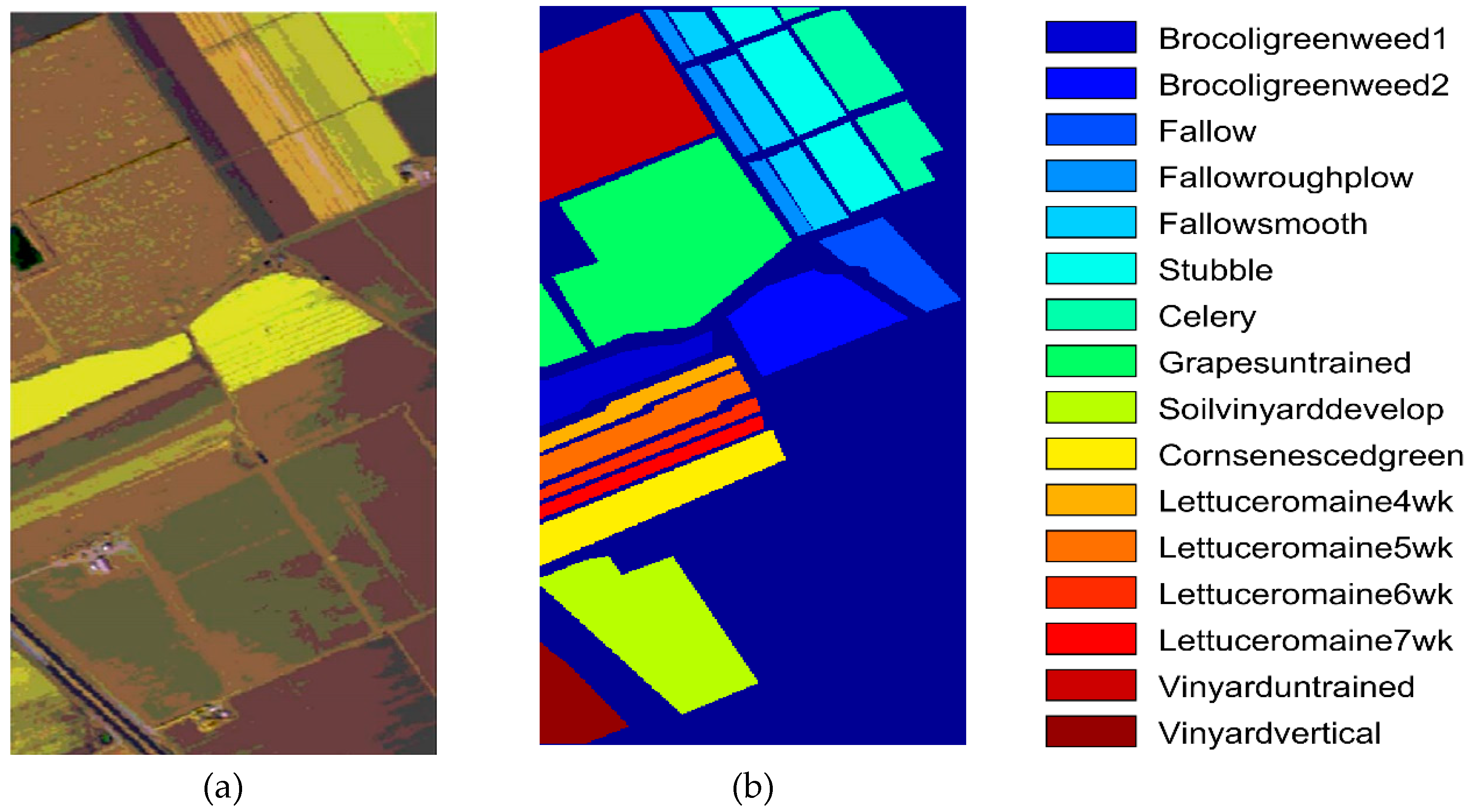
Figure 5.
Salinas dataset. (a) False color image. (b) Ground-truth.

Figure 6.
The classification results of Indian Pines dataset. (a) SVM. (b) SVM-SP (s = 5). (c) DPR-SVM-POS (m = 15, s = 5 and β = 0.9). (d) DPR-SVM-SP (s = 5 and β = 0.9).
Figure 6.
The classification results of Indian Pines dataset. (a) SVM. (b) SVM-SP (s = 5). (c) DPR-SVM-POS (m = 15, s = 5 and β = 0.9). (d) DPR-SVM-SP (s = 5 and β = 0.9).

Figure 7.
The classification results of Pavia University dataset. (a) SVM. (b) SVM-SP (s = 9). (c) DPR-SVM-POS (m = 15, s = 9 and β = 0.2). (d) DPR-SVM-SP (s = 9 and β = 0.2).
Figure 7.
The classification results of Pavia University dataset. (a) SVM. (b) SVM-SP (s = 9). (c) DPR-SVM-POS (m = 15, s = 9 and β = 0.2). (d) DPR-SVM-SP (s = 9 and β = 0.2).

Figure 8.
The classification results of Salinas dataset. (a) SVM. (b) SVM-SP (s= 15). (c) DPR-SVM-POS (m = 15, s = 15 and β = 0.9). (d) DPR-SVM-SP (s = 15 and β = 0.9).
Figure 8.
The classification results of Salinas dataset. (a) SVM. (b) SVM-SP (s= 15). (c) DPR-SVM-POS (m = 15, s = 15 and β = 0.9). (d) DPR-SVM-SP (s = 15 and β = 0.9).

Figure 9.
The classification results of four edge detection operator Robert, Sobel, Canny and Prewitt for different parameter combinations on three hyperspectral datasets. (Note: The color of the line represents the size of the OA accuracy. From dark blue to deep red, it means that the OA accuracy changes from small to greater. It can be clearly seen from (a)).

Figure 10.
The variation of the average classification accuracy with the increase of β. (a) Indian Pines. (b) Pavia University. (c) Salinas.
Figure 10.
The variation of the average classification accuracy with the increase of β. (a) Indian Pines. (b) Pavia University. (c) Salinas.

Figure 11.
The variation of the average classification accuracy with increase of segmentation scale s. (a) Indian Pines. (b) Pavia University. (c) Salinas.
Figure 11.
The variation of the average classification accuracy with increase of segmentation scale s. (a) Indian Pines. (b) Pavia University. (c) Salinas.

Figure 12.
The visualization of results in Table 7. (a) Indian Pines. (b) Pavia University. (c) Salinas.
Figure 12.
The visualization of results in Table 7. (a) Indian Pines. (b) Pavia University. (c) Salinas.


Table 1.
The main features of three hyperspectral datasets.
| Class | Indian Pines | Salinas | Pavia University |
|---|---|---|---|
| 16 | 16 | 9 | |
| band | 200 | 204 | 103 |
| Size | |||
| sensor | AVIRIS | AVIRIS | ROSIS |
| resolution | 20 m | 3.7 m | 1.3 m |
| sample | 10,249 | 54,129 | 42,776 |
Table 2.
Statistical results (mean and standard deviation in percent) of 10 independent classifications provided by SVM, SVM-SP, DPR-SVM-POS and DPR-SVM-SP on Indian Pines datasets with 5% labeled samples per class, s = 5 and β = 0.9.
Table 2.
Statistical results (mean and standard deviation in percent) of 10 independent classifications provided by SVM, SVM-SP, DPR-SVM-POS and DPR-SVM-SP on Indian Pines datasets with 5% labeled samples per class, s = 5 and β = 0.9.
| Classes | Train/Test | SVM | SVM-SP | DPR-SVM-POS | DPR-SVM-SP |
|---|---|---|---|---|---|
| Alfalfa | 3/43 | 8.37 ± 7.53 | 5.12 ± 13.83 | 61.17 ± 6.4 | 97.67 ± 0.00 |
| Corn-notill | 72/1356 | 61.97 ± 4.35 | 77.07 ± 6.20 | 93.16 ± 0.4 | 96.35 ± 0.11 |
| Corn-mintilla | 42/788 | 46.13 ± 2.77 | 59.49 ± 5.44 | 91.17 ± 0.7 | 92.57 ± 0.18 |
| Corn | 12/225 | 25.47 ± 5.59 | 32.36 ± 14.54 | 84.67 ± 0.6 | 75.47 ± 0.86 |
| Grass-pasture | 25/458 | 79.91 ± 3.74 | 85.33 ± 5.88 | 93.21 ± 0.2 | 90.46 ± 0.25 |
| Grass-trees | 37/693 | 94.14 ± 2.16 | 96.54 ± 2.31 | 99.86 ± 0 | 100.00 ± 0.00 |
| Grass-pasturemowed | 2/26 | 33.46 ± 14.51 | 60.77 ± 35.45 | 90 ± 2 | 100.00 ± 0.00 |
| Hay-windrowed | 24/454 | 94.47 ± 2.47 | 96.83 ± 3.32 | 98.94 ± 0.1 | 98.75 ± 0.11 |
| Oats | 1/19 | 4.74 ± 8.76 | 2.11 ± 6.32 | 60 ± 2.7 | 100.00 ± 0.00 |
| Soybean-notill | 49/923 | 64.60 ± 4.54 | 75.84 ± 5.41 | 91.51 ± 0.2 | 91.75 ± 0.19 |
| Soybean-mintill | 123/2332 | 80.64 ± 2.67 | 93.07 ± 1.81 | 98.81 ± 0 | 97.62 ± 0.06 |
| Soybean-clean | 30/563 | 37.90 ± 6.49 | 54.51 ± 12.23 | 85.61 ± 1.7 | 94.23 ± 0.12 |
| Wheat | 11/194 | 95.15 ± 2.84 | 98.19 ± 0.66 | 99.07 ± 0.3 | 99.07 ± 0.22 |
| Woods | 64/1201 | 95.50 ± 1.20 | 99.45 ± 1.00 | 97.94 ± 0.1 | 100.00 ± 0.00 |
| Building-grass-trees | 20/366 | 31.86 ± 6.19 | 38.36 ± 12.21 | 100 ± 0 | 99.76 ± 0.09 |
| Stone-steel-towers | 5/88 | 58.41 ± 7.52 | 84.77 ± 14.36 | 95.68 ± 0.5 | 90.34 ± 0.60 |
| OA | 71.04 ± 1.27 | 81.01 ± 2.27 | 95.09 ± 0.1 | 96.00 ± 0.04 | |
| AA | 57.05 ± 5.21 | 66.24 ± 8.81 | 90.05 ± 1.0 | 95.25 ± 0.17 | |
| κ | 66.54 ± 1.51 | 78.02 ± 2.68 | 94.39 ± 0.2 | 95.43 ± 0.05 |
Table 3.
Statistical results (mean and standard deviation in percent) of 10 independent classifications provided by SVM, SVM-SP, DPR-SVM-POS and DPR-SVM-SP on Pavia University datasets with 1% labeled samples per class, s =9 and β = 0.2.
Table 3.
Statistical results (mean and standard deviation in percent) of 10 independent classifications provided by SVM, SVM-SP, DPR-SVM-POS and DPR-SVM-SP on Pavia University datasets with 1% labeled samples per class, s =9 and β = 0.2.
| Classes | Train/Test | SVM | SVM-SP | DPR-SVM-POS | DPR-SVM-SP |
|---|---|---|---|---|---|
| Broccoligreenweed1 | 67/6564 | 85.85 ± 2.18 | 97.47 ± 0.95 | 96.86 ± 0.2 | 97.60 ± 0.02 |
| Broccoligreenweed2 | 187/18462 | 96.78 ± 1.07 | 99.30 ± 0.78 | 99.25 ± 0 | 99.90 ± 0.00 |
| Fallow | 21/2078 | 61.01 ± 4.05 | 72.51 ± 9.59 | 90.74 ± 0.9 | 93.43 ± 0.05 |
| Fallowroughplough | 31/3033 | 83.9 ± 4.57 | 87.44 ± 3.14 | 93.83 ± 0.1 | 94.95 ± 0.03 |
| Fallowsmooth | 14/1331 | 96.81 ± 3.34 | 99.71 ± 0.03 | 99.77 ± 0 | 97.92 ± 0.04 |
| Stubble | 51/4978 | 71.53 ± 4.55 | 78.97 ± 7.69 | 99.9 ± 0 | 98.88 ± 0.01 |
| Celery | 14/1316 | 77.31 ± 6.16 | 93.37 ± 4.46 | 99.02 ± 0 | 85.91 ± 0.08 |
| Grapesuntrained | 37/3645 | 82.56 ± 3.89 | 95.11 ± 2.66 | 92.15 ± 0.8 | 96.72 ± 0.03 |
| Soilvineyarddevelop | 10/937 | 99.63 ± 0.39 | 98.59 ± 0.04 | 99.26 ± 0 | 91.28 ± 0.11 |
| OA | 87.67 ± 1.06 | 93.92 ± 1.23 | 97.55 ± 0.1 | 97.70 ± 0.01 | |
| AA | 83.93 ± 3.35 | 91.39 ± 3.26 | 96.75 ± 0.2 | 95.18 ± 0.04 | |
| κ | 83.44 ± 1.48 | 91.82 ± 1.68 | 96.75 ± 0.1 | 97.06 ± 0.01 |
Table 4.
Statistical results (mean and standard deviation in percent) of 10 independent classifications provided by SVM, SVM-SP, DPR-SVM-POS and DPR-SVM-SP on Salinas datasets with 1% labeled samples per class, s = 15 and β = 0.9.
Table 4.
Statistical results (mean and standard deviation in percent) of 10 independent classifications provided by SVM, SVM-SP, DPR-SVM-POS and DPR-SVM-SP on Salinas datasets with 1% labeled samples per class, s = 15 and β = 0.9.
| Classes | Train/Test | SVM | SVM-SP | DPR-SVM-POS | DPR-SVM-SP |
|---|---|---|---|---|---|
| Brocoligreenweed1 | 21/1988 | 97.81 ± 0.93 | 100.00 ± 0.00 | 100 ± 0 | 100.00 ± 0.00 |
| Brocoligreenweed2 | 38/3688 | 99.31 ± 0.41 | 100.00 ± 0.00 | 100 ± 0 | 100.00 ± 0.00 |
| Fallow | 20/1956 | 92.32 ± 4.85 | 99.15 ± 2.68 | 98.53 ± 0 | 100.00 ± 0.00 |
| Fallowroughplow | 14/1380 | 98.52 ± 0.83 | 98.01 ± 0.05 | 84.47 ± 1 | 94.91 ± 0.07 |
| Fallowsmooth | 27/2651 | 96.68 ± 1.24 | 94.66 ± 0.04 | 82.72 ± 0.7 | 99.77 ± 0.01 |
| Stubble | 40/3919 | 99.55 ± 0.28 | 99.59 ± 0.01 | 99.8 ± 0 | 100.00 ± 0.00 |
| Celery | 36/3543 | 99.28 ± 0.20 | 99.86 ± 0.01 | 100 ± 0 | 100.00 ± 0.00 |
| Grapesuntrained | 113/11158 | 83.85 ± 5.19 | 93.37 ± 1.41 | 99 ± 0 | 98.01 ± 0.02 |
| Soilvinyarddevelop | 63/6140 | 98.95 ± 0.45 | 99.88 ± 0.06 | 100 ± 0 | 100.00 ± 0.00 |
| Cornsenescedgreen | 33/3245 | 86.63 ± 1.91 | 93.41 ± 5.71 | 97.9 ± 0 | 99.69 ± 0.00 |
| Lettuceromaine 4wk | 11/1057 | 87.71 ± 5.18 | 97.36 ± 4.75 | 94.93 ± 0.1 | 99.53 ± 0.00 |
| Lettuceromaine 5wk | 20/1907 | 98.00 ± 1.01 | 98.04 ± 0.69 | 85.82 ± 0.1 | 99.33 ± 0.02 |
| Lettuceromaine 6wk | 10/906 | 98.01 ± 0.80 | 98.14 ± 0.05 | 74.19 ± 0.2 | 98.04 ± 0.05 |
| Lettuceromaine 7wk | 11/1059 | 90.01 ± 2.85 | 96.81 ± 0.04 | 68.06 ± 0.1 | 96.22 ± 0.08 |
| Vinyarduntrained | 73/7195 | 58.65 ± 4.73 | 65.93 ± 9.04 | 98.49 ± 0 | 99.62 ± 0.01 |
| Vinyardvertical | 19/1788 | 93.87 ± 2.99 | 93.37 ± 4.89 | 100 ± 0 | 97.67 ± 0.03 |
| OA | 88.71 ± 0.88 | 92.81 ± 1.51 | 96.46 ± 0.01 | 99.16 ± 0.01 | |
| AA | 92.45 ± 2.12 | 95.47 ± 1.84 | 92.74 ± 0.1 | 98.92 ± 0.02 | |
| κ | 87.40 ± 0.97 | 91.97 ± 1.70 | 96.06 ± 0.01 | 99.06 ± 0.01 |
Table 5.
Comparison with other nine competitive methods on Indian Pines (IP), Pavia University (PU) and Salinas (SA) datasets. Train denotes the number of training samples per class (ratio or fixed number).
Table 5.
Comparison with other nine competitive methods on Indian Pines (IP), Pavia University (PU) and Salinas (SA) datasets. Train denotes the number of training samples per class (ratio or fixed number).
| Competitors | DPR-SVM-SP | OA Improvement | |||||
|---|---|---|---|---|---|---|---|
| Datasets | Train | OA | κ | OA | κ | % | |
| SP-SPR | IP | 10% | 97.24 | 97.00 | 97.14 ± 0.44 | 96.73 ± 0.51 | −0.1 |
| PU | 250 | 98.54 | 98.00 | 98.61 ± 0.21 | 98.13 ± 0.28 | 0.07 | |
| SP-MKL-LRR | IP | 10% | 96.90 | 96.40 | 97.14 ± 0.44 | 96.73 ± 0.51 | 0.24 |
| PU | 15% | 93.97 | 91.92 | 97.70 ± 0.01 | 97.06 ± 0.01 | 3.73 | |
| SBDSM | IP | 10% | 97.12 ± 0.41 | 97.00 ± 0.50 | 97.14 ± 0.44 | 96.73 ± 0.51 | 0.02 |
| PU | 250 | 97.33 ± 0.33 | 96.00 ± 0.50 | 98.61 ± 0.21 | 98.13 ± 0.28 | 1.28 | |
| SA | 1% | 99.37 ± 0.23 | 99.00 ± 0.20 | 99.16 ± 0.01 | 99.06 ± 0.01 | −0.21 | |
| SP-ELM | IP | 10% | 97.78 | 97.00 | 97.14 ± 0.44 | 96.73 ± 0.51 | −0.64 |
| PU | 300 | 98.17 | 98.00 | 98.95 ± 0.21 | 98.58 ± 0.28 | 0.78 | |
| MSP-SVMsub | IP | 15 | 84.01 | 82.00 | 86.72 ± 2.59 | 84.94 ± 2.89 | 2.71 |
| PU | 100 | 97.57 | 97.00 | 97.54 ± 0.89 | 96.68 ± 1.17 | −0.03 | |
| EMP-SP-SVM | PU | 50 | 91.64 ± 1.21 | - | 93.74 ± 1.47 | 91.81 ± 1.88 | 2.1 |
| SA | 50 | 94.01 ± 0.51 | - | 97.23 ± 0.71 | 96.92 ± 0.79 | 3.22 | |
| SoCRATE | IP | 5% | 98.18 | - | 96.00 ± 0.04 | 95.43 ± 0.05 | −2.18 |
| PU | 1% | 93.44 | - | 97.70 ± 0.01 | 97.06 ± 0.01 | 4.26 | |
| SA | 1% | 98.64 | - | 99.16 ± 0.01 | 99.06 ± 0.01 | 0.52 | |
| S-SAE | IP | 10% | 96.66 ± 0.66 | 96.19 ± 0.80 | 97.14 ± 0.44 | 96.73 ± 0.51 | 0.48 |
| PU | 5% | 96.66 ± 0.28 | 95.57 ± 0.40 | 98.81 ± 0.23 | 98.42 ± 0.30 | 2.15 | |
| IP | 30 | 94.62 | 93.83 | 95.52 ± 0.21 | 94.94 ± 0.12 | 0.9 | |
| SuperPCA | PU | 30 | 91.3 | 88.56 | 92.64 ± 1.23 | 89.91 ± 1.35 | 1.34 |
| SA | 30 | 98.97 | 98.86 | 98.12 ± 0.76 | 98.03 ± 0.01 | −0.85 | |
Table 6.
The best results (mean and standard deviation) obtained by using four operators on Indian Pines (IP), Pavia University (PU) and Salinas (SA) datasets.
Table 6.
The best results (mean and standard deviation) obtained by using four operators on Indian Pines (IP), Pavia University (PU) and Salinas (SA) datasets.
| Canny | Prewitt | Sobel | Robert | |||||||||
|---|---|---|---|---|---|---|---|---|---|---|---|---|
| OA(%) | β | s | OA(%) | β | s | OA(%) | β | s | OA(%) | β | s | |
| IP | 92.91 ± 0.09 | 0.9 | 7 | 93.75 ± 0.08 | 0.9 | 5 | 94.22 ± 0.09 | 0.7 | 5 | 96 ± 0.04 | 0.9 | 5 |
| PU | 97.86 ± 0.01 | 0.5 | 13 | 97.75 ± 0.01 | 0.4 | 11 | 97.59 ± 0.01 | 0.6 | 9 | 97.7 ± 0.01 | 0.2 | 9 |
| SA | 97.57 ± 0.01 | 0.9 | 17 | 99 ± 0.01 | 0.9 | 15 | 98.98 ± 0.01 | 0.9 | 13 | 99.16 ± 0.01 | 0.9 | 15 |
Table 7.
The variation of average classification accuracy (OA in percent) of three datasets with the increase of the number of training samples.
Table 7.
The variation of average classification accuracy (OA in percent) of three datasets with the increase of the number of training samples.
| Indian Pines | Pavia University | Salinas | |||||||||
|---|---|---|---|---|---|---|---|---|---|---|---|
| Training samples | SVM | SVM-SP | DPR-SVM-SP | Training samples | SVM | SVM-SP | DPR-SVM-SP | Training samples | SVM | SVM-SP | DPR-SVM-SP |
| 1% | 44.35 ± 9.20 | 45.58 ± 10.12 | 82.44 ± 2.96 | 1% | 86.88 ± 1.06 | 93.08 ± 1.53 | 97.68 ± 0.22 | 0.1% | 80.07 ± 2.41 | 84.93 ± 2.95 | 91.06 ± 1.93 |
| 2% | 63.31 ± 1.13 | 71.07 ± 2.15 | 89.13 ± 2.05 | 2% | 91.11 ± 0.50 | 97.35 ± 0.57 | 97.92 ± 0.37 | 0.2% | 82.65 ± 1.09 | 87.16 ± 2.29 | 93.96 ± 1.86 |
| 3% | 67.27 ± 1.09 | 75.00 ± 2.70 | 92.72 ± 1.01 | 3% | 92.22 ± 0.47 | 97.88 ± 0.42 | 98.66 ± 0.28 | 0.3% | 84.92 ± 1.51 | 90.16 ± 2.40 | 95.78 ± 0.69 |
| 4% | 69.25 ± 1.05 | 77.27 ± 1.70 | 94.29 ± 0.47 | 4% | 93.01 ± 0.32 | 98.35 ± 0.23 | 98.73 ± 0.20 | 0.4% | 85.31 ± 1.54 | 88.83 ± 3.09 | 96.46 ± 1.06 |
| 5% | 71.55 ± 1.39 | 80.59 ± 2.56 | 96.04 ± 0.89 | 5% | 93.36 ± 0.20 | 98.55 ± 0.11 | 98.81 ± 0.23 | 0.5% | 86.15 ± 1.02 | 91.87 ± 3.10 | 96.95 ± 0.90 |
| 6% | 73.18 ± 1.06 | 82.87 ± 2.09 | 96.26 ± 0.64 | 6% | 93.67 ± 0.28 | 98.56 ± 0.14 | 98.97 ± 0.18 | 0.6% | 86.70 ± 1.30 | 91.10 ± 2.25 | 97.05 ± 0.63 |
| 7% | 75.03 ± 0.51 | 83.51 ± 1.29 | 97.01 ± 0.30 | 7% | 93.78 ± 0.19 | 98.43 ± 0.21 | 99.19 ± 0.18 | 0.7% | 87.83 ± 0.71 | 91.84 ± 1.58 | 97.53 ± 0.77 |
| 8% | 75.89 ± 0.38 | 85.95 ± 1.92 | 96.87 ± 0.34 | 8% | 94.15 ± 0.24 | 98.79 ± 0.12 | 99.25 ± 0.15 | 0.8% | 87.87 ± 0.82 | 92.26 ± 1.53 | 97.41 ± 0.59 |
| 9% | 77.05 ± 0.61 | 86.77 ± 1.25 | 97.24 ± 0.53 | 9% | 94.26 ± 0.14 | 98.68 ± 0.17 | 99.22 ± 0.15 | 0.9% | 88.66 ± 0.79 | 92.52 ± 1.50 | 98.20 ± 0.50 |
| 10% | 77.79 ± 0.64 | 87.95 ± 1.69 | 97.14 ± 0.44 | 10% | 94.44 ± 0.08 | 98.88 ± 0.14 | 99.25 ± 0.15 | 1% | 89.23 ± 0.35 | 93.79 ± 1.19 | 99.12 ± 0.42 |
© 2019 by the authors. Licensee MDPI, Basel, Switzerland. This article is an open access article distributed under the terms and conditions of the Creative Commons Attribution (CC BY) license (http://creativecommons.org/licenses/by/4.0/).
Share and Cite
MDPI and ACS Style
Xie, F.; Lei, C.; Yang, J.; Jin, C. An Effective Classification Scheme for Hyperspectral Image Based on Superpixel and Discontinuity Preserving Relaxation. Remote Sens. 2019, 11, 1149. https://0-doi-org.brum.beds.ac.uk/10.3390/rs11101149
AMA Style
Xie F, Lei C, Yang J, Jin C. An Effective Classification Scheme for Hyperspectral Image Based on Superpixel and Discontinuity Preserving Relaxation. Remote Sensing. 2019; 11(10):1149. https://0-doi-org.brum.beds.ac.uk/10.3390/rs11101149
Chicago/Turabian StyleXie, Fuding, Cunkuan Lei, Jun Yang, and Cui Jin. 2019. "An Effective Classification Scheme for Hyperspectral Image Based on Superpixel and Discontinuity Preserving Relaxation" Remote Sensing 11, no. 10: 1149. https://0-doi-org.brum.beds.ac.uk/10.3390/rs11101149
Note that from the first issue of 2016, this journal uses article numbers instead of page numbers. See further details here.