Context Aggregation Network for Semantic Labeling in Aerial Images


1
School of Electronic Information, Wuhan University, Wuhan 430072, China
2
The CETC Key Laboratory of Aerospace Information Applications, Shijiazhuang 050081, China
*
Author to whom correspondence should be addressed.
Remote Sens. 2019, 11(10), 1158; https://0-doi-org.brum.beds.ac.uk/10.3390/rs11101158
Submission received: 23 April 2019
/
Revised: 13 May 2019
/
Accepted: 14 May 2019
/
Published: 15 May 2019
(This article belongs to the Section Remote Sensing Image Processing)
Abstract
:Semantic labeling for high resolution aerial images is a fundamental and necessary task in remote sensing image analysis. It is widely used in land-use surveys, change detection, and environmental protection. Recent researches reveal the superiority of Convolutional Neural Networks (CNNs) in this task. However, multi-scale object recognition and accurate object localization are two major problems for semantic labeling methods based on CNNs in high resolution aerial images. To handle these problems, we design a Context Fuse Module, which is composed of parallel convolutional layers with kernels of different sizes and a global pooling branch, to aggregate context information at multiple scales. We propose an Attention Mix Module, which utilizes a channel-wise attention mechanism to combine multi-level features for higher localization accuracy. We further employ a Residual Convolutional Module to refine features in all feature levels. Based on these modules, we construct a new end-to-end network for semantic labeling in aerial images. We evaluate the proposed network on the ISPRS Vaihingen and Potsdam datasets. Experimental results demonstrate that our network outperforms other competitors on both datasets with only raw image data.
1. Introduction
For aerial images, semantic labeling means assigning each pixel a category label, which is also known as semantic segmentation in the computer vision field. In nature, it is a multi-category classification problem which needs to classify every pixel in the aerial image [1,2,3]. This characteristic makes it more sophisticated than binary classification problems, like building extraction and road extraction. Besides, different from digital photos widely used in the computer vision field, objects present large scale variations and compose complex scenes in aerial images, especially in urban areas. They consist of many kinds of objects, like buildings, vegetation, trees, etc. Buildings have varying sizes, cars are tiny, while trees are interwoven with vegetation. These properties make the semantic labeling task more difficult. It is a necessary task in aerial image interpretation in spite of its difficulty and becomes the basis for following applications, including land-use analysis, environmental protection, urban change detection, urban planning, and so on [4,5,6,7,8].
Regarding this task, researchers have proposed numerous methods to accomplish it, which could be divided into two types, traditional methods and Convolutional Neural Networks (CNNs) methods.
Traditional methods mainly consist of two independent parts, i.e., feature extraction and classification algorithms. Certain types of features are extracted from a small patch in the aerial image, then sent to classifier to determine its category. Features are generally constructed manually, including Scale Invariant Feature Transform (SIFT) [9], Histogram of Oriented Gradients (HOG) [10], and Features from Accelerated Segment Test (FAST) [11]. These hand-crafted features have their own characteristics in specific conditions while cannot handle general situation well. Researchers need to choose suitable features for their specific situation carefully, otherwise they have to design a custom feature. Classifiers used here are mostly regular machine learning algorithms. K-means [12], Support vector machines [13], and Random forests [14] are widely adopted. However, high resolution aerial images, especially urban areas, have complex scenes and objects in different categories present similar appearances. So these traditional methods do not get satisfying results for this task.
In recent years, CNNs have shown dominant performance in the image processing field. It can construct features automatically from massive image data and implement feature extraction and classification simultaneously, which is called an end-to-end method. It presents great performance in the image classification task [15]. Many classic networks for image classification have been proposed, such as VGG [16], ResNet [17], and DenseNet [18].
Due to the strong recognition ability and feature learning characteristic, CNNs have been introduced to the semantic labeling field. Many CNNs models based on image patch classification have been designed for this task [19,20,21,22,23]. The general procedure is cropping a small patch from original large image by sliding window, then classifying this patch with CNNs. This method gets improved performance compared with traditional methods owing to superior feature expressive ability, but loses structural information due to the regular patch partition. Besides, it requires large computational cost because of the enormous iteration steps needed by sliding window method [24]. As an improvement, researchers try to use a structural segmentation algorithm, like superpixel segmentation methods, to generate patches with irregular shapes and retain more structural information [25,26]. Then they employ CNNs models to extract features and classify patches. However, this method still makes use of segmentation algorithms that are decoupled from CNN models, thus taking a risk of commitment to premature decisions.
To overcome the difficulty, Fully Convolutional Networks (FCN) [27] have been proposed. FCN removes fully connected layers in VGG and outputs the probability map directly. Afterwards, it upsamples the probability map to the same size with original input image. In some sense, FCN discards the segmentation part and generates a semantic labeling outcome as a natural result of pixel-level classification. As a result, FCN can deal with irregular boundaries and get more coherent results than patch-based classification methods.
Although FCN achieves much better performance than other models [20,21], there still exist two limitations. Firstly, the feature map size is greatly reduced due to consecutive downsample operations, so the spatial resolution of the final feature map is largely reduced. This means a great deal of information is lost, which makes it difficult to recover details from the small and coarse feature map. Lastly, the semantic labeling result misses plenty of details and seems vague locally. Secondly, it uses features extracted by the backbone network directly, without exploiting features efficiently. This makes FCN weak in capturing multi-scale features and recognizing complicated scenes. Hence, for objects with multiple scales, it cannot recognize them well. This problem is more severe in aerial images due to the large scale variations, complex scenes, and fine-structured objects.
To remedy the first problem, researchers either generate feature map with higher resolution, or take advantage of shallow layer features more efficiently. For instance, DeconvNet [28] uses consecutive unpooling and deconvolution layers to restore feature map resolution step wise. It adopts encoder–decoder architecture, in fact. SegNet [29] records a pooling index in the encoder part, then utilizes pooling index information to perform non-linear upsampling in the decoder part and get more accurate location information. This eliminates the need for upsampling in a learning way. U-Net [30] proposes a similar encoder–decoder model and introduces low-level features to improve final result during decoder stage. FRRN [31] designs a two-stream network. One stream carries information at the full image resolution to keep precise boundaries. The other stream goes through consecutive pooling operations to get robust features for recognition. RefineNet [32] devises a multi-path refinement network. It exploits information along the downsampling process to perform high resolution predictions with long-range residual connections.
For the other problem, researchers try to exploit features extracted by CNN more extensively. PSPNet [33] exploits global context information by different-region-based context aggregation through spatial pyramid pooling. DeepLab [34,35] uses parallel dilated convolutional operations to aggregate multi-scale features and robustly segment objects at multiple scales. GCN [36] validates the effectiveness of large convolution kernel and applies global convolution operation to capture context information. EncNet [37] introduces context encoding module, which captures the semantic context of scenes and selectively highlights class-dependent feature maps to capture context information.
In this paper, we introduce a novel end-to-end network for semantic labeling in aerial images, which can handle problems mentioned above efficiently. It is an encoder–decoder-like architecture, with efficient context information aggregation and attention-based multi-level feature fusion. Specifically, we design a Context Fuse Module (CFM), which is composed of parallel convolutional layers with kernels of different sizes and a global pooling branch. The former is used to aggregate context information with multiple receptive fields. The latter is used to introduce global information which has been proved efficient in recent works [33,35]. We also propose an Attention Mix Module (AMM), which utilizes a channel-wise attention mechanism to combine multi-level features and selectively emphasizes more discriminative features. We further employ a Residual Convolutional Module (RCM) to refine features in all feature levels. Based on these modules, we construct a new end-to-end network for semantic labeling in aerial images. We evaluate the proposed network on ISPRS Vaihingen and Potsdam datasets. Experimental results demonstrate that our network outperforms other state-of-the-art CNN-based models and top methods on the benchmark with only raw image data.
In summary, our contributions are:
- We design a Context Fuse Module to exploit context information extensively. It is composed of parallel convolutional layers with different size kernels to aggregate context information with multiple receptive fields, and a global pooling branch to introduce global information.
- We propose an Attention Mix Module, which utilizes channel-wise attention mechanism to combine multi-level features and selectively emphasizes more discriminative features for recognition. We further employ a Residual Convolutional Module to refine features in all feature levels.
- Based on these models, we construct a new end-to-end network for semantic labeling in aerial images. We evaluate the proposed network on ISPRS Vaihingen and Potsdam datasets. Experimental results demonstrate that our network outperforms other state-of-the-art CNN-based models and top methods on the benchmark with only raw image data, without using digital surface model information.
- We make our PyTorch-based implementation of the proposed model publicly available at https://github.com/Spritea/Context-Aggregation-Network.
2. Methods
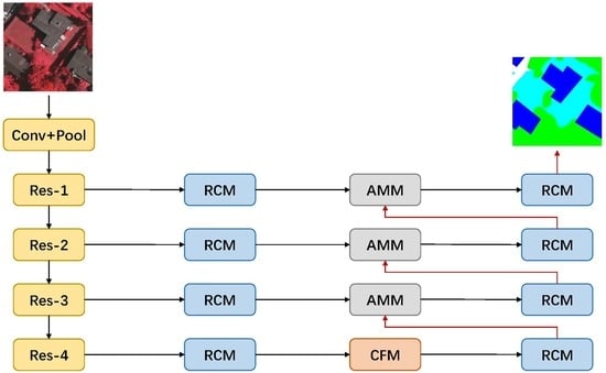
We would detail various parts of the end-to-end network for semantic labeling in this section. We first illustrate the proposed Context Fuse Module (CFM), Attention Mix Module (AMM), and Residual Convolutional Module (RCM) in detail. Then we introduce the Context Aggregation Network (CAN) based on these models for semantic labeling in aerial images. Figure 1 shows the overall framework of CAN.
2.1. Context Fuse Module
In the task of semantic labeling, context information is critical. Due to large scale variations and complex scenes in aerial images, context information is essential for accurate semantic labeling. For example, PSPNet [33] applies spatial pyramid pooling to fuse features in different levels. Ref. [38] uses cascaded dilated convolutional layers to enlarge the receptive field without extra parameters. DeepLabv3 [35] employs parallel dilated convolutional layers with global pooling layers to combine multi-scale features. However, spatial pyramid pooling [33] is a downsample operation in nature and would lose some detail information. Dilated convolution [34] would result in gridding effect [39] and generate feature map with checkerboard pattern. To overcome this, we propose the CFM block to aggregate features with different receptive fields and global context information efficiently.
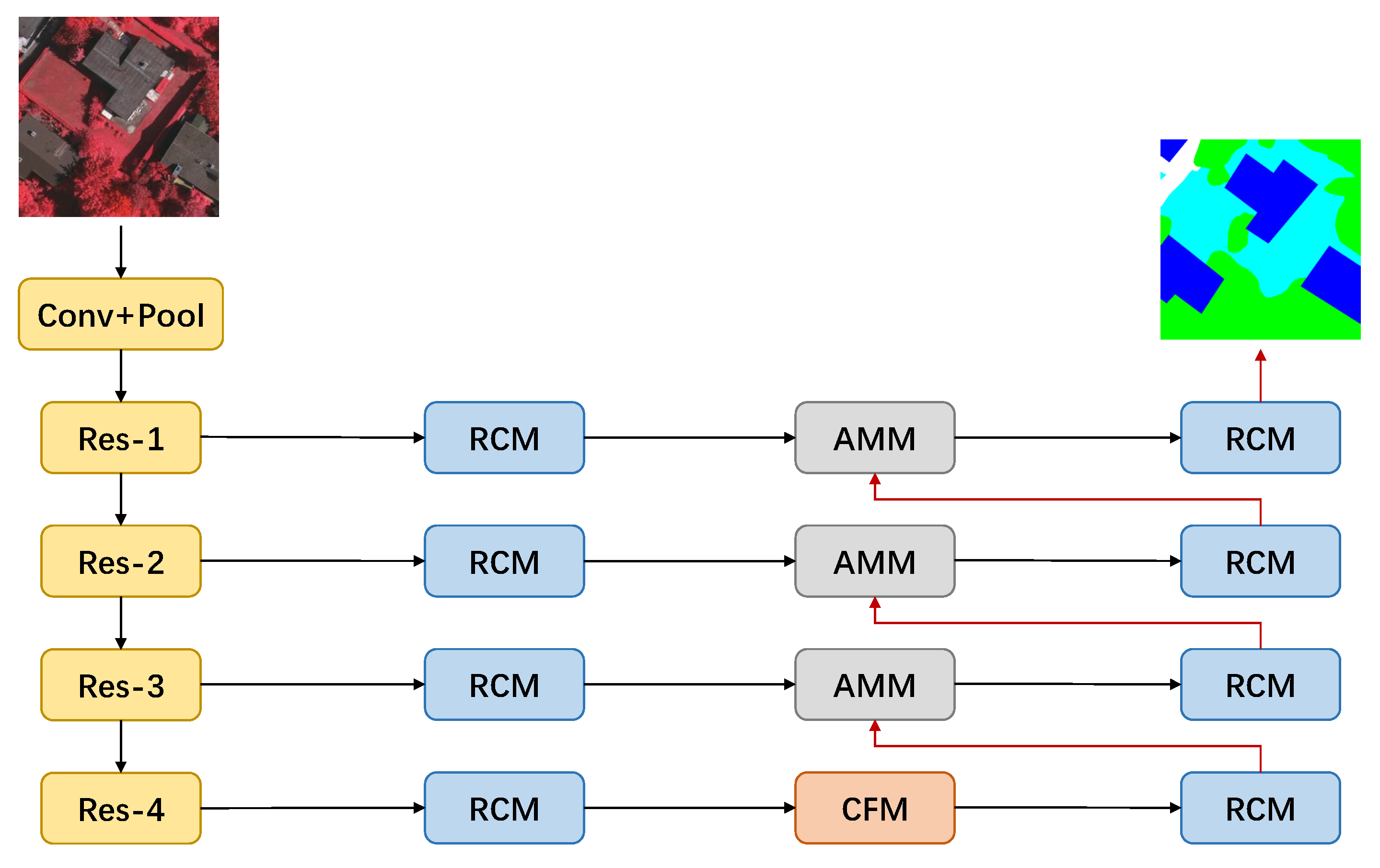
Our CFM block mainly consists of two parts, as shown in Figure 2. Part A is a parallel convolutional block, containing 4 branches with different convolutional kernel sizes. Part B is a global pooling branch to introduce gloabl context information.
Parallel Convolutional Block. Parallel Convolutional Block is composed of 4 convolutional branches with different kernel sizes, i.e., {3, 7, 11, 15}. Each branch has two convolutional layers to extract features generated by backbone network. We also use batch normalization [40] to reduce internal covariate shift and use ReLU [41] as activation function. Different with ASPP in DeepLabv3 [35], we use a regular convolutional layer (solid kernel), rather than a dilated convolutional layer (zero-padding kernel). In this way, we prevent feature maps from having the gridding effect and get more consistent results. For features extracted by each convolutional branch, we concatenate them together to fuse features with different receptive fields.
As for convolutioinal kernel sizes, the largest one is a 15 × 15 convolutional kernel. The reason is the last convolutional layer of ResNet [17] backbone network outputs a 1/32 input image size feature map. Input image size here is 512 × 512, and the last feature map size is 16 × 16. Then this 15 × 15 convolutional branch becomes the global convolution [36], and shares the same benefit with pure classification. This increases network’s ability to recognize complex objects. Kernel sizes could be adjusted according to input image size. Besides, since the last fature map is small, these large kernel convolutional layers just increase subtle extra computation cost.
Global Pooling Branch. Global pooling has been proved efficient in recent works [33,35,42]. PSPNet [33] utilizes global pooling in pyramid pooling module to introduce global context information. DeepLabv3 [35] adopts global pooling as a supplement to astrous spatial pyramid pooling. ParseNet [42] employs extra global context to clarify local confusion and smooth segmentation.
We also adopt global average pooling to introduce global information. In this branch, feature maps pass through a global average pooling layer to capture global context, then a 1 × 1 convolutional layer to perform channel reduction. Final feature maps are then upsampled and concatenated with Parallel Convolutional Block output.
The whole procedure of CFM block could be expressed as:
where stands for a series of operations in a global pooling branch, and means stacked layers in one branch of convolutional parallel block whose kernel size is equal to i. ⊕ and denote single and consecutive concatenation operations.
In this way, Parallel Convolutional Block aggregates multi-scale information via convolutional layers with different kernel sizes, and Global Pooling Branch captures global context information through a global pooling layer. As a result, CFM block generates features containing multi-scale information and global context information. These features are necessary for semantic labeling in aerial images due to the large scale variations and complex scenes.
2.2. Attention Mix Module
For the semantic labeling backbone network, deep layer features contain high-level semantic information with low spatial resolution, while shallow layer features embrace low-level structural information with high spatial resolution. To acquire more accurate location information, many works combine shallow layer features with deep ones. FCN [27] uses skip connections to add shallow layer features to deep layer features. U-Net [30] concatenates shallow layer features with deep ones step by step to perform feature fusion. DeepLabv3+ [43] conducts channel reduction on one shallow layer feature and concatenates it with one deep.
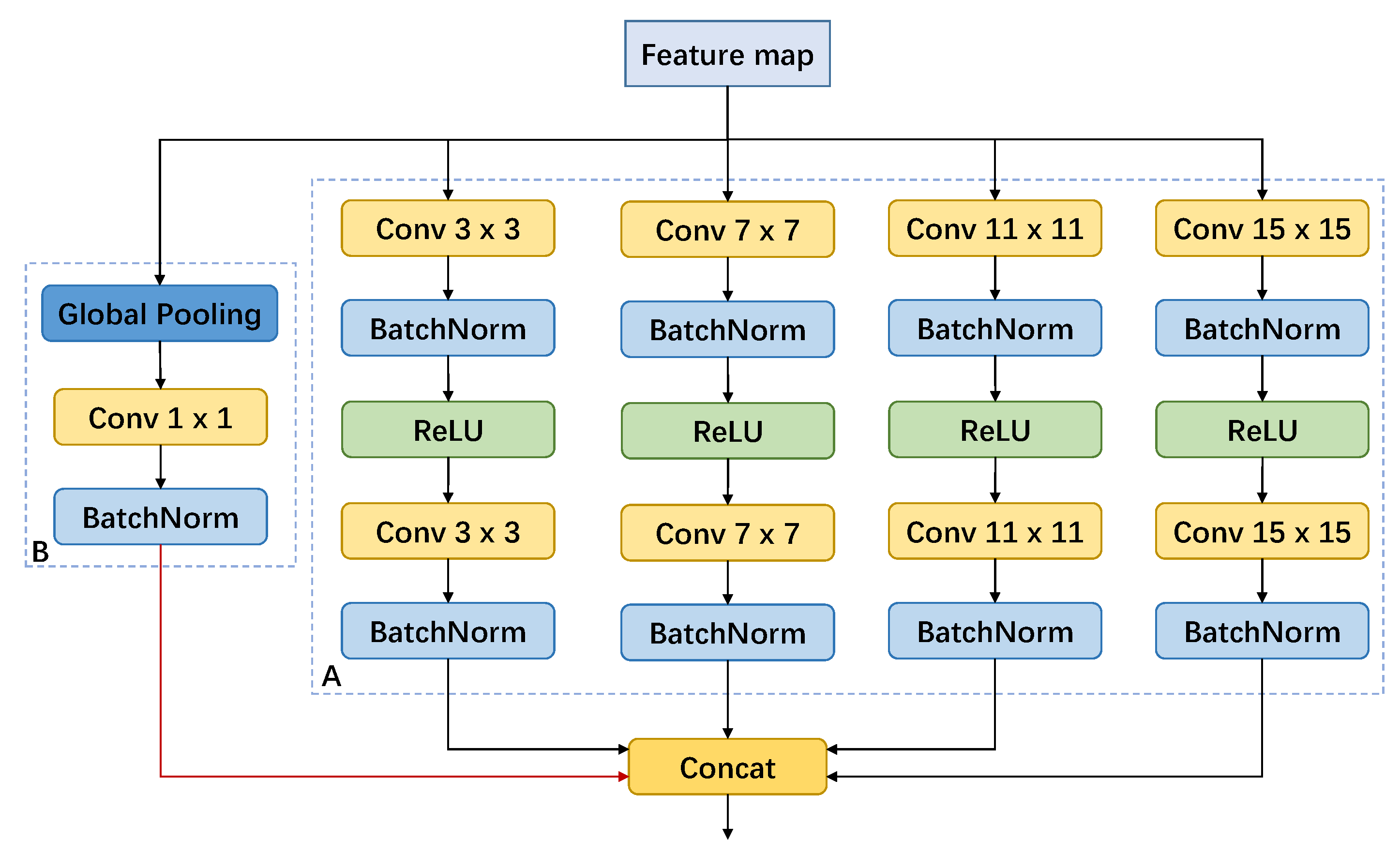
However, they either add them directly [27] or concatenate them together [30,43], without considering differences among channels. Inspired by SENet [44], we argue that the interdependence between channels of convolutional features matters. Therefore, we design the AMM block to combine low-level features and high-level features, as Figure 3 shows.
For a trivial semantic labeling network, like FCN [27], the multi-level feature fusion could be expressed as:
where denotes high-level features (usually upsampled), and denotes low-level features. They are added per-element and F is the sum.
For our proposed AMM, the future fusion process could be described with Equations (3) and (4).
where ⊕ means concatenation operation and includes convolution, batch normalization and ReLU activation operations. is the corresponding output before global pooling.
where means global pooling operation, and F is the final output of AMM block.
Specifically, low-level features and high-level features are concatenated together, then a 3 × 3 convolutional layer is used to perform channel reduction. After that, the feature map is reduced to 1 × 1 size with global average pooling and becomes a vector. The vector is multiplied with itself as a channel attention weight. In this way, we emphasize more discriminative feature channels and suppress less discriminative ones. Finally, we add low-level feature to it directly to perform an explicit fusion, which makes this module a residual-like structure and share similar benefits with residual block [17]. Hence we fuse multi-level features more adaptively and get features with higher recognition ability.
2.3. Residual Convolutional Module
Since the backbone networks are originally used in classification task, researchers add extra layers to adapt them to semantic labeling task. RefineNet [32] applies residual unit to perform feature adaptation. GCN [36] utilizes residual unit to refine boundaries and get more accurate contours. DFN [45] uses residual unit to refine features. Residual unit in these models are essentially variants of Residual Block in ResNet [17].
According to deep residual learning [17], we explicitly let these layers fit a residual mapping, instead of making few stacked layers directly fit a desired underlying mapping. This could be defined as:
where x is the input, is the desired underlying mapping, and is the new residual mapping we let stacked nonlinear layers fit. The original mapping becomes
As demonstrated in deep residual learning [17], it is easier to optimize the residual mapping than to optimize the original mapping. So residual unit not only performs feature refinement and adaptation, but also makes network training easier.
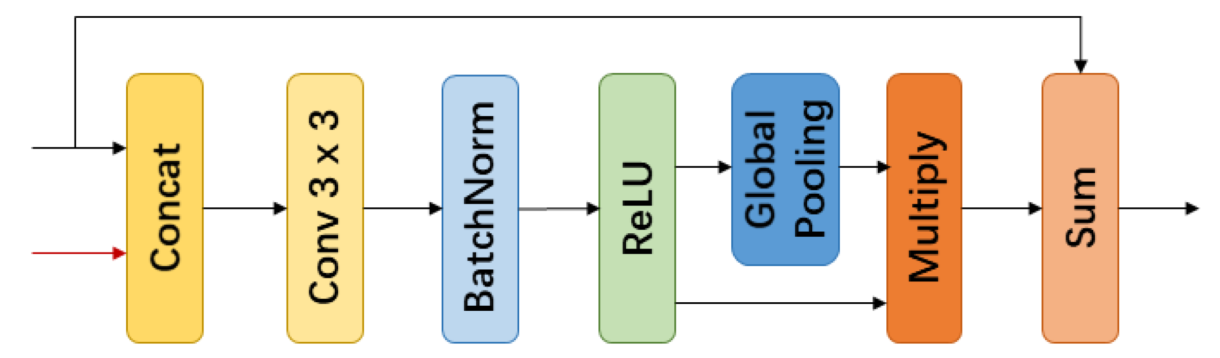
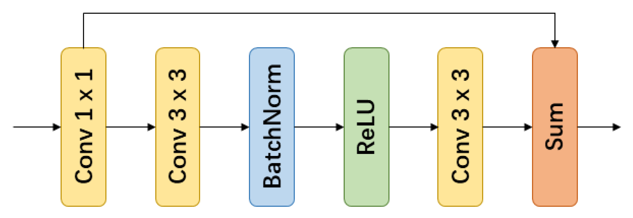
Therefore, we employ RCM block to implement this function. As presented in Figure 4, RCM block consists of a 1 × 1 convolutional layer and a residual-like block. The 1 × 1 convolutional layer unifies channel number in all levels to 512. Residual unit performs feature adaption and refinement. Furthermore, this residual unit contains several convolutional layers, so adding it makes the network deeper. Hence, we argue this module also strengthen the network’s ability to capture sophisticated features.
2.4. Context Aggregation Network
Based on proposed modules, we build the CAN model for semantic labeling in aerial images. As Figure 1 shows, this is an encoder–decoder like architecture [30]. ResNet [17] is adopted as the backbone network due to its strong feature extraction ability. For outputs of every stage in ResNet, they go through RCM block for feature adaption and refinement. Then the last layer’s feature map, which contains rich high-level semantic information, is feed into CFM block to capture and aggregate multi-scale features. After that, different-level feature maps generated in multi stages of backbone network are combined through AMM block. These combined features are refined by RCM block and then the network outputs final semantic labeling result.
For the network output, denotes the j-th pixel in the i-th image, and denotes the network output before softmax at pixel . The probability of the pixel belonging to the k-th category calculated with softmax function could be denoted as:
where . K is the number of object classes.
Then we use normalized cross entropy loss as the optimization objective, which is:
where g is ground truth, means CAN model parameters, M is mini-bath size, N is the number of pixels in one image, K is the number of object classes. is an indicative function which takes 1 when and takes 0 otherwise.
3. Results and Analysis
We evaluate our proposed CAN model on two public datasets: the ISPRS Vaihingen dataset and ISPRS Potsdam dataset. We first introduce the datasets and preprocess method. Then we present model training details and metrics used in experiments. Finally, we evaluate our network on the datasets and compare it with other state-of-the-art deep learning models and leading benchmark methods.
3.1. Experimental Settings
3.1.1. Dataset Description
ISPRS Vaihingen Dataset. This is a benchmark dataset of ISPRS 2D semantic labeling challenge in Vaihingen [46]. Vaihingen is a relatively small village with many detached buildings and small multi story buildings. It contains 3-band IRRG (Infrared, Red, and Green) image data, corresponding DSM (Digital Surface Model) and NDSM (Normalized Digital Surface Model) data. There are 33 images of about 2500 × 2000 pixels at a GSD (Ground Surface Distance) of about 9 cm. All images have corresponding ground truth images. There are 5 labeled categories: impervious surface, building, low vegetation, tree, car. Images in this dataset are acquired using an Intergraph/ZI DMC (Digital Mapping Camera) by the company RWE Power. The flying height above ground is 900 m. They are true ortho photos. Note that for proposed model and other deep learning models, only 3-band IRRG images are used without DSM and NDSM data in this dataset. The reason why DSM and NDSM data are not used is to explore the CNN-based model ability of semantic labeling in aerial images based on images purely. It would expand the application scope of our model, especially when DSM data is unavailable, which is often met in practical situation.
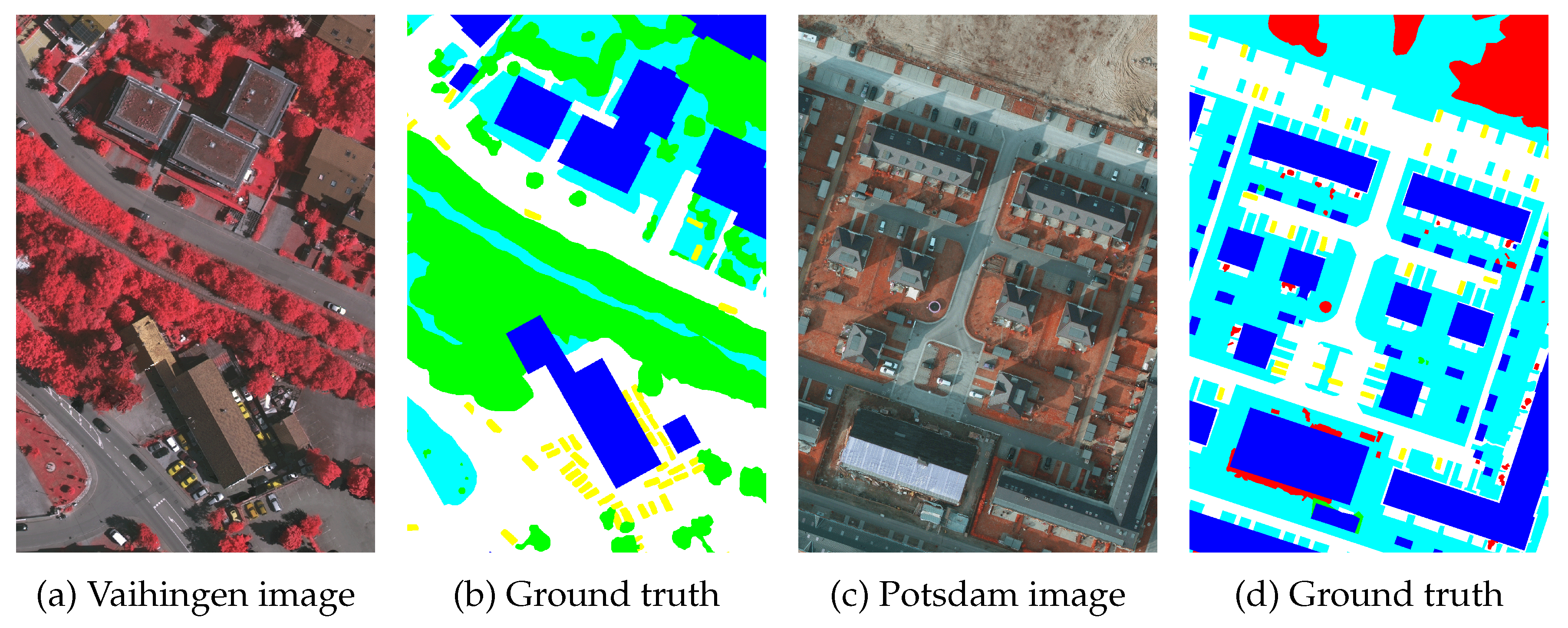
ISPRS Potsdam Dataset. This is another benchmark dataset of ISPRS 2D semantic labeling challenge in Potsdam [46]. Potsdam shows a typical historic city with large building blocks, narrow streets, and dense settlement structure. It contains 4-band IRRGB (Infrared, Red, Green, Blue) image data, corresponding DSM and NDSM data. There are 38 images of 6000 × 6000 pixels at a GSD of about 5 cm. All images have corresponding ground truth images. There are 5 labeled categories which are same with ISPRS Vaihingen dataset. Note that for proposed model and other deep learning models, only 3-band IRRG images extracted from 4-band IRRGB images are used without DSM and NDSM data. The reason why we choose Infrared, Red, and Green band data is mainly for consistency with the ISPRS Vaihingen dataset. Besides, this is also for fair comparison with models that use IRRG data only, like RIT_2 [47]. Figure 5 shows samples of ISPRS Vaihingen dataset and Potsdam dataset.
3.1.2. Dataset Preprocess
We conduct two kinds of evaluations, local evaluation and benchmark evaluation, of each dataset for comprehensive comparison, similar with [48]. Local evaluation is comparing proposed model with other state-of-the-art deep learning models. Online evaluation is comparing proposed model with leading benchmark models.
For local evaluation in ISPRS Vaihingen dataset, we randomly choose 23 images as the training set, and the other 10 images as the test set. For corresponding benchmark evaluation, we follow the data partition way in benchmark, i.e., 16 training images and 17 test images, for comparision with other benchmark models. For local evaluation in the ISPRS Potsdam dataset, we randomly choose 18 images as the training set due to the much larger image size than the Vaihingen dataset (6000 × 6000 v.s. 2500 × 2000), and the rest as the test set. For corresponding benchmark evaluation, we also follow the data partition way in benchmark, which selects 24 images as the training set and 14 as the test set. Note that for local evaluation in both datasets, we use full label images as ground truth images to set a higher standard and get more accurate results. For benchmark evaluation, we use eroded label images to be consistent with these benchmark methods.
Due to the GPU memory limit, original large training images are cropped with overlap 100 pixels to 512 × 512 pixels patches. Test images are cropped to same size patches without overlap. Since the datasets are small for deep learning methods, we apply horizontal flipping, vertical flipping, and rotation every 90 to augment the training set. We also resize original large images with a factor of and crop them to enlarge the training set.
3.1.3. Training Details
All experiments are conducted with PyTorch framework. We use the ResNet-50 [17] model weights pretrained on ImageNet [15] dataset. The context aggregation network is trained on two Titan V GPUs, with 12 GB memory per GPU. The total batch size is set to 12. Stochastic gradient descent (SGD) with momentum is adopted to train this network. Momentum and weight decay are set as 0.99 and 0.0005 respectively. The initial learning rate is set as 0.001. We apply step learning rate strategy to adjust learning rate, which reduces the learning rate by a factor of 0.1 every 50 epochs. This could be formulated as:
where is defined as:
For proposed model and comparing deep learning methods, we train them for 150 epochs in our experiment to make sure these networks converge. Note that only 3-band IRRG images are used in training process without DSM and NDSM data for both datasets, as explained in Section 3.1.1.
3.1.4. Metrics
To assess model performances comprehensively, we use three metrics: F1 score (F1), overall pixel accuracy (OA) and intersection over union (IoU). F1 is defined as:
OA is defined as
where are the number of true positive, false positive, true negative, false negative separately. IoU is defined as:
where is the prediction pixels set and is the ground truth pixels set. ∩ and ∪ mean the intersection and union set respectively. denotes the number of pixels in the intersection or union set.
Besides, we use precision-recall (PR) curve to assess the relation between precision and recall for each category. To be specific, we regard the multi-class classification problem as multiple binary classification problems. We adopt different thresholds from 0 to 1 to predicted score map of one category. Then we get several precision values with corresponding recall values and plot the PR curve of this category.
3.2. Local Evaluation
To compare proposed model with other deep learning models, we conduct comprehensive local evaluation. Deep learning models for comparison including FCN-8s [27], GCN [36], FRRN-B [31], DeepLabv3 [35], and DeepLabv3+ [43]. They are all typical deep learning models for semantic labeling (a.k.a. semantic segmentation) task.
FCN [27] is the first one dealing with this task with proposed fully convolutional network. GCN [36] utilizes large convolutional kernel to improve segmentation performance. FRRN [31] designs two information streams to combine high resolution feature maps with low resolution ones. DeepLabv3 [35] adopts astrous spatial pyramid pooling module with global pooling operation to extract high resolution feature maps. DeepLabv3+ [43] introduces low-level features to refine high-level features. Among them, DeepLabv3+ [43] is the most advanced model and achieves state-of-the-art performance on public dataset. These models only use IRRG images as input, without DSM or NDSM data.
3.2.1. Vaihingen Local Evaluation
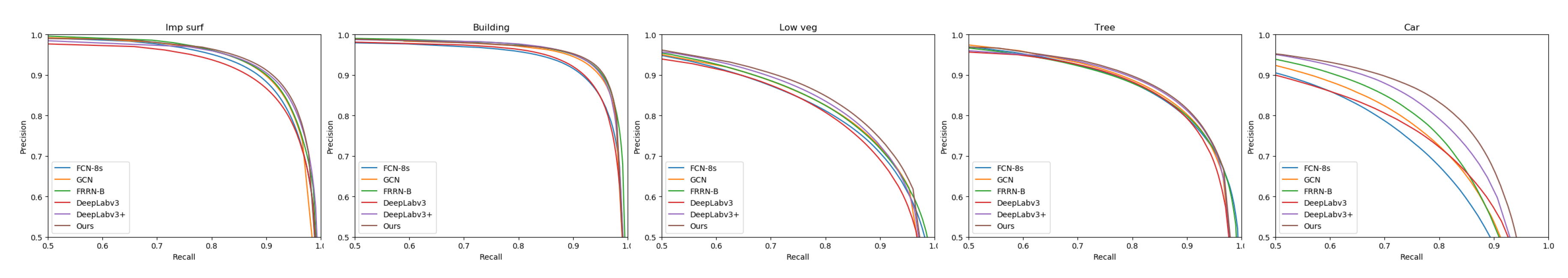
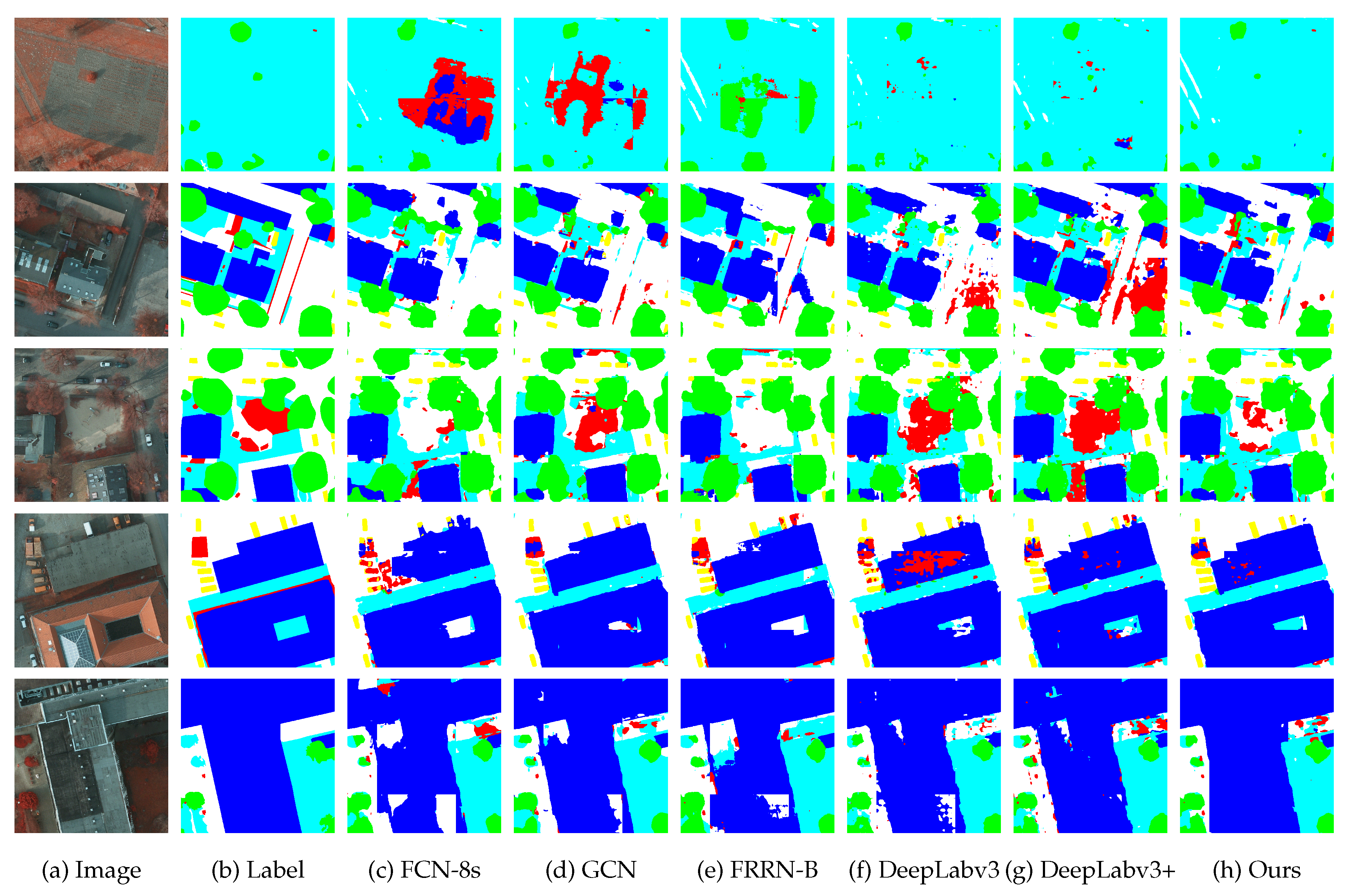
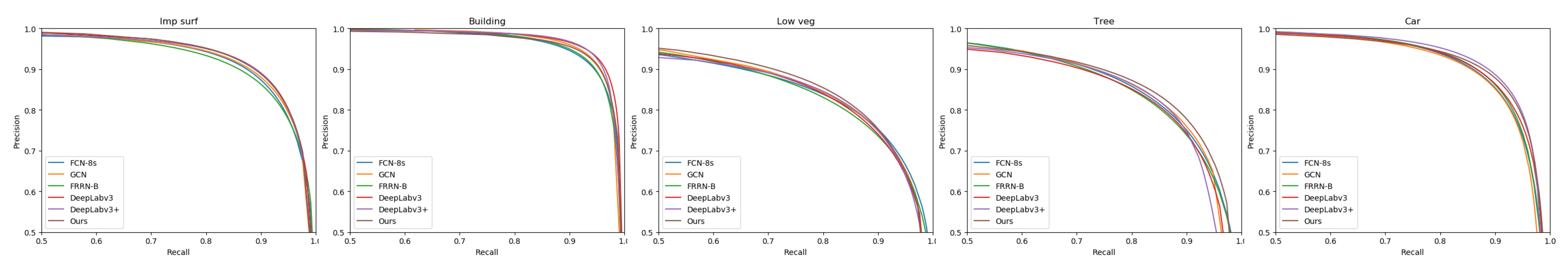
We first carry out local evaluation on the ISPRS Vaihingen dataset. Figure 6 presents visual results. Figure 7 exhibits PR curves for each category. Table 1 shows results in detail. The local evaluation result shows our proposed CAN model outperforms other state-of-the-art deep learning models significantly on Vaihingen dataset.
3.2.2. Potsdam Local Evaluation
We then conduct local evaluation on ISPRS Potsdam dataset. Figure 8 presents visual comparisons. Figure 9 exhibits PR curves for each category. Table 2 shows results in detail. The local evaluation result shows our proposed CAN model also outperforms other state-of-the-art deep learning models on the Potsdam dataset.
3.3. Benchmark Evaluation
To further prove proposed model’s effectiveness, we compare it with other leading benchmark models. SVL [49] is a series of baseline methods implemented by the challenge organizer. It utilizes SVL features [50] and Adaboost-based classifier for this task. SVL_3 does not apply Conditional Random Field (CRF) to refine segmentation result, while SVL_6 does. UZ_1 [51] is a CNN-based encoder–decoder-like model with deconvolution layers as decoder. ADL_3 [20] uses features from CNN and handcraft and random forest as classifier. It also applies CRF as a post-processing method. DST_2 [52] adopts a hybrid FCN architecture and CRF to deal with this task. DLR_8 [53] combines FCN [27], SegNet [29], and VGG [16] to tackle this problem. It further uses edge information to improve result. RIT_2 [47] adopts two SegNet models [29] trained with multimodal data and fuses them later. KLab_2 [54] employs synthetic multispectral imagery to initialize the CNN model and gets better result. CASIA [48] uses an encoder–decoder architecture-based CNN model with dilated convolutions. CASIA [48] has achieved state-of-the-art result among all published publicly methods on Vaihingen dataset. Note that all methods except KLab_2 [54] and CASIA [48] employ DSM data to improve their performance.
3.3.1. Vaihingen Benchmark Evaluation
We conduct benchmark evaluation on ISPRS Vaihingen dataset. Figure 10 shows visual results. Table 3 shows results in detail. The benchmark evaluation result shows our proposed CAN model outperforms other top methods, including CASIA [48] model, which is the best model publicly published, on Vaihingen dataset.
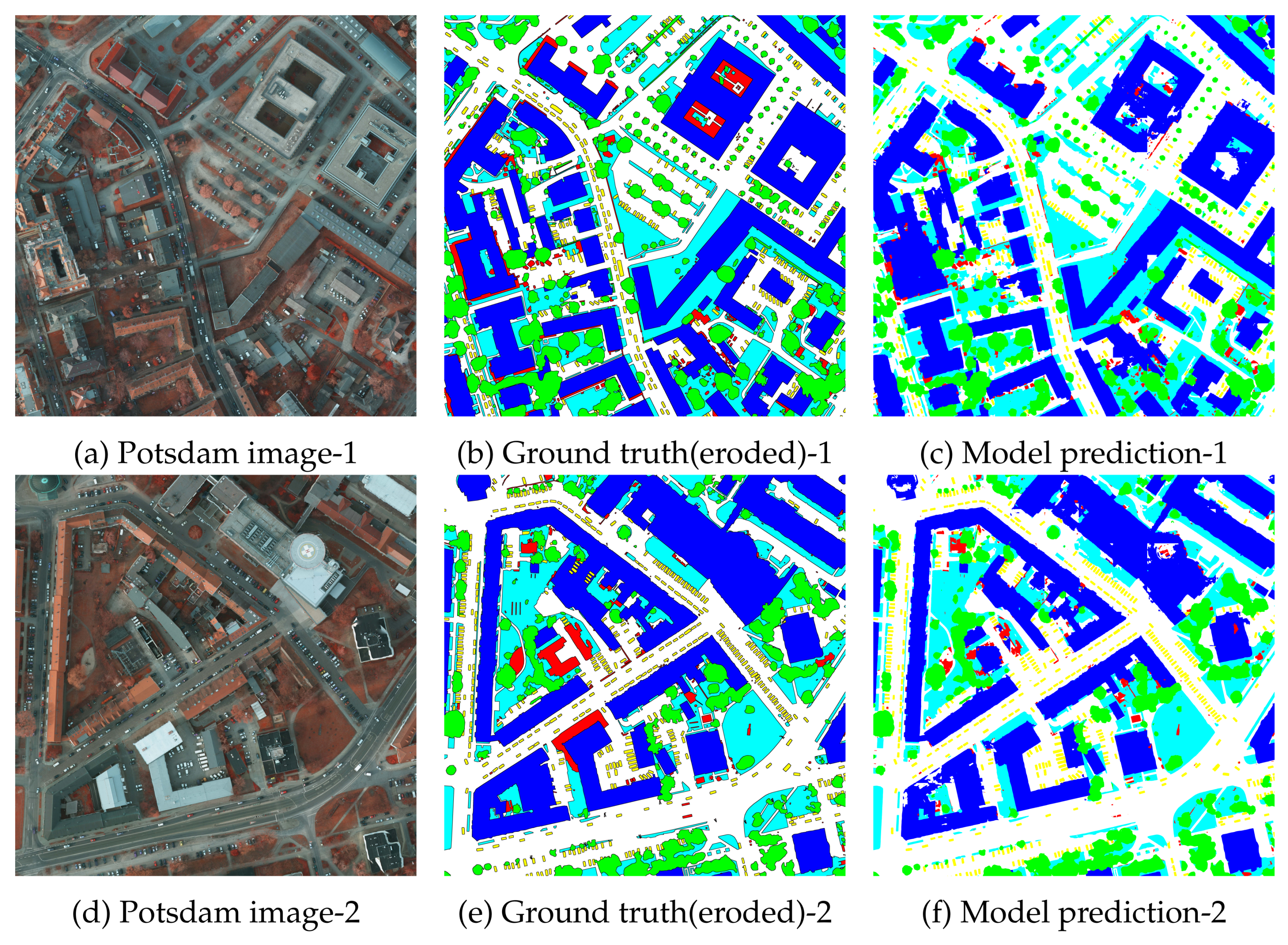
3.3.2. Potsdam Benchmark Evaluation
4. Discussion
4.1. Ablation Study
We decompose our network step-wise and validate the effect of each proposed module. This experiment is conducted on ISPRS Vaihingen local dataset. A ResNet-50 model is used as the base network, and the last feature map is directly upsampled as output. Firstly we evaluate the base model performance as Table 5 shows. Then following U-Net [30], we extend it to a similar encoder–decoder structure with Residual Convolutional Module only. This improves the performance from 69.3% to 75.9%. We then add proposed Context Fuse Module to exploit multi-scale features extensively. The performance increases from 75.9% to 76.5%. We further apply Attention Mix Module to fuse low-level and high-level features more adaptively, which gets another 0.3% improvement.
4.2. Model Performance
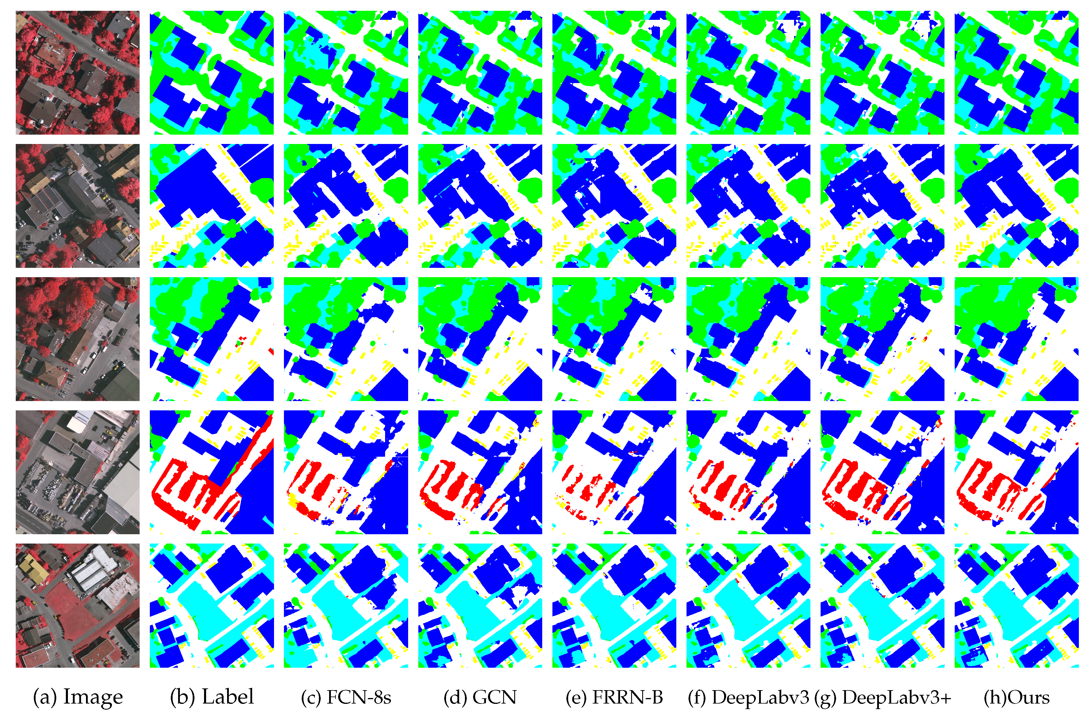
For local evaluation, other deep learning models cannot distinguish between background and other objects, including low vegetation, impervious surface, and building, as shown in Figure 6 and Figure 8. They often make mistakes when it comes to objects which are similar with background. Besides, for buildings with complex appearance, these models tend to classify parts of the building into wrong objects. For instance, buildings with “holes” and similar appearance to impervious surface are very likely to be misclassified. On the contrary, our CAN model shows better robustness to them. It can differentiate background from other objects much better than these deep learning models and achieve coherent labeling for confusing objects, even buildings with intricate appearance. Moreover, fine-structured objects can also be labeled with precise localization using our model.
For benchmark evaluation, our model outperforms other benchmark methods, as shown in Table 3 and Table 4. These methods not only utilizes image data, but also DSM/NDSM data, which would benefit building recognition a lot. Our model only takes use of raw image data without using DSM/NDSM data. Some methods consist of multi stages which are troublesome compared with our end-to-end method.
5. Conclusions
In this work, we introduce a novel end-to-end context aggregation network (CAN) for semantic labeling in aerial images. It has an encoder–decoder like architecture, with efficient context information aggregation and attention-based multi-level feature fusion. It consists of a Context Fuse Module (CFM), Attention Mix Module (AMM), and Residual Convolutional Module (RCM). CFM is composed of parallel convolutional layers with kernels of different sizes and a global pooling branch. Parallel convolutional layers aggregate context information with multiple receptive fields. The global pooling branch introduces global context information. AMM utilizes a channel-wise attention mechanism to combine multi-level features and selectively emphasizes more discriminative features. RCM refines features in all feature levels. With these modules, our network can combine multi-level features more efficiently, and exploits features more extensively.
We evaluate the proposed network on ISPRS Vaihingen and Potsdam datasets. Local evaluation results show our proposed CAN model also outperforms other state-of-the-art deep learning models on both datasets. Benchmark evaluation results show our proposed CAN model, which uses only raw image data, outperforms top methods on these datasets. Ablation study demonstrates the effectiveness of the proposed modules.
Author Contributions
W.C. designed the algorithm and performed the experiments; W.C. and W.Y. analyzed the data; W.C. wrote the paper; M.W., G.W. and J.C. revised the paper. All authors read and approved the submitted manuscript.
Funding
The research was partially supported by the National Natural Science Foundation of China (NSFC) under Grant 61771351, the CETC key laboratory of aerospace information applications under Grant SXX18629T022, and the project for innovative research groups of the natural science foundation of Hubei Province (No. 2018CFA006).
Acknowledgments
We thank the ISPRS for providing the research community with the awesome challenge datasets.
Conflicts of Interest
The authors declare no conflict of interest.
Abbreviations
The following abbreviations are used in this manuscript:
| CNNs | Convolutional Neural Networks |
| SIFT | Scale Invariant Feature Transform |
| HOG | Histogram of Oriented Gradients |
| FAST | Accelerated Segment Test |
| FCN | Fully Convolutional Networks |
| CFM | Context Fuse Module |
| AMM | Attention Mix Module |
| RCM | Residual Convolutional Module |
| CAN | Context Aggregation Network |
| IRRG | Infrared, Red and Green |
| DSM | Digital Surface Model |
| NDSM | Normalized Digital Surface Model |
| GSD | Ground Surface Distance |
| IRRGB | Infrared, Red, Green, Blue |
| SGD | Stochastic gradient descent |
| F1 | F1 score |
| OA | Overall Accuracy |
| IoU | Intersection over Union |
| PR | Precision-recall |
| CRF | Conditional Random Field |
References
- Li, J.; Huang, X.; Gamba, P.; Bioucas-Dias, J.M.; Zhang, L.; Benediktsson, J.A.; Plaza, A. Multiple feature learning for hyperspectral image classification. IEEE Trans. Geosci. Remote Sens. 2015, 53, 1592–1606. [Google Scholar] [CrossRef]
- Xue, Z.; Li, J.; Cheng, L.; Du, P. Spectralspatial classification of hyperspectral data via morphological component analysis-based image separation. IEEE Trans. Geosci. Remote Sens. 2015, 53, 70–84. [Google Scholar]
- Xu, X.; Li, J.; Huang, X.; Mura, M.D.; Plaza, A. Multiple morphological component analysis based decomposition for remote sensing image classification. IEEE Trans. Geosci. Remote Sens. 2016, 54, 3083–3102. [Google Scholar] [CrossRef]
- Moser, G.; Serpico, S.B.; Benediktsson, J.A. Land-cover mapping by Markov modeling of spatial-contextual information in very-high-resolution remote sensing images. Proc. IEEE 2013, 101, 631–651. [Google Scholar] [CrossRef]
- Lu, X.; Yuan, Y.; Zheng, X. Joint dictionary learning for multispectral change detection. IEEE Trans. Cybern. 2017, 47, 884–897. [Google Scholar] [CrossRef]
- Matikainen, L.; Karila, K. Segment-based land cover mapping of a suburban area-comparison of high-resolution remotely sensed datasets using classification trees and test field points. Remote Sens. 2011, 3, 1777–1804. [Google Scholar] [CrossRef]
- Zhang, Q.; Seto, K.C. Mapping urbanization dynamics at regional and global scales using multi-temporal dmsp/ols nighttime light data. Remote Sens. Environ. 2011, 115, 2320–2329. [Google Scholar] [CrossRef]
- Xin, P.; Jian, Z. High-resolution remote sensing image classification method based on convolutional neural network and restricted conditional random field. Remote Sens. 2018, 10, 920. [Google Scholar]
- Lowe, D.G. Distinctive image features from scale-invariant keypoints. Int. J. Comput. Vis. 2004, 60, 90–110. [Google Scholar] [CrossRef]
- Dalal, N.; Triggs, B. Histograms of oriented gradients for human detection. In Proceedings of the IEEE Conference on Vision and Pattern Recognition (CVPR), San Diego, CA, USA, 20–25 June 2005; pp. 886–893. [Google Scholar]
- Rosten, E.; Drummond, T. Machine learning for high-speed corner detection. In Proceedings of the European Conference on Computer Vision (ECCV), Graz, Austria, 7–13 May 2006; pp. 430–443. [Google Scholar]
- Turgay, C. Unsupervised change detection in satellite images using principal component analysis and k-means clustering. IEEE Geosci. Remote Sens. Lett. 2009, 3, 772–776. [Google Scholar] [CrossRef]
- Inglada, J. Automatic recognition of man-made objects in high resolution optical remote sending images by SVM classification of geometric image features. ISPRS J. Photogramm. Remote Sens. 2007, 62, 236–248. [Google Scholar] [CrossRef]
- Mariana, B.; Lucian, D. Random forest in remote sensing: A review of applications and future directions. ISPRS J. Photogramm. Remote Sens. 2016, 114, 24–31. [Google Scholar]
- Deng, J.; Dong, W.; Socher, R.; Li, L.J.; Li, K.; Li, F.-F. ImageNet: A large-scale hierarchical image database. In Proceedings of the IEEE International Conference on Computer Vision and Pattern Recognition (CVPR), Miami, FL, USA, 20–25 June 2009; pp. 248–255. [Google Scholar]
- Simonyan, K.; Zisserman, A. Very Deep Convolutional Networks for Large-Scale Image Recognition. arXiv, 2014; arXiv:1409.1556. [Google Scholar]
- He, K.; Zhang, X.; Ren, S.; Sun, J. Deep Residual Learning for Image Recognition. In Proceedings of the IEEE Conference on Computer Vision and Pattern Recognition (CVPR), Las Vegas, NV, USA, 26 June–1 July 2016; pp. 770–778. [Google Scholar]
- Huang, G.; Liu, Z.; Van Der Maaten, L.; Weinberger, K.Q. Densely connected convolutional networks. In Proceedings of the IEEE International Conference on Computer Vision and Pattern Recognition (CVPR), Honolulu, HI, USA, 21–26 July 2017; pp. 4700–4708. [Google Scholar]
- Mnih, V. Machine Learning for Aerial Image Labeling. Ph.D. Thesis, University of Toronto, Toronto, ON, Canada, 2013. [Google Scholar]
- Paisitkriangkrai, S.; Sherrah, J.; Janney, P.; van den Hengel, A. Semantic labeling of aerial and satellite imagery. IEEE J. Sel. Top. Appl. Earth Obs. 2016, 9, 2868–2881. [Google Scholar] [CrossRef]
- Nogueira, K.; Mura, M.D.; Chanussot, J.; Schwartz, W.R.; Santos, J.A.D. Learning to semantically segment highresolution remote sensing images. Proceedings of IEEE International Conference on Pattern Recognition (ICPR), Cancun, Mexico, 4–8 December 2016; pp. 3566–3571. [Google Scholar]
- Alshehhi, R.; Marpu, P.R.; Woon, W.L.; Mura, M.D. Simultaneous extraction of roads and buildings in remote sensing imagery with convolutional neural networks. ISPRS J. Photogramm. Remote Sens. 2017, 130, 139–149. [Google Scholar] [CrossRef]
- Zhang, C.; Pan, X.; Li, H.; Gardiner, A.; Sargent, I.; Hare, J.; Atkinson, P.M. A hybrid MLP-CNN classifier for very fine resolution remotely sensed image classification. ISPRS J. Photogramm. Remote Sens. 2018, 140, 133–144. [Google Scholar] [CrossRef]
- Maggiori, E.; Tarabalka, Y.; Charpiat, G.; Alliez, P. Convolutional neural networks for large-scale remote-sensing image classification. IEEE Trans. Geosci. Remote Sens. 2017, 55, 645–657. [Google Scholar] [CrossRef]
- Mostajabi, M.; Yadollahpour, P.; Shakhnarovich, G. Feedforward semantic segmentation with zoom-out features. In Proceedings of the IEEE International Conference on Computer Vision and Pattern Recognition (CVPR), Boston, MA, USA, 8–10 June 2015; pp. 3376–3385. [Google Scholar]
- Zhao, W.; Jiao, L.; Ma, W.; Zhao, J.; Zhao, J.; Liu, H.; Cao, X.; Yang, S. Superpixel-based multiple local cnn for panchromatic and multispectral image classification. IEEE Trans. Geosci. Remote Sens. 2017, 55, 4141–4156. [Google Scholar] [CrossRef]
- Long, J.; Shelhamer, E.; Darrell, T. Fully convolutional networks for semantic segmentation. In Proceedings of the IEEE International Conference on Computer Vision and Pattern Recognition (CVPR), Boston, MA, USA, 8–10 June 2015; pp. 3431–3440. [Google Scholar]
- Noh, H.; Hong, S.; Han, B. Learning deconvolution network for semantic segmentation. In Proceedings of the IEEE International Conference on Computer Vision (ICCV), Santiago, Chile, 11–18 December 2015; pp. 1520–1528. [Google Scholar]
- Badrinarayanan, V.; Kendall, A.; Cipolla, R. Segnet: A deep convolutional encoder-decoder architecture for image segmentation. IEEE Trans. Pattern Anal. Mach. Intell. 2017, 39, 2481–2495. [Google Scholar] [CrossRef] [PubMed]
- Ronneberger, O.; Fischer, P.; Brox, T. U-net: Convolutional networks for biomedical image segmentation. In Proceedings of the International Conference on Medical Image Computing and Computer Assisted Intervention(MICCAI), Munich, Germany, 5–9 October 2015; pp. 234–241. [Google Scholar]
- Pohlen, T.; Hermans, A.; Mathias, M.; Leibe, B. Full-resolution residual networks for semantic segmentation in street scenes. In Proceedings of the IEEE International Conference on Computer Vision and Pattern Recognition (CVPR), Honolulu, HI, USA, 21–26 July 2017; pp. 4151–4160. [Google Scholar]
- Lin, G.; Milan, A.; Shen, C.; Reid, I. Refinenet: Multi-path refinement networks for high-resolution semantic segmentation. In Proceedings of the IEEE International Conference on Computer Vision and Pattern Recognition (CVPR), Honolulu, HI, USA, 21–26 July 2017; pp. 1925–1934. [Google Scholar]
- Zhao, H.; Shi, J.; Qi, X.; Wang, X.; Jia, J. Pyramid scene parsing network. In Proceedings of the IEEE International Conference on Computer Vision and Pattern Recognition (CVPR), Honolulu, HI, USA, 21–26 July 2017; pp. 2881–2890. [Google Scholar]
- Chen, L.; Papandreou, G.; Kokkinos, I.; Murphy, K.P.; Yuille, A.L. Semantic Image Segmentation with Deep Convolutional Nets and Fully Connected CRFs. In Proceedings of the International Conference on Learning Representations (ICLR), San Diego, CA, USA, 7–9 May 2015; pp. 5168–5177. [Google Scholar]
- Chen, L.C.; Papandreou, G.; Schroff, F.; Adam, H. Rethinking atrous convolution for semantic image segmentation. arXiv, 2017; arXiv:1706.05587. [Google Scholar]
- Peng, C.; Zhang, X.; Yu, G.; Luo, G.; Sun, J. Large Kernel Matters–Improve Semantic Segmentation by Global Convolutional Network. In Proceedings of the IEEE International Conference on Computer Vision and Pattern Recognition (CVPR), Honolulu, HI, USA, 21–26 July 2017; pp. 4353–4361. [Google Scholar]
- Zhang, H.; Dana, K.; Shi, J.; Zhang, Z.; Wang, X.; Tyagi, A.; Agrawal, A. Context encoding for semantic segmentation. In Proceedings of the IEEE Conference on Computer Vision and Pattern Recognition (CVPR), Salt Lake City, UT, USA, 18–22 June 2018; pp. 7151–7160. [Google Scholar]
- Yu, F.; Koltun, V. Multi-scale context aggregation by dilated convolutions. In Proceedings of the International Conference on Learning Representations (ICLR), Caribe Hilton, San Juan, Puerto Rico, 2–4 May 2016. [Google Scholar]
- Wang, P.; Chen, P.; Yuan, Y.; Liu, D.; Huang, Z.; Hou, X.; Cottrell, G. Understanding convolution for semantic segmentation. In Proceedings of the IEEE Winter Conference on Applications of Computer Vision(WACV), Lake Tahoe, NV, USA, 12–15 March 2018; pp. 1451–1460. [Google Scholar]
- Ioffe, S.; Szegedy, C. Batch Normalization: Accelerating Deep Network Training by Reducing Internal Covariate Shift. Proceedings of International Conference on Machine Learning(ICML), San Diego, CA, USA, 7–9 May 2015; pp. 448–456. [Google Scholar]
- Krizhevsky, A.; Sutskever, I.; Hinton, G.E. Imagenet classification with deep convolutional neural networks. In Proceedings of the International Conference on Neural Information Processing Systems (NeurIPS), Lake Tahoe, NV, USA, 3–6 December 2012; pp. 1097–1105. [Google Scholar]
- Liu, W.; Rabinovich, A.; Berg, A.C. Parsenet: Looking wider to see better. In Proceedings of the International Conference on Learning Representations (ICLR), Caribe Hilton, San Juan, Puerto Rico, 2–4 May 2016. [Google Scholar]
- Chen, L.C.; Zhu, Y.; Papandreou, G.; Schroff, F.; Adam, H. Encoder-decoder with atrous separable convolution for semantic image segmentation. In Proceedings of the European Conference on Computer Vision (ECCV), Munich, Germany, 8–14 September 2018; pp. 801–818. [Google Scholar]
- Hu, J.; Shen, L.; Sun, G. Squeeze-and-excitation networks. In Proceedings of the IEEE Conference on Computer Vision and Pattern Recognition (CVPR), Salt Lake City, UT, USA, 18–22 June 2018; pp. 7132–7141. [Google Scholar]
- Yu, C.; Wang, J.; Peng, C.; Gao, C.; Yu, G.; Sang, N. Learning a discriminative feature network for semantic segmentation. In Proceedings of the IEEE Conference on Computer Vision and Pattern Recognition (CVPR), Salt Lake City, UT, USA, 18–22 June 2018; pp. 1857–1866. [Google Scholar]
- ISPRS. International Society For Photogrammetry And Remote Sensing. 2D Semantic Labeling Challenge. 2016. Available online: http://www2.isprs.org/commissions/comm3/wg4/semantic-labeling.html (accessed on 13 May 2019).
- Piramanayagam, S.; Saber, E.; Schwartzkopf, W.; Koehler, F. Supervised Classification of Multisensor Remotely Sensed Images Using a Deep Learning Framework. Remote Sens. 2018, 10, 1429. [Google Scholar] [CrossRef]
- Liu, Y.; Fan, B.; Wang, L.; Bai, J.; Xiang, S.; Pan, C. Context-aware cascade network for semantic labeling in VHR image. In Proceedings of the IEEE International Conference on Image Processing (ICIP), Beijing, China, 17–20 September 2017; pp. 575–579. [Google Scholar]
- Gerke, M. Use of the Stair Vision Library within the ISPRS 2d Semantic Labeling Benchmark (Vaihingen); Technical Report; University of Twente: Enschede, The Netherlands, 2015. [Google Scholar]
- Gould, S.; Russakovsky, O.; Goodfellow, I.; Baumstarck, P. The Stair Vision Library (v2.5); Stanford University: Stanford, CA, USA, 2011. [Google Scholar]
- Volpi, M.; Tuia, D. Dense semantic labeling of subdecimeter resolution images with convolutional neural networks. IEEE Trans. Geosci. Remote Sens. 2017, 55, 881–893. [Google Scholar] [CrossRef]
- Sherrah, J. Fully convolutional networks for dense semantic labelling of high-resolution aerial imagery. arXiv, 2016; arXiv:1606.02585. [Google Scholar]
- Marmanis, D.; Schindler, K.; Wegner, J.D.; Galliani, S.; Datcu, M.; Stilla, U. Classification with an edge: Improving semantic image segmentation with boundary detection. ISPRS J. Photogramm. Remote Sens. 2018, 135, 158–172. [Google Scholar] [CrossRef] [Green Version]
- Kemker, R.; Salvaggio, C.; Kanan, C. Algorithms for semantic segmentation of multispectral remote sensing imagery using deep learning. ISPRS J. Photogramm. Remote Sens. 2018, 145, 60–77. [Google Scholar] [CrossRef] [Green Version]
Figure 1.
An overview of our proposed Context Aggregation Network. Red lines represent bilinear upsample operation. CFM: Context Fuse Module, AMM: Attention Mix Module, RCM: Residual Convolutional Module.
Figure 1.
An overview of our proposed Context Aggregation Network. Red lines represent bilinear upsample operation. CFM: Context Fuse Module, AMM: Attention Mix Module, RCM: Residual Convolutional Module.

Figure 2.
Context Fuse Module structure. Part A is a parallel convolutional block. Part B is a global pooling branch. Red line represents bilinear upsample operation.
Figure 2.
Context Fuse Module structure. Part A is a parallel convolutional block. Part B is a global pooling branch. Red line represents bilinear upsample operation.

Figure 3.
Attention Mix Module structure. Red line represents bilinear upsample operation.

Figure 4.
Residual Convolutional Module structure.

Figure 5.
Samples of ISPRS Vaihingen dtaset and Potsdam dataset. There are 5 labeled categories and background (white: impervious surface, blue: building, cyan: low vegetation, green: tree, yellow: car, red: clutter/background).
Figure 5.
Samples of ISPRS Vaihingen dtaset and Potsdam dataset. There are 5 labeled categories and background (white: impervious surface, blue: building, cyan: low vegetation, green: tree, yellow: car, red: clutter/background).

Figure 6.
Visual comparisons with deep learning models of local evaluation on ISPRS Vaihingen dataset (white: impervious surface, blue: building roof, cyan: low vegetation, green: tree, yellow: car, red: clutter/background).
Figure 6.
Visual comparisons with deep learning models of local evaluation on ISPRS Vaihingen dataset (white: impervious surface, blue: building roof, cyan: low vegetation, green: tree, yellow: car, red: clutter/background).

Figure 7.
Precision-recall (PR) curves of all the comparing deep learning models on Vaihingen local evaluation. Categories from left to right: impervious surface (imp surf), building, low vegetation (low veg), tree, car.
Figure 7.
Precision-recall (PR) curves of all the comparing deep learning models on Vaihingen local evaluation. Categories from left to right: impervious surface (imp surf), building, low vegetation (low veg), tree, car.

Figure 8.
Visual comparisons with deep learning models of local evaluation on ISPRS Potsdam dataset (white: impervious surface, blue: building roof, cyan: low vegetation, green: tree, yellow: car, red: clutter/background).
Figure 8.
Visual comparisons with deep learning models of local evaluation on ISPRS Potsdam dataset (white: impervious surface, blue: building roof, cyan: low vegetation, green: tree, yellow: car, red: clutter/background).

Figure 9.
Precision-recall (PR) curves of all the comparing deep learning models on Potsdam local evaluation. Categories from left to right: impervious surface (imp surf), building, low vegetation (low veg), tree, car.
Figure 9.
Precision-recall (PR) curves of all the comparing deep learning models on Potsdam local evaluation. Categories from left to right: impervious surface (imp surf), building, low vegetation (low veg), tree, car.

Figure 10.
Visual results of benchamark evaluation on ISPRS Vaihingen dataset.

Figure 11.
Visual results of benchamark evaluation on the ISPRS Potsdam dataset.


Table 1.
Local evaluation results on ISPRS Vaihingen dataset. Imp surf: impevious surfaces. Low veg: low vegetation. MIoU: average of five objects’ IoUs. MF1: acerage of five obejects’ F1 scores. Acc.: overall accuracy.
Table 1.
Local evaluation results on ISPRS Vaihingen dataset. Imp surf: impevious surfaces. Low veg: low vegetation. MIoU: average of five objects’ IoUs. MF1: acerage of five obejects’ F1 scores. Acc.: overall accuracy.
| Model | Imp surf | Building | Low veg | Tree | Car | Avg. | |||||||
|---|---|---|---|---|---|---|---|---|---|---|---|---|---|
| IoU | F1 | IoU | F1 | IoU | F1 | IoU | F1 | IoU | F1 | mIoU | mF1 | Acc. | |
| FCN-8s [27] | 80.3 | 89.1 | 83.0 | 90.7 | 67.4 | 80.6 | 73.4 | 84.7 | 58.3 | 73.7 | 72.5 | 83.7 | 85.9 |
| GCN [36] | 81.6 | 89.8 | 86.2 | 92.6 | 68.5 | 81.3 | 74.2 | 85.2 | 61.4 | 76.1 | 74.4 | 85.0 | 86.9 |
| FRRN-B [31] | 81.5 | 89.8 | 86.8 | 92.9 | 68.5 | 81.3 | 73.6 | 84.8 | 63.6 | 77.7 | 74.8 | 85.3 | 86.9 |
| DeepLabv3 [35] | 81.8 | 90.0 | 87.4 | 93.3 | 70.0 | 82.3 | 74.5 | 85.4 | 61.2 | 75.9 | 75.0 | 85.4 | 87.4 |
| DeepLabv3+ [43] | 81.2 | 89.6 | 86.7 | 92.9 | 68.6 | 81.4 | 74.9 | 85.6 | 64.3 | 78.3 | 75.1 | 85.5 | 87.2 |
| Ours | 82.6 | 90.5 | 87.2 | 93.1 | 70.3 | 82.5 | 75.2 | 85.9 | 68.7 | 81.4 | 76.8 | 86.7 | 87.8 |
Table 2.
Local evaluation results on ISPRS Potsdam dataset. Imp surf: impevious surfaces. Low veg: low vegetation. MIoU: average of five objects’ IoUs. MF1: acerage of five obejects’ F1 scores. Acc.: overall accuracy.
Table 2.
Local evaluation results on ISPRS Potsdam dataset. Imp surf: impevious surfaces. Low veg: low vegetation. MIoU: average of five objects’ IoUs. MF1: acerage of five obejects’ F1 scores. Acc.: overall accuracy.
| Model | Imp surf | Building | Low veg | Tree | Car | Avg. | |||||||
|---|---|---|---|---|---|---|---|---|---|---|---|---|---|
| IoU | F1 | IoU | F1 | IoU | F1 | IoU | F1 | IoU | F1 | mIoU | mF1 | Acc. | |
| FRRN-B [31] | 78.6 | 88.0 | 86.2 | 92.6 | 68.9 | 81.6 | 70.1 | 82.4 | 78.1 | 87.7 | 76.4 | 86.5 | 85.5 |
| FCN-8s [27] | 79.6 | 88.6 | 86.0 | 92.4 | 70.1 | 82.4 | 70.8 | 82.9 | 78.3 | 87.8 | 77.0 | 86.8 | 86.1 |
| GCN [36] | 80.1 | 88.9 | 87.5 | 93.3 | 70.1 | 82.4 | 70.7 | 82.8 | 78.1 | 87.7 | 77.3 | 87.0 | 86.4 |
| DeepLabv3 [35] | 80.7 | 89.3 | 88.5 | 93.9 | 69.9 | 82.3 | 70.4 | 82.6 | 78.7 | 88.1 | 77.7 | 87.2 | 86.7 |
| DeepLabv3+ [43] | 80.6 | 89.2 | 88.5 | 93.9 | 70.3 | 82.6 | 71.2 | 83.2 | 80.1 | 88.9 | 78.1 | 87.6 | 86.5 |
| Ours | 80.7 | 89.3 | 86.8 | 92.9 | 71.0 | 83.0 | 72.7 | 84.2 | 79.6 | 88.6 | 78.2 | 87.6 | 86.9 |
Table 3.
Benchmark evluation results on the ISPRS Vaihingen dataset (class F1 score and overall accuracy). Imp surf: impevious surfaces. Low veg: low vegetation.
Table 3.
Benchmark evluation results on the ISPRS Vaihingen dataset (class F1 score and overall accuracy). Imp surf: impevious surfaces. Low veg: low vegetation.
| Methods | Imp surf | Building | Low veg | Tree | Car | Overall Acc.(%) |
|---|---|---|---|---|---|---|
| SVL_6 [49] | 86.0 | 90.2 | 75.6 | 82.1 | 45.4 | 83.2 |
| UZ_1 [51] | 89.2 | 92.5 | 81.6 | 86.9 | 57.3 | 87.3 |
| ADL_3 [20] | 89.5 | 93.2 | 82.3 | 88.2 | 63.3 | 88.0 |
| DST_2 [52] | 90.5 | 93.7 | 83.4 | 89.2 | 72.6 | 89.1 |
| DLR_8 [53] | 90.4 | 93.6 | 83.9 | 89.7 | 76.9 | 89.2 |
| CASIA [48] | 92.7 | 95.3 | 84.3 | 89.6 | 80.8 | 90.6 |
| Ours | 93.0 | 95.8 | 85.0 | 90.2 | 89.7 | 91.2 |
Table 4.
Benchmark evluation results on ISPRS Potsdam dataset (class F1 score and overall accuracy). Imp surf: impevious surfaces. Low veg: low vegetation.
Table 4.
Benchmark evluation results on ISPRS Potsdam dataset (class F1 score and overall accuracy). Imp surf: impevious surfaces. Low veg: low vegetation.
| Methods | Imp surf | Building | Low veg | Tree | Car | Overall Acc.(%) |
|---|---|---|---|---|---|---|
| SVL_3 [49] | 84.0 | 89.8 | 72.0 | 59.0 | 69.8 | 77.2 |
| UZ_1 [51] | 89.3 | 95.4 | 81.8 | 80.5 | 86.5 | 85.8 |
| KLab_2 [54] | 89.7 | 92.7 | 83.7 | 84.0 | 92.1 | 86.7 |
| RIT_2 [47] | 92.0 | 96.3 | 85.5 | 86.5 | 94.5 | 89.4 |
| DST_2 [52] | 91.8 | 95.9 | 86.3 | 87.7 | 89.2 | 89.7 |
| Ours | 93.1 | 96.4 | 87.7 | 88.8 | 95.9 | 90.9 |
Table 5.
Detailed performance comparison of network modules (class IoU and mean IoU). RCM: Residual Convolutional Module. CFM: Context Fuse Module. AMM: Attention Mix Module.
Table 5.
Detailed performance comparison of network modules (class IoU and mean IoU). RCM: Residual Convolutional Module. CFM: Context Fuse Module. AMM: Attention Mix Module.
| Model | Imp surf | Building | Low veg | Tree | Car | Mean IoU(%) |
|---|---|---|---|---|---|---|
| Res-50 | 78.2 | 85.4 | 66.9 | 72.8 | 43.5 | 69.3 |
| Res-50+RCM | 81.9 | 87.1 | 69.8 | 75.2 | 65.6 | 75.9 |
| Res-50+RCM+CFM | 82.2 | 87.3 | 70.1 | 75.6 | 67.1 | 76.5 |
| Res-50+RCM+CFM+AMM | 82.6 | 87.2 | 70.3 | 75.2 | 68.7 | 76.8 |
© 2019 by the authors. Licensee MDPI, Basel, Switzerland. This article is an open access article distributed under the terms and conditions of the Creative Commons Attribution (CC BY) license (http://creativecommons.org/licenses/by/4.0/).
Share and Cite
MDPI and ACS Style
Cheng, W.; Yang, W.; Wang, M.; Wang, G.; Chen, J. Context Aggregation Network for Semantic Labeling in Aerial Images. Remote Sens. 2019, 11, 1158. https://0-doi-org.brum.beds.ac.uk/10.3390/rs11101158
AMA Style
Cheng W, Yang W, Wang M, Wang G, Chen J. Context Aggregation Network for Semantic Labeling in Aerial Images. Remote Sensing. 2019; 11(10):1158. https://0-doi-org.brum.beds.ac.uk/10.3390/rs11101158
Chicago/Turabian StyleCheng, Wensheng, Wen Yang, Min Wang, Gang Wang, and Jinyong Chen. 2019. "Context Aggregation Network for Semantic Labeling in Aerial Images" Remote Sensing 11, no. 10: 1158. https://0-doi-org.brum.beds.ac.uk/10.3390/rs11101158
Note that from the first issue of 2016, this journal uses article numbers instead of page numbers. See further details here.