1. Introduction
Obtaining the fine structure and the characteristics of the ionosphere during both quiet and active ionospheric periods and during magnetic storms is one of the focal points of space science research [
1,
2]. In recent years, an increasing number of scholars have postulated that more accurate results can be obtained by monitoring ionospheric activities and evaluating ionospheric irregularities through Kalman updates and by analyzing the time evolution of theoretical and empirical models. The use of multisource data, especially ground-based/spaceborne observation data, could greatly enrich the available information regarding horizontal and vertical ionospheric structures.
At present, obtaining a more accurate description of the ionosphere is achieved mainly in three ways. (1) The physical ionosphere model, such as SAMI3 [
3], and the National Center for Atmospheric Research (NCAR) thermosphere–ionosphere–electrodynamics general circulation model (TIE-GCM) [
4] are improved by coupling its physical mechanism with the thermal layer or the plasmasphere. (2) Ionospheric climate models are established through measured data, examples of which include NeQuick [
5], the international reference ionosphere (IRI) model [
6], the Global Core Plasma Model (GCPM) [
7], IRI_Plas [
8,
9] and the model developed by Wu [
10,
11,
12], which improves the IRI model with Constellation Observing System for Meteorology, Ionosphere, and Climate (COSMIC) occultation data. (3) Based on either a function basis or a pixel basis, various methods, including the Kalman filter, three/four-dimensional variational data assimilation (3D-var/4D-var), and Optimal Interpolation (I/O), have been used to assimilate physical models or climate models to obtain a precise and accurate ionospheric structure [
13,
14,
15,
16,
17]. Based on the above-mentioned studies, this study sought to model the ionosphere by using observation data to update the climate model by applying Kalman filtering, which not only employs grid division based on the vertical structure of the ionospheric electron density (
Section 3.2), but also introduces the influences of differential code biases (DCBs) within receivers and transmitters (
Section 2.2).
Numerous contributions have been reported to obtain the fine structure of the ionosphere. However, as described by Fu et al. [
18], the errors caused by ionospheric assimilation algorithms are smaller than those corresponding to the plasmasphere with altitude above 800 km (in this paper, the altitudes 800 km and above are collectively called the top region, and those below 800 km are called the bottom region). Considering the storage space and the amount and accuracy of required calculations, C. H. Chen set the ionospheric assimilation height to 3000 km and excluded the contributions of higher components from ground-based ionospheric observation data by extending the top of the IRI model using an exponential decay function [
19]. Ercha Aa gave a clear view of three-dimentional electron density distribution over china using three-dimensional variational approach to handle the computational cost with a similar approach [
20]. L. C. Gardner applied the podTec observation data assimilated in the range of 80–3000 km of the ionosphere, but it was difficult to avoid the uneven distribution of information between the top region and bottom region [
21].
Many researchers have proposed different methods to obtain the ionospheric structure from a variety of perspectives [
10,
22,
23,
24,
25] using multisource data, as shown in
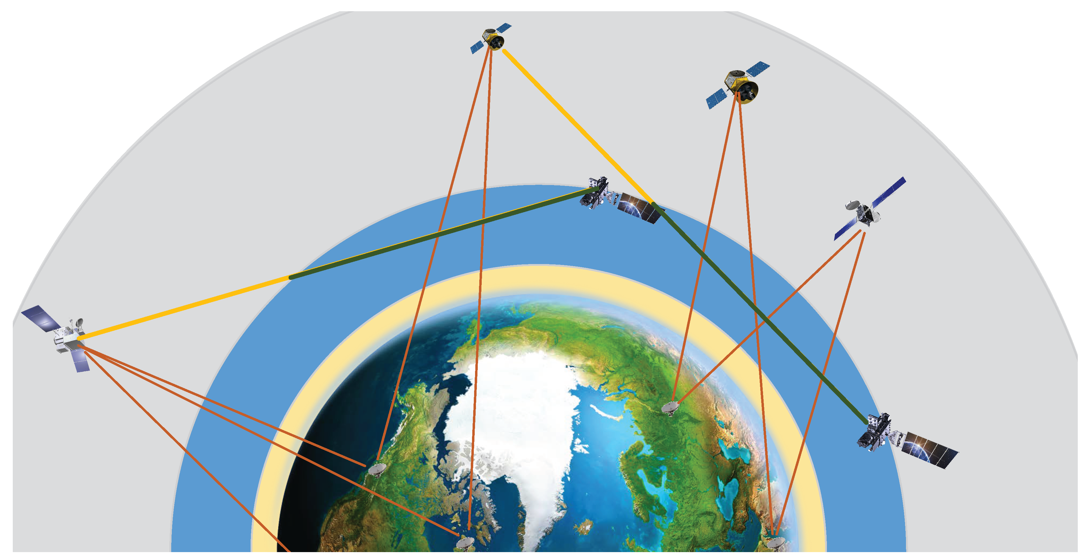
Figure 1, especially COSMIC podTec data and occultation data for spaceborne observations which avoid satellite and land distribution problems and cover the full range of the ionosphere. In the assimilation or computational ionospheric tomography (CIT) process, these techniques use the STECs obtained from the level-1 ionospheric product (ionPhs) along with ground-based observation as observation data [
26]. Conversely, these techniques use the STECs obtained from the level-1 ionospheric product (podTEC) as observation data to construct the ionosphere of the top region [
10,
25].
Although the methods above integrate various observation data into the ionospheric model in different ways, the uneven distribution of information between the top region and bottom region and the discontinuities between the top and bottom regions still exist. To ameliorate this problem, Wu did many works. Firstly, Wu reconstructed the F-layer ionospheric parameters by the spherical harmonic function using COSMIC ionPrf data, greatly improving the accuracy of the IRI model [
11]. Secondly, to construct the ionospheric structure of the top region, occultation data (ionPrf) were used for the top region to obtain a more accurate base for the electron density decay function with the altitude, and the electron density decay coefficients are the scale height of the top region obtained from vertical TECs mapped from podTEC data, which drops the horizontal structure information in podTec data [
12].
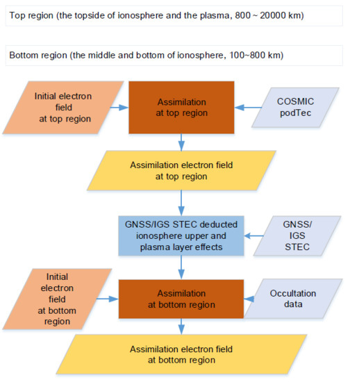
Based on Wu et al.’s research, a two-part step-by-step assimilation algorithm at the top/bottom region that considers the DCBs’ error of the instruments was used to solve the problem caused by inconsistencies in the ionospheric range. Firstly, the horizontal structure information in podTec was assimilated in the model of the top region introduced by We et al. Then, the horizontal structure information in the occultation observation data was utilized with ground-based GNSS ionospheric observations in the ionospheric assimilation model for the bottom region to obtain the ionospheric structure of the F2 layer. At the same time, geomagnetic corrections for ionospheric time variations were introduced to reduce the errors caused by changes in the ionosphere within the assimilation time window. Furthermore, we validated and discussed the effects of this correction on the error of the hypothesized model in the ionospheric assimilation with the global ionospheric model (GIM) from the International Global Navigation Satellite Systems (GNSS) Service (IGS).
The improved Kalman filtering assimilation algorithm used in this study is described in
Section 2. The data sources, processing methods and data sampling procedure in the two-part step-by-step assimilation technique are introduced in
Section 3. GIMs from different institutions, ionosonde data, incoherent scatter radar (ISR) data, and the electron density profile (EDP) from ionPrf in the COSMIC Data Analysis and Archive Center (CDAAC)/University Corporation for Atmospheric Research (UCAR) are used in
Section 4 to verify and evaluate the assimilation results. Finally, the effects of the hypothesized ionospheric errors in the measured observations and the sensitivities of different models to occultation data are discussed in
Section 5.
2. Methods
The classic Kalman filtering process includes two processes: a time evaluation and a status update. Since the covariance matrix is excessively large and a non-closed ionospheric system causes a substantial error in the theoretical model, the time evaluation step in the general assimilation process was discarded, and the predicted state of the theoretical or empirical model was used as the background. The field was incrementally updated only by the Kalman filtering update equation in the form of 3D-Var with the first guess at appropriate time (3D-FGAT). This article was also based on the above assumptions; accordingly, the main Kalman filtering equation for ionospheric assimilation can be derived as follows:
or can be transformed to the following:
where
K is the Kalman gain matrix in this epoch;
H is the observation matrix;
is the weight of the initial model;
Y is observation value such as STECs or electron densities;
and
are the prior and assimilated electron densities, respectively;
and
are the error covariances of the background model and observations, respectively; and
w is a temporary variable. In general, the background field is updated by Equation (
2) to avoid matrix inversion. However, the above formula does not consider the impacts of the DCBs of geostationary (GEO) satellites, low-Earth orbit (LEO) satellites and stations on the assimilation process.
2.1. Model of Observation Errors
According to the positional relationship among GEO/LEO and stations, ionospheric observation data can be divided into horizontal observations and vertical observations by the vertical angular distribution, and the weight of each observation can be determined by:
where
O is the weight of each observation type.
represents the observation data, slant total electron contents (STEC).
are the fixed error and the scale error, respectively.
constitute
as the weight of each observation.
The covariance matrix of the background model was determined by a Gaussian distribution:
therefore,
where
x represents
denoting the latitude, longitude, and altitude in succession and
is the error rate of the background model.
2.2. Introducing the DCBs of Receivers and Transmitters
The Center for Orbit Determination in Europe (CODE) and other research institutes obtain the solution DCB based on the single-layer ionospheric hypothesis; however, the top region of the ionosphere is affected by magnetic storms and possesses a complex spatial environment. The resulting errors are transmitted mainly to the absolute slant total electron content (STEC). The root mean square (RMS) DCBs of GNSS stations solved by the CODE/IGS institutions and the DCBs of the GPS/LEO observations in the podTec data from COSMIC used to estimate the errors of the DCBs were added to the background field of the ionosphere to obtain the STEC error. Accordingly, the STEC error was suppressed during assimilation.
The following observational equation was employed for additional electron density observations:
where
is the projection matrix obtained by ray tracing for ground-based/spaceborne observations;
and
are the DCB coefficients of the transmitters and receivers;
is the coefficient of the
jth grid for the
kth electron density observation data point;
is the electron density of the
j grid;
are the assimilated DCB differences between the DCBs of the transmitters and receivers and the CODE transmitter and receiver DCBs, respectively; and
are the observed STEC values obtained through the CODE/IGS products and the electron densities, respectively.
The model error can be written as:
The DCBs error was determined by the RMS of the IGS/CODE DCB product:
where
are the DCB errors of transmitters and receivers, respectively;
C is speed of light;
are the DCB RMSs of transmitters and receivers from CODE DCB product, respectively.
If electron density observation data were introduced during the assimilation process, then:
where
is the error of electron density observation data, and
is a fixed value representing the electron density error.
Finally, we can obtain the ionospheric update equation considering the effects of DCBs:
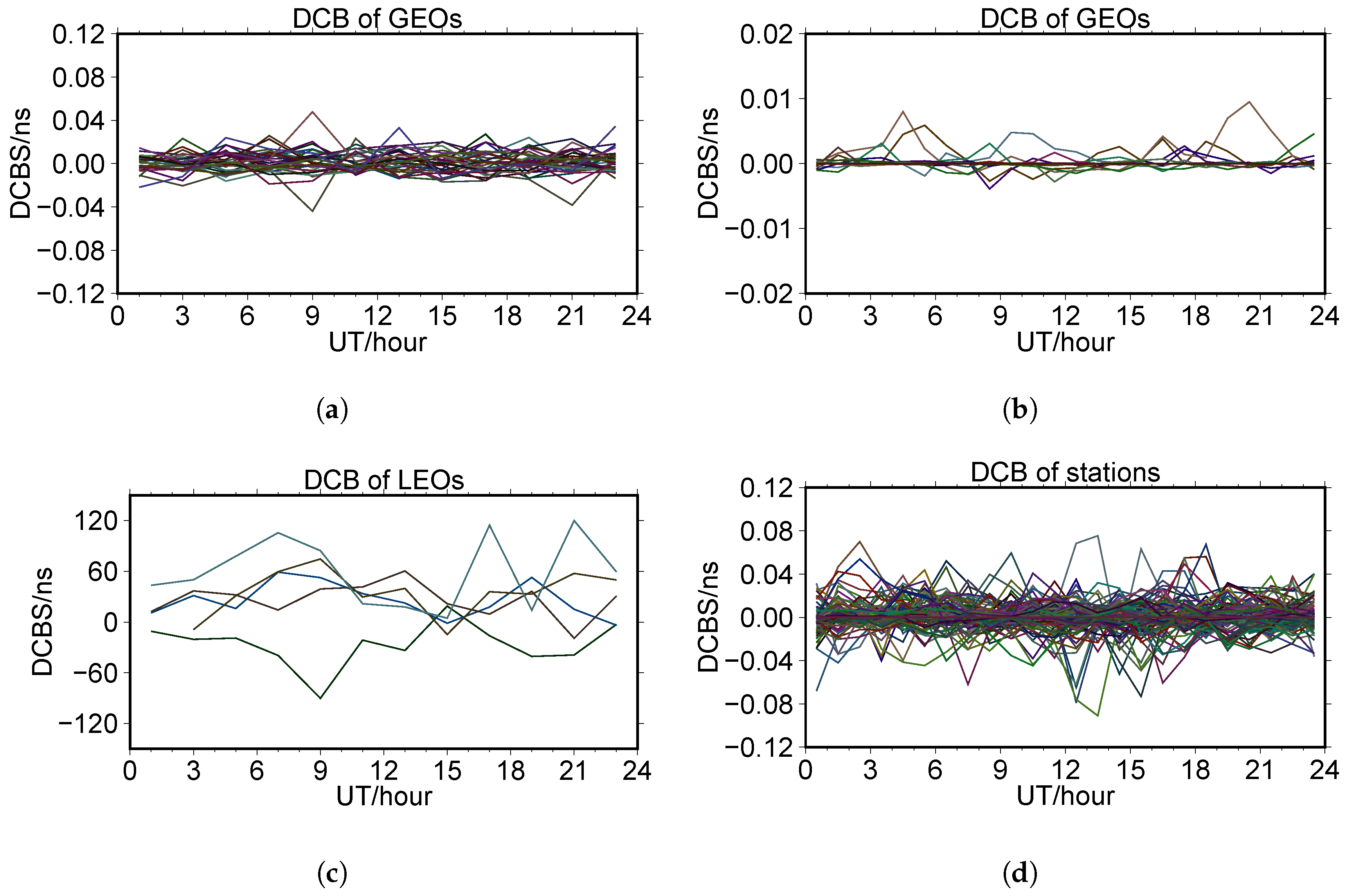
Figure 2 shows the corrected CODE DCBs obtained on DOY 010, 2008. Since the RMS DCBs, which contained very large errors (different data center errors can reach 2–6 TEC units (TECU); the LEO DCB solution error is 0.5 ns), were used to evaluate the assimilation accuracy, the RMS DCBs can be used only as the data weight for each station. The following is a brief analysis of the changes in the DCB weights for the assimilation of the top and bottom regions of the ionosphere.
The data for the top region can be referenced by using the podTec data from COSMIC. On DOY 10, 2008, the observations were concentrated mainly at 2–10 TECU, the RMS DCBs of the GPS observations were approximately 0.023 ns, and the LEO RMS DCB reached 0.5 ns or even 0.765 ns. At the same time, Lin found that DCB errors of COSMIC satellites showed a parabolic change with the elevation angle in the DCB estimation for GPS/LEO. When the elevation angle was
, the DCB errors of COSMIC satellites reached the lowest value with 0.24 TECU, and the errors at elevation angles of and were 0.4 TECU and 0.56 TECU, respectively [
27]. In the assimilation process, the fixed error and the proportional error of the observation error were 0.5 TECU and 0.12, respectively, and the specific weighted DCB error reached or exceeded the background field model error, indicating that the podTec error was absorbed by the DCB of GPS/LEO during the assimilation of the top ionospheric region. Therefore, the DCB correction of GPS/LEO could be 30–40 ns or even more than 80 ns in
Figure 2c.
For the assimilation of the bottom region, on DOY 10, 2008, the ground-based GNSS STEC observation was generally distributed at 30–100 TECU, and the RMS DCB of each station was generally within 0.1 ns. The fixed error and the proportional error of the observation error during the assimilation process were 0.5 TECU and 0.15, respectively. Therefore, the DCB error proportion was extremely low compared with the background field and observation data errors; however, if the RMS DCB of a station was extremely large, the observation data of that station can be suppressed.
Figure 2b,d demonstrate that the DCB corrections for the satellites and stations during the assimilation process were extremely small (all below 0.5 ns), which is consistent with the stability of DANGś work [
28] through multisource data fusion to solve GIMs and DCBs.
3. Data
The KF algorithm can be used to correct the ionospheric theoretical model or empirical model by using the observation data, thereby improving the accuracy of the initial model, which is also the principle of the data assimilation method. The introduction of observation data into the assimilation process requires its preparation, preprocessing, and error elimination. In particular, this paper proposes a step-by-step assimilation method to attenuate the error caused by the inconsistency between the observation range of the ground-based observation data and the height interval of the assimilation model.
3.1. Measured Data Pre-Processing and Precautions
In the assimilation process, ground-based GNSS observations and spaceborne occultation data were used to update the climate models. The ground-based GNSS structure path shown by the red lines and the spaceborne occultation structure path displayed by the green lines in
Figure 1 provided richer information regarding the vertical and horizontal ionospheric structures for the assimilation. In the occultation data inversion, the corrected TEC data were removed by the local spherical symmetry hypothesis, and a higher vertical resolution was obtained. However, when the spaceborne occultation data were employed in the data assimilation, the Kalman filtering method avoided the ionospheric local spherical symmetry hypothesis, and the horizontal structure information overcame the lack of ocean data from ground-based GNSS observations.
The following data were prepared prior to performing the ionospheric assimilation: global observations from the IGS (
ftp://cddis.gsfc.nasa.gov/pub/gps/data/), DCB data from the CODE (
ftp://ftp.aiub.unibe.ch/CODE/) or ionMap data from the IGS (
ftp://cddis.gsfc.nasa.gov/pub/gps/products/ionex/), podTec and ionPhs data products from CDAAC/UCAR of COSMIC (
http://cdaac-www.cosmic.ucar.edu/cdaac/rest/tarservice/data), and satellite orbit data from the IGS (
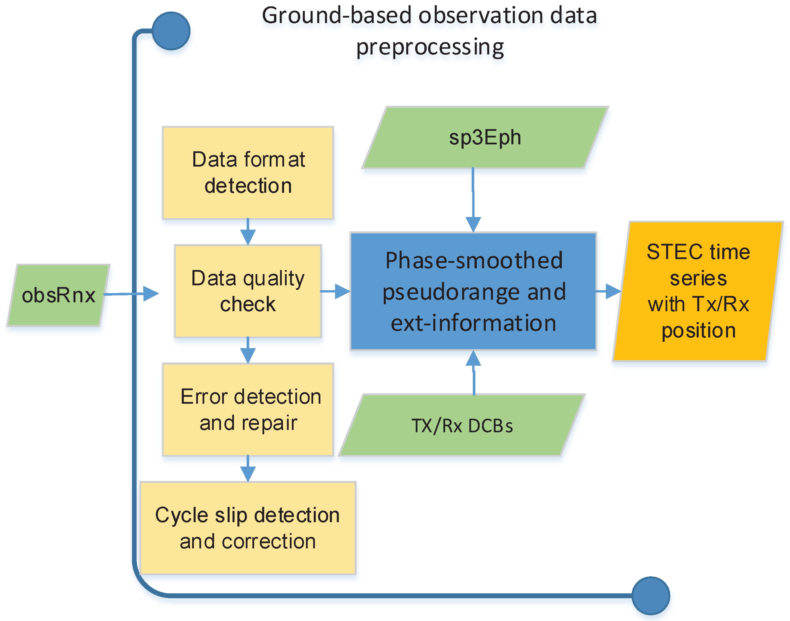
ftp://cddis.gsfc.nasa.gov/pub/gps/products). At the same time, it was necessary to prepare the ionospheric background field data; examples include data obtained from NeQuick, the IRI model or other empirical models. The rejection of carrier phase errors and the detection and repair of cycle slip were the key points of the processing of measured data. The data processing scheme consisted of the following steps. First, the ground-based observation data were merged and reformatted by TEQC, which was convenient for obtaining continuous results throughout the processing of observations within the selected time period. Second, data carrier gross errors and weekly jumps were detected and repaired. The specific process is shown in
Figure 3. However, the acquisition of accurate GNSS pseudorange and phase observations is still affected by many aspects, such as multipath errors and thermal noise errors. For this reason, generally, when ionospheric observations are obtained, more accurate pseudorange observations are obtained through pseudosmoothing following the processing steps mentioned above, after which the STEC data, including the receiver and the transmitter DCBs, are obtained by combining ionospheric data, that is, ground-based ionospheric observation data [
29,
30].
In the practical calculation process, the pseudosmoothed phase was usually obtained using the following weighted average recursion formula:
where
,
are the
ith,
th epoch smoothing pseudorange values;
are the corresponding phase observations;
are the corresponding phase wavelengths; and
is the
ith corresponding observed elevation angle.
The ionospheric residual combination was obtained through a formula computing the difference between observations at different frequencies:
where
;
and
are the frequencies of the satellite carrier;
c is the speed of light;
is the satellite differential code bias;
is the receiver differential code bias; and
denotes the slant total electron content on the receiver and satellite wires. During postprocessing, data can be obtained from either CODE or IGS products. COSMIC’s podTEC data were also obtained through the above process with phase observations of multifrequency data during LEO positioning. The data can be preselected by the STEC value and elevation angle and then assimilated as observation data with the top model proposed by Wu after sampling.
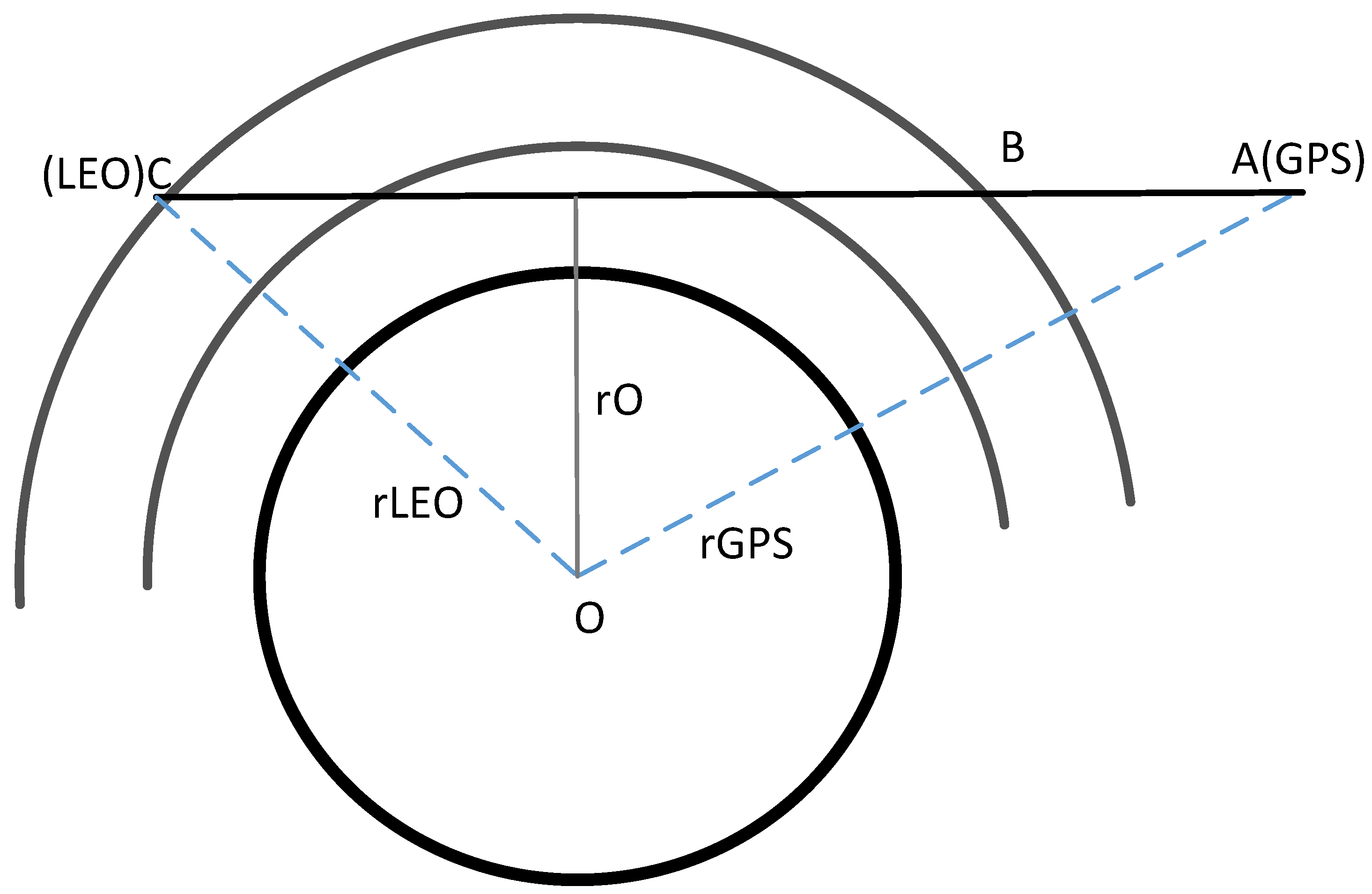
The acquisition of the calibrated TEC is illustrated in
Figure 4, from which we can find the following:
where
denotes the calibrated STEC;
is the occultation STEC; and
is the nonoccultation STEC corresponding to the AC segment. These variables can be obtained through the ground-based GNSS process with the phase observations of multifrequency data. In the occultation process, the time it takes for a LEO satellite to move from point C to point B is very short, and, thus, the distance of GNSS satellite motion is very short. We can assume that the ionospheric change along AB section is not significant, and the STEC of segment BC without DCB errors can be obtained; this segment is the influence of the ionosphere below the orbital height of the LEO satellite on signal propagation [
31].
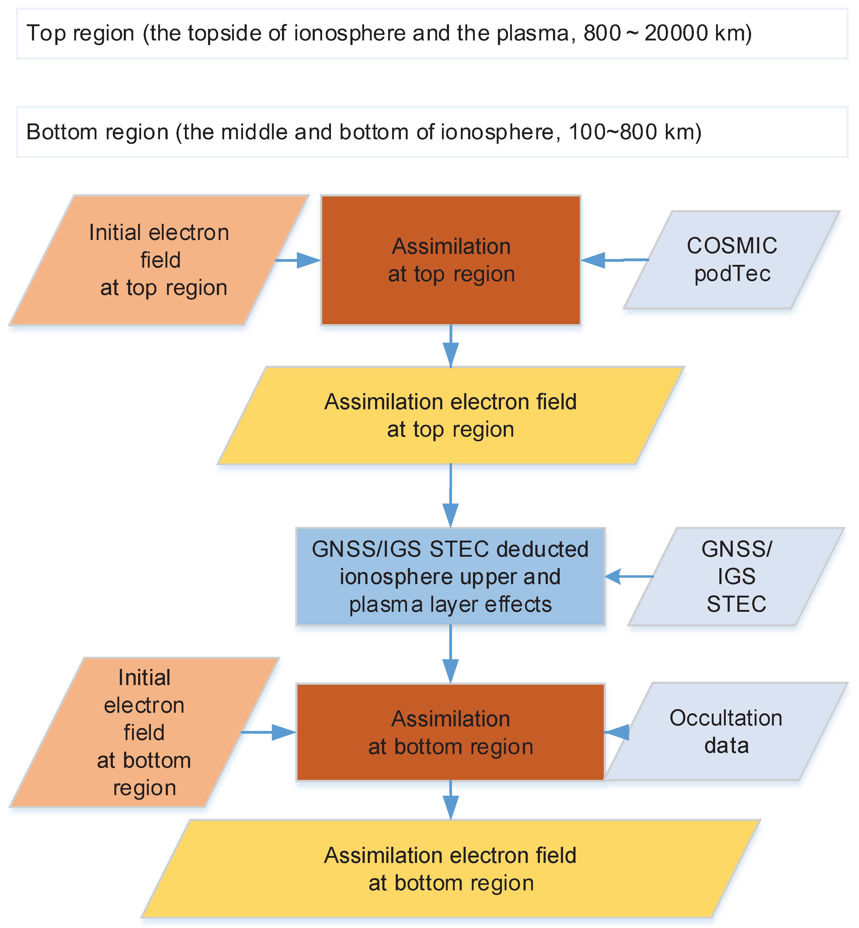
3.2. Data Processing Flow
Figure 5 shows the data processing workflow in the ionospheric assimilation process in this study. Due to the sparse and uneven distribution of ground stations and the height of GPS satellites (approximately 20,000 km), the ionospheric structure path distribution was presented as the cross shapes of cones whose apexes were ground-based stations or GPS satellites for the main part of the ionospheric assimilation using mainly ground-based GPS observation data, and the structural information was evenly distributed from 200 to 500 km, which is the range of the peak ionospheric height. The non-uniformity of the distribution information, especially in the top region, had a greater impact on the numerical solution in the assimilation; therefore, the top region and bottom region were selected for step-by-step assimilation. First, the assimilated model for the top region was obtained, as the podTec data improve the empirical model for the top region, from Wu et al. Then, the top region contribution was subtracted from the ground-based observation data, which was assimilated with the occultation observation data from the IRI or Wu et al.’s ionospheric model (called the IRI-Imp model) as the background field for the bottom region. Finally, a high-precision ionospheric model for the bottom region was obtained.
In the assimilation process, during the observation data screening process, the basic parameters were set as shown in
Table 1. As shown in
Table 1, we used the data (with sampling interval of 5 s) from the occultation observation system consisting of the GPS system (32 satellites) and the COSMIC satellites (a maximum of six), and the data (with sampling interval of 300 s) of the ground-based GNSS ionospheric observation system consisting of the GPS system and the stations (256 stations). During the assimilation, the grid height resolution was set along the distribution of the ionospheric electron density. In the top region, the altitude resolutions at 900–1000 km, 1000–2500 km and 2500–20,000 km were 100 km, 500 km and 2500 km, respectively. In the bottom region, the altitude resolutions at 100–220 km, 220–400 km, 400–700 km and 700–800 km were 40 km, 30 km, 50 km and 100 km, respectively.
3.3. Top Region Assimilation Process
The top region has an effect on the vertical total electron content (VTEC), which has a substantial influence on the ionospheric active period. Through the COSMIC project, we obtained access to a wealth of information on the top region. Wu et al. proposed obtaining the VTEC through COSMIC’s podTec hypothetical spherical shell mapping. Based on the electron density at the height of 800 km and assuming that the electron density diminished according to an exponential decay function, the parameter Hp related to the ionospheric decay rate at different mapping positions on the spherical shell can be calculated through the simultaneous VTEC expression and the electron density decay expression above 800 km. Finally, the electron density distribution of the ionosphere above 800 km was obtained.
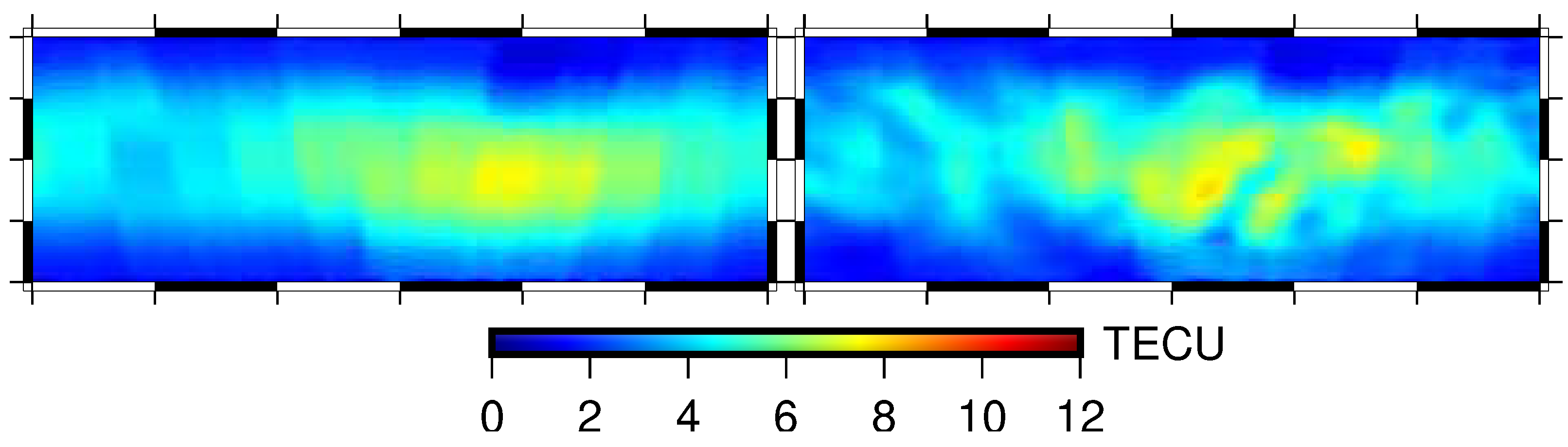
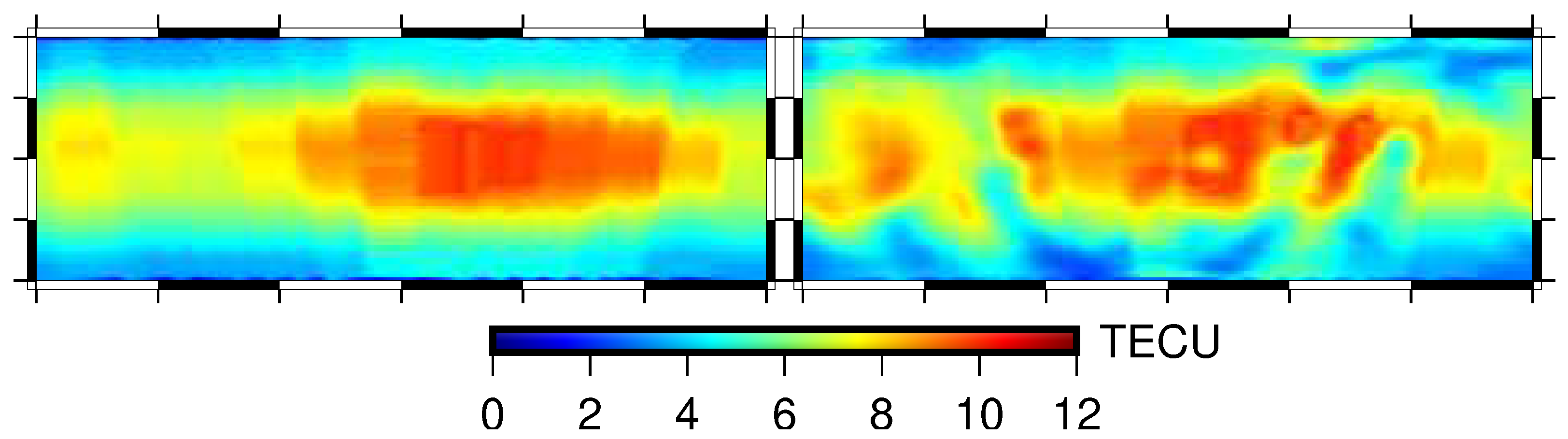
After the top region assimilation model was constructed from podTec data at 16:00–18:00 UTC on DOY 010, 2008 and DOY 089, 2012, the VTEC distributions in the top region along the geomagnetic latitude and longitude are shown on the left-hand side of
Figure 6 and
Figure 7. The top region was affected by solar energy and exhibited extremely obvious diurnal variation characteristics with an evident peak. As shown on the right-hand side of
Figure 6 and
Figure 7, after the assimilation of the top region, the VTEC distribution in the top region had a finer resolution, especially regarding the details of the peak.
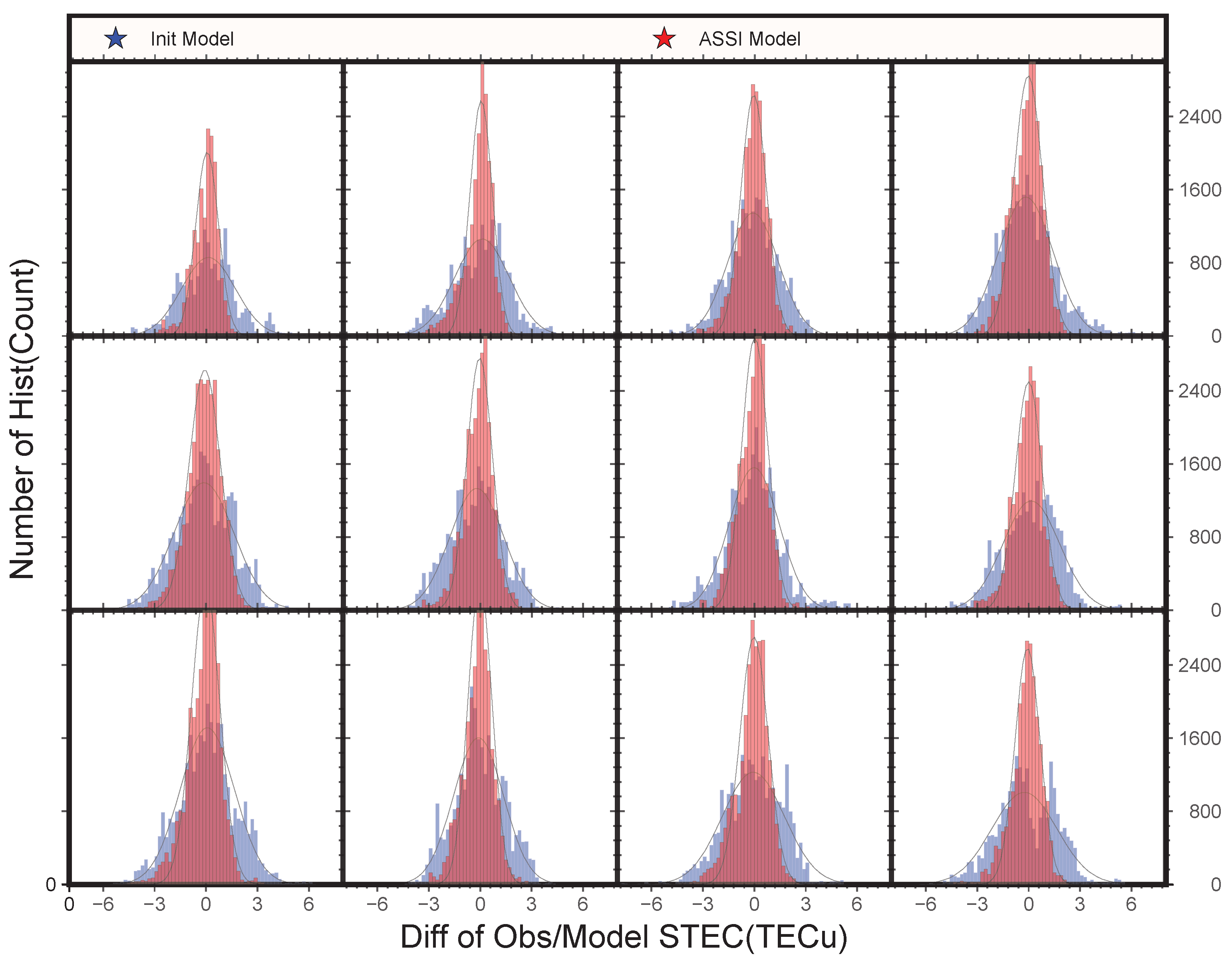
Figure 8 summarizes the distribution of the residual STEC between the podTEC observation and the top region model constructed by Wu et al.’s method or the top region assimilation model assimilated using podTec with the constructed model on DOY 010, 2008. After the step-by-step assimilation at the top region, the STEC error in the top region was greatly decreased. The residuals were distributed mainly within 4 TECU and were very close to the Gaussian distribution before and after assimilation. However, the residuals was more concentrated after assimilation, and the standard deviation was significantly decreased, which indicates the good performance of the step-by-step assimilation at the top region.
Occultation data were used for the top region to obtain a more accurate base for the electron density decay function with the altitude. The LEO satellite orbital height in the COSMIC project was approximately 800 km. Thus, the maximum value of the tangent point height of the calibrated TEC was close to the satellite orbital height, and could serve as the top constraint on the ionospheric assimilation at the bottom region, which could achieve consistency and continuity between the top and bottom regions assimilation models.
4. Validation
Both ground-based ionospheric observation data and occultation observation data were employed to ensure the structural and physical characteristics of the ionospheric model. The total amount of electrons on the signal path was compared with the total amount of electrons obtained by model integration, and these biases were reduced by weighting to correct the density of each cell in the ionospheric model along the signal path to achieve assimilation. The consistency between the STEC of the observed data and the integrated model STEC reflects the internal precision of the assimilation algorithm.
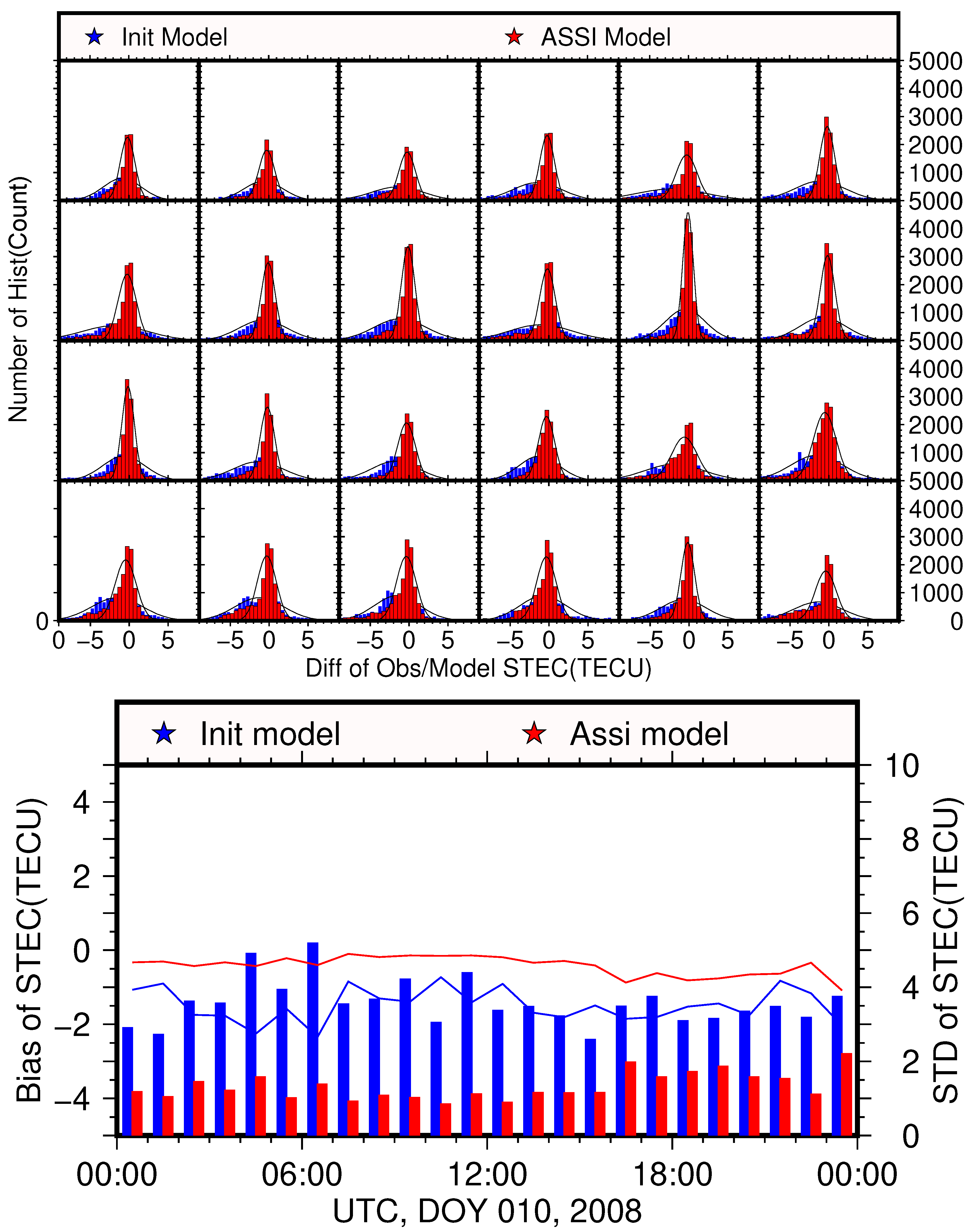
Figure 9 shows the error of the observed data on DOY 010, 2008 subtracted from the IRI model before and after assimilation with the corrected ground-based/spaceborne ionospheric data. The top panel shows the distribution of the residual STEC between the corrected ground-based/spaceborne ionospheric data and the IRI model of the bottom region or the model of the bottom region assimilated using the corrected ground-based/spaceborne ionospheric data with the IRI model on DOY 010, 2008. Although the IRI model could better describe the real-time ionospheric electron density distribution in the ionospheric quiet period, a large standard deviation still existed before the step-by-step assimilation at the bottom region. After the bottom assimilation, the residuals was more concentrated, and the standard deviation was significantly decreased.
After assimilation with the ground-based/spaceborne ionospheric data, the assimilation model was corrected. The biases of the ionospheric model STEC and the observed STEC data were significantly reduced, revealing small deviations in the residuals and Gaussian distributions with small standard deviations. The bottom panel of
Figure 9 shows the biases and standard deviations of the residuals of the observational data and the ionospheric model before and after the assimilation. This subfigure clearly illustrates that the STEC deviation was reduced from −1.5 to 2.0 TECU before the assimilation to −1.0 to 0.2 TECU after the assimilation, and the standard deviation was reduced from 3.0–4.0 TECU to 1.0–2.0 TECU, which constitutes an obvious improvement.
The two-part step-by-step ionospheric assimilation that considers the DCB errors of the instruments was applied with different observational data, and different strategies were defined by the observational data used in assimilation:
G: Only ground-based observation data
G+Cor: Only ground-based observation data with hypothesis correction
G/S+Cor: Ground-based/spaceborne observation data with hypothesis correction
The IRI model and the IRI-Imp model introduced by Wu et al. and their respective assimilation models ( IRI-Assi and IRI-Imp-Assi, respectively) through the “G”, “G+Cor”, and “G/S+Cor” strategy were obtained, and the verification of the consistency of assimilation results with various observational data in the ionosphere quiet period (DOY 010, 2008 is selected) and active period (DOY 089, 2012 is selected) were applied.
4.1. Validation with GIMs
To verify the improvements to the ionospheric model by the assimilation algorithm under different strategies, we performed a comparison between the IGS GIM and the assimilation results of the ionospheric quiet and active periods.
In
Table 2, on DOY 010, 2008, as the ionospheric quiet period, without pretreating the ionospheric top region or correcting for the hypothetical model error, although the VTEC deviation did not improve substantially, the standard deviation decreased from 1.71 TECU to 1.65 TECU. After deducting the influence of the top region of the ionosphere and correcting for the hypothetical model error, the VTEC deviation slightly increased, but the standard deviation greatly improved with a reduction of 0.25 TECU. The increase in occultation data increased the bias to −0.42 TECU (the deviation between the CODE and IGS was approximately 0.6 TECU), closer to that of the CODE model, and the standard deviation also significantly decreased by 0.08 TECU.
On DOY 089, 2012, as the active period of the ionosphere, the IRI model deviated greatly from the IGS GIM with a bias of −3.2 TECU and a standard deviation of 4.5 TECU. In the case of only ground-based ionospheric observation data, the strategy of preprocessing the top region and correcting for hypothetical model errors introduced the contribution of the top region; moreover, although the IRI introduced a significant correction to small real-world phenomena, the improvement to the standard deviation was not significant compared with the strategy of subtracting the influence of the top region of the ionosphere and correcting for hypothetical model errors. After introducing occultation observation data, which subtracted the influence of the top region of the ionosphere and corrected for hypothetical model errors, the assimilation deviation and standard deviation significantly improved.
Many different organizations provide GIM data; however, those organizations calculate DCBs and construct global ionospheric grids using different approaches, resulting in a deviation of 2–3 TECU and a root mean square error (RMSE) of 5–6 TECU among them. For this reason, if a GIM were used to validate the accuracy of the assimilation model, it would correspondingly be necessary to compare the GIMs among the different institutions. The GIM of the constructed model is a 13-order spherical harmonic function intended to fit a single-layer ionosphere with a spherical shell distribution. Similarly, the GIM from the European Space Agency (ESA) is also based on a spherical harmonic function to match the ionospheric distribution, whereas the GIM from the NASA Jet Propulsion Laboratory (JPL) is modeled using bicubic splines on a spherical grid, and the GIM from the IGS was obtained by the weighted combination of the ionospheric models of the CODE, ESA, Technical University of Catalonia (UPC), and JPL. Therefore, this study selected GIM data from the CODE, IGS, and JPL for comparison.
As shown in
Table 3, during the ionospheric quiet period, the IRI model was better able to characterize the real-time ionospheric distribution. The RMSE was within 2 TECU, which is closer to that of the GIM from IGS. For the assimilation performed by using the satellite orbit and DCB data released by CODE, the result was closer to the GIMs from CODE and IGS. However, JPL’s GIM gave greater RMSE values, meaning poorer performance even after assimilation, which indicates DCBs and its errors had a great impact on the assimilation result.
During the active period of the ionosphere, the IRI model displayed a large error. Compared with the JPL GIM, the RMSE was approximately 7 TECU. In the satellite orbit and DCB data released by CODE, the RMSE was 5.4 TECU, which was closer to the CODE GIM. After processing the ionospheric observation data, the assimilation results were significantly improved. Compared with the three models, the RMSE was improved by approximately 1.4 TECU, and the RMSE was only 4 TECU in comparison with the CODE GIM.
4.2. Validation with Ionosonde Observation
Ionospheric vertical altimeters emit pulse-modulated high-frequency radio waves vertically from the ground and receive the reflected signals of those waves at the same location. In this fashion, these altimeters can measure the time delay of the continuously changing frequency of radio waves and obtain the altitude distribution of the ionospheric electron density. The improvement effect of the assimilation algorithm on the ionospheric model was verified by observations (
ftp://ftp.ngdc.noaa.gov/ionosonde/) from ionospheric vertical altimeters that are automatic-scaled and manually checked.
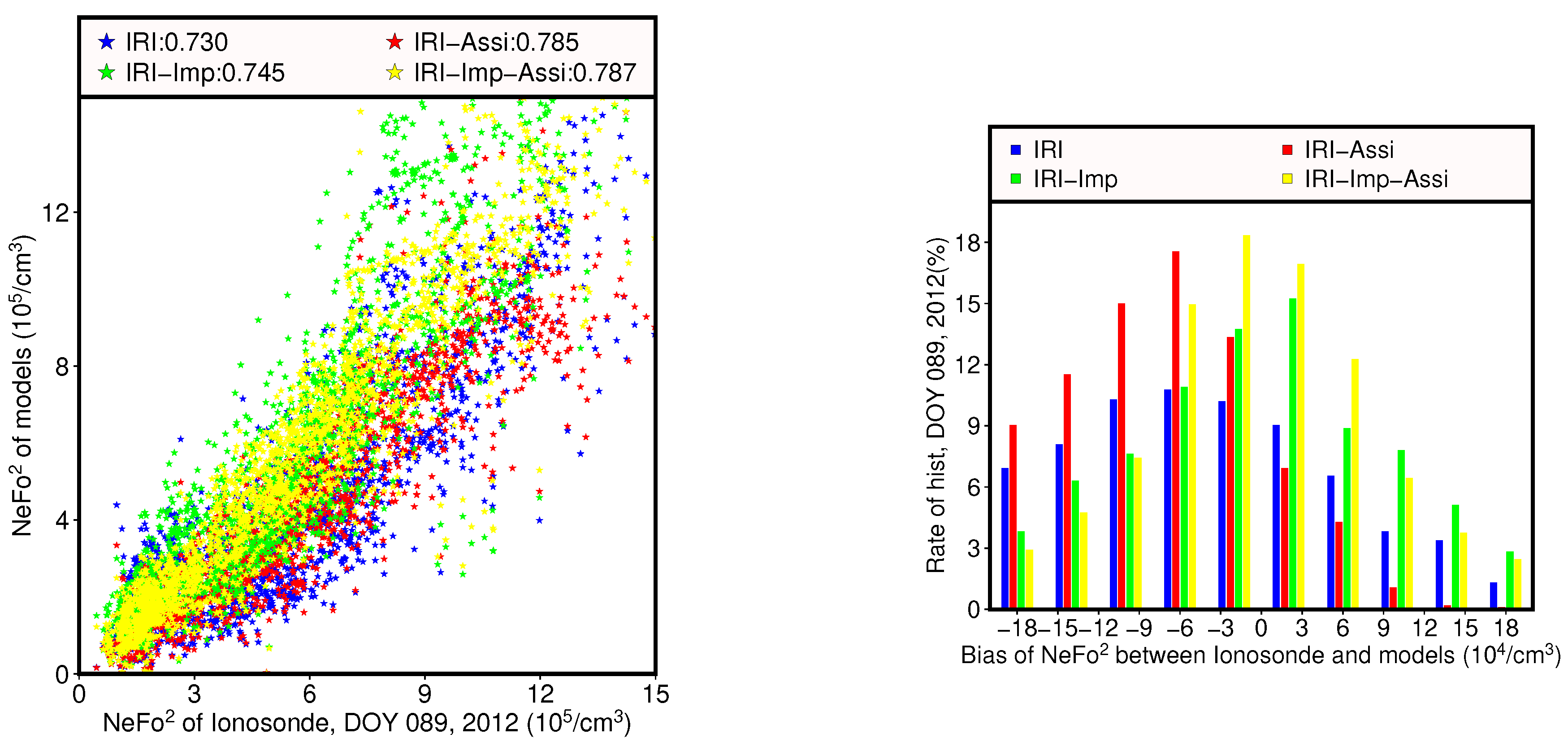
Compared with the ionosonde data, the assimilation results for these two days (DOY 010, 2008 and DOY 089, 2012) can lead to a consistent conclusion, and the improvement of data assimilation algorithms on DOY 089, 2012 was more significant, thus only the results of DOY 089, 2012 are described. The consistency between the IRI model and the IRI-Imp model introduced by Wu et al. and their respective assimilation models (IRI-Assi and IRI-Imp-Assi, respectively) through the “G/S+Cor” strategy are presented in
Figure 10 along with ionosonde data on DOY 89, 2012. The left subgraph demonstrates that the assimilation algorithm could correct the initial field, thereby making it more similar to the ionosonde observation data, and the degree of improvement was also very obvious in its correlation. The correlation of the IRI-Assi model increased from 0.730 to 0.785. In comparison with the IRI model, the correlation of IRI-Imp increased from 0.730 to 0.745, but the assimilation algorithm still increased the correlation of the assimilation results to 0.787. The right-hand subfigure illustrates that the bias of the IRI model was relatively small relative to that of the ionosonde data, but the assimilation algorithm increased the proportion of the smaller part of the error, indicating that the assimilation algorithm significantly improved upon the IRI-Assi model, while the IRI-Imp model was corrected by occultation data. Compared with the IRI model, the error was significantly reduced, but a large correction remained after assimilation, and the large deviation was obviously suppressed, thereby reducing the error.
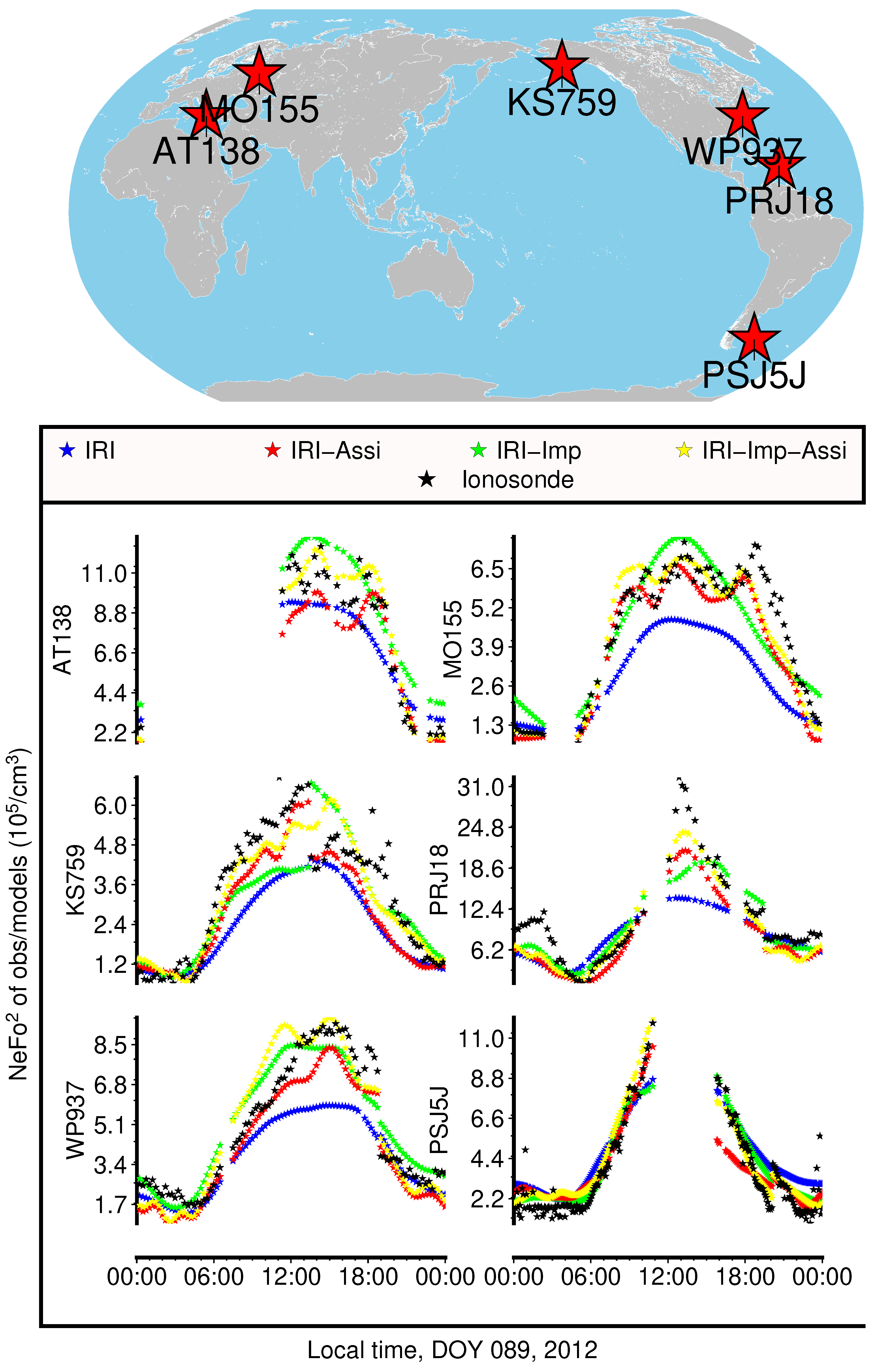
Ionosonde observation data and model peak density data from six ionosonde stations were selected, as shown in
Figure 11, and the variation in the electron density with local time was analyzed. As shown in the subfigures of
Figure 11, the IRI and IRI-Imp climate models could better conform to the variation in the ionosonde peak density with local time. At the same time, due to the remodeling of the peak density within Wu et al.’s method, the peak density of IRI-Imp better resembled the ionosonde data.
Through subgraphs of AT138, MO155, KS759 and WP937, the initial fields of the IRI and IRI-Imp models clearly added the influence of real-time observational data through the assimilation algorithm; consequently, the corresponding assimilation results displayed a diurnal variation of the ionosonde density peak data. Especially, in subgraphs of AT138 and MO155, the fluctuation of the ionosonde peak density of the two assimilation models around LT 15:00 was in great agreement with the fluctuation of the peak density of ionosonde.
Obviously, the peak density variation in the ionosonde data had greater volatility and was coarser than the assimilation models, as evidenced by multiple discrete green dots in subgraph of PSJ5J. Therefore, the results of the assimilation algorithm were more robust and should have higher credibility.
4.3. Validation with ISR Observation
According to the principle of electromagnetic wave scattering caused by random thermal fluctuations of the dielectric constant, the altitude range at which incoherent scattering could be detected was approximately 80–6000 km; this was accomplished by detecting the ionospheric characteristics from the ground with high-power radar. This detection process not only constitutes the most effective means of conducting research for ionospheric physics but also provides important information for dynamic investigations of the magnetosphere.
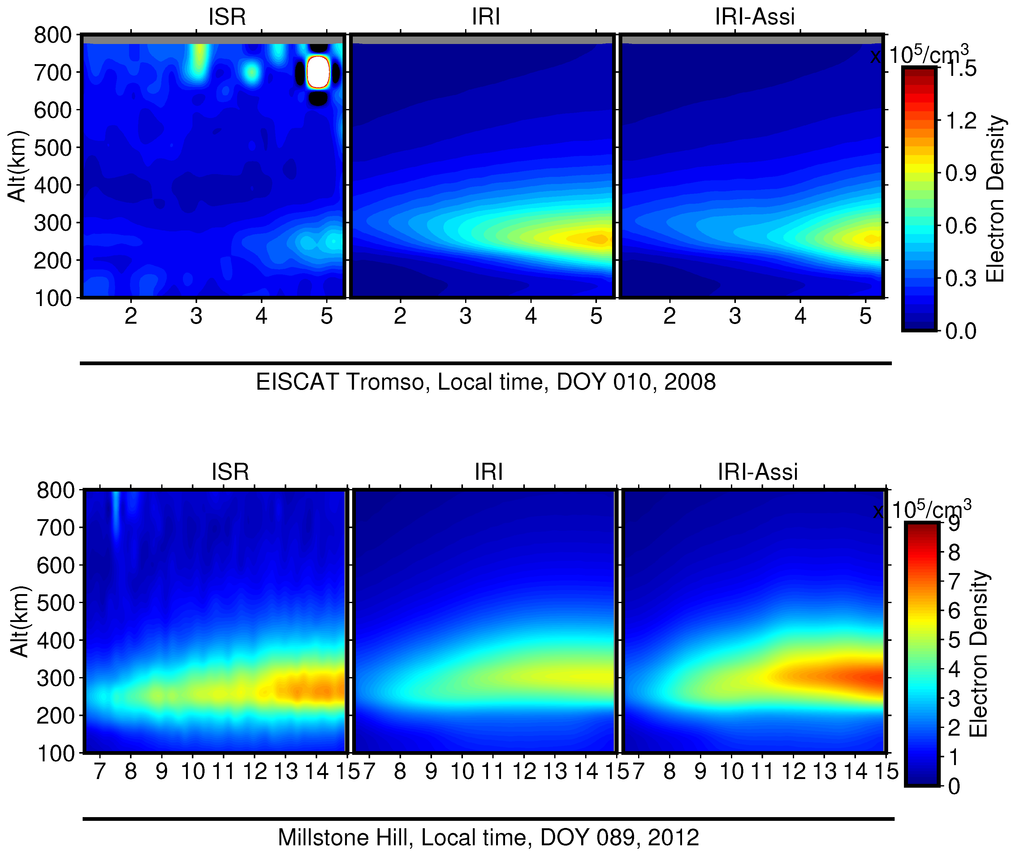
This study analyzed the IRI model and its assimilation model (IRI-Assi) through the “G/S+Cor” strategy along with the ISR observations of on DOY 010, 2008 at EISCAT Tromso and DOY 089, 2012 at Millstone Hill (of course, IRI-Imp model and IRI-Imp-Assi could be compared, but it was not necessary) to verify the stability of our proposed “two-part step-by-step ionospheric assimilation” algorithm. As shown in
Figure 12, a more accurate and detailed ionospheric model was obtained by the Kalman filtering assimilation algorithm. In details, on the upper panel of
Figure 12, which shows EDPs of the quiet ionosphere, the peak density in the IRI model was bigger, the peak height was smaller, and the F2 layer structure was clearer than in the ISR observations. After assimilation, the ionospheric peak density was significantly improved, and its shape and structure were closer to the ISR observations. However, the peak height correction was not obvious. The bottom panel of
Figure 12 is EDPs of the active ionosphere, which can get similar conclusions. Similar conclusions could be obtained from the results in
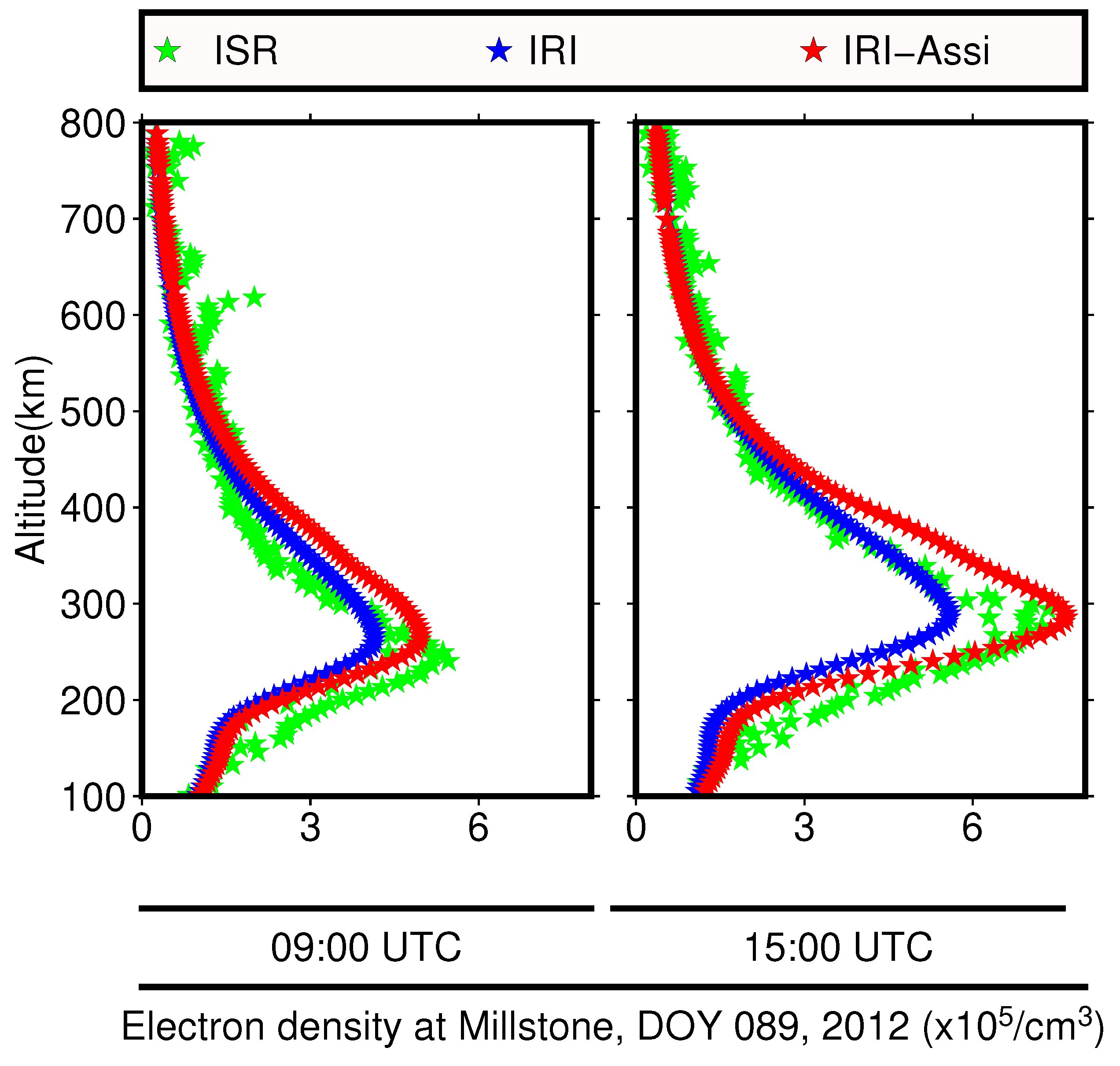
Figure 13. The left and right subfigures show Millstone’s EDP from ISR observations and the IRI model before and after assimilation at 09:00 and 15:00 local time. After the assimilation algorithm extended the initial field EDP, the peak density and peak height were closer to the feature points of the ISR observations. However, the correction process had little effect on the peak height of the EDP, which reduced the electron density of the assimilation model under the electron peak height and increased it above the electron peak height in comparison with the ISR observations.
4.4. Validation with Abel-Retrieved EDP
The EDP of ionPrf from CDAAC/UCAR was derived from the calculated excess phase file for each occultation using the Abel inversion algorithms with the local spherical symmetry hypothesis [
32], which can be used as a feasible reference for comparison.
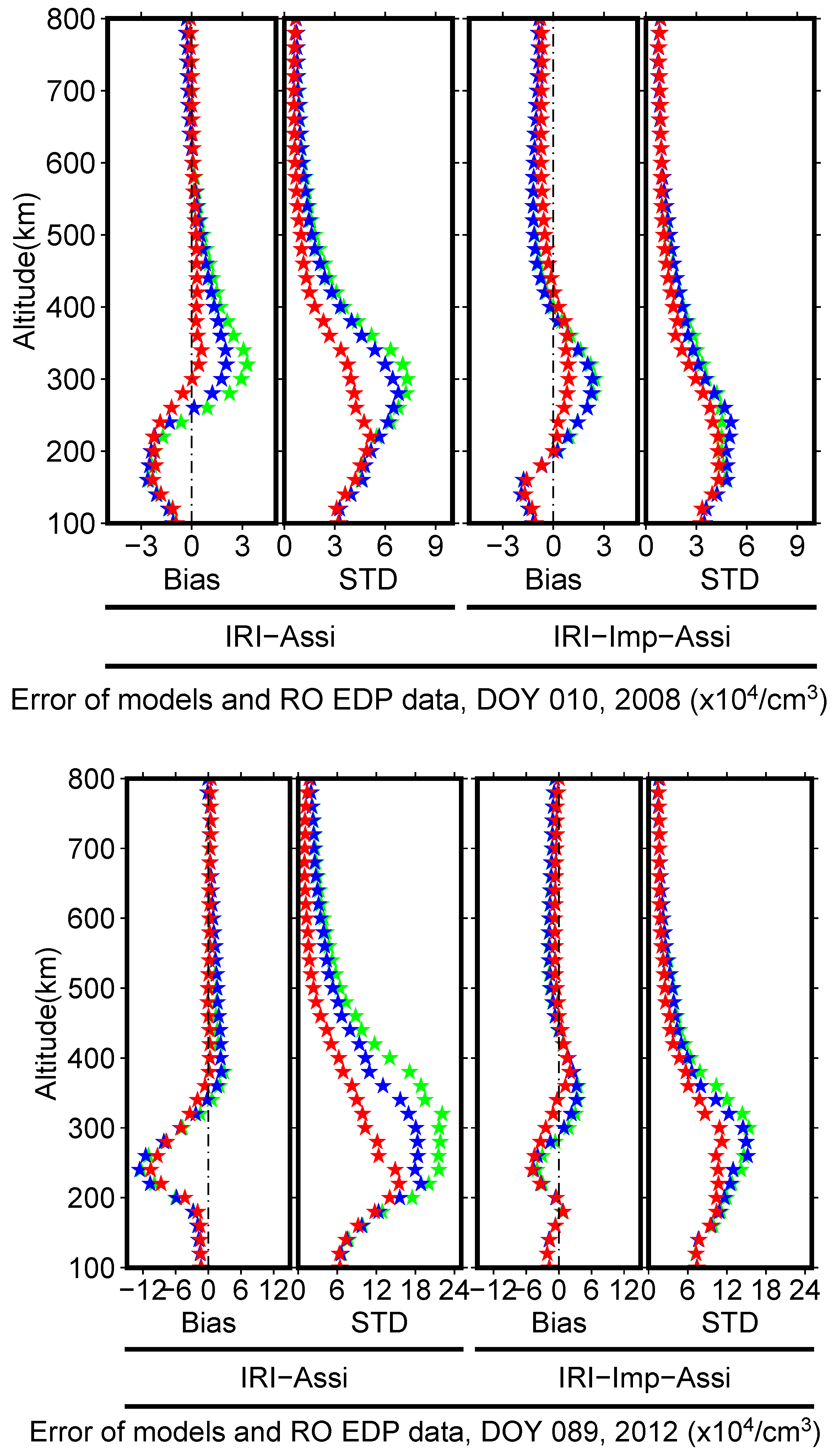
Using the EDP as a reference, the biases and standard deviations of the corresponding results from different assimilation strategies under different background fields are shown in
Figure 14 with the altitude during the ionospheric active and quiet periods. Taking left part of the upper panel of
Figure 14 as an example, the assimilation with the G+Cor strategy during the ionospheric active period was greatly improved compared with the initial IRI field. In particular, the bias and standard deviation in the peak height range (250–450 km) were extremely improved. The G/S+Cor strategy results showed a significant improvement in the deviation and standard deviation of the electron density above the peak height since the spatial distribution of the calibrated TEC structure information was concentrated in the region above the peak height of the ionosphere and because the Abel-retrieved EDP was obtained by using the calibrated TEC. Similarly, left part of the bottom panel of
Figure 14 demonstrates that the improvements to the assimilation results under the G+Cor and G/S+Cor strategies during the active period were consistent with those during the quiet period, but they were more significant in the former. Right parts of the upper and bottom panels of
Figure 14 show the deviations in the assimilation results from the EDP data under the G+Cor and G/S+Cor strategies with IRI-Imp as the background field. Clearly, the IRI-Imp was greatly improved compared with the IRI regardless of whether the ionosphere was in a quiet or an active period. However, IRI-Imp was corrected with occultation data, and the G+Cor strategy provided the IRI-Imp model with only terrestrial observations, and. thus, the assimilated results displayed a slight deviation from the initial field relative to the EDP. Some positive corrections could be observed in the case of large errors of the IRI and IRI-Imp models during the ionospheric active period. The results with the G/S+Cor strategy show that, even if the background field of the IRI-Imp model had corrected the ionospheric peak height and density by occultation observation data, the occultation data were attached to the assimilation and thus made significant corrections around and above the peak height of the ionosphere during its quiet and active periods; these findings confirm the idea that occultation horizontal structure information can improve IRI-Imp by assimilation.
5. Discussion
After verifying the accuracy of the KF algorithm with the influence of DCB through various data, we discuss the following two aspects through this algorithm. Firsts, we show the effect of the distribution assimilation algorithm on eliminating the influence of the top region, and discuss some details of the assimilation in different regions. Second, we show the effect of the introduction of multi-source data in the improved assimilation algorithm. In particular, the sensitivity of different background field data to occultation data is discussed.
5.1. Influence of Model Hypothesis’s Error on Ionospheric Assimilation Results
Hypothetical ionospheric model errors had a substantial influence on the ionospheric assimilation. In particular, the actual observation altitude range of the ionosphere was inconsistent with the altitude range of the assimilation result, and the influence of the top region was directly added to the assimilation model during the assimilation process for the bottom region. At the same time, the changes generated by the ionosphere during the assimilation time window and the errors in the grid representation were also transmitted to the assimilation results.
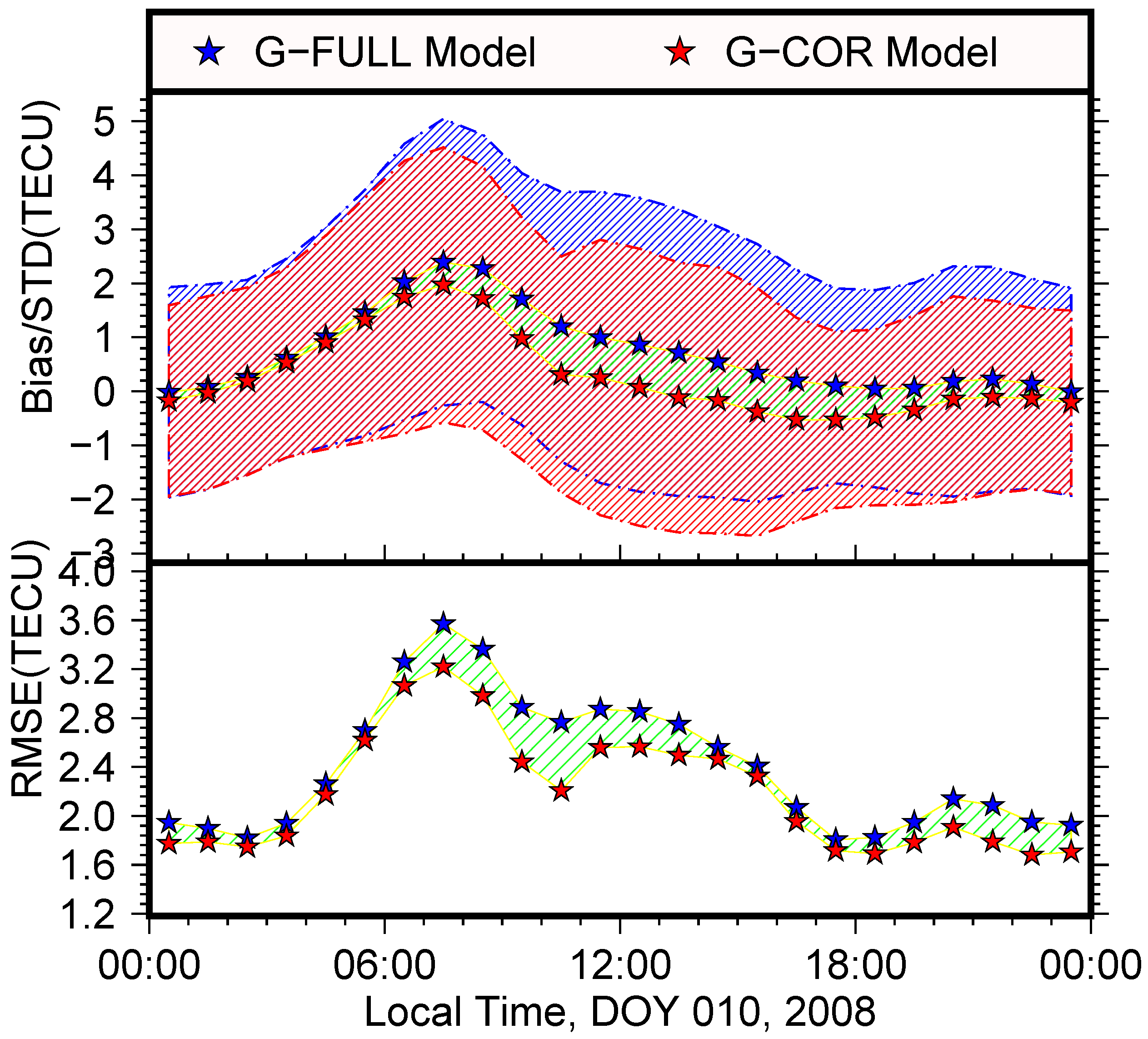
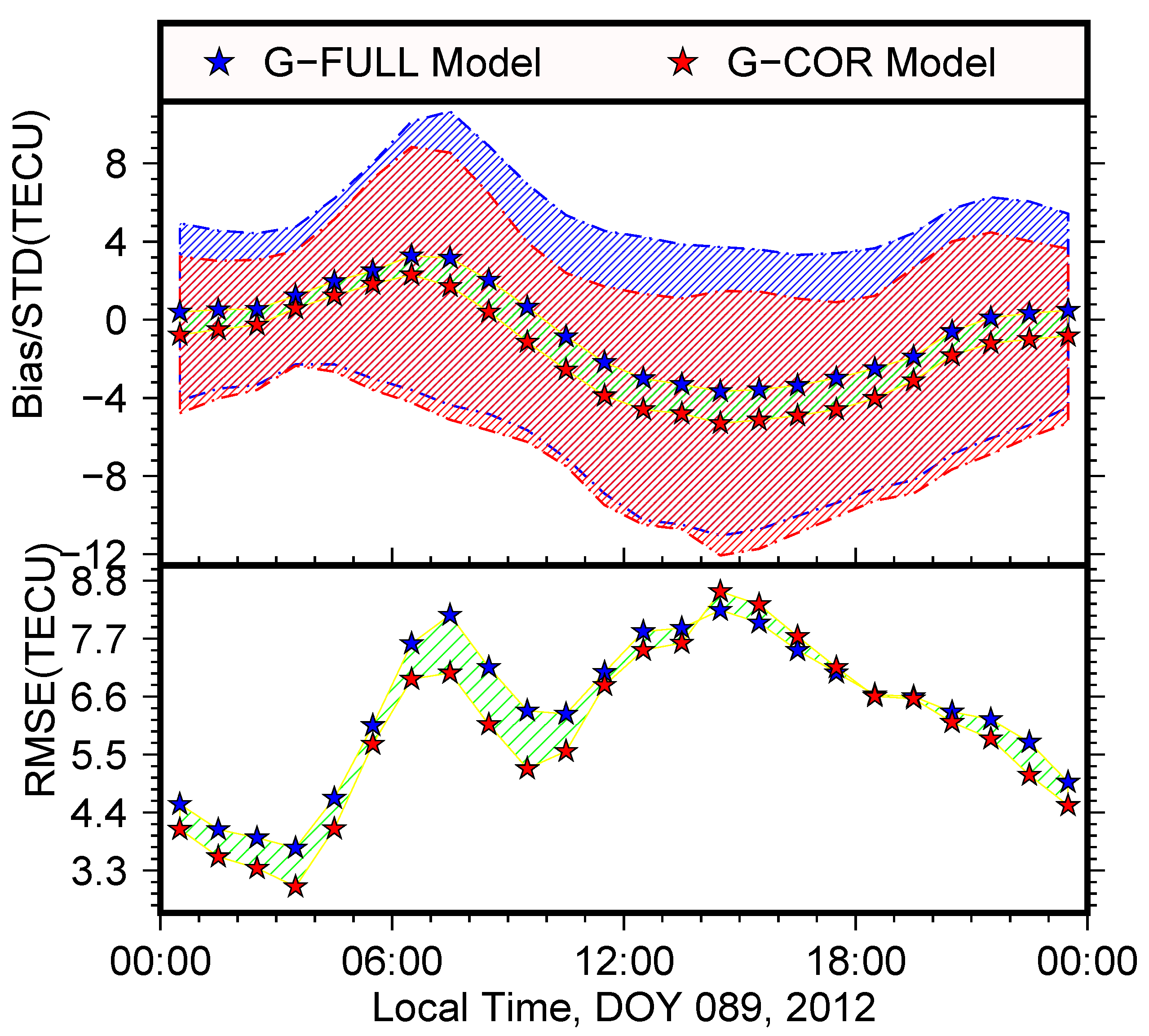
The upper and bottom subgraphs in
Figure 15 show the deviations and standard deviations of the VTEC between the ionospheric assimilation results and IGS GIM and the VTEC distributions on DOY 10, 2008 and DOY 89, 2012, respectively. During the ionospheric quiet and active periods, the assimilation results were obviously improved after the ionospheric hypothesis was subtracted from the observation data. The assimilation results under two strategies displayed a consistent bias trend with the local time, and the ionospheric assimilation results had a more stable error range and tended toward zero after the hypothetical model error was subtracted from the observations. At the same time, the RMSE was also greatly improved, and there was an improvement of approximately 1 TECU in both the active period and the quiet period of the ionosphere between 07:00 and 14:00 local time. The statistical results show that the assimilation results also had obvious improvement effects at night.
Comparing the upper and bottom subfigures of
Figure 15 reveals that the improvement strategy was more effective during the active period of the ionosphere. However, regardless of whether the ionosphere was in a quiet or an active period, the correction effect reached the maximum value between 10:00 and 12:00 local time, but this period was not the maximum time for ionospheric ionization (generally between 12:00 and 14:00 local time). This discrepancy may arise because solar radiation travels from the plasmasphere to the Earth’s surface, thereby affecting the top region first and then the bottom region. Thus, there was a significant correction between 10:00 and 12:00 local time. Generally, the ionospheric assimilation expressed the influence of the top region of the ionosphere by expanding the top of the empirical model, but the extended parameters were based on the peak density, peak height and elevation of the F2 layer, and these parameters were insufficient to reflect the ionospheric distribution features either horizontally or vertically at an altitude of 3000 km or above. Through distributed modeling, this problem could be effectively solved, and the electron density characteristics of the top region could be better described. Furthermore, with this method, the electron density structure of the middle and lower ionosphere could be obtained with a greater accuracy.
5.2. Sensitivity of Different Background Fields to Occultation Observation Data
Because GNSS ionospheric data lack ocean observations, we introduced spaceborne data for the assimilation, thereby avoiding excessive deviations caused by the absence of ocean data. Since 2012, the top boundary of the IRI has been corrected by neural networks or COSMIC occultation data; in contrast, the bottom of the ionosphere has been modeled based mainly on ground-based observation data. Therefore, it was necessary to optimize the ionospheric model by assimilation with occultation data from spaceborne observations. In the use of ionPrf from COSMIC, the ionospheric peak density, peak height and elevation were corrected by Wu et al. on the basis of IRI2007, and a modified IRI climate model was established; this climate model is named IRI-Imp in this paper. However, the bottom model was based on IRI2007, and ionPrf occultation data obtained by using Abel inversion algorithms based on the local spherical symmetry assumption were used as the modified input. In this process, the structural information of the ionosphere was lost during the acquisition of occultation observations, and spherical symmetry hypothesis errors were introduced. To this end, the occultation observation data were integrated with ground-based observation data in the assimilation method, and thus, the horizontal structure information in occultation observations could be better utilized.
We used two climate models as background fields to reconstruct the ionospheric 4D electron density distribution using a mix of ground-based/spaceborne observation data on DOY 10, 2008 and DOY 89, 2012. We used DCB data released by the CODE for the data processing. In addition, the IGS GIM was obtained by weighting ionospheric/related products based on different algorithms from the CODE, ESA, GPL, and UPC; the result was more informative. Therefore, we compared the assimilated ionospheric VTEC with the IGS and CODE GIMs, and the residual RMS statistics are shown in
Table 4.
Table 4 shows that the introduction of occultation data improved the accuracy of the assimilation model regardless of whether the ionosphere was in a quiet period or an active period. IRI-Imp had the best results due to its better spatial structure and shape. During the ionospheric quiet period, both IRI-Assi and IRI-Imp-Assi had relatively high precision, and the occultation data were not particularly significant for the improvement of either model. During the active period of the ionosphere, the ionospheric climate model displayed large errors. The lack of an occultation data correction in IRI2007 resulted in larger errors. Compared with IRI-Imp-Assi, due to the introduction of occultation data, the IRI-Assi model exhibited a greater reduction in error, as did the IGS and CODE GIMs.
The quality of GNSS ionospheric observation data is substantially affected by the distribution of IGS stations. Occultation observations are obtained on a global scale. Therefore, since the ionospheric assimilation model was very sensitive to the spatial distribution of occultation structure information, we calculated the sea–land RMSE of the ionospheric assimilation relative to the IGS GIM before and after the increase in occultation data. The results are shown in
Table 5.
On DOY 89, 2012, which was the active period of the ionosphere (as indicated by the red color), IRI2007 experienced a large deviation compared with the IGS GIM. Compared with the improvement in IRI-Imp-Assi, the improvement in IRI-Assi was greater on both land and sea, but it had a larger error than that in the quiet period of the ionosphere. On DOY 10, 2008, the IRI-Assi assimilation accuracy on land was higher than that of IRI-Imp-Assi, but the correction was not large. In comparison with IRI-Imp-Assi and IRI-Assi, the assimilation accuracy at sea was poor, but a more obvious improvement was observed referenced to the performance of that on land. This phenomenon occurred mainly for the following reasons. (1) IRI and IRI-Imp had a higher precision during the quiet period than during the active period of the ionosphere. (2) The bottom boundary of the ionosphere in IRI2007 was modeled based mainly on ground-based observation data, while IRI-Imp introduced occultation observations that greatly improved the precision in marine areas; hence, the former was more accurate on land than the latter, while the accuracy at sea was the opposite.
Furthermore, the occultation data more obviously improved the model without a correction of the occultation data in the case of a large ionospheric background field error; in particular, the improvement effect over marine areas was very obvious.
6. Conclusions
This study introduced a Kalman filter assimilation model that considers the DCB errors of GPS/LEO satellites and GPS stations. Through an internal STEC test and external validations with GIMs, ionosonde data, and ISR data, the improved algorithm was shown to greatly improve the ionospheric structure during the quiet and active periods of the ionosphere.
To establish the Kalman filter assimilation model considering the DCB errors of GPS/LEO satellites and GPS stations, we analyzed a correction for DCBs after introducing DCB errors from the receiver and the transmitter and found that the improved assimilation method can effectively suppress DCB errors caused by the single-layer hypothesis, further reducing the impacts of observed STEC errors on the assimilation process.
By performing multisource observation data assimilation and performing internal verification and external checks of multisource ionospheric data obtained by different means, the ionospheric model was effectively expressed by the assimilation algorithm, and it was more consistent with multisource observations than with background fields, such as the IRI model. Through a comparison with various GIMs, the assimilation algorithms were more effective during the active period than during the quiet period of the ionosphere. Compared with ionosonde observations, the assimilation results not only were greatly improved than the initial models but also added to the daily variation of the ionosonde data. Based on ISR data, the influence of the assimilation algorithm on the electron density structure affected mainly the improvement in the peak density, while it had a weak effect on the peak height, which is consistent with Fu et al.’s result [
18]. Finally, a comparison with the Abel-retrieved EDP from CDAAC/UCAR demonstrated that the result from the G/S+Cor strategy using the calibrated TEC from occultation data was more consistent than that from the G+Cor strategy.
Under the above reliability tests, this paper discusses the following two points:
- (1)
Influence of hypothetical model errors on the ionospheric assimilation results.
When using hypothetical corrections on ground-based/spaceborne observation data, the assimilation had a significant improvement, especially in the ionospheric active period. By means of the two-part step-by-step assimilation, the electron density characteristics of the top region can be better characterized, and the electron density structure of the middle and lower ionosphere can be obtained with a greater accuracy.
- (2)
Sensitivities of different background fields to occultation observation data from GIM models produced by different data centers.
The occultation data had a more obvious improvement effect on the model without a correction of the occultation data in the case of a large background field error for the ionosphere; in particular, the improvement effect in marine areas was very obvious.
Finally, more work can be carried out. The stability of the coupling method that the plasmasphere is divided into two parts to study the relationship between them requires testing data for a longer period of time. It could be applied to the ionospheric magnetic storm process or the special event (such as earthquake and eclipse process) on the study of the ionosphere. Our algorithm temporarily uses the “3D-FGAT” mode, which means that each assimilation process is independent. In the future, we will consider introducing SAMI3 [
3] to promote the assimilation of the previous step into the next moment, to achieve dynamic evolution and assimilation.


