Article

An Improved Approach Considering Intraclass Variability for Mapping Winter Wheat Using Multitemporal MODIS EVI Images

1
International Institute for Earth System Science, Nanjing University, Nanjing 210023, China
2
Department of Plant and Soil Sciences, College of Agriculture, Food and Environment, University of Kentucky, KY 40546, USA
3
(Retired) Division of Geographic Information, Commonwealth Office of Technology, Frankfort, KY 40601, USA
4
Department of Earth and Environmental Sciences, Murray State University, Murray, KY 42071, USA
5
Key Laboratory of Ecosystem Network Observation and Modeling, Institute of Geographic Sciences and Natural Resources Research, Chinese Academy of Sciences, Beijing 100101, China
*
Author to whom correspondence should be addressed.
Remote Sens. 2019, 11(10), 1191; https://0-doi-org.brum.beds.ac.uk/10.3390/rs11101191
Submission received: 8 March 2019 / Revised: 13 May 2019 / Accepted: 16 May 2019 / Published: 19 May 2019

Abstract

:
Winter wheat is one of the major cereal crops in the world. Monitoring and mapping its spatial distribution has significant implications for agriculture management, water resources utilization, and food security. Generally, winter wheat has distinguished phenological stages during the growing season, which form a unique EVI (Enhanced Vegetation Index) time series curve and differ considerably from other crop types and natural vegetation. Since early 2000, the MODIS EVI product has become the primary dataset for satellite-based crop monitoring at large scales due to its high temporal resolution, huge observation scope, and timely availability. However, the intraclass variability of winter wheat caused by field conditions and agricultural practices might lower the mapping accuracy, which has received little attention in previous studies. Here, we present a winter wheat mapping approach that integrates the variables derived from the MODIS EVI time series taking into account intraclass variability. We applied this approach to two winter wheat concentration areas, the state of Kansas in the U.S. and the North China Plain region (NCP). The results were evaluated against crop-specific maps or statistical data at the state/regional level, county level, and site level. Compared with statistical data, the accuracies in Kansas and the NCP were 95.1% and 92.9% at the state/regional level with R2 (Coefficient of Determination) values of 0.96 and 0.71 at the county level, respectively. Overall accuracies in confusion matrix were evaluated by validation samples in both Kansas (90.3%) and the NCP (85.0%) at the site level. Comparisons with methods without considering intraclass variability demonstrated that winter wheat mapping accuracies were improved by 17% in Kansas and 15% in the NCP using the improved approach. Further analysis indicated that our approach performed better in areas with lower landscape fragmentation, which may partly explain the relatively higher accuracy of winter wheat mapping in Kansas. This study provides a new perspective for generating multiple subclasses as training inputs to decrease the intraclass differences for crop type detection based on the MODIS EVI time series. This approach provides a flexible framework with few variables and fewer training samples that could facilitate its application to multiple-crop-type mapping at large scales.

Graphical Abstract

1. Introduction

Wheat is the world’s third largest food crop in terms of production [1] and is the most widely grown crop globally [2]. The wheat growing area covers over 200 million hectares worldwide [3], with winter wheat accounting for more than 80% [4]. Maintaining and increasing global winter wheat production is strongly linked to food security [5,6,7,8]. Accurate and timely information of temporal and spatial variations in winter wheat areas is therefore essential for crop yield estimation, climate impacts assessment, and agricultural policy-making [9,10].
The development of the remote sensing technology makes it possible to monitor crop areas at fine spectral, temporal, and spatial scales realistically [11,12]. Specifically, data with high temporal resolution provides time-series images with daily signatures and has been successfully used for crop area monitoring [13,14,15]. Previous studies have shown that optical satellite remote sensing is a viable means to detect winter wheat fields over large-scale and longtime series [4,15]. The Moderate Resolution Imaging Spectroradiometer (MODIS) on board the NASA Earth Observing System Terra and Aqua satellite platforms offers unprecedented capabilities for large-area crop mapping by providing global coverage, half-day revisit capacities, and medium spatial resolution [16,17]. MODIS Vegetation Index (VI) time-series has been proven to be a powerful tool for crop type characterization and has been successfully used for crop mapping across a wide range of scales and geographic locations [18,19]. Some studies have used the MODIS VI data for mapping and monitoring winter wheat across different scales [15,20].
Recently, a variety of algorithms combined with specific features (e.g., spectral, temporal, and phenological features) have been employed in remote sensing-based crop mapping, such as Parallelepiped Classifier [21], Minimum Distance [22], Maximum Likelihood [23], Spectral Angle Mapper [24], Support Vector Machines [25,26,27], Neural Network Classifier [24], Classification and Regression Trees (CARTs) [28], etc. Many factors may act to affect the remote sensing-based mapping accuracy, in which training samples have a more significant impact than the mapping techniques [26,29,30]. For a given crop type, the upper and lower bounds thresholds of training datasets mainly depend on intraclass variability, which results from differences in crop environmental status and management practices [14]. Different growth conditions and landscape factors (e.g., irrigation, fertility, climate, topography, fragmentation) may cause intraclass differences affecting the spectral signatures of the same crop type [31]. Intra- and interclass confusion due to these factors would degrade the ability of the image classifier to produce accurate maps for specific crop types.
Until now, few studies for winter wheat mapping have considered the intraclass features at different stages with different conditions, which might introduce large uncertainties in estimating and mapping crop area [8,14,17]. An approach considering the intraclass variability of winter wheat is therefore needed to generate the timely and reliable information on crop mapping areas, which will benefit for ensuring food security in the face of crop yield gaps, climate change, and extreme climate events.
The global cropland datasets showed the spatial distribution of cropland at 30 m spatial resolution, but it did not classify specific crop types [32]. For the United States, the 250 m MODIS-based crop types distribution were developed for the period 2001–2013, but did not separate wheat into winter wheat and spring wheat [33]. This situation justifies the importance of this study. Therefore, a robust approach for winter wheat mapping at the regional scale is highly needed.
In this study, an improved approach for mapping winter wheat based on intraclass variability was presented that integrated the angles and distances of multidimensional vectors and adopted multiple subclasses as training samples. The presented approach was used for mapping winter wheat based on the MODIS EVI time series data in two study areas; Kansas and the North China Plain region (NCP). Kansas has large areas of consecutive wheat fields which generally range from 30 to 150 ha and has a comprehensive and reliable county-level archive of crop statistics [4]. The NCP accounts for approximately two-thirds of China’s total wheat area and production [34], representing the most important wheat-producing area in China. Reference data at the administrative level, county level, and site level are also available in this region.
The objectives of this study are to (1) present an improved approach considering intraclass variability for winter wheat mapping based on the MODIS EVI time series images; (2) apply the new approach to two areas of interest, Kansas and the NCP; (3) analyze the effects of landscape structure on remote sensing-based crop mapping accuracy using two landscape metrics, i.e., Fragmentation Index (FRG) and Percentage of the Landscape (PLAND); and (4) identify the uncertainties and future needs in remote sensing-based crop area mapping.

2. Study Area and Datasets
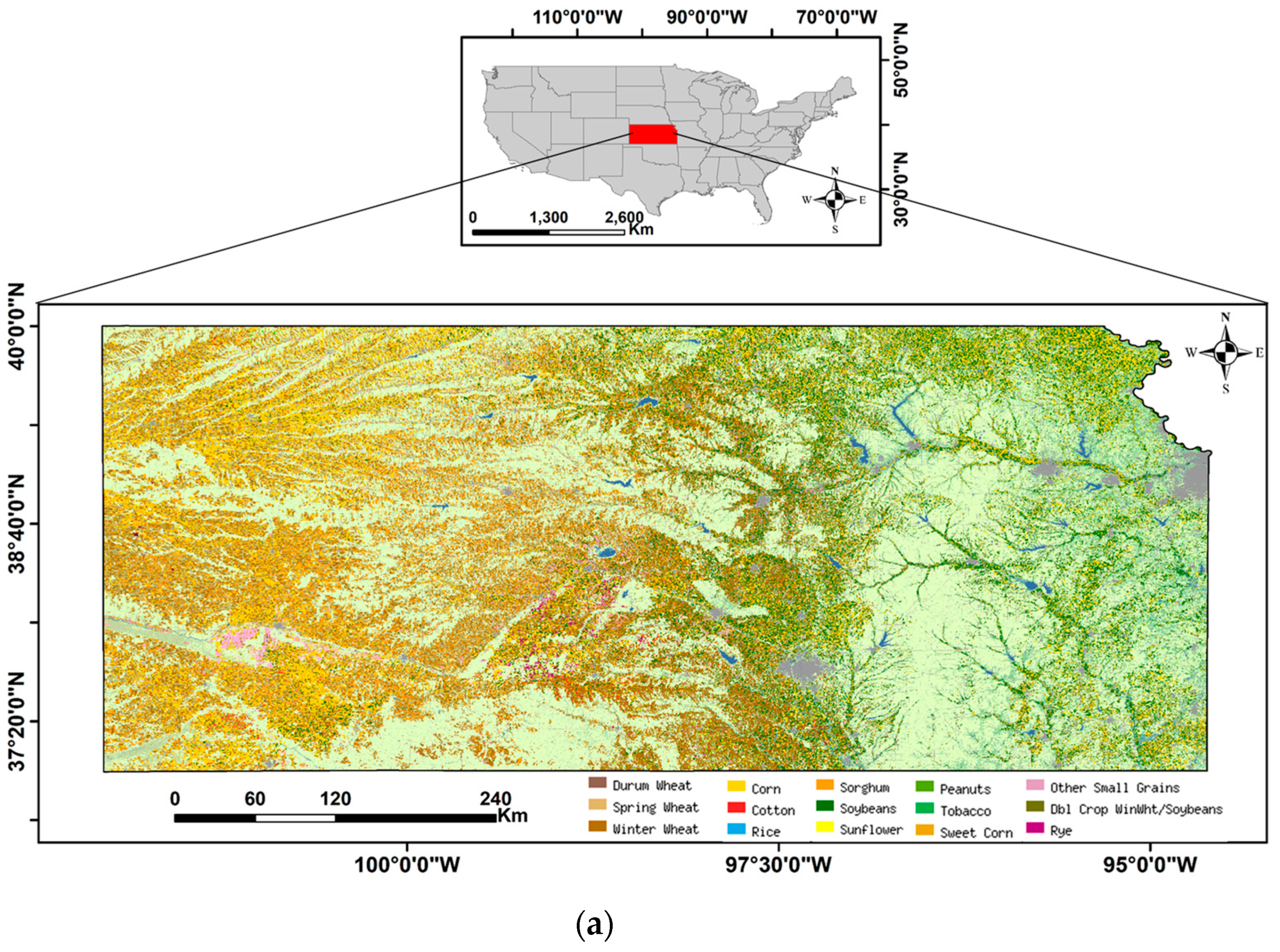
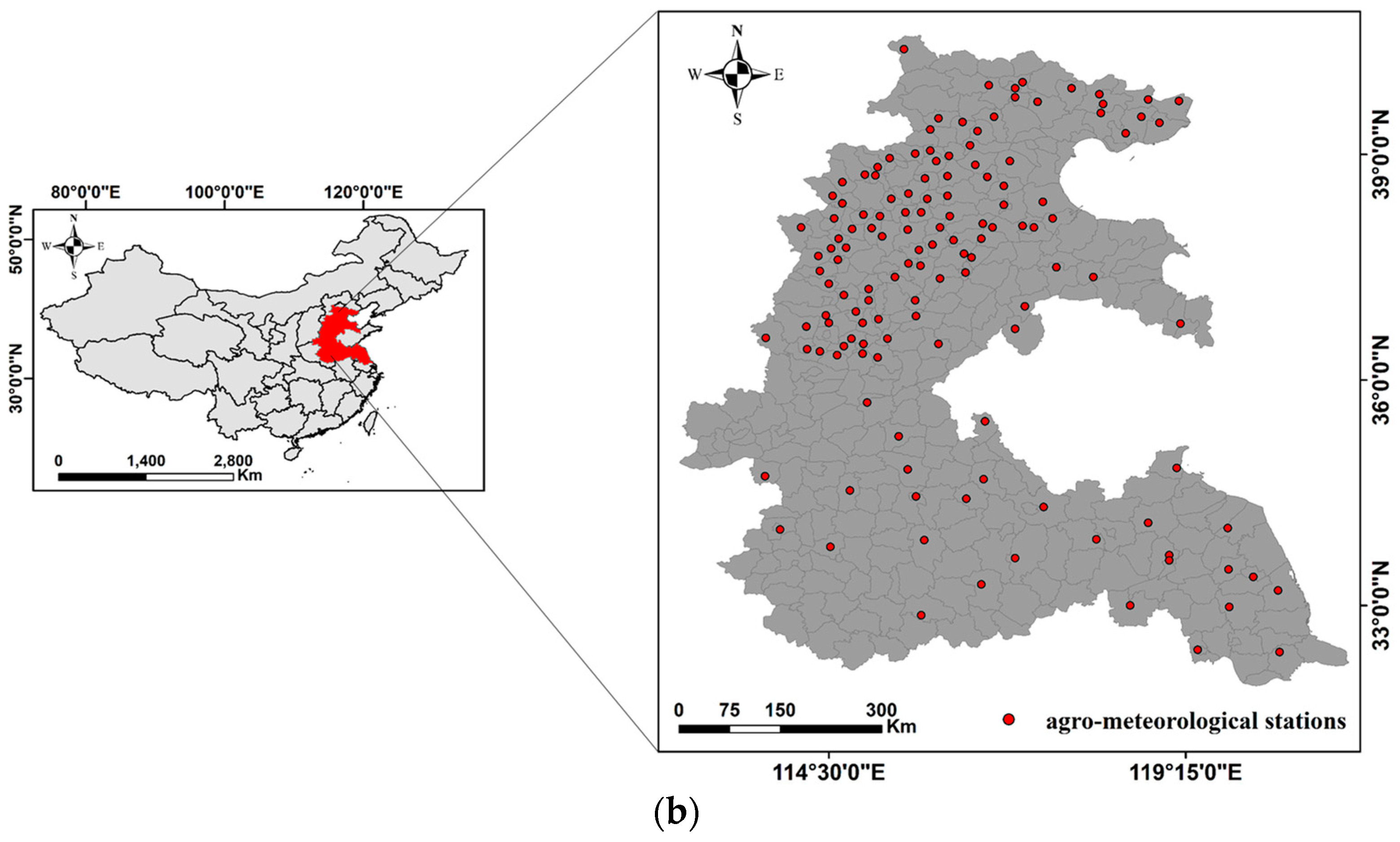
2.1. Study Area

Two major winter wheat dominant areas, i.e., Kansas, USA (94–102°W and 37–40°N) (Figure 1a) and the NCP, China (111–123°E and 33–41°N) (Figure 1b), were selected as the regions of interest. Most US wheat is grown in the Great Plains from Texas to North Dakota, accounting for about 75% of national wheat production (http://www.fao.org/docrep/006/y4011e/y4011e04.html). About 41% of the total US wheat production is of the Hard Red Winter (HRW) class, and most HRW wheat is grown in the central and southern Great Plains states. Kansas lies in the heart of the central Great Plains region and is one of the major winter wheat producing states in the Great Plains [35]. The NCP is the largest agricultural area in China [36], also known as the “breadbasket of China”, accounting for about 71% of the country’s wheat production [34,37,38,39]. It covers two metropolises (Beijing and Tianjin) and five provinces (i.e., Anhui, Hebei, Henan, Jiangsu, and Shandong) [40].
Kansas has a temperate continental climate with a strong east-west precipitation gradient and a strong north-west-south-east temperature gradient. The annual mean precipitation ranges from < 450 mm in the west to > 1,200 mm in the southeast, whereas the annual mean temperature varies from < 11 °C in the northwest to > 15 °C in the southeast. On the NCP, the elevation is less than 50 m above sea level [34]. The plain has a temperate, subhumid, and continental monsoon climate [41]. The annual rainfall varies between 480 mm in the north and 850 mm in the south of the NCP [10]. The annual mean temperature is around 12.2 °C [38], while the minimum (January) and maximum (July) monthly average temperature were −6 to 0 °C and 25 to 28 °C, respectively [39].

2.2. Datasets

2.2.1. Remote Sensing Data

The MODIS (Moderate Resolution Imaging Spectroradiometer) instrument is operational on both the Terra spacecraft (launched on December 1999, overpassing the equator about 10:30 am) and the Aqua spacecraft (launched on May 2002, overpassing the equator about 1:30 pm). In this study, 16-day 250 m MODIS EVI product (MOD13Q1) was obtained from the Land Processes Distributed Active Archive Center (LPDAAC) (http://lpdaac.usgs.gov/) [19]. The h09v05, h10v04, and h10v05 tiled grid data for Kansas were collected from the day of year (DOY) 257 (2016) to 193 (2017). The h26v04, h26v05, h27v04, h27v05, and h28v05 tiled grid data were downloaded for the period DOY 273 (2011) to DOY 177 (2012) for the NCP. The MODIS EVI products were geometrically, atmospherically, and bidirectional reflectance distribution function (BRDF) corrected, validated, and quality assured through the EOS program [42,43].

2.2.2. Crop Distribution Data

To train and validate the proposed approach, we collected the Cropland Data Layer (CDL) from CropScape (http://nassgeodata.gmu.edu/CropScape/), developed by the United States Department of Agriculture National Agricultural Statistics Service (USDA-NASS). The spatial resolution of the CDL varies from 30 to 56 m, depending on the imagery source [33,44]. Winter wheat was mapped at an annual interval since 2006 for Kansas, with overall accuracies over 90% for both producer’s accuracy and user’s accuracy in 2017 CDL (https://www.nass.usda.gov/Research_and_Science/Cropland/metadata/metadata_ks17.htm). The producer’s accuracy is a measure of the omission error and is defined as the number of correctly classified pixels of the class relative to the total number of pixels of that class used in the assessment. The user’s accuracy is a measure of the commission error associated with a class, which is derived from the number of pixels correctly allocated to a class relative to the total number of pixels predicted to belong to that class [45]. For this study, we used 2017 USDA CDL for Kansas as the reference map (Figure 1a), which provided the training and verification samples at the site level. For the NCP, no such crop cover data is available.

2.2.3. Statistical Data and Agrometeorological Stations Data
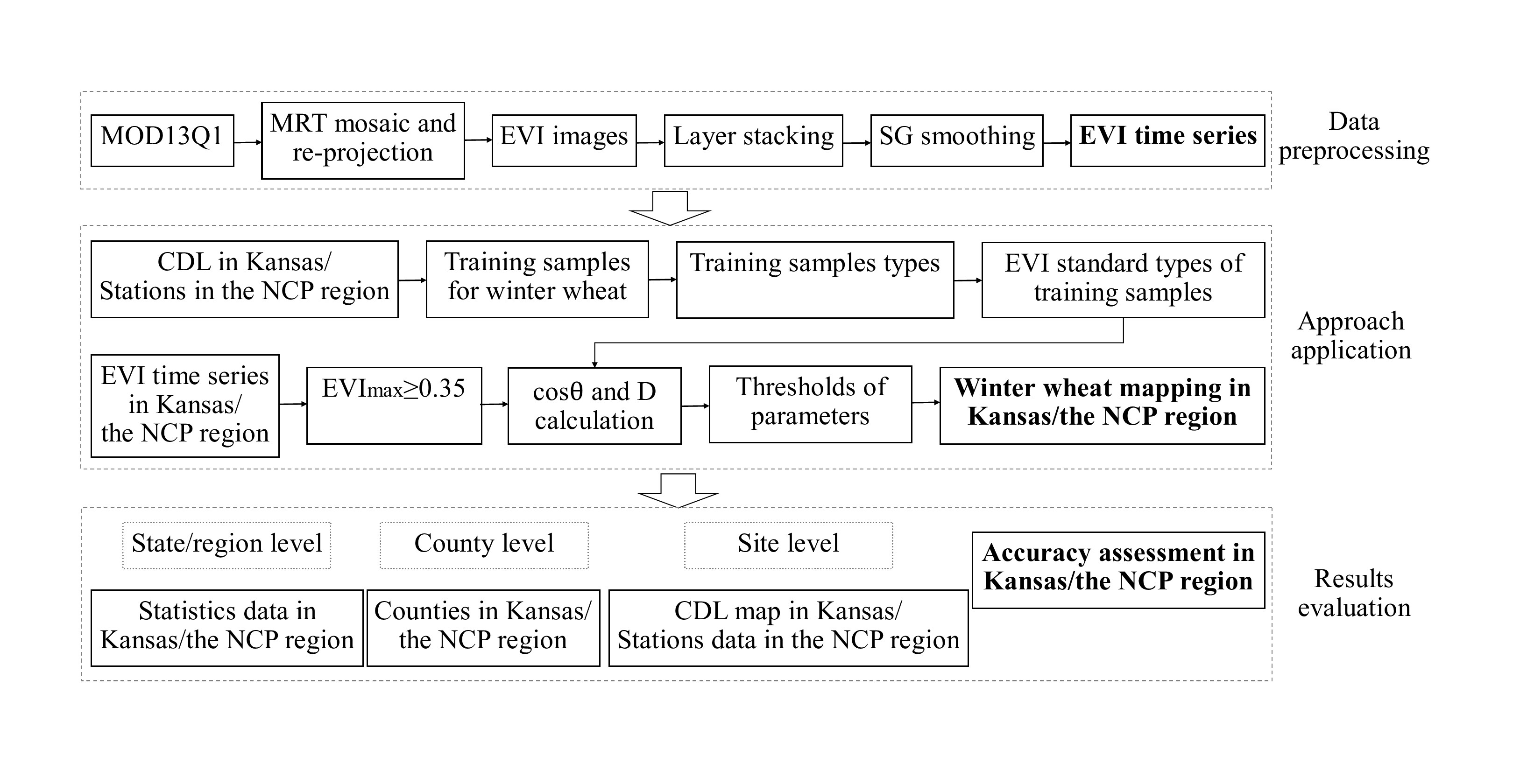
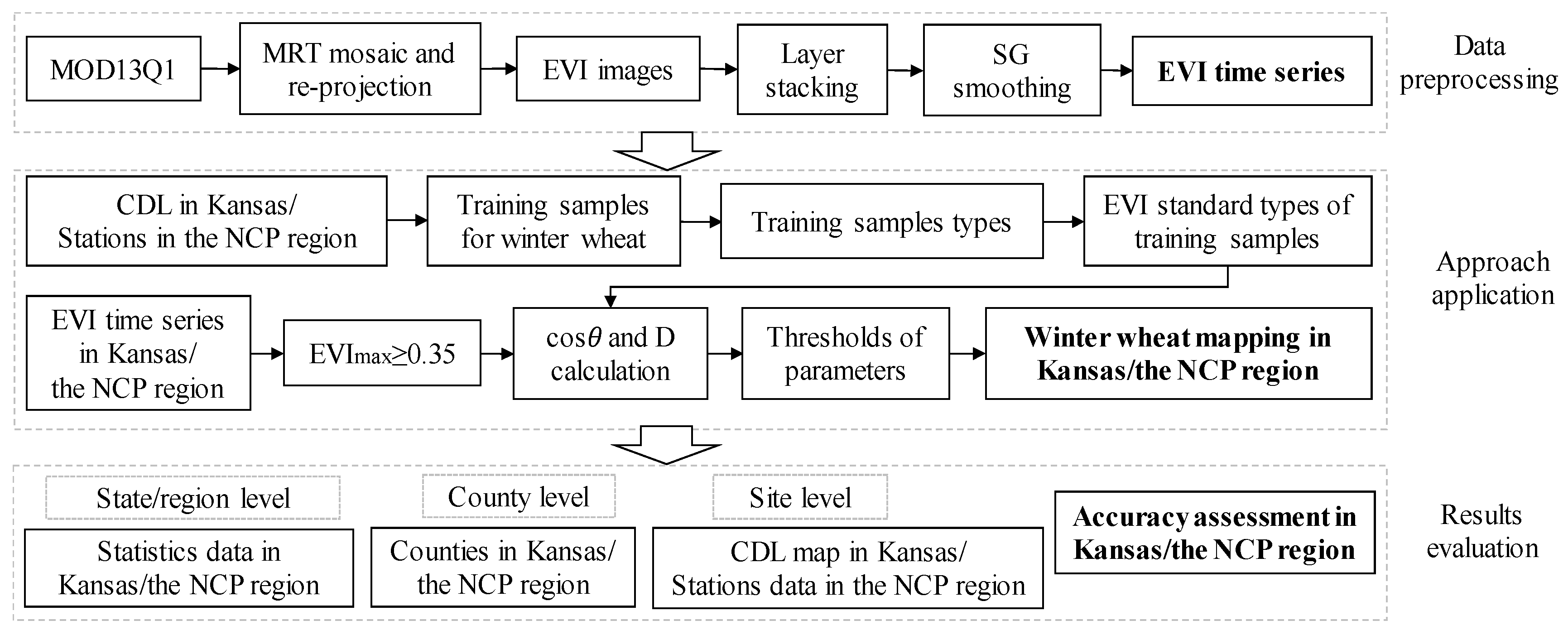
Statistical data at the administrative level were obtained to evaluate the mapped winter wheat areas in Kansas and the NCP. The 2017 winter wheat production areas at the county and state levels were collected from USDA-NASS website (https://quickstats.nass.usda.gov/) for Kansas. The 2017 winter wheat phenology information for Kansas was obtained from crop progress and condition reports at USDA-NASS website (https://www.nass.usda.gov/Charts_and_Maps/Crop_Progress_&_Condition). For the NCP, winter wheat planting statistics at the county level and provincial levels acquired from the Ministry of Agriculture of the People’s Republic of China (http://202.127.42.157/moazzys/nongqingxm.aspx/). Moreover, we collected phenological and locations information for the winter wheat crop from agrometeorological stations (http://data.cma.cn) across the NCP (Figure 1b).

3. Methods

The overall process diagram of this study is presented in Figure 2.

3.1. Winter Wheat Crop Calendars

The typical crop season length of winter wheat is about seven to nine months, including the prewinter growing period. For defining the time ranges of EVI time series, crop calendars acquired from USDA-NASS and agrometeorological stations for two study areas were used (Table 1). In Kansas, winter wheat is planted in mid-September, and 80% of winter wheat planting is done before mid-October. Harvest begins from mid-June, and 80% of wheat areas are harvested before late July in 2017. In the NCP, there are some differences in winter wheat phenology between the northern and the southern areas. Winter wheat is usually sown in October, but the earliest planting dates occur in late September. Winter wheat overwinters from late December to the next February and greens up in late February. In spring, winter wheat starts growing rapidly and is generally harvested in mid-June [46].

3.2. Data Preprocessing

The MODIS Reprojection Tool (MRT) (http://edcdaac.usgs.gov/datatools.asp) was used to generate EVI mosaics spanning three MODIS scenes (h09v05, h10v04, h10v05) for Kansas and five scenes (h26v04, h26v05, h27v04, h27v05, h28v05) for the NCP region for each 16-day composite images, respectively [36]. Based on the winter wheat phenology at two areas, EVI time series for the growing season for Kansas from mid-September 2016 to mid-July 2017 and for the NCP from late September 2011 to mid-June 2012 were used (Table 1). Images were reprojected to an Albers Equal-Area Conic projection by the nearest neighbor resampling method using the MRT [37]. Preprocessed data was then subset to the study boundaries (Kansas and the NCP), resulting in MODIS EVI time series stacks that cover the whole growth period of winter wheat for each study area.

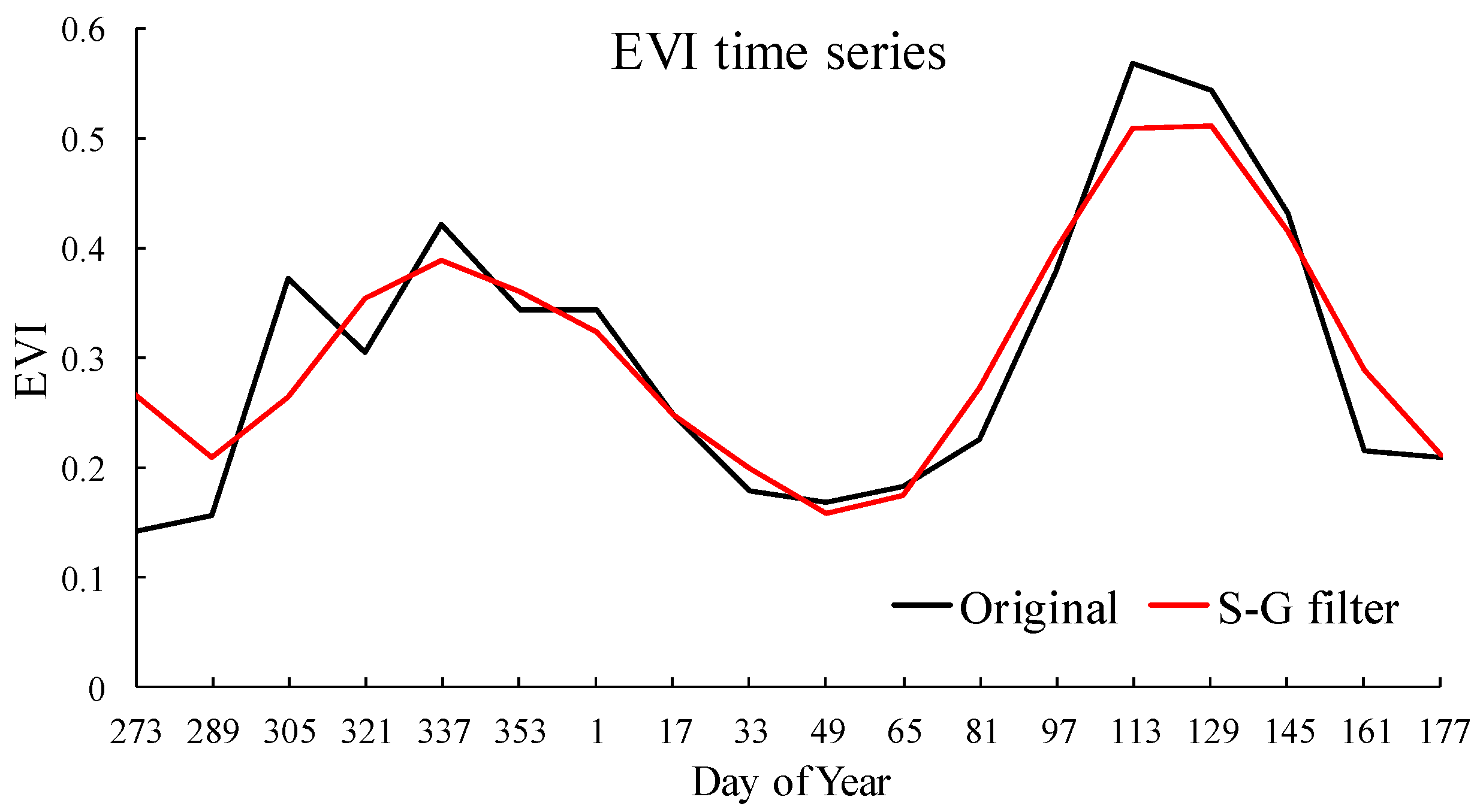
3.3. EVI Time Series Reconstruction by a Savitzky–Golay Filter

In this study, the Savitzky–Golay (S–G) filter was used to reconstruct the essential shape of the EVI time-series curve [47]. The S–G smoothing filtering is based on an asymmetric Gaussian function-fitting, also known as least squares or digital smoothing polynomial, which can be used to reduce the random noise from time series data [48,49]. This filter is widely used for the reconstruction of time series of remote sensing vegetation index [50]. Invalid points affected by external factors in the EVI time series will be eliminated during the S–G filtering course. We used ENVI software extensions to implement the S–G filter to perform an image-based time series filtering. The algorithm can be summarized as follows [47]:
g i = n = n L n = n R C n f i + n n
where f i represents the original EVI value in time-series; g i is the smoothed EVI value, which is the linear combination of C n and f i ; n is the width of the moving window to perform filtering, and n L and n R are the left and right edge of the signal component, respectively. Originally, if C n is a constant defined as C n = 1 / ( n L + n R + 1 ) , then the S–G filtering becomes a moving window smoothing. The idea of Savitzky–Golay method is to find filtering coefficients for C n that preserves higher moments. Therefore, in Eq. (2), the C n is not a constant but a polynomial fitting function. Then a least squares fit is solved ranging from n L to n R to obtain C n . For a specific dataset of a time-series in a moving window, we defined the fitting function as a quadratic polynomial for a specific f i [51,52]:
C n ( t ) = C 1 + C 2 t + C 3 t 2
where t corresponds to the day of the year in the EVI time series.
The S–G filtering is defined as a weighted-moving-average with weighting given as a polynomial of a certain degree. The filter can use any number of points for this weighted average. The returned coefficients, when applied to a signal, perform a polynomial least squares fit within the filter window. This polynomial is designed to preserve the high moments within the data and reduce the bias introduced by the filter. After the S–G filtering, the EVI time series were constructed for the two study areas (Figure 3) [47].

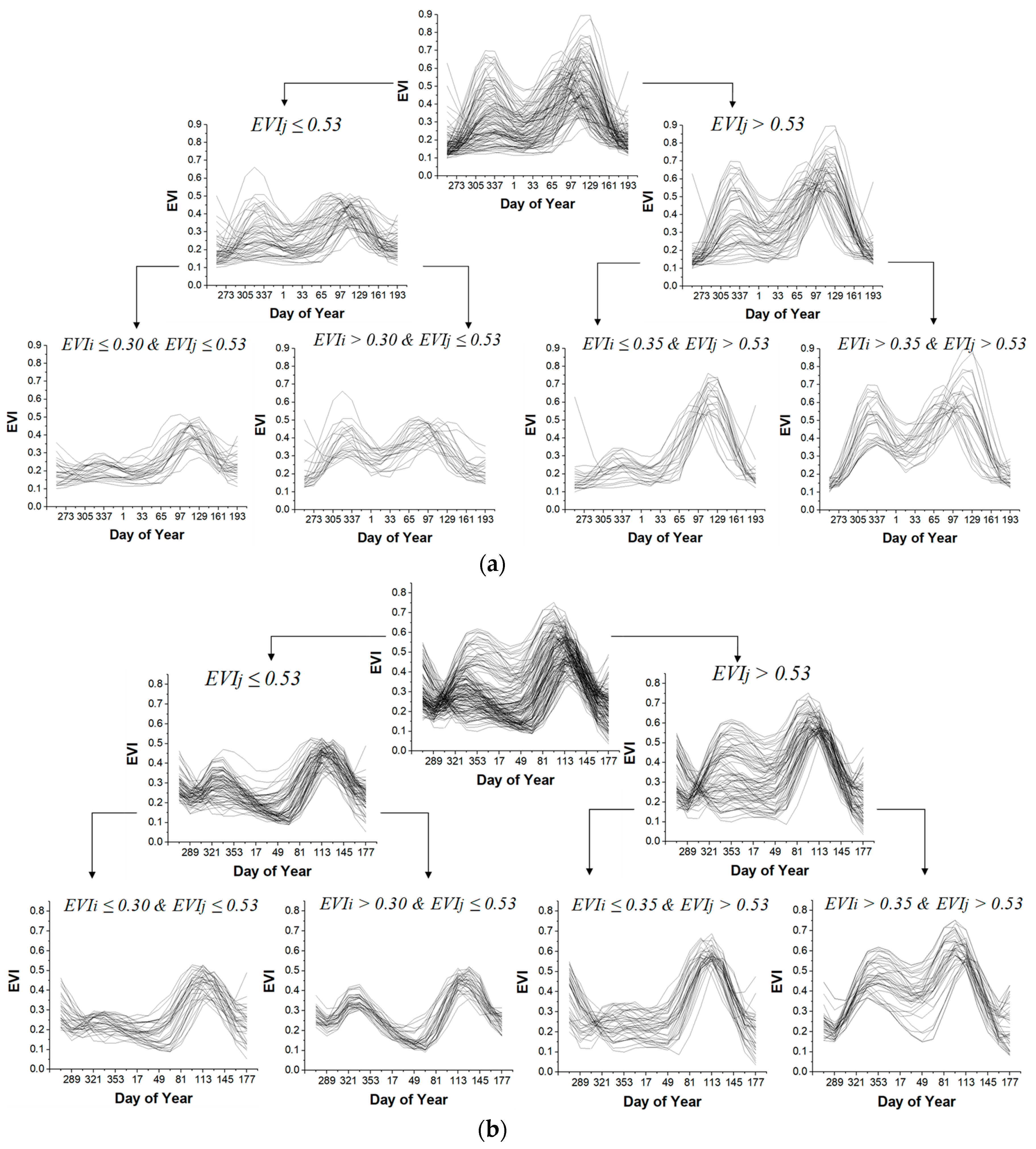
3.4. Extracting Training Samples Considering Intraclass Differences

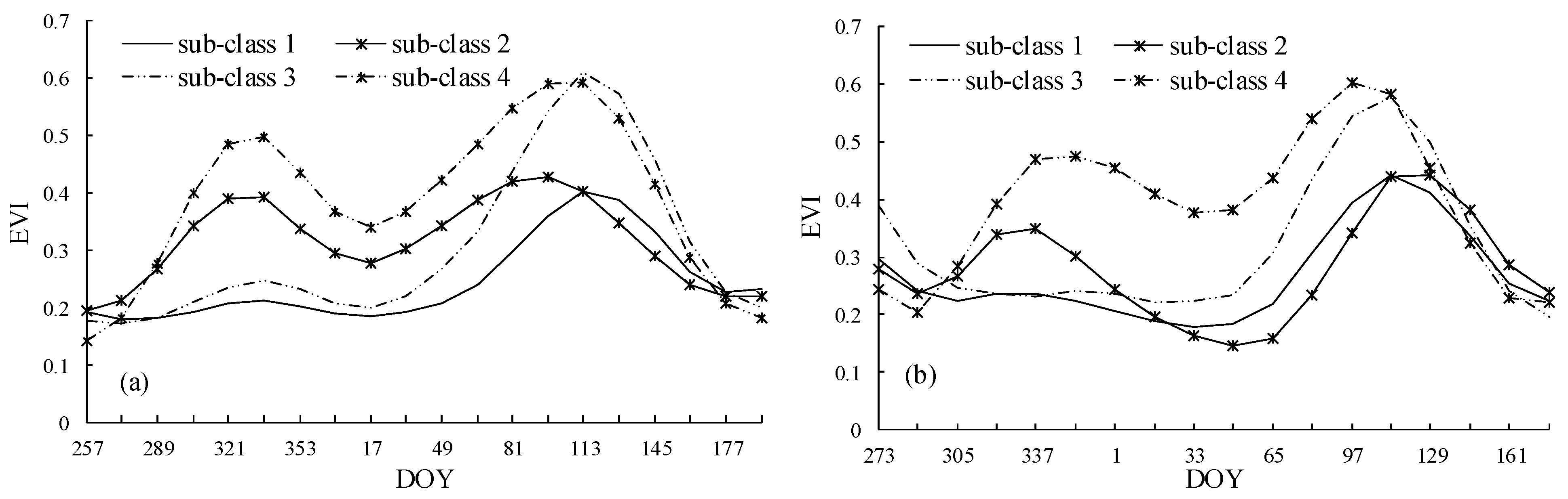
3.4.1. Generating Subclasses for the Two Study Areas

We randomly generated both training and validation sample locations for winter wheat and validation samples for no-winter wheat in the two study areas (Table 2). The 2017 CDL map was reprojected to Albers Equal-Area Conic projection and resampled to a 250 m spatial resolution by the nearest neighbor resampling method using ArcGIS 10.1 to correspond to the MODIS EVI time-series. The random samples for the winter wheat sites were obtained from the CDL map for Kansas and randomly divided into two sets, i.e., training samples and validation samples. Based on the Google Earth images, samples in the NCP were selected combined with the recorded agrometeorological stations, and all were randomly divided into training and validation samples.
Winter wheat has unique phenological characteristics different from other crops, which might be easier to identify and differentiate from other land features on remote sensing images. However, the EVI profiles may show different patterns for the same crop type as a result of intraclass variability resulting from regional variations in environmental conditions and management practices [8,14,17]. EVI curve morphology is affected by many factors, such as planting density, winter wheat varieties, climate factors, soil types, topographical conditions, etc.
In this study, the intraclass variability of winter wheat was fully considered in the process of building the subclass sets of training samples. The over-wintering period is an obvious physical feature of winter wheat fields, which divides the entire winter wheat growth period into two phases and results in double peaks in the EVI curve. In Figure 4, the EVI peak values before the wintering phase change from 0.1 to nearly 0.65 and the second peak values vary from about 0.35 to around 0.85. The wide differences at each EVI peak exhibit obvious winter wheat intraclass variability, which was adopted as the unique features to extract subclass training samples. Selecting these two EVI peaks as the segmentation points to divide subclasses is more appropriate than other points.
The training samples were randomly selected across the study area, which represent the winter wheat crop for the whole study area. Figure 4 shows that the EVI values at two peaks were distributed roughly even from low to high. Taking the medians of EVI peak values as the thresholds can divide the total training samples into each subclass with similar amounts. The median of second EVI peak values was 0.53, which was used for dividing all training samples to two first-level subclasses. The thresholds 0.3 and 0.35 were the medians of two first-level subclasses and subdivided training sets into four second-level subclasses. Thus, the segmentation thresholds of four subclasses in two study areas are shown in Table 3.

3.4.2. Calculating the Separability of Subclasses Using Jeffries–Matusita (JM) Distance

In combination with the Jeffries–Matusita (JM) Distance, we provided a measure of the overall separability between four subclasses and other land cover types [53]. JM distance has been demonstrated to be an effective metric for evaluating the separability of training samples in remote sensing-based classification [14,54]. We examined the JM distances using the EVI time series for each pair of types (Table 4) to evaluate the feasibility of segmentation thresholds of each subclass.
To calculate the JM distance, we randomly selected six main land cover types (not including winter wheat) as the training sets from CDL maps in Kansas. Combining with Google Earth images and the GlobeLand30 dataset (http://www.globeland30.org/GLC30Download/index.aspx), five major land cover types were also selected in the NCP. Land cover types obtained for calculating JM distances for two study areas are shown in Table 4.
The calculation of JM distance between two types is [14]:
JM ( C j , C k ) = x ( p ( x | C j ) p ( x | C k ) ) 2 d x
where, x represents a span of EVI time series values, and C j and C k are the two types under consideration. Under normality assumptions, Equation (3) reduces to JM = 2 ( 1 e B ) , where
B = 1 8 D 2 + 1 2   ln ( | | j + k | 2 | / | j |   | k | )
D 2 = ( μ j μ k ) T ( j + k 2 ) 1 ( μ j μ k )
where, μ j and μ k correspond to type-specific, expected EVI values, and j and k are unbiased estimates for the type-specific covariance matrices. The range of JM distance distribution is between 0 to 2 . Larger JM distances indicate more distinct distributions between two types, which favors successful type identification.

3.5. The Improved Approach to Winter Wheat Detection

3.5.1. Calculating Standard Vectors for Two Study Areas

Considering the EVI time series as n-dimensional vectors, the average of each subclass training dataset was calculated as the standard vector. We calculated the standard vector in each subclass as:
V s = ( i = 0 n 1 v 0 i ,    i = 1 n 1 v 1 i ,       i = n 1 n 1 v ( n 1 ) ( n 1 ) n
where n is the dimension of EVI time series, i = n − 1.
Based on the above equation, we calculated four standard vectors (e.g., subclass 1, subclass 2, subclass 3, and subclass 4) for the two study areas, respectively. The differences between four standard vectors illustrating the intraclass variability of winter wheat are shown in Figure 5.

3.5.2. Calculating Two Parameters

Based on the standard vector calculated for each subclass (Figure 5), two parameters c o s θ and D were generated for both study areas in ENVI-IDL environment. Two parameters (angle and distance) were calculated between the total EVI time series for the whole study areas and each standard vector, respectively, as [55,56,57,58] (7):
V = ( v 0 , v 1 , v 2 , v i 1 ) , V s = ( v s 0 , v s 1 , v s 2 , v s ( i 1 ) ) { a n g l e :   cos θ   =   V V s V 2 V s 2 d i s t a n c e :   D   =   ( V V s ) 2
where V is EVI time series vector, V s is standard vector, i = n − 1, n is the dimension of the vector, θ and D are the angle and distance between the EVI time series vectors and four standard vectors, respectively.
We generated eight parameters, including four angle parameters ( e . g . ,   c o s θ 1 ,   c o s θ 2 ,   c o s θ 3 , and c o s θ 4 ), and four distance parameters ( e . g . , D 1 ,   D 2 ,   D 3 , and D 4 ) were then generated for each study area. Parameters with the same number label were calculated from the same standard vector. For example, the parameter c o s θ 1 and D 1 were computed based on the standard vector extracting from subclass 1.

3.5.3. The Sensitivity Tests to Thresholds of Parameters

We calculated the ranges of the angles and distances between the standard vectors and relative subtraining samples based on Equation (7) to determine the thresholds. We also performed a sensitivity study to test the effects of thresholds on the mapping results. Eight tests were examined for each study area based on the same training samples (Table 5). The optimum thresholds of four subclasses were determined by the evaluation of the sensitivity test.

3.5.4. The Algorithm to Extract Winter Wheat Mapping

Nonvegetated areas were masked out based on the smoothed EVI time series. According to the training samples, maximum EVI values of winter wheat were determined to be greater than 0.35 at both study areas [59,60]. Four submaps were extracted based on individual thresholds of the four subclasses. We integrated all four submaps and areas under the mask using Equation (8) to generate the winter wheat maps in both study areas.
{ E V I m a x 0.35 { c o s θ 1   a 1 D 1   d 1 { c o s θ 2   a 2 D 2   d 2 { c o s θ 3   a 3 D 3   d 3 { c o s θ 4   a 4 D 4   d 4
where thresholds a 1 ~ a 4 , d 1 ~ d 4 were determined according to subclass training samples.

3.6. Statistical Analysis

We evaluated our results using the statistical data at the state/regional level for the two study areas. Percentage Error (PE) was used to quantify the differences of winter wheat mapping areas between the statistical data and our results as:
PE = | O b s e r v e d E s t i m a t e d | O b s e r v e d × 100 %
The accuracy was calculated as:
Accuracy = 100 % PE
where O b s e r v e d and E s t i m a t e d represent the statistical data and results in this study.
Root mean square error (RMSE) and coefficient of determination (R2) were used to compare the statistical data and estimated winter wheat areas at the county level for the two study areas as:
R 2 = i = 1 n ( x i x ¯ ) 2 ( y i y ¯ ) 2 i = 1 n ( x i x ¯ ) 2 i = 1 n ( y i y ¯ ) 2
RMSE = 1 n i = 1 n ( y i x i ) 2
where n represents the number of counties; y i and x i are the statistical and estimated data, respectively.
For the site-level evaluation, the confusion matrix was created, including the overall accuracy (OA), Kappa coefficient (KAPPA), producer’s accuracy (PA), and user’s accuracy (UA). The overall accuracy (Equation 13) represents the percentage of validation samples that are correctly identified [61]. The Kappa coefficient measures the agreement between observations and prediction results. Kappa coefficient value of 1 represents perfect agreement, while a value of 0 represents no agreement. (the definitions of producer’s accuracy and user’s accuracy have been explained in Section 2.2.2) Overall accuracy and the Kappa coefficient were computed as following [62]:
Overall   Accuracy = T o t a l   n u m b e r   o f   c o r r e c t   e s t i m a i t o n s T o t a l   n u m b e r   o f   d a t a s e t
KAPPA = N i = 1 r x i i i = 1 r ( x i + × x + i ) N 2 i = 1 r ( x i + × x + i )
where r is the number of rows in the matrix, x i i is the number of observations in row i and column i , x i + and x + i are the marginal totals of row i and column i , respectively, and N is the total number of observations.

3.7. Landscape Metrics Analysis

Remote sensing-based crop mapping accuracy achieved based on moderate resolution data is related to the spatial heterogeneity of the observed cropland [28]. In this study, we quantified the relationship between landscape metrics and winter wheat mapping accuracy. We reclassified all land cover types into two classes (winter wheat and others) using ArcGIS 10.1 based on the CDL dataset for Kansas. We then generated individual maps for 75 counties from the reclassified map and calculated the percentage errors of our results based on the CDL dataset using Equation (5). Two landscape fragmentation metrics were calculated in FRAGSTATS version 4.2 to characterize the landscape structures for these 75 counties. As a metric of spatial configuration, the fragmentation index (FRG) was calculated based on the number of patches and pixels of a given class [63]. Percentage of the landscape (PLAND) is the other class metric, which is related to landscape fragmentation because it measures the fraction or proportional abundance of a particular patch type [64]. The relationships between landscape metrics and extraction errors of our improved approach at the county level were analyzed using a linear regression model. The metrics were calculated as follows:
FRG = ( n 1 ) ( m 1 )
where n is the number of winter wheat patches, and m is the number of pixels composing the patches of winter wheat.
P i = j = 1 n i a i j A
PLAND = P i × 100 %
where i = 1 , , s . s is the total number of patch types, a i j is an area of the j t h patch that belongs to cover type i , A is the total area of the landscape.

3.8. Other Methods without Intraclass Variability

3.8.1. The Approach Integrated the Angles and Distances without Considering Intraclass Variability

To validate the importance of intraclass variability on winter wheat mapping accuracy, we conducted a comparative experiment to map winter wheat for both study areas using the same training samples. The same approach described above was used (Section 3.5) but without considering intraclass variability.
In the comparative experiment, we did not divide subclasses. Based on Equation (6), we calculated the standard vector using all training samples for both study areas, respectively. Equation (7) in Section 3.5.2 was used for generating two parameters ( c o s θ and D ). Equation (8) was reduced to the following:
{ EVI max 0.35 { c o s θ   a D   d
where thresholds a and d were determined according to all training samples.

3.8.2. The Traditional Classification Methods without Considering Intraclass Variability

To further compare the results of our approach to existing methods, we generated winter wheat maps using three traditional classification methods including the maximum likelihood (MLC) [23], support vector machine (SVM) [25] and artificial neural network (ANN) [24]. Based on the training samples shown in Table 4, we conducted winter wheat mapping using these three traditional classification methods for two study areas, respectively. The accuracies were evaluated using the same validation samples.

4. Results

4.1. Separability Comparisons Based on the Jeffries–Matusita (JM) Distance

The separabilities between each winter wheat subclass and other land cover types in the time-series EVI data were investigated using the JM distance in Kansas and the NCP (Table 6). The JM distances among four subclasses are higher than 1.92 in both study areas, indicating that four subclasses are separable under the determined segmentation in this study. In addition, all four subclasses of winter wheat had JM distances over 1.98 when compared with each of the other land cover types.

4.2. Sensitivity Study for Testing Thresholds of Parameters

Accuracies based on CDL maps in Kansas and statistical data in the NCP (in Section 3.6) were used to evaluate the effects of the thresholds of parameters on mapping accuracies in two study areas (Table 7). The thresholds with the best performance (Test 6) for each study area were selected as the optimum parameters. Thus, the winter wheat mapping distribution was generated based on the optimum parameters in both study areas.

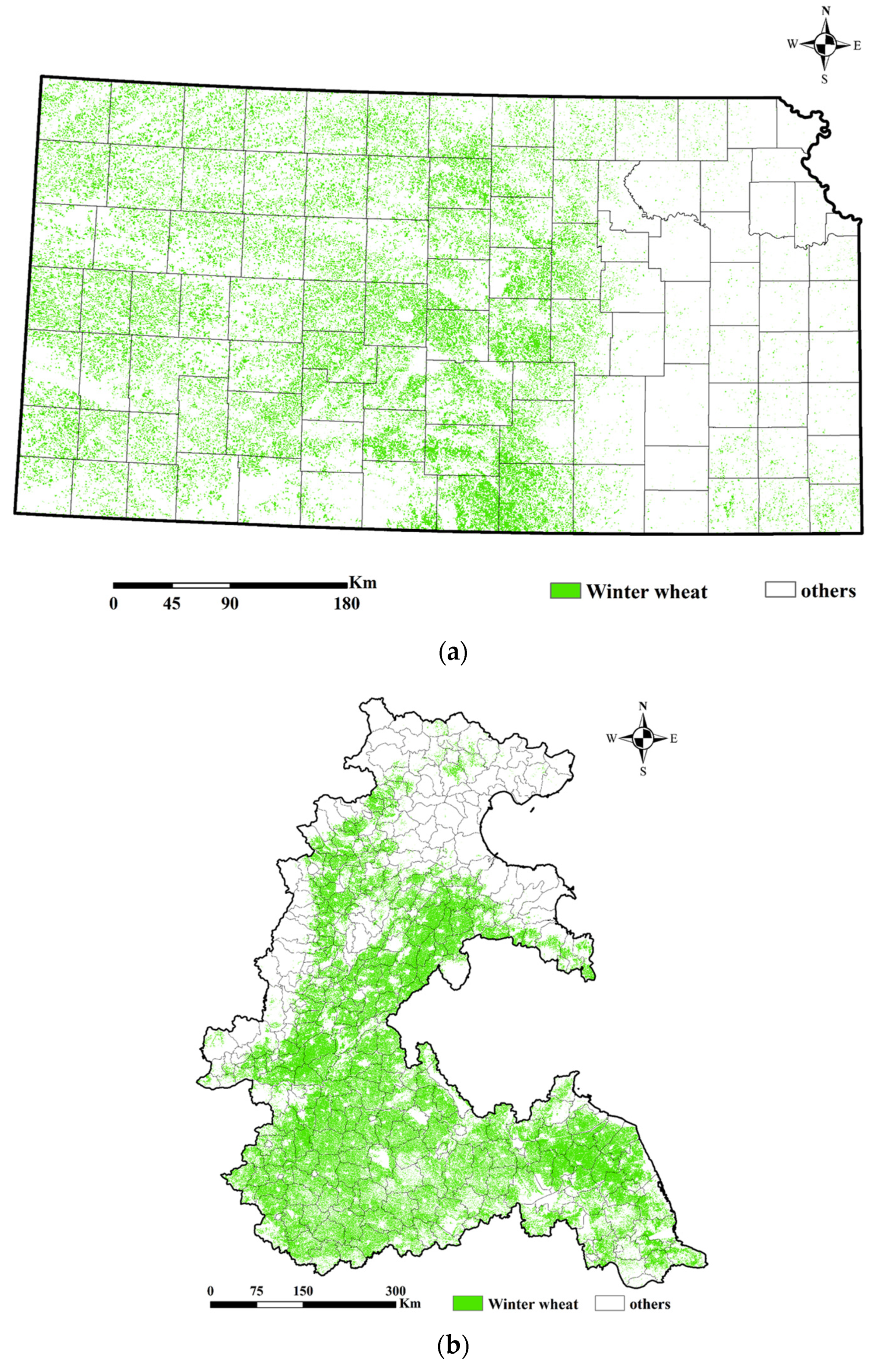
4.3. Winter Wheat Distribution Mapping for Kansas and the NCP

We used the optimal parameter values (Table 5) from the sensitivity study (Test 6) to map winter wheat in Kansas and the NCP (Figure 6). For Kansas, the spatial distribution of winter wheat (Figure 6a) is consistent with that derived from the CDL maps developed based on the Landsat images (Figure 1a). Winter wheat fields mainly concentrate in the middle and west area and distribute sporadically in the southeast of Kansas. There are only minor areas of winter wheat cultivation in the Northeast. For the NCP, winter wheat is the predominant crop type in the summer growing season, accounting for more than 90% of the farmland in this area [65]. The primary region of winter wheat cultivation is in south-central Hebei province, almost the entire Henan province, the west and southwest of Shandong province, and the north of Anhui and Jiangsu provinces (Figure 6b).

4.4. Evaluation of Winter Wheat Maps at the State/Regional Level

For evaluating the winter wheat distribution maps, we calculated percentage errors and accuracies for Kansas and the NCP (Table 8). The evaluation results showed favorable performances in the two areas with percentage errors lower than 10%, i.e., the accuracies were both higher than 90% as compared with the statistical data at the state/regional scale. Specifically, the winter wheat mapping accuracy in Kansas (95.1%) was slightly higher (2.2%) than that in the NCP (92.9%). Moreover, the accuracy at the state level in this study was 99.2% compared with the Landsat-derived CDL maps for Kansas [66,67]. The estimated winter wheat areas were slightly larger than those from statistical data partially because the farmland’s fragmentation resulted in some discrete pixels of other land types being assigned to winter wheat, which cannot be detected at a 250 m spatial resolution [18].

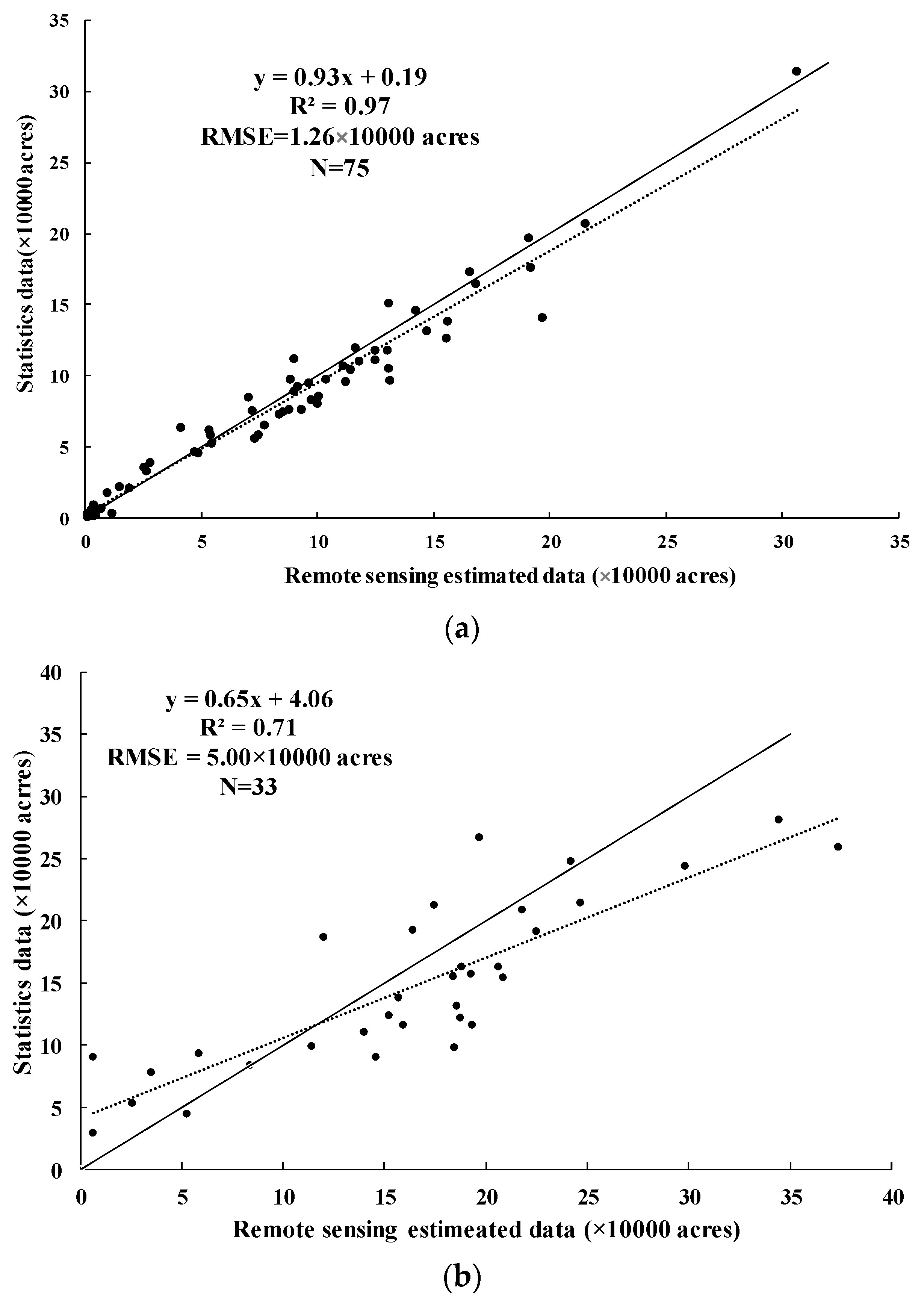
4.5. Evaluation of Winter Wheat Maps at the County Level

We compared our winter wheat distribution maps in 2017 for Kansas and 2012 for the NCP against the ground reference data at the county level (75 counties for Kansas and 33 counties for the NCP). The results showed that our estimated winter wheat areas are in good agreement with that of the county-level for Kansas (Figure 7a), with a coefficient of determination (R2) as high as 0.97. For the NCP, our results showed an R2 of 0.71 as compared with census based on 33 counties. The RMSE value in Kansas was about one-fourth of that in the NCP, illustrating that the winter wheat mapping approach performed better in Kansas than in the NCP.

4.6. Evaluation of Winter Wheat Maps at the Site Level

We further evaluated our winter wheat maps at the site level based on randomly selected sample units derived from the CDL for Kansas and agrometeorological stations for the NCP [62,68]. The evaluation samples were selected across the entire study area to ensure they reflected diverse environmental conditions and management practices [18]. These samples were independent of the training data [69].
Confusion matrix suggested that the overall accuracies are 90.3% and 85.0% for Kansas and the NCP, respectively. The Kappa coefficient was 0.81 for Kansas, 0.11 higher than that for the NCP. The producer’s and user’s accuracy in Kansas were 87% and 93.2%, respectively, slightly higher than those for the NCP (Table 9).

4.7. Correlation between Landscape Metrics and Winter Wheat Mapping Accuracy

For estimating the effects of landscape fragmentation on the mapping accuracy, we calculated two class-scale fragmentation metrics (FRG and PLAND) for 75 counties based on the CDL map in Kansas. We divided the calculated landscape metrics into five categories according to the fragmentation levels and examined the correlations between the metrics and the percentage errors of our winter wheat maps at the county level (Table 10). Our analysis showed a strong positive correlation (r = 0.99) between the winter wheat FRG and the percentage errors, indicating a better performance for our approach in areas with lower fragmentation. Similarly, higher PLAND values correspond to higher mapping accuracies. When the PLAND value was less than 1%, the average percentage error reaches 59.4%; when the PLAND values were larger than 20%, the average percentage errors were lower than 10%.

4.8. Comparisons with Other Methods without Considering Intraclass Variability

Table 11 shows the overall accuracies and Kappa coefficients of winter wheat mapping using methods with and without considering intraclass variability in the two study areas. The overall accuracies were calculated based on the same validation samples using the confusion matrix in each study area. Similar performance was detected by SVM and ANN methods in both study areas. The MLC method showed the lowest overall accuracy (73% in Kansas). In the NCP, overall accuracy is lower than 70% using the integrated angles and distances of the EVI time series without considering intraclass variability. The improved approach presented in this study performed well, with overall accuracies over 85% in both study areas.
As a result, the overall accuracies in Kansas and the NCP have been improved by 17% and 15% with Kappa coefficients increased by 0.35 and 0.38, respectively, using the improved approach. The comparisons among methods with and without considering the intraclass variability reveal that our approach can effectively improve winter wheat mapping accuracy.

5. Discussion

5.1. Winter Wheat Mapping Approach Considering Intraclass Variability

A range of crop type mapping approaches has been developed in previous studies based on the similarities of the same class and dissimilarities of different categories [12,14,70,71]. However, few of them have included intraclass variability caused by the differences in environmental status and management practices [22]. Characterizing the intraclass variability (e.g., crop phenology, growth conditions, field management) over large areas remains a big challenge [8,14,17]. The improved quality of remote sensing images (spectral, spatial, and temporal resolutions) led to an increase not only in the interclass variability but also in the intraclass variability [31], which might compromise the mapping accuracy when the intraclass variability is more apparent than interclass differences. Therefore, considering intraclass variability is necessary for individual crop type identification.
Although high-resolution remote sensing imagery provides the possibility to identify the differences within a class [12], it is still difficult to characterize such factor-driven differences using the traditional crop type mapping methods [31,71]. In our study, the intraclass variability was considered for winter wheat areas mapping based on MODIS EVI time series data. We found wide differences among all MODIS EVI time series curves of winter wheat samples at both study areas (Figure 4). Two peaks of the EVI time series curve were used to express the intraclass discrepancy of training samples for introducing intraclass variability into the mapping approach. We divided all training samples into four subclasses based on the differences of EVI values at the two peaks, and then introduced two parameters (the angle and distance of multidimensional vector) to describe the characteristics of subclasses. JM distances were evaluated between each subclass of winter wheat and other land cover types, which showed that all subclasses were highly distinguishable from others. The evaluation of results considering intraclass variability suggested that the two parameters were important for characterizing the intraclass variability. Our mapping accuracies of winter wheat were both over 92% (Table 10) compared with statistical data at the regional/state level.
We also compared our results with methods without considering the intraclass variability of winter wheat. Considering intraclass variability improved the winter wheat mapping accuracies by 17% in Kansas and 15% in the NCP, respectively. Our results demonstrated the importance of introducing subclass training samples into crop mapping. This study also showed that the MODIS 250 m EVI data could serve as a powerful tool to assess the intraclass variability for crop type identification [14].

5.2. Factors Influencing the Accuracy of Winter Wheat Maps

The differences in mapping accuracies at two study areas might be attributed to the specific conditions of these two study areas. Compared with Kansas, winter wheat fields in the NCP are difficult to identify partially due to the relatively small field sizes [20,72], irregular patterns of crop system [65], and relatively fewer training samples. Same as most of the cropland areas in China, croplands in the NCP are split into many small parcels allocated to households, and farmers have their freedom on planting under private land use rights [73]. Our landscape metrics analysis demonstrated the impacts of cropland fragmentation on the mapping accuracies [20]. Higher land fragmentation level generally corresponds to lower winter wheat mapping accuracies, which may partly explain the relatively higher mapping accuracies in Kansas. Moreover, due to the specific land allocation policy in China, croplands in the same region might be dominated by different cropping patterns or growing times, which shows a high degree of fragmentation on remote sensing images and makes it more complicated for crop mapping. This also suggested that the MODIS EVI 250 m data has a significant advantage for crop mapping in intensively managed landscapes with a low degree of fragmentation [70]. In the U.S. Central Great Plains, the field sizes are generally larger than 30 ha, which spatially corresponds to five or more 250 m pixels [18]. In addition, the lack of training samples in the NCP might be another factor influencing the mapping accuracy. The CDL map at 30 m spatial resolution provides a useful dataset for generating enough effective training samples for crop mapping. In China, the existing crop mapping products are very limited for choosing training samples. In this study, training samples collected from the agrometeorological stations have coarser spatial resolution than those extracted from the CDL map for Kansas. The mapping accuracy in the NCP could be improved as more ground information or more high-resolution crop distribution maps are available.

5.3. Comparison with Other Studies

Currently, intraclass variability has not been well considered in crop mapping. Few efforts have been made to use areas segmentation to analyze and reduce intraclass differences. For example, Wardlow et al. calculated and compared average VI profiles for each crop type at the ASD–USDA NASS Agricultural Statistics District level to assess their intraclass regional variations based on MODIS data [14]. They detected that the regional intraclass variations reflect the state’s climate and planting date gradient across Kansas. In another study [18], considering the notable regional differences in crop area and locations, Wardlow et al. presented a hierarchical crop mapping approach using a decision tree classifier and identified individual crop types including winter wheat based on the crop/noncrop maps with accuracies ranging from 84% to 94%. Different from Wardlow et al. [18], our approach is capable of detecting winter wheat from MODIS products without the need for a cropland-based map or a large number of field sites as inputs, and therefore has potential to be applied over large areas where crop maps and site-level observations are scarce. Using MODIS 250 m data, Massey et al. divided the U.S. cropland areas into 299 subzones for reducing the intraclass variability and classified wheat-barley with 84.2% and 74.5% in producer’s accuracy and user’s accuracy, respectively [33]. In this study, we divided the training samples into four subclasses and obtained higher producer’s accuracy (87.0%) and user’s accuracy (93.2%).
For the NCP, a large number of studies have focused on winter wheat mapping. For example, Pan et al. constructed a Crop Proportion Phenology Index (CPPI) to estimate the winter wheat area using MODIS EVI time series and achieved accuracies with R2 varied from 0.5 to 0.9 and RMSE ranging from 5% to 20% compared with the Landsat-based maps [20]. Their study highlighted the importance of the representativeness, quality, and quantity of samples for the mapping accuracies at a large scale because the agricultural areas may have diverse planting structures, climate conditions, and topographies. Notably, this study also highlighted that dividing the large study area into different subregions based on various factors and selecting different samples in each subregion would be helpful and need to be tested in future work [20]. Tao et al. also performed winter wheat mapping on the NCP and showed the accuracies in seven provinces to range from 87 to 96% compared with statistical data [72]. In this study, our mapping accuracy for the NCP region was 92.9%, and the R2 was 0.71 compared with the county-level census, falling within the range reported in previous studies. Our accuracies were calculated based on the entire NCP region (vs. seven provinces in Tao et al. [60]) or county-level census (33 counties vs. samples from the Landsat-based maps in Pan et al. [20]). Moreover, our study introduced the subclasses as training samples for winter wheat mapping, combined with two parameters, i.e., the angles and distances based on EVI time series data, which represents an advanced approach compared to previous studies. The introduction of the angles and distances allowed us to capture the unique phenological features of winter wheat and achieved a better mapping performance.

5.4. Uncertainty Analysis and Future Needs

In this study, we demonstrated the advantages of introducing intraclass variability to winter wheat mapping. However, some uncertainties should be addressed in the future. First, the parameter thresholds used for winter wheat mapping are different for Kansas and the NCP region, and are related to crop field management, the degree of cropland fragment, crop condition, climate, etc. These factors should be quantified in the future to examine how they affect the setting of thresholds under different conditions. Second, we envision that our approach has the potential to be well suited for relatively wide agroclimatic regions. Further efforts are needed to evaluate the feasibility in other winter wheat areas where the environmental conditions may be substantially different from those in our two study areas. Third, more work is needed for extending this approach to other crop types such as rice. In addition, although the 250 m MODIS data used can be applied to agricultural areas where winter wheat is the dominant crop, finer resolution satellite data such as Sentinel-2 MSI are needed to provide imagery with a high spatial resolution for crop mapping over regions where highly fragmented crop fields occur. As more field observations and high-resolution images become available, the performance of this approach could be further enhanced in future research.

6. Conclusions

In this study, we presented an improved approach for winter wheat mapping based on the MODIS EVI time series, in which intraclass variability effects were considered. To the best of our knowledge, this study offered the first attempt to introduce the subclass training samples for interpreting the intraclass variability based on the angles and distances of EVI time series in winter wheat area mapping. Comparison with other methods showed that our approach considering intraclass variability improved the winter wheat mapping accuracies by 17% in Kansas and 15% in the NCP, respectively. The mapping results compared well with those from multiscale ground information at the two areas of interest. Further analysis demonstrated that the mapping accuracy could be significantly affected by landscape fragmentation. This study provides a new perspective for decreasing the influences of intraclass variability in cropland mapping. Our winter wheat identification algorithm can be applied to other agricultural areas where ground information is available for parametrization and validation. In addition, the derived winter wheat maps can be used to drive crop or ecosystem models for investigating regional variations in crop productivity and associated environmental consequences.

Author Contributions

Y.Y., B.T., and W.R. conceived and designed the research. Y.Y. performed the research, analyzed, and interpreted the data. B.T. and W.R. were responsible for the research analysis. Y.Y. and B.T. contributed to the writing of the manuscript. W.R., Q.T., D.P.Z., B.E.M., and Z.S. reviewed and revised the manuscript.

Funding

This research was funded by the National Institute of Food and Agriculture, U.S. Department of Agriculture (NIFA-USDA Hatch project), grant number 2352437000.

Acknowledgments

We thank four anonymous reviewers and the editor for comments that improved this manuscript. We acknowledge the use of the MODIS data from the Land Processes Distributed Active Archive Center (LPDAAC) (http://lpdaac.usgs.gov/) and the Cropland Data Layer (CDL) maps from CropScape (http://nassgeodata.gmu.edu/CropScape/).

Conflicts of Interest

The authors declare no conflict of interest.

References

  1. Yearbook, F.S. Asia and the Pacific, Food and Agriculture; FAO: Budapest, Hungary, 2014. [Google Scholar]
  2. Lobell, D.B.; Sibley, A.; Ortiz-Monasterio, J.I. Extreme heat effects on wheat senescence in India. Nat. Clim. Chang. 2012, 2, 186. [Google Scholar] [CrossRef]
  3. Ortiz, R.; Sayre, K.D.; Govaerts, B.; Gupta, R.; Subbarao, G.V.; Ban, T.; Hodson, D.; Dixon, J.; Ortiz-Monasterio, J.I.; Reynolds, M. Climate change: Can wheat beat the heat? Agric. Ecosyst. Environ. 2008, 126, 46–58. [Google Scholar] [CrossRef]
  4. Becker-Reshef, I.; Vermote, E.; Lindeman, M.; Justice, C. A generalized regression-based model for forecasting winter wheat yields in Kansas and Ukraine using MODIS data. Remote Sens. Environ. 2010, 114, 1312–1323. [Google Scholar] [CrossRef]
  5. Lobell, D.B.; Field, C.B. Global scale climate–crop yield relationships and the impacts of recent warming. Environ. Res. Lett. 2007, 2, 014002. [Google Scholar] [CrossRef]
  6. Tilman, D.; Balzer, C.; Hill, J.; Befort, B.L. Global food demand and the sustainable intensification. Proc. Natl. Acad. Sci. USA 2011, 108, 20260–20264. [Google Scholar] [CrossRef]
  7. Godfray, H.C.J.; Beddington, J.R.; Crute, I.R.; Haddad, L.; Lawrence, D.; Muir, J.F.; Toulmin, C. Food security: The challenge of feeding 9 billion people. Science 2010, 327, 812–818. [Google Scholar] [CrossRef] [PubMed]
  8. Qiu, B.; Luo, Y.; Tang, H.; Chen, C.; Lu, D.; Huang, H.; Chen, Y.; Chen, N.; Xu, W. Winter wheat mapping combining variations before and after estimated heading dates. ISPRS J. Photogramm. 2017, 123, 35–46. [Google Scholar] [CrossRef]
  9. Zheng, Y.; Zhang, M.; Zhang, X.; Zeng, H.; Wu, B. Mapping winter wheat biomass and yield using Time series data blended from PROBA-V 100- and 300-m S1 products. Remote Sens. 2016, 8, 824. [Google Scholar] [CrossRef]
  10. Wu, D.; Yu, Q.; Lu, C.; Hengsdijk, H. Quantifying production potentials of winter wheat in the North China Plain. Eur. J. Agron. 2006, 24, 226–235. [Google Scholar] [CrossRef]
  11. Siachalou, S.; Mallinis, G.; Tsakiri-Strati, M. A Hidden Markov Models Approach for Crop Classification: Linking Crop Phenology to Time Series of MultiSensor Remote Sensing Data. Remote Sens. 2015, 7, 3633–3650. [Google Scholar] [CrossRef]
  12. Atzberger, C. Advances in Remote Sensing of Agriculture: Context Description, Existing Operational Monitoring Systems and Major Information Needs. Remote Sens. 2013, 5, 949–981. [Google Scholar] [CrossRef]
  13. Xiao, X.; Boles, S.; Liu, J.; Zhuang, D.; Frolking, S.; Li, C.; Salas, W.; Moore, B., III. Mapping paddy rice agriculture in southern China using multitemporal MODIS images. Remote Sens. Environ. 2005, 95, 480–492. [Google Scholar] [CrossRef]
  14. Wardlow, B.; Egbert, S.; Kastens, J. Analysis of time-series MODIS 250 m vegetation index data for crop classification in the U.S. Central Great Plains. Remote Sens. Environ. 2007, 108, 290–310. [Google Scholar]
  15. Potgieter, A.B.; Apan, A.; Hammer, G.; Dunn, P. Early-season crop area estimates for winter crops in NE Australia using MODIS satellite imagery. ISPRS J. Photogramm. Remote Sens. 2010, 65, 380–387. [Google Scholar] [CrossRef]
  16. Justice, C.O.; Vermote, E.; Townshend, J.R.; Defries, R.; Roy, D.P.; Hall, D.K.; Lucht, W. The Moderate Resolution Imaging Spectroradiometer (MODIS): Land remote sensing for global change research. IEEE Trans. Geosci. Remote Sens. 1998, 36, 1228–1249. [Google Scholar] [CrossRef]
  17. Lunetta, R.S.; Shao, Y.; Ediriwickrema, J.; Lyon, J.G. Monitoring agricultural cropping patterns across the Laurentian Great Lakes Basin using MODIS-NDVI data. Int. J. Appl. Earth Obs. 2010, 12, 81–88. [Google Scholar] [CrossRef]
  18. Wardlow, B.D.; Egbert, S.L. Large-area crop mapping using time-series MODIS 250 m NDVI data: An assessment for the U.S. Central Great Plains. Remote Sens. Environ. 2008, 112, 1096–1116. [Google Scholar] [CrossRef]
  19. Sun, H.; Xu, A.; Lin, H.; Zhang, L.; Mei, Y. Winter wheat mapping using temporal signatures of MODIS vegetation index data. Int. J. Remote Sens. 2012, 33, 5026–5042. [Google Scholar] [CrossRef]
  20. Pan, Y.; Li, L.; Zhang, J.; Liang, S.; Zhu, X.; Sulla-Menashe, D. Winter wheat area estimation from MODIS-EVI time series data using the Crop Proportion Phenology Index. Remote Sens. Environ. 2012, 119, 232–242. [Google Scholar] [CrossRef]
  21. Song, Y.; Wang, J. Mapping Winter Wheat Planting Area and Monitoring Its Phenology Using Sentinel-1 Backscatter Time Series. Remote Sens. 2019, 11, 449. [Google Scholar] [CrossRef]
  22. Yang, C.; Everitt, J.H.; Murden, D. Evaluating high resolution SPOT 5 satellite imagery for crop identification. Compt. Electron. Agric. 2011, 75, 347–354. [Google Scholar] [CrossRef]
  23. Booth, D.J.; Oldfield, R.B. A comparison of classification algorithms in terms of speed and accuracy after the application of a post-classification modal filter. Int. J. Remote Sens. 2007, 10, 1271–1276. [Google Scholar] [CrossRef]
  24. Kumar, P.; Gupta, D.K.; Mishra, V.N.; Prasad, R. Comparison of support vector machine, artificial neural network, and spectral angle mapper algorithms for crop classification using LISS IV data. Int. J. Remote Sens. 2015, 36, 1604–1617. [Google Scholar] [CrossRef]
  25. Foody, G.M.; Mathur, A. A relative evaluation of multiclass image classification by support vector machines. IEEE Trans. Geosci. Remote Sens. 2004, 42, 1335–1343. [Google Scholar] [CrossRef]
  26. Foody, G.M.; Mathur, A. Toward intelligent training of supervised image classifications: directing training data acquisition for SVM classification. Remote Sens. Environ. 2004, 93, 107–117. [Google Scholar] [CrossRef]
  27. Pal, M.; Maxwell, A.E.; Warner, T.A. Kernel-based extreme learning machine for remote-sensing image classification. Remote Sens. Lett. 2013, 4, 853–862. [Google Scholar] [CrossRef]
  28. Conrad, C.; Colditz, R.R.; Dech, S.; Klein, D.; Vlek, P.L.G. Temporal segmentation of MODIS time series for improving crop classification in Central Asian irrigation systems. Int. J. Remote Sens. 2011, 32, 8763–8778. [Google Scholar] [CrossRef]
  29. Campbell, J.B. Introduction to Remote Sensing, 3rd ed.; Taylor and Francis: London, UK, 2003. [Google Scholar]
  30. Hixson, M.; Schols, D.; Fuhs, N. Evaluation of several schemes for classification of remotely sensed data. Photogram. Eng. Remote Sen. 1980, 46, 1547–1553. [Google Scholar]
  31. Yang, X.; Lo, C. Using a time series of satellite imagery to detect land use and land cover changes in the Atlanta, Georgia metropolitan area. Int. J Remote Sens. 2002, 23, 1775–1798. [Google Scholar] [CrossRef]
  32. Teluguntla, P.; Thenkhbail, P.S.; Oliphant, A.; Xiong, J.; Gumma, M.K.; Gongalton, R.G.; Yadav, K.; Huete, A. A 30-m landsat-derived cropland extent product of Australia and China using random forest machine learning algorithm on Google Earth Engine cloud computing platform. ISPRS J. Photogramm. 2018, 144, 325–340. [Google Scholar] [CrossRef]
  33. Massey, R.; Sankey, T.T.; Congalton, R.G.; Yadav, K.; Thenkabail, P.S.; Ozdogan, M.; Meador, A.J.S. MODIS phenology-derived, multiyear distribution of conterminous US crop types. Remote Sens. Environ. 2017, 198, 490–503. [Google Scholar] [CrossRef]
  34. Yuping, M.; Shili, W.; Li, Z.; Yingyu, H.; Liwei, Z.; Yanbo, H.; Futang, W. Monitoring winter wheat growth in North China by combining a crop model and remote sensing data. Int. J. Appl. Earth Obs. 2008, 10, 426–437. [Google Scholar] [CrossRef]
  35. Donmez, E.; Sears, R.G.; Shroyer, J.P.; Paulsen, G.M. Genetic gain in yield attributes of winter wheat in the Great Plains. Crop Sci. 2001, 41, 1412–1419. [Google Scholar] [CrossRef]
  36. Lu, L.; Wang, C.; Guo, H.; Li, Q. Detecting winter wheat phenology with SPOT-VEGETATION data in the North China Plain. Geocarto. Int. 2014, 29, 244–255. [Google Scholar] [CrossRef]
  37. Changming, L.; Jingjie, Y.; Kendy, E. Groundwater exploitation and its impact on the environment in the North China Plain. Water Int. 2001, 26, 265–272. [Google Scholar] [CrossRef]
  38. Sun, H.-Y.; Liu, C.-M.; Zhang, X.-Y.; Shen, Y.-J.; Zhang, Y.-Q. Effects of irrigation on water balance, yield and WUE of winter wheat in the North China Plain. Agr. Water Manag. 2006, 85, 211–218. [Google Scholar] [CrossRef]
  39. Chen, C.; Wang, E.; Yu, Q. Modeling Wheat and Maize Productivity as Affected by Climate Variation and Irrigation Supply in North China Plain. Agronomy J. 2010, 102, 1037. [Google Scholar] [CrossRef]
  40. Zhu, J.-g.; Li, E.-l.; Li, X.-j.; Hai, B.-b.; Zhou, C. Agricultural Efficiency and Its Decomposition Based on DEA in the Huang-Huai-Hai Plain. Sci. Geogr. Sinica 2013, 33, 1458–1466. [Google Scholar]
  41. Ren, J.; Chen, Z.; Zhou, Q.; Tang, H. Regional yield estimation for winter wheat with MODIS-NDVI data in Shandong, China. Int. J. Appl. Earth Obs. 2008, 10, 403–413. [Google Scholar] [CrossRef]
  42. Huete, A.; Didan, K.; Miura, T.; Rodriguez, E.P.; Gao, X.; Ferreira, L.G. Overview of the radiometric and biophysical performance of the MODIS vegetation indices. Remote Sens. Environ. 2002, 83, 195–213. [Google Scholar] [CrossRef]
  43. Justice, C.O.; Townshend, J.R.G.; Vermote, E.F.; Masuoka, E.; Wolfe, R.E.; Saleous, N.; Morisette, J.T. An overview of MODIS Land data processing and product status. Remote Sens. Environ. 2002, 83, 3–15. [Google Scholar] [CrossRef]
  44. Shao, Y.; Lunetta, R.S.; Wheeler, B.; Iiames, J.S.; Campbell, J.B. An evaluation of time-series smoothing algorithms for land-cover classifications using MODIS-NDVI multitemporal data. Remote Sens. Environ. 2016, 174, 258–265. [Google Scholar] [CrossRef]
  45. Foody, G.M.; Mathur, A.; Sanchez-Hernandez, C.; Boyd, D.S. Training set size requirements for the classification of a specific class. Remote Sens. Environ. 2006, 104, 1–14. [Google Scholar] [CrossRef]
  46. Liu, J.; Zhu, W.; Atzberger, C.; Zhao, A.; Pan, Y.; Huang, X. A Phenology-Based Method to Map Cropping Patterns under a Wheat-Maize Rotation Using Remotely Sensed Time-Series Data. Remote Sens. 2018, 10, 1203. [Google Scholar] [CrossRef]
  47. Pan, Z.; Huang, J.; Zhou, Q.; Wang, L.; Cheng, Y.; Zhang, H.; Liu, J. Mapping crop phenology using NDVI time-series derived from HJ-1 A/B data. Int. J. Appl. Earth Obs. 2015, 34, 188–197. [Google Scholar] [CrossRef]
  48. Savitzky, A.; Golay, M.J. Smoothing and differentiation of data by simplified least squares procedures. Anal. Chem. 1964, 36, 1627–1639. [Google Scholar] [CrossRef]
  49. Teukolsky, S.A.; Press, W.H.; Vetterling, W.T. Numerical Recipes in C: The Art of Scientific Computing, 2nd ed.; Cambridge University Press: Cambridge, UK, 1994. [Google Scholar]
  50. Cong, N.; Piao, S.; Chen, A.; Wang, X.; Lin, X.; Chen, S.; Zhang, X. Spring vegetation green-up date in China inferred from SPOT NDVI data: A multiple model analysis. Agric. For. Meteorol. 2012, 165, 104–113. [Google Scholar] [CrossRef]
  51. Doraiswamy, P.C.; Stern, A.J.; Akhmedov, B. Crop classification in the US Corn Belt using MODIS imagery. In Proceedings of the 2007 IEEE International Geoscience and Remote Sensing Symposium, Barcelona, Spain, 23–27 July 2007. [Google Scholar]
  52. Li, L.; Friedl, M.A.; Xin, Q.; Gray, J.; Pan, Y.; Frolking, S. Mapping crop cycles in China using MODIS-EVI time series. Remote Sens. 2014, 6, 2473–2493. [Google Scholar] [CrossRef]
  53. Richards, J.A.; Richards, J. Remote Sensing Digital Image Analysis; Springer: Berlin, Germany, 1999; Volume 3. [Google Scholar]
  54. Van Niel, T.G.; McVicar, T.R.; Datt, B. On the relationship between training sample size and data dimensionality: Monte Carlo analysis of broadband multitemporal classification. Remote Sens. Environ. 2005, 98, 468–480. [Google Scholar] [CrossRef]
  55. Loncan, L.; de Almeida, L.; Bioucas-Dias, J.M.; Briottet, X.; Chanussot, J.; Dobigeon, N.; Fabre, S.; Liao, W.; Licciardi, G.A.; Simoes, M.; et al. Hyperspectral pansharpening: A review. IEEE Geosci. Remote Sens. 2015, 3, 27–46. [Google Scholar] [CrossRef]
  56. De Castro, A.I.; Jurado-Expósito, M.; Peña-Barragán, J.M.; López-Granados, F. Airborne multispectral imagery for mapping cruciferous weeds in cereal and legume crops. Precis Agric. 2012, 13, 302–321. [Google Scholar] [CrossRef]
  57. Harken, J.; Sugumaran, R. Classification of Iowa wetlands using an airborne hyperspectral image: A comparison of the spectral angle mapper classifier and an object-oriented approach. Can. J. Remote Sens. 2005, 31, 167–174. [Google Scholar] [CrossRef]
  58. Rembold, F.; Maselli, F. Estimation of inter-annual crop area variation by the application of spectral angle mapping to low resolution multitemporal NDVI images. Photogram. Eng. Rem S. 2006, 72, 55–62. [Google Scholar] [CrossRef]
  59. Yan, H.; Xiao, X.; Huang, H.; Liu, J.; Chen, J.; Bai, X. Multiple cropping intensity in China derived from agro-meteorological observations and MODIS data. Chin. Geogr. Sci. 2013, 24, 205–219. [Google Scholar] [CrossRef]
  60. Shang, R.; Liu, R.; Xu, M.; Liu, Y.; Zuo, L.; Ge, Q. The relationship between threshold-based and inflexion-based approaches for extraction of land surface phenology. Remote Sens. Environ. 2017, 199, 167–170. [Google Scholar] [CrossRef]
  61. Hubert-Moy, L.; Cottonec, A.; Le Du, L.; Chardin, A.; Perez, P. A comparison of parametric classification procedures of remotely sensed data applied on different landscape units. Remote Sens. Environ. 2001, 75, 174–187. [Google Scholar] [CrossRef]
  62. Congalton, R.G. A review of assessing the accuracy of classifications of remotely sensed data. Remote Sens. Environ. 1991, 37, 35–46. [Google Scholar] [CrossRef]
  63. Monmonier, M.S. Measures of Pattern Complexity for Choroplethic Maps. Am. Cartographer. 1974, 1, 159–169. [Google Scholar] [CrossRef]
  64. Gasparri, N.I.; Grau, H.R. Deforestation and fragmentation of Chaco dry forest in NW Argentina (1972–2007). For. Ecol. Manag. 2009, 258, 913–921. [Google Scholar] [CrossRef]
  65. Jia, K.; Wu, B.; Li, Q. Crop classification using HJ satellite multispectral data in the North China Plain. J. Appl. Remote Sens. 2013, 7, 073576. [Google Scholar] [CrossRef]
  66. Boryan, C.; Yang, Z.; Mueller, R.; Craig, M. Monitoring US agriculture: the US department of agriculture, national agricultural statistics service, cropland data layer program. Geocarto Int. 2011, 26, 341–358. [Google Scholar] [CrossRef]
  67. Han, W.; Yang, Z.; Di, L.; Yagci, A.L.; Han, S. Making Cropland Data Layer Data Accessible and Actionable in GIS Education. J. Geogr. 2014, 113, 129–138. [Google Scholar] [CrossRef]
  68. Congalton, R.G.; Green, K. Assessing the Accuracy of Remotely Sensed Data: Principles and Practices; CRC Press: Boca Raton, FL, USA, 2008. [Google Scholar]
  69. Friedl, M.A.; McIver, D.K.; Hodges, J.C.; Zhang, X.Y. Global land cover mapping from MODIS algorithms and early results. Remote Sens. Environ. 2002, 83, 287–302. [Google Scholar] [CrossRef]
  70. Lunetta, R.S.; Knight, J.F.; Ediriwickrema, J.; Lyon, J.G.; Worthy, L.D. Land-cover change detection using multitemporal MODIS NDVI data. Remote Sens. Environ. 2006, 105, 142–154. [Google Scholar] [CrossRef]
  71. Son, N.-T.; Chen, C.-F.; Chen, C.-R.; Duc, H.-N.; Chang, L.-Y. A Phenology-Based Classification of Time-Series MODIS Data for Rice Crop Monitoring in Mekong Delta, Vietnam. Remote Sens. 2013, 6, 135–156. [Google Scholar] [CrossRef]
  72. Tao, J.-b.; Wu, W.-b.; Zhou, Y.; Wang, Y.; Jiang, Y. Mapping winter wheat using phenological feature of peak before winter on the North China Plain based on time-series MODIS data. J. Integr. Agric. 2017, 16, 348–359. [Google Scholar] [CrossRef]
  73. Song, X.; Duan, Z.; Jiang, X. Comparison of artificial neural networks and support vector machine classifiers for land cover classification in Northern China using a SPOT-5 HRG image. Int. J. Remote Sens. 2011, 33, 3301–3320. [Google Scholar] [CrossRef]
Figure 1. Maps of study areas. (a) Major crop distribution across Kansas (Image based on data from the 2017 National Agricultural Statistics Service Cropland Data Layer). (b) North China Plain (NCP).
Remotesensing 11 01191 g001aRemotesensing 11 01191 g001b
Figure 2. Overall process diagram of this study.
Remotesensing 11 01191 g002
Figure 3. Enhanced vegetation index (EVI) time series before and after S–G filter smoothing.
Remotesensing 11 01191 g003
Figure 4. EVI curves of training samples. (a) Kansas. (b) NCP. E V I i and E V I j are the first and second peaks of EVI time series, respectively.
Remotesensing 11 01191 g004
Figure 5. Four standard vectors in Kansas (a) and the NCP plain (b).
Remotesensing 11 01191 g005
Figure 6. Winter wheat mapping results for (a) Kansas in 2017 and (b) the NCP in 2012.
Remotesensing 11 01191 g006
Figure 7. Winter wheat mapping verification at the county level (each point represents a county). (a) Kansas. (b) the NCP. The solid line is the 1:1 line.
Remotesensing 11 01191 g007
Table 1. Winter wheat growth period in Kansas (2016–2017) and NCP (2011–2012) 1.
MonthSepOctNovDecJanFebMarAprMayJunJul
Ten-dayE M LE M LE M LE M LE M LE M LE M LE M LE M LE M LE M L
Kansas
NCP
1 Green color represents sowing, light green represents the development of winter wheat, gray represents over-winter, and orange represents harvesting. E, M, and L represent the early 10 days, the middle 10 days, and the last 10 days of a month, respectively.
Table 2. The numbers of site-level training and verification samples for the two study areas.
Training SamplesValidation SamplesTotal
Winter WheatWinter WheatNo-Winter Wheat
Kansas100300300600
NCP145250250745
Table 3. Segmentation points and training samples of four subclasses in the two study areas 1.
Subclasses of Training Samples First PeakSecond PeakNumbers of Training Samples
KansasNCP
IEVIi ≤ 0.30EVIj ≤ 0.532736
IIEVIi > 0.30EVIj ≤ 0.532335
IIIEVIi ≤ 0.35EVIj > 0.532238
IVEVIi > 0.35EVIj > 0.532836
Total 100145
1 E V I i and E V I j are the first and second peak of the EVI time series, respectively.
Table 4. Training sets for evaluating the Jeffries–Matusita (JM) distance among different types for two study areas.
TypesKansas
(Numbers of Training Samples)
TypesNCP
(Numbers of Training Samples)
Architecture45Architecture45
Corn45Other crops70
soybean45Forest27
Forest45Grass50
Grass/pasture45Water35
Water45
Table 5. The settings of thresholds of parameters for sensitivity study in two study areas 1.
KansasRange of ParametersTest 1Test 2Test 3Test 4Test 5Test 6Test 7Test 8
a 1 (0.95, 1.00)0.9500.9600.9620.9650.9680.9700.9720.975
a 2 (0.96, 1.00)0.9400.9500.9520.9550.9580.9600.9620.965
a 3 (0.94, 1.00)0.9400.9500.9520.9550.9580.9600.9620.965
a 4 (0.95, 1.00)0.9350.9450.9480.9500.9540.9550.9600.965
d 1 (1200, 4200)35003400335033003250320031002800
d 2 (1300, 5500)48004700465046004550450042004000
d 3 (1600, 5500)48004700465046004550450042004000
d 4 (1300, 7500)68006700665066006550650062006000
NCPRange of ParametersTest 1Test 2Test 3Test 4Test 5Test 6Test 7Test 8
a 2 (0.98, 1.00)0.9750.9780.9800.9820.9840.9850.9900.990
a 3 (0.93, 1.00)0.9650.9680.9700.9720.9740.9750.9800.980
a 4 (0.95, 1.00)0.9750.9780.9800.9850.9860.9880.9900.990
d 1 (1000, 3700)35003450340033503320330032503200
d 2 (650, 3100)38003750370036503620360035503500
d 3 (800, 5000)30002950290028502820280027502700
d 4 (900, 5900)29002850280027502720270026502600
1 EVI values were multiplied by 104 to save calculation time. Parameters a 1 ~ a 4 and d 1 ~ d 4 represent the cosine of the angle and distance between EVI vectors of training samples and four standard vectors, respectively.
Table 6. Jeffries–Matusita (JM) distances for all pairs in Kansas and the NCP.
KansasSubclass 2Subclass 3Subclass 4CornSoybeanForestGrass/PastureArchitectureWater
Subclass 11.99992.00002.00002.00002.00002.00002.00002.00002.0000
Subclass 2 2.00001.99992.00002.00002.00002.00002.00002.0000
Subclass 3 2.00002.00002.00002.00002.00002.00002.0000
Subclass 4 2.00002.00002.00002.00002.00002.0000
Corn 1.99662.00002.00002.00002.0000
Soybean 1.99992.00002.0000
Forest 1.99991.99992.0000
Grass/Pasture 2.00002.0000
Architecture 2.0000
NCPSubclass 2Subclass 3Subclass 4Other CropsForestGrassArchitectureWater
Subclass 11.97621.96871.99111.92852.00002.00002.00002.0000
Subclass 2 1.99621.99521.99402.00002.00002.00002.0000
Subclass 3 1.98371.98162.00002.00002.00002.0000
Subclass 4 1.99822.00002.00002.00002.0000
Other crops 1.99941.99731.99881.9999
Forest 1.99972.00002.0000
Grass 1.97452.0000
Architecture 2.0000
Table 7. The accuracies of the sensitivity study.
TestKansasNCP
Test 176.72%71.45%
Test 286.40%76.59%
Test 389.14%81.13%
Test 492.73%86.13%
Test 596.56%90.96%
Test 699.18%92.88%
Test 796.78%90.00%
Test 890.51%88.05%
Table 8. Winter wheat distribution mapping evaluation at the state/regional level.
Area (Acres) Area (Acres)PE1 − PE
KansasUSDA6,950,000Results7,291,2874.91%95.09%
CDL7,231,8550.82%99.18%
NCPStatistics30,468,97532,638,6467.12%92.88%
Table 9. Confusion matrix for Kansas and the NCP 1.
KansasWheatNo-WheatUANCPWheatNo-WheatUA
Wheat2611993.21%Wheat2073286.61%
No-wheat3928187.81%No-wheat4321883.52%
PA87.00%93.67% PA82.80%87.20%
OA90.33%OA85.00%
KAPPA0.81KAPPA0.70
1 PA: producer’s accuracy; UA: user’s accuracy; OA: overall accuracy.
Table 10. Correlations between landscape metrics and percentage errors at the county level 1.
FRG (Winter Wheat)<0.0010.0001–0.00150.0015–0.00200.0020–0.0040>0.0040
Average FRG0.00080.00120.00180.00300.0054
Average percentage errors 11.59%14.12%15.54%36.01%69.47%
Number of counties1819151310
r0.99 *
PLAND (Winter Wheat)<1%1–10%10–20%20–30%>30%
Average PLAND0.54%3.70%14.57%24.14%34.77%
Average percentage errors59.40%22.53%17.70%9.89%7.73%
Number of counties161324166
r−0.79
1 The percentage errors were calculated between CDL maps and our results at the county level using Formula (9); * P < 0.05.
Table 11. Comparisons of overall accuracies between different methods using confusion matrix. Approach (without intraclass) does not consider the intraclass variability.
MethodsKansasNCP
OAKappaOAKappa
MLC73.00%0.4669.60%0.39
SVM87.83%0.7684.40%0.69
ANN87.66%0.7583.80%0.68
Approach (without intraclass)81.83%0.6466.20%0.32
Improved approach90.33%0.8185.00%0.70

