Article

Uncertainty Characterization and Propagation in the Community Long-Term Infrared Microwave Combined Atmospheric Product System (CLIMCAPS)

Science and Technology Corporation, 10015 Old Columbia Road, Columbia, MD 21046, USA
*
Author to whom correspondence should be addressed.
Remote Sens. 2019, 11(10), 1227; https://0-doi-org.brum.beds.ac.uk/10.3390/rs11101227
Submission received: 1 April 2019 / Revised: 14 May 2019 / Accepted: 15 May 2019 / Published: 23 May 2019
(This article belongs to the Special Issue Assessment of Quality and Usability of Climate Data Records)

Abstract

:
The Community Long-term Infrared Microwave Combined Atmospheric Product System (CLIMCAPS) retrieves multiple Essential Climate Variables (ECV) about the vertical atmosphere from hyperspectral infrared measurements made by the Atmospheric InfraRed Sounder (AIRS, 2002–present) and its successor, the Cross-track Infrared Sounder (CrIS, 2011–present). CLIMCAPS ECVs are profiles of temperature and water vapor, column amounts of greenhouse gases (CO2, CH4), ozone (O3) and precursor gases (CO, SO2) as well as cloud properties. AIRS (and CrIS) spectral measurements are highly correlated signals of many atmospheric state variables. CLIMCAPS inverts an AIRS (and CrIS) measurement into a set of discrete ECVs by employing a sequential Bayesian approach in which scene-dependent uncertainty is rigorously propagated. This not only linearizes the inversion problem but explicitly accounts for spectral interference from other state variables so that the correlation among ECVs (and their uncertainty) may be minimized. Here, we outline the CLIMCAPS retrieval methodology with specific focus given to its sequential scene-dependent uncertainty propagation system. We conclude by demonstrating continuity in two CLIMCAPS ECVs across AIRS and CrIS so that a long-term data record may be generated to study the feedback cycles characterizing our climate system.

Graphical Abstract

1. Introduction

Modern-era hyperspectral infrared sounders measure emitted radiance at the Top Of Atmosphere (TOA) in hundreds of narrow spectral channels. Inversion methods convert these radiances (Level 1 sounding measurements) into vertical quantities of temperature, moisture as well as greenhouse–and pollutant gases (Level 2 retrieval products) for target applications. The Bayesian Optimal Estimation (O-E) inversion framework is widely accepted by the scientific community as the most suitable for retrieving science quality products because it allows uncertainty propagation per datum [1,2,3,4,5,6,7,8]. (We use the term “datum” here to refer to an individual Level 2 retrieval footprint.) Despite a good framework, however, the retrieval of multiple discrete Essential Climate Variables (ECVs; [9]) from sounding measurements for climate applications remains exceedingly complex. Most inversion algorithms either ignore or oversimplify the confounding influence of trace gases on temperature and moisture retrievals. Others that retrieve the full set of atmospheric state variables all at once, ignore cross correlation among variables with block-diagonal error covariance matrices. For these reasons, differences between sounding ECVs from multiple instruments and retrieval algorithms can confound understanding [10,11].
We present here a novel approach for the retrieval of multiple ECVs from a single spectral measurement that fully accounts for and minimizes cross correlations with a methodology that quantifies and propagates scene-dependent uncertainty sequentially. This specific source of uncertainty is often overlooked in traditional O-E systems (e.g., [12]) because it is difficult and cumbersome to quantify. The fact is that hyperspectral infrared radiances are highly correlated spectral signatures of many coincident variables. For example, the amount and height of clouds affect the observing capability of tropospheric ECVs (~800 cm−1); the amount of water vapor molecules affects mid-tropospheric methane (CH4, ~1300 cm−1); surface emissivity affects carbon monoxide (CO, ~2150 cm−1); the rate at which temperature warms or cools with pressure (known as lapse rate) affects vertical resolution and, when low, hinders the ability to retrieve fine structural features in temperature and water vapor. Basically, no set of narrow spectral channels is sensitive to only one atmospheric variable. Even when channels are selected to have high signal-to-noise for only one target retrieval variable [13], it has sensitivity to other atmospheric state variables, which becomes a source of uncertainty in O-E inversion. What complicates matters is that the interference from background state variables is highly scene-dependent, with each variable changing differently over time and space. If this source of uncertainty is not quantified, then the inversion system will propagate it into the retrieved ECVs instead of their associated uncertainty estimates ultimately limiting the usefulness of these ECVs in climate applications and worse, lead to misinterpretation.
Historically, inversion methods are designed to retrieve state variables for weather applications [14,15,16,17,18,19,20,21,22,23] that can tolerate a degree of scene-dependent uncertainty and correlation because the high rate of change in weather systems greatly exceeds product uncertainty. It is when one considers climate applications that depend on the quantification of a low rate of change and subtle correlations among ECVs over large space-time scales that product uncertainty must be carefully treated and fully characterized. In this paper, we introduce the Community Long-term Infrared Microwave Coupled Atmospheric Product System (CLIMCAPS) that we designed to retrieve ECVs from a multi-decadal harmonized record of the Atmospheric Infrared Sounder (AIRS, in low-Earth orbit since 2002) and Cross-track Infrared Sounder (CrIS, in a similar orbit since 2011) for climate applications. The CLIMCAPS inversion methodology was derived from the AIRS Science Team (AST) implementation of a Bayesian O-E approach [5,6,7,8,24,25,26,27] for the AIRS instrument [2,28]. CLIMCAPS shares its AST heritage with the NOAA-Unique Combined Atmospheric Processing System (NUCAPS) that was operationally implemented as the AST version 5.9 retrieval algorithm [29] for the Infrared Atmospheric Sounding Interferometer (IASI) on MetOp-A/B/C, CrIS on SNPP, as well as the Joint Polar Satellite System (JPSS) series [30] of which NOAA-20 is the first. Like NUCAPS, CLIMCAPS retrieves multiple atmospheric and diagnostic variables with which to characterize the atmospheric state [31,32,33]. These include profiles of temperature, water vapor, greenhouse and pollutant gases (O3, CO, CH4, SO2, HNO3, and N2O), cloud top pressure, cloud fraction, surface temperature and emissivity as well as an array of diagnostic metrics that characterizes scene complexity and retrieval quality.
Unlike these legacy systems, CLIMCAPS adopts a novel scene-dependent uncertainty propagation scheme to retrieve ECVs that are largely independent of each other and the background atmospheric state. Scene-dependent uncertainty is one of the main sources of uncertainty in remote sounding systems and must be quantified and propagated to characterize ECV cross-correlations and correctly interpret differences when compared to other Climate Data Records (CDRs). CLIMCAPS evaluates the information content of each datum individually and does not make a priori assumptions about the type or amount of information a measurement should contain. With this it maintains the true instrument observing capability over long time periods. Our work is motivated by a desire to move beyond single variable estimates of the climate system by creating a long-term record of multiple coincident ECVs that are spectrally uncorrelated and also well-characterized so that complex feedback cycles may be studied. With this we address one of the remaining challenges in climate science today [34].
In this paper, we adopt the international metrological norms for “error” (bias or accuracy) and “uncertainty” (doubt or precision) as was done in similar work elsewhere [10,35,36]. We start with an overview of the modern-era hyperspectral infrared instruments on low-earth orbiting platforms (Section 2.1) followed by a generalized overview of the O-E framework (Section 2.2.1) and how we adopted it to achieve scene-dependent uncertainty propagation in CLIMCAPS (Section 2.2.2). This is followed by a discussion of our choice for a priori estimates of temperature and moisture (Section 2.2.3) with a discussion of retrievals in cloudy scenes (Section 2.2.4). We present results for a single datum to demonstrate the type and amount of uncertainty that propagates form ECV (temperature) to ECV (water vapor) (Section 3.1) and then expand our scope to demonstrate systematic effects at larger scales for six global days across four seasons (Section 3.2). We conclude with a summary and discussion of future work (Section 4).

2. Instruments and Inversion Methods

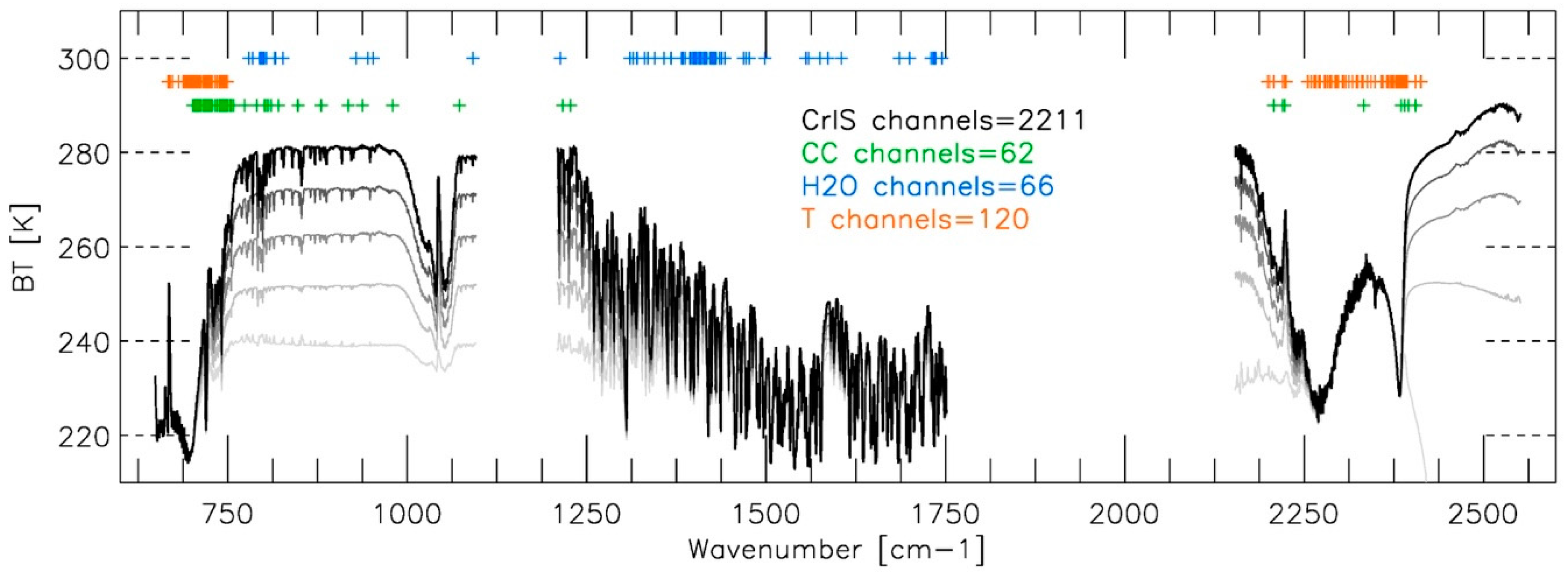
2.1. Hyperspectral Infrared Sounders

Modern era hyperspectral infrared sounders are preceded by the High-Resolution Infrared Radiometer (HIRS), which measures TOA radiance in broad spectral bands with a record that dates back to 1979. It makes an important contribution with its long-term record of retrieved cloud properties [37], but it took the launch of hyperspectral infrared sounders to enable the observation of multiple coincident variables characterizing the atmosphere’s thermodynamic structure and its chemical composition. Hyperspectral measurements with narrow spectral channels characterize atmospheric variables in narrow pressure layers to achieve a vertical resolution of 1 to 5 km depending on height. The sounders on EOS/Aqua, MetOp, SNPP and NOAA-20 satellites (Table 1) have the accuracy and precision to make direct and diagnostic measures of atmospheric change [38]. In sun-synchronous orbits, these observing systems achieve daily global coverage. EOS/Aqua was launched in 2002 with a local overpass time of 13:30. SNPP was launched in 2011 in a similar afternoon orbit with NOAA-20 following in 2017. These instruments have had a large impact on the quality of numerical weather prediction models through the assimilation of channel subsets from cloud-free scenes [14,39,40,41,42]. Moreover, the operational and scientific value of retrieved sounding products is reflected in the literature with studies on a wide range of subjects; from weather and climate feedback studies to regional radiative processes and the forecasting of extreme weather events [17,20,22,43,44,45]. SNPP and EOS/Aqua now have more than seven years of overlap. Demonstrating data continuity between these two platforms is important for extending the record of hyperspectral infrared into future decades when subsequent launches of the CrIS instrument (Table 1) will occur.
Combining multi-instrument products in a long-term record for climate applications, however, is not trivial, as shown for temperature retrievals from CrIS, IASI and AIRS using a statistical regression scheme [10]. This study concludes that despite similar observing capabilities and regression coefficients derived independently for each instrument to promote stability [46,47], a record of temperature retrievals from AIRS, IASI and CrIS do not form a homogenized (continuous) record but instead propagate Level 1 uncertainty that can only be explained by evaluating instrumentation differences. AIRS [48] is a grating spectrometer and integrates its instantaneous Field Of View (FOV) in a spatial point spread function with complicated shape (an oval “tophat” [49]) that overlaps by ~25% along the scanline. CrIS [50] is a Michelson Interferometer and has FOVs that are circular and independent of each other but that rotate along the scanline. Spectrally, CrIS measures each scene with three detectors—longwave, mid-wave and shortwave infrared—whereas AIRS has many detectors that observe radiation in much narrower spectral bands. Each detector has a spatial footprint that varies slightly from all others so in complex cloudy scenes, an AIRS measurement made up of many detector footprints differs from a CrIS measurement of the exact same scene with only three detector footprints. AIRS and CrIS instrument differences can therefore be pronounced in complex cloudy scenes [10]. Other differences involve instrument noise as well as spectral line shapes and resolution.
CLIMCAPS is primarily designed to generate a long-term record of multiple atmospheric ECVs from the AIRS [48] and CrIS [50] but once demonstrated can readily be extended to include IASI (Table 1) for applications that require a higher frequency of observations about the diurnal cycle.

2.2. CLIMCAPS Infrared Inversion System

2.2.1. Bayesian Optimal-Estimation

The inversion of hyperspectral infrared radiance measurements (Level 1) into discrete atmospheric variables (Level 2) is an under-constrained, ill-posed, non-linear problem. We discuss here how inversion can be linearized and regularized (not accounting for iteration) within a Bayesian O-E framework [8] in broad, simplified terms by using the equations as outlined in the seminal text by Rodgers [1]:
x ^ = x a + G ( y y b )
where x ^ and x a are the retrieved and a priori variables, respectively. G (Equation (2)) is the gain matrix that transforms information from radiance space (y) into atmospheric state space (x). The gain matrix is defined as:
G = ( K T S m 1 K + S a 1 ) 1 K S m 1
where K is the Jacobian that describes the sensitivity of forward model calculated radiances ( y b ) to the target variable. Radiative transfer (or forward) models require as input a set of variables that describes the full atmospheric state (background variables, x b , together with target variable, x a ) as close to the true state as possible so that TOA radiances can be calculated with accuracy. S m is the measurement covariance matrix that is made up of a few components including random instrument noise, channel correlation and an estimate of the forward model uncertainty. Each retrieval system defines this matrix differently, depending on their assumptions. Our definition of S m for CLIMCAPS is described below (Figure 1; Section 2.2.4). S a is the a priori covariance matrix that characterizes the uncertainty in the existing knowledge about a target variable. In generic terms, a Bayesian inversion updates the prior estimate of a target variable, xa, with information about the true state of that variable from the TOA radiance measurements, y. The contribution that xa and y respectively make to the final solution are weighted by S a and S m .
One of the most commonly used quality metrics in analysis and assimilation of satellite sounding retrievals is the averaging kernel, A = G K = x ^ x , that describes the sensitivity of the retrieved variable to the true state of that variable. It ranges between 0 and 1 (Figures 4 and 6) and is interpreted as the degree to which the true state is represented in the retrieved solution, i.e., how much information the measurements contributed. If A = 1 , then the measurements completely replace the a priori estimate in the solution. If A = 0 , then the solution is the a priori estimate. Neither of these two extreme cases ever hold true, because the information content of a measurement is never negligible (i.e., where A = 0 and S m ), nor is it ever free of error and uncertainty (i.e., where A = 1 and S m = 0 ).
The error covariance matrix of the inverse solution (Equation (3)), S ^ , for each retrieved variable within a datum is broadly made up of three sources, namely, (i) uncertainty in the “null space”, or that part of the solution without any contribution from the measurement (first term on right-hand side of Equation (3)), (ii) uncertainty about the measurement contribution to the solution (second term), and (iii) uncertainty due to interference from background state variables not directly retrieved (third term).
S ^ = ( A I ) S a ( A I ) T + G S m G T + G K b S b ( G K b ) T
Most retrieval systems only account for the first two components of S ^ by assuming S b to be negligible for the sake of algorithmic simplicity and computational efficiency. While the interference from background variables can be reduced through channel selection, for example, it can never be rendered negligible under all atmospheric conditions. The TOA radiance spectrum is a highly correlated signal of multiple atmospheric state and Earth surface variables. If S b is set to zero then the interference from background state variables are treated as information about the target variable. This spectral correlation between target and background variables in Level 1 radiances will affect the quality of Level 2 products in ways that cannot be quantified a posteriori because it was not propagated explicitly as a source of uncertainty but instead as source of geophysical information about the target variable. This poses a serious risk to data analysis and application, especially once Level 2 retrievals are aggregated into long-term Level 3 and Level 4 CDRs that can amplify systematic effects and lead to misinterpretation and wrong conclusions about trends and cross-correlations in the data. We, therefore, make the case that it is critically important to quantify and propagate all three terms in S ^ (Equation (3)) as rigorously as possible, especially as far as the retrieval of ECVs go. The clear and transparent reporting of all sources of error and uncertainty is vital for promoting understanding and fostering trust in satellite sounding products.

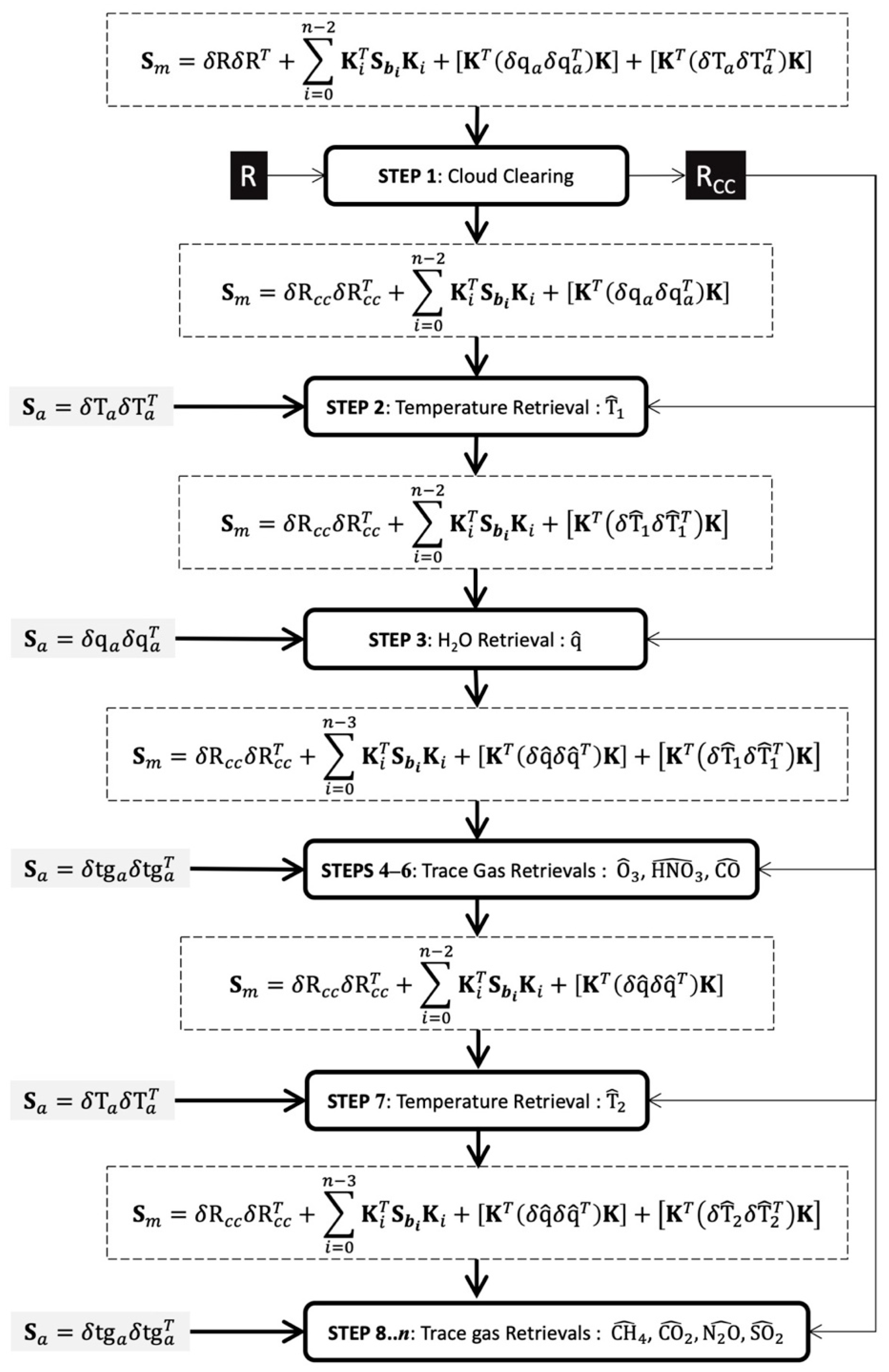
2.2.2. Scene-Dependent Uncertainty Propagation

With scene-dependent uncertainty, we mean the doubt that exists about the full atmospheric state at a specific datum (9 CrIS/AIRS FOVs; ~50 km at nadir; Table 1). It is a source of uncertainty in satellite sounding retrievals because spectral channels are sensitive to multiple atmospheric variables. The target retrieval may be tropospheric water vapor (H2O), but spectral channels sensitive to H2O may simultaneously be sensitive to temperature (CO2 absorption lines) and clouds. A set of channels selected for a target variable may have high information content for a single variable but weak interference from many other state variables. In CLIMCAPS, we implemented a sequential retrieval approach with which to parameterize, quantify and propagate scene-dependent uncertainty so that the retrieved ECVs may be fully characterized and understood. Scene-dependent uncertainty has high variability over time and space and by accounting for it in a transparent and rigorous manner we may correctly interpret variability in CLIMCAPS ECVs from scene-to-scene, day-to-day and year-to-year. Climate science and applications depend on data products where all sources of uncertainty; however small, are propagated rigorously [35,36,51].
In this paper, we describe the CLIMCAPS sequential retrieval approach for temperature and atmospheric gases, water vapor specifically. A description of Earth surface variables—emissivity, reflectivity and skin temperature—is beyond scope. This, along with all relevant technical details, will be covered in full within the CLIMCAPS Algorithm Theoretical Basis Document (ATBD) that is in preparation by the same authors. Broadly speaking, the steps in a CLIMCAPS sequential retrieval are in order as follows: cloud cleared radiances, temperature (T), H2O, O3, CO, HNO3, and then again T, followed by CH4, CO2, SO2 and N2O (Figure 1).
Cloud cleared radiances are retrieved first because they cause the largest source of scene-dependent uncertainty in satellite sounding observations. Spectrally accounting for clouds and quantifying their uncertainty within each datum is key to accurately inverting a TOA radiance spectrum. A scene can be complex (e.g., pyrocumulus clouds over a mega-fire, multi-layer broken cloud fields, severe storm outbreak) or relatively simple (e.g., uniform cirrostratus or altocumulus decks). Once the cloud amount and cloud top pressure are retrieved and removed from the radiance measurement (known as “cloud clearing”, Section 2.2.4), a profile of T is retrieved because a good estimate of scene-dependent temperature is required in the retrieval of all minor gases, including H2O. Following clouds and temperature are H2O, O3, CO, HNO3, in that order (Steps 3–6, Figure 1). Once the column density of these gases is known for the retrieval datum, T is retrieved a second time but with channels sensitive to H2O included because they contain tropospheric T information and help resolve vertical structure in narrower pressure layers. Please note that the second T retrieval uses the same a priori estimate and error covariance matrix (Section 2.2.3) as the first T retrieval, i.e., x a and S a are identical in Steps 2 and 7 (Figure 1). Only the scene-dependent uncertainty and channel set are different.
A sequential retrieval approach has several key benefits. Firstly, it is very fast, because inversion is done one ECV at a time, using only a small subset of channels sensitive to the target ECV, e.g., out of a total of 2211 CrIS channels, CLIMCAPS uses 120 for temperature and 66 for water vapor (Figure 2). These channels are selected for their information content relative to the target EVC as well as their spectral purity, or weak sensitivity to other variables. Secondly, a sequential retrieval is stable and robust because it solves for the most linear components first—retrieving variables with varying degrees of non-linearity simultaneously can cause instability in the solution and mask the real source of uncertainty. Lastly, a sequential approach allows CLIMCAPS to fully characterize and propagate scene-dependent uncertainty from one retrieval step to the next on a per datum basis, because the background error covariance matrix (Sb) can be updated with the retrieval error covariance matrix from the previous step.
The first step is to retrieve the cloud cleared radiances (Step 1, Figure 1). As input, the measurement error covariance matrix, S m , is defined as the sum of the radiance error covariance matrix ( δ R δ R T , Section 2.2.4, Equation (6)) and uncertainty in the background atmospheric state, defined as S b = δ x b δ x b T , where δ x b δ x b T is the a priori error covariance matrices for T, H2O, O3, CO, CO2, N2O, CH4, SO2, and HNO3. The retrieval of all subsequent variables is done with the cloud cleared radiances, which now has its radiance error covariance matrix updated with scene-dependent uncertainty about the state of clouds in the datum ( δ R c c δ R c c T , Section 2.2.4, Equation (7)). Step 2 (Figure 1) is the first T retrieval with measurement error covariance matrix now defined as the sum of δ R c c δ R c c T , and uncertainty in the background atmospheric state as the sum of a priori error covariance matrices for H2O, O3, CO, CO2, N2O, CH4, SO2, and HNO3. Water vapor is retrieved next (Step 3, Figure 1), and this time the background error term is updated with the retrieved temperature error covariance matrix such that S b = δ x b δ x b T + δ   T ^ δ   T ^ T . The same holds for steps 4 through n, where n is the number of retrieved ECVs. Each retrieval step is done retaining the scene-dependent uncertainty from all previous steps and using a different subset of spectral channels depending on the target ECV.
CLIMCAPS retrieved ECVs are characterized with error covariance matrices, averaging kernels, cloud clearing uncertainty, and numerous other diagnostic metrics to enable full uncertainty propagation from Level 2 into subsequent Level 3 and Level 4 climate data records.

2.2.3. Prior Estimate of Atmospheric State

Profiles of temperature and moisture can be derived from TOA infrared radiances using a set of regression coefficients that correlates a measured spectrum with a statistically probable atmospheric state. Both the AST and NUCAPS algorithms use regression retrievals as first guess in their O-E inversion. The AST version 6 algorithm adopted a stratified neural network regression [52,53,54,55,56] while NUCAPS maintains a globally trained linear regression [57]. In general, regression retrieval algorithms can achieve reasonable accuracy as has been demonstrated for NUCAPS, AST and elsewhere in the direct-broadcast Community Satellite Processing System’s Dual-Regression (CSPP) [16,46,47,57,58,59]. A statistical regression retrieval, however, is inappropriate as an a priori constraint for CLIMCAPS retrievals for several important reasons (outlined in Table 2). A regression retrieval is highly scene-dependent, but its uncertainty can only be calculated statistically for a large ensemble afterwards and thus cannot be known at the time of retrieval. Moreover, it depends on the very same radiance measurements from which the variables are retrieved in the O-E inversion step. This means that it not only enhances instrument effects but also propagates and even amplifies the scene-dependent error and correlation among state variables. CLIMCAPS requires an a priori estimate and associated error covariance matrix that is largely independent of the spectral measurements and retrieval datum (space and time) so that all scene-dependent uncertainty can be attributed to known sources and carefully propagated. It is important that all sources of uncertainty can be fully characterized in the retrieved ECVs to help make sense of differences when compared to other ECVs and CDRs. We selected MERRA2 reanalysis product [60,61] as CLIMCAPS a priori estimate for temperature and water vapor and below give a detailed breakdown of the reasons why (Table 1).
We calculate the a priori error covariance matrix (Figure 3) for temperature and water vapor from an ensemble (233,135 profiles) of differences between the European Center for Medium-Range Weather Forecasts (ECMWF) [62,63] and MERRA2 from four global focus days in 2015—1 January, 1 April, 1 July and 1 October. ECMWF serves as an estimate of the true atmospheric state and a benchmark for the best estimate of the atmospheric state at the space-time resolution of AIRS and CrIS (~50 km at nadir, twice a day). Before differencing, the ECMWF and MERRA2 profiles are spatially and temporally interpolated with the AIRS (or CrIS) space-time resolution. They are then vertically interpolated with the 100-level retrieval pressure grid and smoothed using a 3-point running mean to remove random noise effects. All profiles where MERRA2 and ECMWF differences exceed 10 K in temperature or 500% in water vapor are rejected. In the upper stratosphere (< 50 hPa), the typically large differences in model profiles taper off.
The a priori error covariance matrix (Figure 3) for temperature and water vapor remains static from datum to datum because MERRA2 uncertainty does not vary at the same scale of the AIRS and CrIS measurements. With MERRA2 as a priori estimate and its static error covariance matrix in the CLIMCAPS inversion system, we can be sure that all scene-dependent uncertainty and variability in the retrieved ECVs come from the radiance measurements alone.

2.2.4. Cloud Clearing

Clouds cause the highest scene-dependent uncertainty in sounding observations from space-borne infrared instruments [10,25,26,27,47,64,65,66,67]. By clouds, we mean any type of cloud, fog or smoke that prevent a “spectral” view of the Earth surface. There are three main approaches to clouds in retrieval systems today: (i) avoid cloudy scenes, (ii) model the full suite of cloud parameters, or (iii) remove cloud effects from measured spectra. Each of these choices holds significant implications for the quality and nature of retrieved ECVs and derived CDRs.
Clouds can be avoided altogether by limiting sounding retrievals to clear-sky atmospheres. This is the simplest approach because the inversion of clear sky radiances is a well-known problem and can be done with high accuracy. However, avoiding cloudy scenes means that every day a significant portion of the global atmosphere is not observed, thus causing large systematic sampling errors in long-term records because the number of clear-sky CLIMCAPS soundings is typically 5% on any given global day. Modelling clouds, on the other hand, is the most complex approach, since the effects of clouds on infrared radiances are very difficult to deconvolve. Soundings can be retrieved in the presence of clouds but at the risk of introducing large systematic errors due to the fact that the infrared sounding of clouds is highly under-constraint and strongly dependent on inversion constraints. These include robust a priori estimates of cloud amount, height and optical properties as well as forward models that accurately calculate radiative transfer through clouds, which is an exceedingly complex problem with large associated uncertainties.
There are retrieval methods that attempt to directly solve for clouds using single footprint infrared radiances [68,69] but these are experimental at best and do not quantify or propagate cloud uncertainty rigorously enough for ECVs at global scales. The CLIMCAPS inversion system, instead, adopts a “cloud clearing” approach, which was developed in the 1970s [70,71,72] and is still operational today [2,29]. Cloud clearing removes the radiative effect of clouds from the infrared measurements without requiring knowledge of complex cloud parameters such as single scattering albedo, cloud phase or cloud density as a function of height for multiple cloud particle types. Perhaps the most significant advantage is that cloud clearing uncertainty can be accurately quantified for each datum and then propagated into subsequent retrieval steps so that ECV information content may be maximized.
The basic assumption of cloud clearing is that within a retrieval datum, the cloud types are constant and only the cloud fraction varies. With nine AIRS (or CrIS) FOVs within each datum (~50 km at nadir, Table 1) there is a high probability that the cloud fraction in at least one FOV varies from the rest. For all scenes with some contrast in cloud cover, a single cloud cleared radiance spectrum can be retrieved from the nine FOVs using a linear least squares approach. Geophysically, this is reasonable, because TOA infrared spectra respond proportionally to the amount of clouds in the measured footprint (Section 2.2.2; Figure 2). In this sense, the cloud clearing algorithm uses a datum’s “spatial information content” (spatial heterogeneity in cloud sensitive channels) not the “spectral information content” (radiative sensitivity to cloud type, height and optical properties). The spatial information content is high where a datum is partly filled with clouds and the spectral differences among the nine FOVs are high as a result (Figure 2 illustrates how spectra are proportional to percent cloud cover). With nine FOVs sampling a partly cloudy scene, cloud clearing finds a cloud-free radiative pathway past the clouds from TOA to Earth surface. Spatial information content is low when a datum is homogeneous with no variation in cloud amount and thus no variation in cloud sensitive channels from FOV to FOV. This happens in the presence of uniform cloud decks (100% cloudy) or where each FOV is covered by the same amount of clouds (e.g., when all nine FOVs have 40% cloud cover). The dependence on spatial information content makes cloud clearing robust even in very complex cloudy scenes because it requires no information about the amount, height or optical properties of clouds. However, the downside is that the spectral region sensitive to clouds is also sensitive to the lower troposphere and Earth Surface. This means that a datum over coastlines, with part water part land, can be mistaken for a cloudy scene (large differences in CC spectral channels from FOV to FOV; Figure 1), or alternatively, very low clouds (e.g., in boundary layer) can be mistaken as a cool clear-sky scene.
A cloud cleared radiance spectrum ( R C C ) is a least squares linear combination of the nine FOVs within each CLIMCAPS datum (Equations (4) and (5)). It is described in detail elsewhere [2], but will we give a brief overview here for the sake of clarity. A cloud cleared radiance spectrum, R cc , is derived from nine FOVs as follows:
R C C = R ¯ + j = 1 9 η j ( R ¯ R j )
where R ¯ is the average radiance in a datum, R j is one of nine measured FOV radiance spectra, and η j the least squares approximation derived for each datum ( 3 × 3 FOV), as follows:
η j = [ ( R ¯ R j ) T δ R δ R T ( R ¯ R j ) + λ ] 1 ( R ¯ R j ) T δ R δ R T ( R x b R ¯ )
with λ being the regularization factor and x b the background atmospheric state used to calculate a clear-sky TOA spectrum. δ R δ R T is the measurement uncertainty (Equation (6)), and defined as the sum of the average random instrument noise component (NE Δ N) and the forward model uncertainty calculated off-line for an ensemble of cases and held constant through all retrievals.
δ R δ R T = 1 9 ( N E Δ T ) C ( N E Δ T ) + ε
where C is the channel correlation matrix and for AIRS is the identity matrix and CrIS the apodization correlation matrix. S m is therefore a combination of random noise (NE Δ N), channel correlation (C) and systematic effects due to assumptions in the radiative transfer model ( ε ). δ R δ R T is updated for the retrieved cloud cleared radiances as follows:
δ R c c δ R c c T = A ( N E Δ N ) C ( N E Δ T ) + S r ( δ η δ η T ) S r T + ε
with A a scalar that quantifies the amplification in random noise due to cloud clearing (see [2] for a detailed discussion), δ η δ η T the least squares error covariance matrix ( 9 × 9 ) and S r the transformation matrix from FOV to spectral space with N channels:
S r = ( R 1 ¯ R 1 , 9 R 1 ¯ R 1 , 1 R N ¯ R N , 9 R N ¯ R N , 1 )
CLIMCAPS uses R cc and R j to calculate cloud top pressure for up to two layers as well as up to 18 effective radiative cloud fractions to help diagnose product quality and scene complexity in subsequent research studies.

3. Results and Discussion

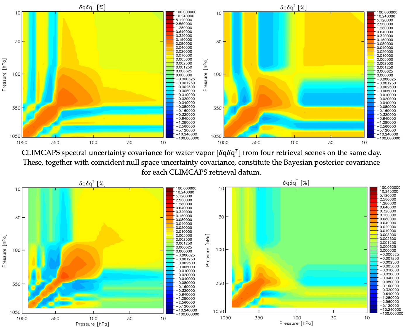
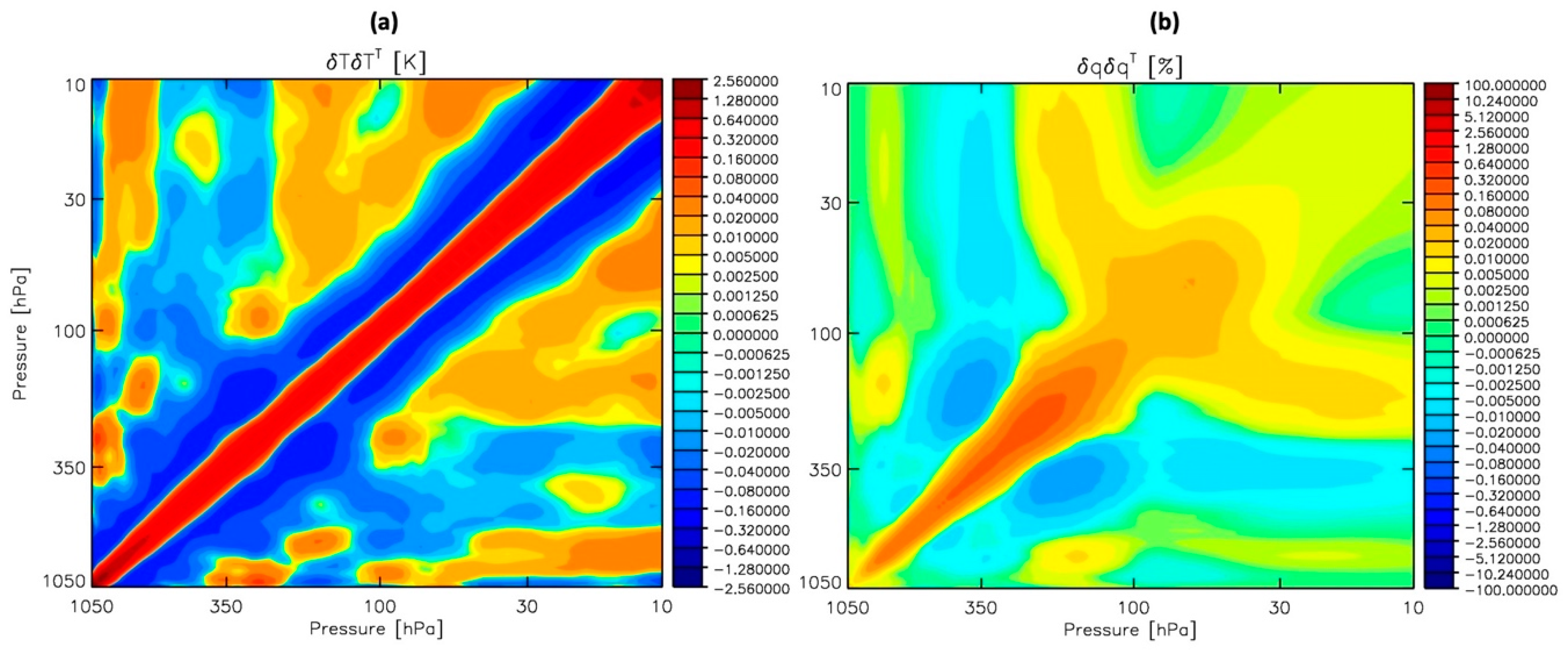
3.1. Datum-Specific Uncertainty Metrics

The sensitivity of TOA infrared radiance to the atmospheric state varies depending on localized conditions, e.g., the higher the load of CO molecules in the upper troposphere (e.g., due to a large fire event), the stronger its spectral signature in the 2150 cm−2 wavenumber region; or, the larger the difference in temperature between Earth surface and boundary layer, the higher the sensitivity to fine-scale thermodynamic structures, and so on. The Bayesian averaging kernel ( A ; Section 2.2.1) has found widespread use in the weather and climate communities as an intuitive metric of uncertainty. CLIMCAPS follows the AST and NUCAPS approach in calculating A [73]. The diagonal vector of A (Figure 4) is the degree to which measurements contribute to the final solution as a function of pressure. A Bayesian retrieval (Section 2.2.1) at specific pressure level, P ( l ) , has total information content equal to unity, with a weighted contribution from the measurements equal to A ( l , l ) and a weighted contribution from the a priori estimate equal to [ 1 A ( l , l ) ] . In this way, A is a metric of the scene-dependent measurement information content within a datum, i.e., the amount of unique information contributed by the measurement given the constraints imposed by the inversion algorithm (e.g., channel selection and choice of a priori). Alternatively, when considering retrieval uncertainty at P ( l ) , then A ( l , l ) quantifies the fraction contributed by S m , and [ 1 A ( l , l ) ] represents the null space and quantifies the fraction contributed by S a .
For a target variable, A is not constant (Figure 4) because it depends on, (i) the accuracy of the a priori estimate, as well as (ii) the information content in the measurements at a given point in time and space. If the a priori estimate approximates the true state, then A 0 irrespective of the information content in the measurement about the target variable, because the true state is already known and no new information can be added from the measurements to improve it. Alternatively, if the a priori estimate is a generalized climatology and do not resemble localized conditions, then A 1 if the measurement information content about a target variable is high, but A 0 if its low, irrespective of the quality of the a priori estimate. A is thus a complex metric and in isolation does not fully characterize the retrieved ECV uncertainty; it should only be interpreted within the context of the retrieval system and assumptions made within. It is for this reason that a one-to-one comparison between A s from different retrieval systems do not yield much insight and should never be mistaken as an indicator of the accuracy of the retrieved variable. The CLIMCAPS A for temperature (Figure 4, top row) is relatively stable across pressure levels and latitudinal zones as indicated by the narrow error bars. For water vapor (Figure 4, bottom row), the A has high variability, both vertically and spatially. A map of the total vertical information content, known as the degrees of freedom and calculated as the sum of the A diagonal, A ( l , l ) , reveal spatial patterns of uncertainty in temperature and water vapor (Figure 5).
As discussed above (Section 2.2.2, Figure 1), the retrieval of temperature is done in two separate steps; the first temperature retrieval contains scene-dependent uncertainty about clouds only while using static uncertainty estimates for all background variables, namely H2O, CO, O3 and HNO3. The second temperature retrieval updates its scene-dependent uncertainty estimates for clouds as well as the background variables. Scene-dependent knowledge of tropospheric H2O enables the inclusion of additional channels—sensitive to both temperature and H2O—so that thermodynamic structure may be retrieved with higher vertical resolution. The reason for this multi-step iteration in temperature can perhaps be best understood with averaging kernels (Figure 6), where we see an increase in tropospheric values of A once scene-dependent knowledge about clouds and trace gases were fully characterized (magenta lines).
CLIMCAPS calculates and outputs an error covariance matrix, S ^ , for each retrieved ECV at every datum. Broadly speaking, S ^ is the sum of three sources of uncertainty (Section 2.2.1; Equation (3)) namely, the null space ( I A ) , instrumentation as well as interference from background state variables. In CLIMCAPS we combine the latter two terms into one term since they are both spectrally based (Section 2.2.2). For temperature, the null space error covariance matrix is high (Figure 7a) and weakly correlated, whereas the magnitude of the spectral error covariance matrix is lower (Figure 7b) with stronger correlation, especially in the stratosphere. For tropospheric H2O (Figure 8c,d), the contribution from the two sources of uncertainty are similar in magnitude but correlation is introduced by uncertainty propagated from the measurements (broader orange feature in Figure 7d). All these sources of uncertainty and error contribute to the magnitude and structure of the averaging kernel of a retrieved ECV at a specific datum in time and space.
The averaging kernels for three different CLIMCAPS scenes highlight the scene-dependence of information content (Figure 6). For the same three scenes, we can evaluate the null space and spectral error covariance matrices, respectively, to help understand the retrieval and its A better (Figure 8).

3.2. Retrieved Essential Climate Variables—Temperature and Water Vapor

One of the dominant sources of uncertainty in satellite sounding retrievals is tied to local weather conditions, and therefore are highly variable from datum to datum and day to day. How, then, can we assemble CDRs from satellite soundings to characterize long-term and large-scale patterns and processes? How can we use data whose quality depends on weather patterns in climate research? The answer is simple but not trivial: with rigorous uncertainty characterization, propagation and reporting. Knowledge about uncertainty in ECVs is as important as the retrieved quantity itself [35,36,51].
We designed CLIMCAPS to retrieve ECVs that can be assembled into CDRs for the study of feedback cycles and other climate processes, by adopting two key design elements that distinguishes it from other operational retrieval systems, such as NUCAPS and AST. These are, (i) an a priori estimate that is largely independent of the same sources of scene-dependent uncertainty as the measurements, and (ii) the sequential retrieval of multiple ECVs from a single measurement with full uncertainty propagation to account for all sources of scene-dependent effects.
We can demonstrate the value of CLIMCAPS with a statistical analysis of retrieved temperature and water vapor for the six global days from Aqua/AIRS and SNPP/CrIS spanning all four seasons: 1 July 2013, 1 January 2015, 1 April 2015, 1 July 2015, 1 October 2015 and 14 January 2016. In order to highlight the differences between CLIMCAPS and inversion systems that employ statistical a priori estimates for temperature and water vapor without formal error propagation, we compared CLIMCAPS against NUCAPS, We also compared NUCAPS and AST v.6, and can confirm that the retrievals from these systems yield similar results for the same six global days (not shown).
With respect to ECMWF, NUCAPS temperature T(p) error (bias) oscillates between −1K and 1K for day and night, while CLIMCAPS T(p) error (bias) remains within an 0.5 K irrespective of time of day (Figure 9). CLIMCAPS uncertainty (precision or standard deviation) for T(p) is less than half that of NUCAPS, which routinely exceed 1.5K in the boundary layer. With a statistical regression a priori estimate, NUCAPS scene-dependent variation in information content is amplified because the measured spectrum of a single footprint is used twice, first in deriving the statistical a priori that uses all spectral channels and then in the O-E retrieval of the final state (Section 2.2.1). This means that variation in retrieval quality from footprint to footprint is high because measurements with low information content will result in high retrieval uncertainty and vice versa. This is not the case for CLIMCAPS that has MERRA2 reanalysis as a priori. In CLIMCAPS only a small fraction of the measured spectrum is used twice. MERRA2 assimilates a small subset of AIRS and CrIS channels and it does so for clear-sky scenes only. Moreover, AIRS and CrIS are only two of many different instruments that MERRA2 assimilates; the contribution from any one instrument to a MERRA2 modelled state at any point in time is thus very low. NUCAPS temperature and moisture retrievals has high scene-dependent variability as quantified by the standard deviation with respect to ECMWF for different latitudinal zones (polar versus mid-latitude) and surface types (land versus ocean). On the other hand, CLIMCAPS statistics for the same scenes are consistently lower with minimal variability along the vertical axis (Figure 10).
For the same set of focus days and ECMWF as estimate of the true state, we can illustrate how CLIMCAPS, unlike NUCAPS, achieves consistency in retrieved ECVs between two different instruments—Aqua/AIRS and SNPP/CrIS. The NCAPS global temperature, T(p), error profiles of AIRS and CrlS (Figure 11a) have strong variations with pressure that ranges between −1K and 1K. The vertical distribution of these variations from AIRS are different from those of CrlS. The NUCAPS global moisture, Q(p), error profiles have similar mismatches in vertical error (bias) between AIRS and CrIS, albeit with lower variation than T(p). The CLIMCAPS global T(p) and Q(p) error profiles (Figure 11b) are similar for AIRS and CrIS. We see this retrieval error consistency for CLIMCAPS across instruments also within latitudinal zones (Figure 12).
In summary, CLIMCAPS minimizes the propagation of scene-dependent spectral uncertainty by having an a priori estimate for temperature and water vapor that is largely independent of the spectral measurements. NUCAPS, on the other hand, uses the full set of AIRS and CrIS spectral channels in deriving its a priori estimate for temperature and water vapor, thus amplifying scene-dependent errors and uncertainty. CLIMCAPS also quantifies and propagates uncertainty due spectral interference from background state variables, which means that during inversion this spectral component can be correctly assigned as uncertainty about the retrieved variable. If the spectral interference from background state variables is not explicitly quantified in the Bayesian equation, then it is treated as information about the retrieved variable during inversion. This not only introduces instabilities in the retrieval system, but perhaps most importantly, affects product uncertainty estimates in a way that confounds understanding and can lead to misinterpretations in climate applications and scientific research.

4. Conclusions

The Community Long-term Infrared Microwave Combined Atmospheric Product System (CLIMCAPS) retrieves multiple Essential Climate Variables (ECV) from measurements made by modern-era microwave and hyperspectral infrared sounding instruments on low-Earth orbiting satellites. These are profiles of temperature and water vapor, column amounts of greenhouse gases (CO2, CH4), ozone (O3) and precursor gases (CO, SO2) as well as cloud properties. The hyperspectral Atmospheric InfraRed Sounder (AIRS) was the first instrument of its kind and launched in 2002 on the Aqua satellite. Its successor, the Cross-track Infrared Sounder (CrIS), has been in similar orbit since 2011. Plans are in place to continue this atmospheric sounding capability well into the 2040s. CLIMCAPS retrieves ECVs from both AIRS and CrIS so that a multi-decadal Climate Data Record (CDR) may be assembled.
The unique contribution we make with this paper is to discuss how scene-dependent uncertainty can be quantified and systematically propagated through a satellite sounding retrieval system to decompose a highly correlated spectral signature (Level 1) into multiple ECVs (Level 2) with minimal correlation. We demonstrate how the correct treatment of scene-dependent spectral effects result in retrieval products that have global consistency across seasons and instruments.
Future work will focus on validating CLIMCAPS Level 2 scene-dependent uncertainty estimates by using measurements from numerous field campaigns. Once validated, we will develop a methodology with which to rigorously propagate Level 2 uncertainty into Level 3 and Level 4 CDRs to support the study of complex feedback cycles and to characterize the climate system with multiple thermodynamically consistent ECVs.

Author Contributions

Conceptualization, both authors.; methodology, C.D.B.; software, both authors; formal analysis, N.S.; investigation, both authors; writing—original draft preparation, N.S.; writing—review and editing, N.S.; visualization, both authors; funding acquisition, C.D.B. (Principal Investigator) and N.S. (Co-Investigator).

Funding

This research was funded by NASA, grant award number 80NSSC18K0975.

Acknowledgments

We would like to thank the three anonymous reviewers who contributed meaningfully and helped to substantially improve the quality of this paper.

Conflicts of Interest

The authors declare no conflict of interest. The funding agency had had no role in the design of the CLIMCAPS algorithm approach or products; in the collection, analysis or interpretation of data; in the writing of this manuscript or the decision to publish these results.

References

  1. Bowman, K.W.; Rodgers, C.D.; Kulawik, S.S.; Worden, J.; Sarkissian, E.; Osterman, G.; Steck, T.; Ming, L.; Eldering, A.; Shephard, M.; et al. Tropospheric emission spectrometer: Retrieval method and error analysis. IEEE Trans. Geosci. Remote Sens. 2006, 44, 1297–1307. [Google Scholar] [CrossRef]
  2. Susskind, J.; Barnet, C.D.; Blaisdell, J.M. Retrieval of atmospheric and surface parameters from AIRS/AMSU/HSB data in the presence of clouds. IEEE Trans. Geosci. Remote Sens. 2003, 41, 390–409. [Google Scholar] [CrossRef]
  3. Deeter, M.N. Operational carbon monoxide retrieval algorithm and selected results for the MOPITT instrument. J. Geophys. Res. 2003, 108. [Google Scholar] [CrossRef]
  4. Deeter, M.N.; Edwards, D.P.; Gille, J.C.; Emmons, L.K.; Francis, G.; Ho, S.-P.; Mao, D.; Masters, D.; Worden, H.; Drummond, J.R.; et al. The MOPITT version 4 CO product: Algorithm enhancements, validation, and long-term stability. J. Geophys. Res. 2010, 115. [Google Scholar] [CrossRef] [Green Version]
  5. Rodgers, C.D. Retrieval of atmospheric temperature and composition from remote measurements of thermal radiation. Rev. Geophys. 1976, 14, 609–624. [Google Scholar] [CrossRef]
  6. Rodgers, C.D. Characterization and error analysis of profiles retrieved from remote sounding measurements. J. Geophys. Res. 1990, 95, 5587–5595. [Google Scholar] [CrossRef]
  7. Rodgers, C.D. Information content and optimisation of high spectral resolution remote measurements. Adv. Space Res. 1998, 21, 361–367. [Google Scholar] [CrossRef]
  8. Rodgers, C.D. Inverse Methods for Atmospheric Sounding: Theory and Practice; World Scientific: Singapore; Hackensack, NJ, USA, 2000; ISBN 978-981-02-2740-1. [Google Scholar]
  9. GCOS. Systematic Observation Requirements for Satellite-BASED products for Climate; WMO GCOS: Geneva, Switzerland, 2011; p. 127. [Google Scholar]
  10. Smith, N.; Smith, W.L.; Weisz, E.; Revercomb, H.E. AIRS, IASI and CrIS retrieval records at climate scales: An investigation into the propagation systematic uncertainty. J. Appl. Meteorol. Climatol. 2015, 54, 1465–1481. [Google Scholar] [CrossRef]
  11. Gaudel, A.; Cooper, O.R.; Ancellet, G.; Barret, B.; Boynard, A.; Burrows, J.P.; Clerbaux, C.; Coheur, P.-F.; Cuesta, J.; Cuevas, E.; et al. Tropospheric Ozone Assessment Report: Present-day distribution and trends of tropospheric ozone relevant to climate and global atmospheric chemistry model evaluation. Elem. Sci. Anth. 2018, 6, 39. [Google Scholar] [CrossRef]
  12. Shephard, M.W.; Cady-Pereira, K.E. Cross-track Infrared Sounder (CrIS) satellite observations of tropospheric ammonia. Atmos. Meas. Tech. 2015, 8, 1323–1336. [Google Scholar] [CrossRef] [Green Version]
  13. Gambacorta, A.; Barnet, C.D. Methodology and Information Content of the NOAA NESDIS Operational Channel Selection for the Cross-Track Infrared Sounder (CrIS). IEEE Trans. Geosci. Remote Sens. 2013, 51, 3207–3216. [Google Scholar] [CrossRef]
  14. Chahine, M.T.; Pagano, T.S.; Aumann, H.H.; Atlas, R.; Barnet, C.; Blaisdell, J.; Chen, L.; Divakarla, M.; Fetzer, E.J.; Goldberg, M.; et al. AIRS: Improving Weather Forecasting and Providing New Data on Greenhouse Gases. Bull. Am. Meteorol. Soc. 2006, 87, 911–926. [Google Scholar] [CrossRef]
  15. Weisz, E.; Smith, N.; Smith, W.L.; Strabala, K.; Huang, H.L. Assessing Hyperspectral Retrieval Algorithms and Their Products for Use in Direct Broadcast Applications. In Proceedings of the 20th International TOVS Study Conference (ITSC-20) Proceedings, Lake Geneva, WI, USA, 28 October–3 November 2015. [Google Scholar]
  16. Weisz, E.; Smith, N.; Smith, W.L. The use of hyperspectra sounding information to monitor atmospheric tendencies leading to severe local storms. Earth Space Sci. 2015, 2, 369–377. [Google Scholar] [CrossRef]
  17. Berndt, E.; Folmer, M. Utility of CrIS/ATMS profiles to diagnose extratropical transition. Results Phys. 2018, 8, 184–185. [Google Scholar] [CrossRef]
  18. Berndt, E.B.; Zavodsky, B.T.; Folmer, M.J. Development and Application of Atmospheric Infrared Sounder Ozone Retrieval Products for Operational Meteorology. IEEE Trans. Geosci. Remote Sens. 2016, 54, 958–967. [Google Scholar] [CrossRef]
  19. Smith, W.L. Atmospheric soundings from satellites—False expectation or the key to improved weather prediction? Q. J. R. Meteorol. Soc. 1991, 117, 267–297. [Google Scholar]
  20. Iturbide-Sanchez, F.; da Silva, S.R.S.; Liu, Q.; Pryor, K.L.; Pettey, M.E.; Nalli, N.R. Toward the Operational Weather Forecasting Application of Atmospheric Stability Products Derived from NUCAPS CrIS/ATMS Soundings. IEEE Trans. Geosci. Remote Sens. 2018, 56, 4522–4545. [Google Scholar] [CrossRef]
  21. Smith, N.; White, K.D.; Berndt, E.B.; Zavodsky, B.T.; Wheeler, A.; Bowlan, M.A.; Barnet, C.D. NUCAPS in AWIPS–Rethinking information compression and distribution for fast decision making. In Proceedings of the 98th America Meteorological Society Annual Meeting, Austin, TX, USA, 7–11 January 2018. [Google Scholar]
  22. Smith, N.; Berndt, E.B.; Barnet, C.D.; Goldberg, M.D. Why operational meteorologists need more satellite soundings. In Proceedings of the 99th America Meteorological Society Annual Meeting, Phoenix, AZ, USA, 6–10 January 2019. [Google Scholar]
  23. Ackerman, S.A.; Platnick, S.; Bhartia, P.K.; Duncan, B.; L’Ecuyer, T.; Heidinger, A.; Skofronick-Jackson, G.; Loeb, N.; Schmit, T.; Smith, N. Satellites See the World’s Atmosphere. Meteorol. Monogr. 2018, 59, 4.1–4.53. [Google Scholar] [CrossRef]
  24. Rodgers, C.D. Remote sensing of the atmospheric temperature profile in the presence of cloud. Q. J. R. Meteorol. Soc. 1970, 96, 654–666. [Google Scholar] [CrossRef]
  25. Eyre, J.R. The information content of data from satellite sounding systems: A simulation study. Q. J. R. Meteorol. Soc. 1990, 116, 401–434. [Google Scholar] [CrossRef]
  26. Eyre, J.R. Inversion of cloudy satellite sounding radiances by nonlinear optimal estimation. I: Theory and simulation for TOVS. Q. J. R. Meteorol. Soc. 1989, 115, 1001–1026. [Google Scholar] [CrossRef]
  27. Eyre, J.R. Inversion of cloudy satellite sounding radiances by nonlinear optimal estimation. II: Application to TOVS data. Q. J. R. Meteorol. Soc. 1989, 115, 1027–1037. [Google Scholar] [CrossRef]
  28. Susskind, J.; Blaisdell, J.M.; Iredell, L. Improved methodology for surface and atmospheric soundings, error estimates, and quality control procedures: The atmospheric infrared sounder science team version-6 retrieval algorithm. J. Appl. Remote Sens. 2014, 8, 084994. [Google Scholar] [CrossRef]
  29. Susskind, J.; Blaisdell, J.M.; Iredell, L.; Keita, F. Improved Temperature Sounding and Quality Control Methodology Using AIRS/AMSU Data: The AIRS Science Team Version 5 Retrieval Algorithm. IEEE Trans. Geosci. Remote Sens. 2011, 49, 883–907. [Google Scholar] [CrossRef]
  30. Goldberg, M.D.; Kilcoyne, H.; Cikanek, H.; Mehta, A. Joint Polar Satellite System: The United States next generation civilian polar-orbiting environmental satellite system: USA NEXT GENERATION SATELLITE SYSTEM. J. Geophys. Res. Atmos. 2013, 118, 13463–13475. [Google Scholar] [CrossRef]
  31. Sun, B.; Reale, A.; Tilley, F.H.; Pettey, M.E.; Nalli, N.R.; Barnet, C.D. Assessment of NUCAPS S-NPP CrIS/ATMS Sounding Products Using Reference and Conventional Radiosonde Observations. IEEE J. Sel. Top. Appl. Earth Obs. Remote Sens. 2017, 10, 2499–2509. [Google Scholar] [CrossRef]
  32. Nalli, N.R.; Gambacorta, A.; Liu, Q.; Barnet, C.D.; Tan, C.; Iturbide-Sanchez, F.; Reale, T.; Sun, B.; Wilson, M.; Borg, L.; et al. Validation of Atmospheric Profile Retrievals from the SNPP NOAA-Unique Combined Atmospheric Processing System. Part 1: Temperature and Moisture. IEEE Trans. Geosci. Remote Sens. 2018, 56, 180–190. [Google Scholar] [CrossRef]
  33. Nalli, N.R.; Gambacorta, A.; Liu, Q.; Tan, C.; Iturbide-Sanchez, F.; Barnet, C.D.; Joseph, E.; Morris, V.R.; Oyola, M.; Smith, J.W. Validation of Atmospheric Profile Retrievals from the SNPP NOAA-Unique Combined Atmospheric Processing System. Part 2: Ozone. IEEE Trans. Geosci. Remote Sens. 2018, 56, 598–607. [Google Scholar] [CrossRef]
  34. Trenberth, K.E.; Anthes, R.A.; Belward, A.; Brown, O.B.; Habermann, T.; Karl, T.R.; Running, S.; Ryan, B.; Tanner, M.; Wielicki, B. Challenges of a Sustained Climate Observing System. In Climate Science for Serving Society; Asrar, G.R., Hurrell, J.W., Eds.; Springer: Dordrecht, The Netherlands, 2013; pp. 13–50. ISBN 978-94-007-6691-4. [Google Scholar] [Green Version]
  35. Merchant, C.J.; Paul, F.; Popp, T.; Ablain, M.; Bontemps, S.; Defourny, P.; Hollmann, R.; Lavergne, T.; Laeng, A.; de Leeuw, G.; et al. Uncertainty information in climate data records from Earth observation. Earth Syst. Sci. Data 2017, 9, 511–527. [Google Scholar] [CrossRef] [Green Version]
  36. Mittaz, J.; Merchant, C.J.; Woolliams, E.R. Applying principles of metrology to historical Earth observations from satellites. Metrologia 2019. [Google Scholar] [CrossRef]
  37. Wylie, D.; Jackson, D.L.; Menzel, W.P.; Bates, J.J. Trends in Global Cloud Cover in Two Decades of HIRS Observations. J. Clim. 2005, 18, 3021–3031. [Google Scholar] [CrossRef]
  38. Pierrehumbert, R.T.; Hafemeister, D.; Kammen, D.; Levi, B.G.; Schwartz, P. Infrared Radiation and Planetary Temperature. AIP Conf. Proc. 2011, 1401, 232–244. [Google Scholar]
  39. Smith, W.L.; Revercomb, H.E.; Bingham, G.; Larar, A.; Huang, H.L.; Zhou, D.K.; Li, J.; Liu, X.; Kireev, S.V. Technical note: Evolution, current capabilities, and future advance in satellite nadir viewing ultra-spectral IR sounding of the lower atmopshere. Atmos. Chem. Phys. 2009, 9, 5563–5574. [Google Scholar] [CrossRef]
  40. Le Marshall, J.; Jung, J.; Derber, J.; Chahine, M.; Treadon, R.; Lord, S.J.; Goldberg, M.; Wolf, W.; Liu, H.C.; Joiner, J.; et al. Improving Global Analysis and Forecasting with AIRS. Bull. Am. Meteorol. Soc. 2006, 87, 891–895. [Google Scholar] [CrossRef] [Green Version]
  41. Jones, T.A.; Stensrud, D.J. Assimilating AIRS Temperature and Mixing Ratio Profiles Using an Ensemble Kalman Filter Approach for Convective-Scale Forecasts. Weather Forecast. 2012, 27, 541–564. [Google Scholar] [CrossRef]
  42. Collard, A.D.; Healy, S.B. The combined impact of future space-based atmospheric sounding instruments on numerical weather-prediction analysis fields: A simulation study. Q. J. R. Meteorol. Soc. 2003, 129, 2741–2760. [Google Scholar] [CrossRef]
  43. Gettelman, A.; Fu, Q. Observed and Simulated Upper-Tropospheric Water Vapor Feedback. J. Clim. 2008, 21, 3282–3289. [Google Scholar] [CrossRef] [Green Version]
  44. Fasullo, J.T.; Trenberth, K.E. A Less Cloudy Future: The Role of Subtropical Subsidence in Climate Sensitivity. Science 2012, 338, 792–794. [Google Scholar] [CrossRef] [PubMed]
  45. Dessler, A.E.; Zhang, Z.; Yang, P. Water-vapor climate feedback inferred from climate fluctuations, 2003–2008. Geophys. Res. Lett. 2008, 35. [Google Scholar] [CrossRef]
  46. Smith, W.L.; Weisz, E.; Kireev, S.V.; Zhou, D.K.; Li, Z.; Borbas, E.E. Dual-regression retrieval algorithm for real-time processing of satellite ultraspectral radiances. J. Appl. Meteorol. Climatol. 2012, 51, 1455–1476. [Google Scholar] [CrossRef]
  47. Weisz, E.; Smith, W.L.; Smith, N. Advances in simultaneous atmospheric profile and cloud parameter regression based retrieval from high-spectral resolution radiance measurements. J. Geophys. Res. Atmos. 2013, 118, 6433–6443. [Google Scholar] [CrossRef]
  48. Aumann, H.H.; Chahine, M.T.; Gautier, C.; Goldberg, M.D.; Kalnay, E.; McMillin, L.M.; Revercomb, H.; Rosenkranz, P.W.; Smith, W.L.; Staelin, D.H.; et al. AIRS/AMSU/HSB on the aqua mission: Design, science objectives, data products, and processing systems. IEEE Trans. Geosci. Remote Sens. 2003, 41, 253–264. [Google Scholar] [CrossRef]
  49. Pagano, T.S.; Aumann, H.H.; Manning, E.M.; Elliott, D.A.; Broberg, S.E. Improving AIRS Radiance Spectra in High Contrast Scenes Using MODIS. In Proceedings of the SPIE 9607, Earth Observing Systems XX, San Diego, CA, USA, 8 September 2015; p. 96070K. [Google Scholar]
  50. Glumb, R.J.; Jordan, D.C.; Mantica, P. Development of the Crosstrack Infrared Sounder (CrIS) Sensor Design. In Proceedings of the SPIE 4486, Infrared Spaceborne Remote Sensing IX, San Diego, CA, USA, 8 February 2002; pp. 411–424. [Google Scholar]
  51. Merchant, C.; Holl, G.; Mittaz, J.; Woolliams, E. Radiance Uncertainty Characterisation to Facilitate Climate Data Record Creation. Remote Sens. 2019, 11, 474. [Google Scholar] [CrossRef]
  52. Blackwell, W.J. Neural network Jacobian analysis for high-resolution profiling of the atmosphere. EURASIP J. Adv. Signal Process. 2012, 2012, 71. [Google Scholar] [CrossRef] [Green Version]
  53. Blackwell, W.J. Validation of Neural Network Atmospheric Temperature and Moisture Retrievals Using AIRS/AMSU Radiances. In Proceedings of the SPIE 5806, Algorithms and Technologies for Multispectral, Hyperspectral, and Ultraspectral Imagery XI, Orlando, FL, USA, 1 June 2005. [Google Scholar]
  54. Blackwell, W.J. A neural-network technique for the retrieval of atmospheric temperature and moisture profiles from high spectral resolution sounding data. IEEE Trans. Geosci. Remote Sens. 2005, 43, 2535–2546. [Google Scholar] [CrossRef]
  55. Blackwell, W.J.; Chen, F.W. Neural Networks in Atmospheric Remote Sensing; Artech House: Boston, MA, USA, 2009; ISBN 978-1-59693-372-9. [Google Scholar]
  56. Motteler, H.E.; Strow, L.L.; McMillin, L.; Gualtieri, J.A. Comparison of neural networks and regression-based methods for temperature retrievals. Appl. Opt. 1995, 34, 5390. [Google Scholar] [CrossRef] [PubMed]
  57. Goldberg, D.G.; Qu, Y.; McMillim, L.M.; Wolf, W.; Zhou, L.; Divakarla, G. AIRS near-real-time products and algorithms in support of operational numerical weather prediction. IEEE Trans. Geosci. Remote Sens. 2003, 41, 379–389. [Google Scholar] [CrossRef]
  58. Smith, W.L.; Weisz, E. Dual-regression approach for high-spatial-resolution infrared soundings. Compr. Remote Sens. 2018, 7, 297–311. [Google Scholar]
  59. Weisz, E.; Huang, H.L.; Li, J.; Borbas, E.E.; Baggett, K.; Thapliyal, P.; Guan, L. International MODIS and AIRS processing package: AIRS products and applications. J. Appl. Remote Sens. 2007, 1, 013519. [Google Scholar] [CrossRef]
  60. Molod, A.; Takacs, L.; Suarez, M.; Bacmeister, J. Development of the GEOS-5 atmospheric general circulation model: Evolution from MERRA to MERRA2. Geosci. Model Dev. 2015, 8, 1339–1356. [Google Scholar] [CrossRef]
  61. Gelaro, R.; McCarty, W.; Suárez, M.J.; Todling, R.; Molod, A.; Takacs, L.; Randles, C.A.; Darmenov, A.; Bosilovich, M.G.; Reichle, R.; et al. The Modern-Era Retrospective Analysis for Research and Applications, Version 2 (MERRA-2). J. Clim. 2017, 30, 5419–5454. [Google Scholar] [CrossRef]
  62. Rabier, F.; Thépaut, J.-N.; Courtier, P. Extended assimilation and forecast experiments with a four-dimensional variational assimilation system. Q. J. R. Meteorol. Soc. 1998, 124, 1861–1887. [Google Scholar] [CrossRef]
  63. Rabier, F.; Järvinen, H.; Klinker, E.; Mahfouf, J.-F.; Simmons, A. The ECMWF operational implementation of four-dimensional variational assimilation. I: Experimental results with simplified physics. Q. J. R. Meteorol. Soc. 2007, 126, 1143–1170. [Google Scholar] [CrossRef]
  64. Li, J.; Menzel, W.P.; Sun, F.; Schmit, T.J.; Gurka, J.J. AIRS subpixel cloud characterization using MODIS cloud products. J. Appl. Meteorol. 2004, 43, 1083–1094. [Google Scholar] [CrossRef]
  65. Li, J.; Liu, C.Y.; Huang, H.L.; Schmit, T.J.; Wu, X.; Menzel, W.P.; Gurka, J.J. Optimal cloud-clearing for AIRS radiances using MODIS. IEEE Trans. Geosci. Remote Sens. 2005, 43, 1266–1278. [Google Scholar]
  66. Maddy, E.S.; King, T.S.; Sun, H.; Wolf, W.W.; Barnet, C.D.; Heidinger, A.; Cheng, Z.; Goldberg, M.D.; Gambacorta, A.; Zhang, C.; et al. Using MetOp-A AVHRR Clear-Sky Measurements to Cloud-Clear MetOp-A IASI Column Radiances. J. Atmos. Ocean. Technol. 2011, 28, 1104–1116. [Google Scholar] [CrossRef]
  67. Mayer, B. Radiative transfer in the cloudy atmosphere. Eur. Phys. J. Conf. 2009, 1, 75–99. [Google Scholar] [CrossRef]
  68. Irion, F.W.; Kahn, B.H.; Schreier, M.M.; Fetzer, E.J.; Fishbein, E.; Fu, D.; Kalmus, P.; Wilson, R.C.; Wong, S.; Yue, Q. Single-footprint retrievals of temperature, water vapor and cloud properties from AIRS. Atmos. Meas. Tech. 2018, 11, 971–995. [Google Scholar] [CrossRef] [Green Version]
  69. DeSouza-Machado, S.; Strow, L.L.; Tangborn, A.; Huang, X.; Chen, X.; Liu, X.; Wu, W.; Yang, Q. Single-footprint retrievals for AIRS using a fast TwoSlab cloud-representation model and the SARTA all-sky infrared radiative transfer algorithm. Atmos. Meas. Tech. 2018, 11, 529–550. [Google Scholar] [CrossRef] [Green Version]
  70. Smith, W.L. An improved method for calculating tropospheric temperature and moisture from satellite radiometer measurements. Mon. Weather Rev. 1968, 96, 387–396. [Google Scholar] [CrossRef]
  71. Chahine, M.T. Remote sounding of cloudy atmospheres. I. The single cloud layer. J. Atmos. Sci. 1974, 31, 233–243. [Google Scholar] [CrossRef]
  72. Chahine, M.T. Inverse Problems in Radiative Transfer: Determination of Atmospheric Parameters. J. Atmos. Sci. 1970, 27, 960–967. [Google Scholar] [CrossRef]
  73. Maddy, E.S.; Barnet, C.D. Vertical Resolution Estimates in Version 5 of AIRS Operational Retrievals. IEEE Trans. Geosci. Remote Sens. 2008, 46, 2375–2384. [Google Scholar] [CrossRef]
Figure 1. Flow diagram of the CLIMCAPS sequential retrieval process and propagation of scene-dependent uncertainty for a specific datum, or instrument footprint at a specific time. Step 1 involves the retrieval of cloud properties (amount and cloud top pressure) that are used to clear the cloud signal from the measured radiance spectrum (R). All subsequent profile variables (temperature, water vapor and trace gases) are retrieved from this “cloud cleared” radiance spectrum (RCC), the sequence of which is in a specific order. The most linear inversion, namely temperature ( T ^ ) , is done first (Step 2). Once the scene-specific temperature is known, water vapor ( q ^ ) is retrieved followed by ozone ( O ^ 3 ) , carbon monoxide ( CO ^ ) and nitric acid ( HNO ^ 3 ) (Steps 3 through 6). With the scene-specific trace gas quantities now known, temperature can be retrieved a second time, but with more spectral channels because the uncertainty due to interfering gases can be quantified precisely (Step 7). The remainder of the CLIMCAPS greenhouse and precursor gases are then retrieved (Steps 8 through n). Each retrieval step employs a unique subset of RCC channels. The CLIMCAPS Bayesian retrieval approach depends on the definition of two error covariance matrices, one for the a priori estimate ( S a ) and another for the radiance measurement ( S m ) . S a is calculated off-line as a statistical ensemble uncertainty and remains static from datum to datum as well as through all the retrieval steps. S m , on the other hand, is datum-specific and updated at each step. S m is an aggregate term of the random instrument noise, systematic channel correlations, forward model uncertainty as well as uncertainty due to interfering background state variables ( S b ) . This diagram highlights the propagation for temperature and water vapor retrieval uncertainty specifically and therefore do not group these terms with the background error term. Matrix K is the forward model weighting function, or partial derivative of the forward model with respect to the retrieval variable. This sequential retrieval approach with scene-dependent error propagation linearizes each retrieval step as much as possible to promote product stability with known uncertainty estimates in clear and cloudy scenes.
Remotesensing 11 01227 g001
Figure 2. Cross-track Infrared Sounder (CrIS) brightness temperature (BT) spectra for five different atmospheric states varying in percent cloud cover from black to light grey as follows: 0%, 20%, 40%, 60% and 80%. CLIMCAPS employs a subset of channels in the retrieval of each ECV to linearize the inversion problem, maximize information content and minimize scene-dependent uncertainty. Here we show the channel subsets for the three CLIMCAPS ECVs discussed in this paper, namely, 62 channels for cloud properties (green), 66 channels for water vapor (blue) and 120 channels for temperature (orange).
Remotesensing 11 01227 g002
Figure 3. A priori error covariance matrix for (a) temperature [Kelvin] and (b) water vapor [%]. The temperature error covariance matrix, δ T δ T T , is calculated from an ensemble of profile difference between ECMWF and Merra2, and the water vapor error covariance matrix, δ q δ q T , is calculated in the same way except in percentage units ([ECMWF–Merra2]/ECMWF). The ensemble is made up of 233,135 profiles from four focus days to cover four seasons; 1 January 2015, 1 April 2015, 1 July 2015 and 1 October 2015.
Remotesensing 11 01227 g003
Figure 4. CLIMCAPS averaging kernels ( A ) for temperature (top row) and moisture (bottom row) retrievals from an ascending SNPP orbit (daytime) on 21 March 2018. CLIMCAPS generates profiles of A for each retrieval individually to characterize the amount of information contributed by the measurement at each retrieval level. Here they are averaged (blue) across latitudinal zones with error bars (orange) characterizing its variance at each pressure level. The zones are (a) North Pole, (b) Northern mid-latitude, (c) Tropics, (d) Southern Mid-latitude and (e) South Pole. The zonal average degrees of freedom (DFS) is listed at the top in each figure. The error bars represent the standard deviation of A ( l , l ) values at each pressure level P ( l , l ) across the latitudinal zone.
Remotesensing 11 01227 g004
Figure 5. CLIMCAPS scene-dependent information content as quantified by the degrees of freedom (DFS) for (a) temperature and (b) water vapor retrievals from an ascending SNPP orbit (daytime) of CrIS measurements on 21 March 2018.
Remotesensing 11 01227 g005
Figure 6. CLIMCAPS averaging kernels for temperature from three individual datums centered on the [latitude, longitude] location in the title at 01h30 on 15 October 2018. CLIMCAPS retrieves temperature twice, once after cloud clearing (blue) and a second time after the retrieval of atmospheric gases (magenta)—H2O, CO, O3, and HNO3. “Step 2” and “Step 7” refer to the steps outlined in Section 2.2.2, Figure 1. The CLIMCAPS sequential retrieval approach allows scene-dependent error propagation to stabilize inversion and maximize information content.
Remotesensing 11 01227 g006
Figure 7. For a single CLIMCAPS datum, the retrieval error covariance matrix for temperature can be parameterized as a contribution from (a) the null space that propagates a priori estimate uncertainty, and (b) the spectral space that propagates all sources of error and uncertainty with a spectral component, such as instrument error, uncertainty due spectral interference from background state variables as well as forward model uncertainty. The same is true for H2O retrievals with error covariance matrices for the (c) null space, and (d) spectral space. The color scale is highly non-linear to highlight the subtle off-diagonal structures.
Remotesensing 11 01227 g007
Figure 8. CLIMCAPS spectral error covariance matrix of (left column) temperature and (right column) water vapor for three different datums at latitude/longitude locations (a,b) [−44.33, 7.6], (c,d) [−43,31, 5.1], and (e,f) [−40.81, 17.7]. The color scale is highly non-linear to highlight the extremes, as well as the subtle off-diagonal structures.
Remotesensing 11 01227 g008
Figure 9. NUCAPS (dashed lines) versus CLIMCAPS (solid lines) for (a) daytime and (b) night time retrievals from SNPP/CrIS. Sensitivity to choice of a priori estimate for profiles of temperature, T(P) as quantified by the bias and standard deviation (SDV) in units Kelvin for six global days of measurements from SNPP/CrIS retrievals. ECMWF is used as estimate of the true state and space-time interpolated to SNPP/CrIS resolution. Daytime is defined as the ascending SNPP orbit with 13:30 local overpass time and nighttime is the descending SNPP orbit with 01:30 local overpass time.
Remotesensing 11 01227 g009
Figure 10. NUCAPS (dashed lines) versus CLIMCAPS (solid lines) over different geographic regions, (a) Polar latitudes (>60° north and south), (b) Mid-latitudes (between 60° and 30° north and south), (c) over land and (d) over ocean. Scene-dependent uncertainty as the standard deviation (SDV) with respect to ECMWF for retrieved temperature T(p) in units Kelvin and water vapor Q(p) as percent from six global days of SNPP/CrIS measurements.
Remotesensing 11 01227 g010
Figure 11. Global statistics of (a) NUCAPS from SNPP/CrIS (solid lines) and Aqua/AIRS (dashed lines) as well as (b) CLIMCAPS from SNPP/CrIS (solid lines) and Aqua/AIRS (dashed lines) as the bias with respect to ECMWF of temperature T(p) in units Kelvin and moisture Q(p) as percent profiles from six focus days.
Remotesensing 11 01227 g011
Figure 12. Regional statistics of (a,c) NUCAPS from SNPP/CrIS (solid lines) and Aqua/AIRS (dashed lines) as well as (b,d) CLIMCAPS from SNPP/CrIS (solid lines) and Aqua/AIRS (dashed lines) as the bias with respect to ECMWF of temperature T(p) in units Kelvin and moisture Q(p) as percent profiles from six focus days for (top row) Tropical latitudes (<30° north and south) and (bottom row) Polar latitudes (>60° north and south).
Remotesensing 11 01227 g012
Table 1. Overview of the three modern-era hyperspectral infrared (IR) instruments on low-Earth orbiting satellite platforms. CrIS on SNPP was at first transmitted at nominal spectral resolution (NSR) but later switched to full spectral resolution (FSR) so we list statistics for both. These instruments measure the top of atmosphere radiance with spatial footprints known as (FOV) and CLIMCAPS retrieves soundings from a cluster of FOVs knowns as the Field of Regard (FOR). Instrument noise is given in brightness temperature units as the noise equivalent delta temperature (NEDT) for a scene at 250K.
Instrument
Type
AIRS 1
Grating
IASI 2
Interferometer
CrIS 3
Interferometer
SatelliteAquaMetOp-A, MetOp-BSNPP, NOAA-20
Launch2002/05/042006/10/19, 2012/09/172011/10/28, 2017/11/18
Local Overpass Time13:3021:3013:30
Altitude (km)705833824
Mass (kg)177236147
Period (min)98.8841101.3592101.4978
Orbits/day14.562514.207014.1875
FOV (deg)1.11000.8400.963
FOV (km)13.51214
# FOV per FOR 50km@nadir949
# FOR 4 per day30 × 10,800 = 324,00030 × 10,800 = 324,00030 × 10,800 = 324,000
Total # IR spectral channels23788461NSR: 1305, FSR: 2211
LW 5 band (645–1210 cm−1)12622260NSR: 713, FSR: 713
MW 6 band (1210–2000 cm−1)6023160NSR: 433, FSR: 863
SW 7 band (2000–2760 cm−1)5143041NSR: 159, FSR: 865
Spectral sampling (cm−1)v/2400, 0.25 to 1.070.25 (0.5/OPD)NSR: 0.625, 1.25, 2.5
FSR: 0.625 (all bands)
Apodization Typen/aGaussian (1.0/OPD)Hamming (0.9/OPD)
Apodized Resolution (cm−1)v/1200, 0.5 to 2.30.5 (all bands)NSR: 1.125, 2.25, 4.5
FSR: 0.75 (all bands)
Noise characteristic
NEDT (T = 250 K) @ 700 cm−10.230.20NSR, FSR: 0.05
NEDT (T = 250 K) @ 1400 cm−10.080.10NSR: 0.05, FSR: 0.07
NEDT (T = 250 K) @ 2400 cm−10.141.9NSR: 0.2, FSR: 0.5
1 Atmospheric InfraRed Sounder; 2 Infrared Atmospheric Sounding Interferometer; 3 Cross-track Infrared Sounder; 4 Field of Regard is the technical term but we refer to a retrieval footprint as the “datum” in this paper; 5 Longwave infrared; 6 Midwave infrared; 7 Shortwave infrared.
Table 2. Contrasting two datasets in terms of their suitability as Bayesian a priori estimates in CLIMCAPS retrieval of Essential Climate Variables.
Statistical Regression MERRA2 Reanalysis
Instrument Dependent: regression coefficients are calculated individually for each instrument and associated satellite configuration
  • Limited by observing capability of single instrument – constrained by its space-time information content
  • Propagates instrument bias and errors
  • Coefficients change as instrument degrades and must be recomputed
  • Sensitive to limitations of the training datasets
Instrument Independent: measurements from a multitude of instruments are assimilated in each analysis window
  • Effect of any one instrument at a given point in time and space is small, which minimizes propagation of instrument noise
  • Benefits from information content contributed by many complementary instruments
  • Captures atmospheric variation at multiple space-time spatial scales
Scene Dependent: retrieves state variables one footprint at a time at the same spatial resolution as CLIMCAPS product
  • Spatially Uncorrelated with high variability from scene to scene that hinders observation of spatial gradients
  • Amplifies scene-dependent uncertainty because the same instrument measurements are used twice, first to establish a priori, then to do the O-E retrieval
  • Requires a scene-dependent a priori error estimates
  • Highly sensitive to clouds
Scene Independent: models atmospheric spatial gradients based on conservation of energy and momentum
  • Spatially correlated with smooth gradients
  • Insensitive to atmospheric chemistry and dynamics at retrieval footprint scale
  • Mitigates scene-dependent uncertainty
  • No need for scene-dependent a priori error estimates
  • MERRA2 only assimilates clear-sky radiance channels
Temporally Static: regression coefficients are derived from a fixed set of focus days and thus do not capture decadal variation in atmospheric processes Temporally Dynamic: assimilates the full long-term record of modern-era satellite instrument measurements to accurately represent change in climate variables such as CO2
IR Spectral Dependence: uses all IR spectral channels from each instrument in retrieval. Highly dependent on full information content of AIRS and CrIS IR Spectral Dependence: uses small subset of channels sensitive to temperature and water vapor. Low dependence on fraction of the spectral information content of AIRS and CrIS

