Harmonizing Multi-Source Remote Sensing Images for Summer Corn Growth Monitoring
by
 , , and
Mingzheng Zhang
1,2, 
Dehai Zhu
1,2,
Wei Su
1,2,*,
Jianxi Huang
1,2,
Xiaodong Zhang
1,2 and
Zhe Liu
1,2 1
College of Land Science and Technology, China Agricultural University, Beijing 100083, China
2
Key Laboratory of Remote Sensing for Agri-Hazards, Ministry of Agriculture and Rural Affairs, Beijing 100083, China
*
Author to whom correspondence should be addressed.
Remote Sens. 2019, 11(11), 1266; https://0-doi-org.brum.beds.ac.uk/10.3390/rs11111266
Submission received: 28 April 2019
/
Revised: 16 May 2019
/
Accepted: 25 May 2019
/
Published: 28 May 2019
(This article belongs to the Special Issue Quantitative Remote Sensing for Agricultural Monitoring in the Big Data Era)
Abstract
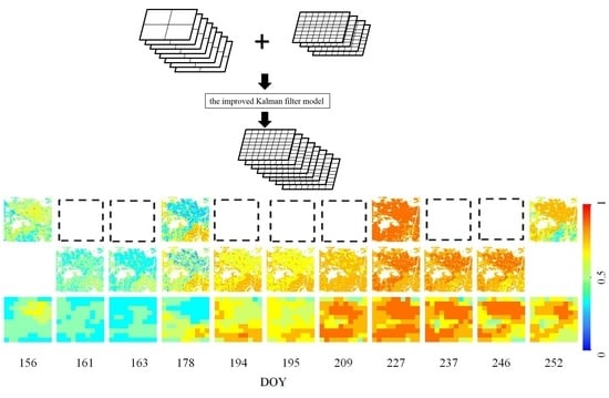
:Continuous monitoring of crop growth status using time-series remote sensing image is essential for crop management and yield prediction. The growing season of summer corn in the North China Plain with the period of rain and hot, which makes the acquisition of cloud-free satellite imagery very difficult. Therefore, we focused on developing image datasets with both a high temporal resolution and medium spatial resolution by harmonizing the time-series of MOD09GA Normalized Difference Vegetation Index (NDVI) images and 30-m-resolution GF-1 WFV images using the improved Kalman filter model. The harmonized images, GF-1 images, and Landsat 8 images were then combined and used to monitor the summer corn growth from 5th June to 6th October, 2014, in three counties of Hebei Province, China, in conjunction with meteorological data and MODIS Evapotranspiration Data Set. The prediction residuals () in NDVI between the GF-1 observations and the harmonized images was in the range of −0.2 to 0.2 with Gauss distribution. Moreover, the obtained phenological curves manifested distinctive growth features for summer corn at field scales. Changes in NDVI over time were more effectively evaluated and represented corn growth trends, when considered in conjunction with meteorological data and MODIS Evapotranspiration Data Set. We observed that the NDVI of summer corn showed a process of first decreasing and then rising in the early growing stage and discuss how the temperature and moisture of the environment changed with the growth stage. The study demonstrated that the synthesized dataset constructed using this methodology was highly accurate, with high temporal resolution and medium spatial resolution and it was possible to harmonize multi-source remote sensing imagery by the improved Kalman filter for long-term field monitoring.
1. Introduction
Local climate and local crop management strategies are important factors that determine crop yield in a given area. Light, heat, and water are necessary for the photosynthesis of crops, and farmers can intervene in farmland appropriately according to crop growth needs [1]. Continuous monitoring of crop growth and environmental changes is of great significance for crop management and yield estimation [2]. Time-series remote sensing images from satellites are important data sources for monitoring crop growth.
For long-term vegetation monitoring targets, the images with high temporal resolution and low spatial resolution, e.g., MODIS and AVHRR, are one of the preferred data sources [3,4]. The MODIS synthesized vegetation index products have many applications in monitoring global climate change, material and energy cycles and the growth of surface vegetation. Guindin-Garcia et al. [5] integrated the MODIS eight-day and 16-day products to quantitatively estimate green leaf area index (GLAI) over corn fields and evaluate the potential and limitations of the satellite data. Doraiswamy et al. [6] evaluated the applicability of the eight-day MODIS composite imagery in monitoring crop growth and yield estimation and the results showed that these images were very reliable. Sakamoto et al. [7,8] proposed a method which could identify the growth period of maize and soybean with two-step filtering based on MODIS data. However, the low spatial resolution (i.e., 250 m or 500 m) will cause a lot of errors by mixing multiple objects which have great differences in spectral curves and phenological characteristics in one pixel. Wang et al. [9] monitored and evaluated the growth condition of spring maize based on MODIS vegetation index products, MODIS LAI products and Global Land Surface Satellites LAI product. Moreover, the medium-resolution satellites (i.e., Landsat and GF-1) have developed rapidly and can well express the detailed features of the surface [10,11,12]. If the time-series is complete enough, the medium-resolution satellites can reflect the growth status of crops over the whole growing period. Due to both the low temporal resolution and because most crops grow during periods of high rainfall and heat, including the summer corn planted in eastern China, the quality of the images obtained during that period can be reduced due to clouds and smog. It also leads to the difficulty of obtaining high quality time series images even for satellites with higher temporal resolution, such as GF-1(four-day and 16 m). Most satellites cannot take high temporal resolution and high spatial resolution imagery at the same time, e.g., MODIS (daily and 500 m) and Landsat-8 (16-day and 30 m); therefore, it is difficult to obtain complete high-quality time-series image datasets from a single sensor covering the whole growing season of summer corn in China.
Spatiotemporal image fusion is one of the most effective ways to solve this problem [13,14]. The spatiotemporal image fusion method combines the characteristics of high temporal resolution images with high spatial resolution images, which facilitates the characterization of the details of the land surface being surveyed. The method can also help to resolve apparent contradictions between high temporal resolution and high spatial resolution imagery datasets [15]. Spatiotemporal remote sensing image fusion is a practical and low-cost method. It not only utilizes remote sensing images with high temporal and spatial resolutions, but also promotes the utilization of current earth observation data [16].
Spatiotemporal data fusion based on machine learning is one notable algorithmic method that has shown potential in recent years [17]. Sparse representation is used to realize super-resolution reconstruction of remote sensing images and enhance the spatial detail expression ability of low spatial resolution images which mainly used to improve the serious problem of mixed pixels in complex terrain coverage areas [18]. Yanovsky et al. [19] improved the resolution of microwave images based on sparse optimization and compressive sensing, and the research results showed that the data fusion products were better than all the statistical indicators of the original AMSU-B and AVHRR. Wang and Atkinson [20] designed the Fit-FC method, including regression model (RM) fitting, spatial filtering, residual compensation and fusion of Sentinel-2 (MSI) and Sentinel-3 (OLCI) images, to create approximately daily Sentinel-2 images. Using these advanced methods, super-resolution reconstructions of remote sensing images can be achieved, which enhances the resolution of low quality images and increases the detail of spatial expression. This is mainly used to resolve the serious problems of mixed pixel types in areas with complex terrain [21].
Gao et al. [22] introduced the spatial and temporal adaptive reflectance fusion Model (STARFM) method, which can blend MODIS and Landsat images for applications that require high resolution in both time and space. The STARFM model takes spatial variation and time variation information into account, and it is one of the most widely used space-time models. It is used in time series NDVI, LAI monitoring [23,24], estimation of regional evapotranspiration [25], ground surface temperature monitoring [26,27], and gross primary production (GPP) monitoring [28]. Other scholars [29,30,31,32,33,34] have improved the STARFM model based on Gao’s research. Among them, one of the most widely used is the ESTARFM algorithm, which is an enhanced spatial and temporal adaptive reflectance fusion model. The experimental results showed that ESTARFM [31] had a better prediction accuracy than STARFM. However, the ESTARFM model is sequentially input high time resolution data with high spatial resolution and high temporal resolution data and target during two periods, thereby generating high spatial resolution data of the target period. Thus, when the difference between the two moments is relatively large, the data generated during the target period will produce greater uncertainty.
Kalman filtering is a linear simulation and prediction algorithm that can be used for image fusion and for predicting new images. It provides a mathematical framework for predicting unmeasured variables from indirectly noisy measurements. As a predictive tool, Kalman filter is mainly used to estimate the state of dynamic systems, such as process control [35,36], flood forecasting [37], radar tracking [38], GNSS navigation [39,40] and performance analysis of estimation systems. Sedano et al. [41] used a Kalman filter algorithm to achieve spatiotemporal fusion of existing Landsat TM and 250-m NDVI MODIS (MOD13Q1) images for predictions of synthetic Landsat NDVI values. Huang et al. [42,43,44,45] used a Kalman filter algorithm to produce a 30-m-resolution LAI time-series, with a 4-day time-step using the Landsat TM LAI data and the S-G filtered MODIS LAI time-series. They then applied the 30-m-resolution LAI time series to model crop growth. Using the methods described in the references above, the Kalman filter can be applied using basic parameters, and it has the flexibility of being independent of the number of medium-resolution images obtained. The Kalman filtering algorithm uses a linear relationship to represent the time update of images, and considers the relationship between the image of the target and its forward and backward time by recursive algorithm. Nonetheless, the lack of observation data in the target period will lead to large errors in the measurement update.
Fortunately, the ESTARFM model is good at producing the details of observation data [15,31]. Therefore, we improved the Kalman filtering algorithm using the observation data producing operator of ESTARFM model, where the input of the images was generated by the ESTARFM model as an observation into the Kalman filtering algorithm. The harmonized image datasets with high temporal resolution same to MODIS image and medium spatial resolution (30 m) were produced using the improved Kalman filtering model by harmonizing GF-1 WFV images and Landsat 8 OLI images. The growth condition of summer corn from 5 June to 6 October 2014 was then analyzed in combination with meteorological data and evapotranspiration (ET) and latent heat flux (LE) data. The target of this research is to evaluate the potential and practicality of harmonizing multi-source remote sensing images using the improved Kalman filtering model and applying it to the crop growth monitoring.
2. Materials and Methods
2.1. Study Area
The study area is located in Zhuozhou, Gaobeidian and Dingxing County of Baoding City, Hebei Province, China, which ranges from 115°29′E, 39°5′N to 116°24′E, 39°35′N, as shown in Figure 1. This area is located in the North China Plain and has a temperate continental monsoon climate. The average annual temperature is approximately 9 °C–15 °C, the annual solar availability rate is approximately 60%, the annual precipitation is about 550 mm, and the water and heat conditions are suitable for growing crops. Corn and winter wheat are the main crops; others include soybean and cotton.
The summer corn is mostly planted before the winter wheat is harvested in the study area. Generally, the summer corn emerges in mid-June, and this is also the harvesting time of winter wheat. It enters the jointing stage in the early July, and enters the heading stage in the early August. From the late August to early September, it enters the milk-ripening period, and reaching the maturity stage in the middle of September [46,47,48]. This is the whole phenological period of summer corn in the study area, which is used to determine the time ranging of acquisition dates for multi-source remote sensing images.
2.2. Data Sources and Preprocessing
GF-1 was the first satellite of China’s high-resolution earth observation system and was successfully launched on 26 April 2013. The spatial resolution of GF-1 WFV images is 16 m, including four bands of blue, green, red and near-infrared, with revisiting period of four days. The GF-1 WFV images were downloaded from the China Centre for Resources Satellite Data and Application website (http://www.cresda.com/EN/). The acquisition dates of studied GF-1 images were shown in Figure 2. Effected by the cloud, smog and raining, only eight GF-1 WFV images were available here in the whole corn growing period.
Landsat 8 was successfully launched by NASA on 11 February 2013. This image could be downloaded freely from the USGS EarthExplorer website (http://earthexplorer.usgs.gov/). The imaging coverage size is 185 km by 185 km, with the revisiting period of 16 days. The published data indicate L1T and can be geometrically corrected for terrain form. In general, the datasets can be used directly without geometric correction. The preprocessing of GF-1 and Landsat 8 images included georeferencing, radiometric calibration, atmospheric correction, resampling and masking, which was done using the ENVI® v.5.2 software package (Exelis VIS, Boulder, CO, USA). First, radiometric calibration and atmospheric correction were done using FLAASH algorithm of ENVI® v.5.2. Then, the GF-1 images were georeferenced with Landsat 8 as the base map, with a resultant error of less than one pixel. Finally, the spatial resolution of the GF-1 images were resampled to 30 m using the nearest neighbor method and the datasets were cut down to represent only the research area.
MODIS is an important optical sensor for observing global biological and physical processes. MODIS sensors were carried on the sun-synchronous polar orbit satellites Terra and Aqua, which were successfully launched in 1999 and 2002, respectively. The MOD09GA reflectance product and MODIS Evapotranspiration Data Set (MOD16) [49,50] were used in this study. For the MOD09GA, there were seven bands ranging within blue, green, red, and near-infrared wavelengths at 459–479 nm, 545–565 nm, 620–670 nm, and 841–876 nm, similar to the band ranging of GF-1 images. There were 11 MODIS reflectance images in total in the whole corn growing season in the study area which were taken simultaneously on DOY 156, DOY 178, DOY 227, and DOY 252 with GF-1 images. For the MOD16, global evapotranspiration (ET) and latent heat flux (LE) datasets which we used were regular 1 km2 land surface ET datasets for the global vegetated land areas at 8-day. Notice that, the 8-day ET data (mm/8 day) is the sum of ET during these 8-day time periods, and the 8-day LE data (104 J/m2/day) is the average daily LE over the corresponding time period [51]. The downloaded MODIS images are preprocessed using MRT (MODIS Reprojection Tool) tool. First, the data are organized using a consistent day-numbering system. Then, the image sine projection format is converted to UTM 50N, for which the geographic coordinate system selected is WGS84. The output pixel size is 500 m by 500 m, and the “nearest neighbor” algorithm method was selected for downscaling to 30 m. A suitable cutting range for the study area was set, and the images were saved in GeoTIFF format. Finally, the files were saved with the above property settings, *.prm files were generated, and the command line was called to achieve data batch processing.
The meteorological datasets and LAI data were collected from 20 National Agrometeorological Observation Stations in Hebei Province. These automated weather stations were installed for long-term climate observation and provided data on daily maximum, minimum, and average temperatures, as well as daily precipitation. As can be seen from Figure 1, meteorological datasets are single-point datasets, and all of the stations lie outside the study area, so the data need to be spatially processed. In this study, we used the Kriging method to produce a dataset with a spatial resolution of 30 m by 30 m from the agrometeorological station data. Then, the average value of the data in the study area was calculated, including daily maximum, minimum, average temperatures, and daily precipitation. The LAI measurements were carried out on 10 samples of summer corn in the study area in the DOY 205 and DOY 224, which corresponded to the flare opening stage and the tasseling and anthesis silking of summer corn, respectively.
2.3. The Improved Kalman Filter
The Kalman filter method is a linear fitting and prediction algorithm. It was published in the “Journal of Basic Engineering Transactions” by Kalman in 1960 [52]. It can combine information from observational systems and system modeling to minimize residual errors and produce more accurate predictive information [53]. The method consists of three hypotheses: (i) the posterior probability obeys a Gaussian distribution; (ii) the system is linear; and (iii) both the system noise and the measurement noise are subject to Gaussian distribution. The method is described in Equations (1) and (2):
where and are the estimated values of the current state k and the previous state k − 1 of the model, respectively. For image harmonizing, and are the reflectance images on time k and k − 1 respectively (Figure 3). The connection of time k and k − 1 is done by state-transition matrix A, and the observed value is linearly related to the current state estimation . In addition, H is a measurement sensitivity matrix, are process noise N(0,Q) and measurement noise N(0,R), both of which obey a Gaussian distribution.
The Kalman filter is applied in two steps: the time update and the measurement update. In the time update, the state-transition matrix A can be represented in linear regression. The linear regression is used to describe the phenological trajectory between two moments, which can be represented by linear equations. In this paper, 211 sampling plots were selected within the images. Based on these plots, a linear relationship between the k−1 state and the k state of MODIS data was established, as shown in Equation (3). The slope and intercept of the linear regression line modeled a and b, respectively, which were used to transfer the prior estimation of the time change trend. The process noise is calculated by weighted standard error, and the weight is residual error. The uncertainty of the time update is calculated by Equation (4).
In the measurement update, a posteriori estimate value of the k state is calculated from the weighted sum of the observed value and prior estimate , as shown in Equation (5). The weights are defined as Kalman gain and are updated by uncertainty . is the measurement noise covariance matrix, and T represents the matrix transposition operation, as in Equations (6) and (7).
For the Kalman filter algorithm, it is vital to update the a priori estimate for the current point-in-time to obtain a posteriori estimate. Unfortunately, there are generally insufficient observation data resulting from cloud, smog and raining, etc. To solve this problem, there are usually two solutions: one is to use the posterior estimation of the previous moment, which is suitable for the case of small interval between two moments; the other is to use the low spatial resolution image of the current moment instead. Obviously, the two methods will produce more uncertainty for image harmonization. Therefore, we developed the improved Kalman filter by carrying out a priori estimate for the studied point-in-time using ESTARFM model for the NDVI images. NDVI is the combination of red band and NIR band reflectance, aiming at enhancing the difference between vegetation and non-vegetation [54,55]. During this process, we first calculated the NDVI products based on the preprocessed reflectance images, including GF-1 images and MODIS images. Secondly, we used the NDVI products of MODIS images and GF-1 images to generate a set of 30-m resolution observation data () using ESTARFM model. Finally, the time trajectory of time series MODIS NDVI (sub-model 1) and the updated observation data resulting from ESTARFM model (sub-model 2) were used to harmonize GF-1 images and MODIS images.
The main idea of updating the observation data for studied point-in-time using ESTARFM model is to establish the correlation of the two resolution images and to minimize the systematic error. The ESTARFM algorithm code which we used in this study is from Zhu [31] and the download address is (https://xiaolinzhu.weebly.com/open-source-code.html). The algorithm uses mobile windows, which size is and determines the predicted values of moving pixels in the center at state. It can be calculated as follows, according to Equation (8):
where is the central pixel, and the represents the image bands. and represent the fine-resolution data at i and ii state which is integrated by similar pixels in the moving window as Equation (9). and are time weight of state and as Equation (10). In these equations, we default that < < .
where expresses the low temporal resolution and high spatial resolution images, and expresses the high temporal resolution and low spatial resolution images, the value of I is i and ii, is the number of and similar pixels embrace the central pixel, and is the location of the jth similar pixel, and represent the weight and the conversion coefficient of the jth similar pixel, respectively. The algorithm flow of the improved Kalman filter is shown in the Figure 3.
The Kalman filtering algorithm is a recursive algorithm, which can perform forward filtering and backward filtering . For the state k, the weighted sum of forward filtering and backward filtering can improve the reliability of a posteriori estimation, and weights are calculated from forward uncertainty and backward uncertainty , as shown in Equations (11) and (12):
2.4. Accuracy Assessment of Image Harmonizing
In this study, we used two observation images (DOY 178 and DOY 227) to verify the accuracy of the model. Owing to these two images were not involved in image harmonizing process, the verification observation data and synthetic data were independent of each other. We compared the NDVI images observed by satellite with the harmonized NDVI images, and calculated the prediction residuals () of each pair of images to evaluate the accuracy of the fused images. The prediction residual images of ESTARFM model and improved Kalman filtering model and their probability density images were analyzed to evaluate the ability of the two models to fuse data. The prediction residual was computed as:
where is the prediction residual at pixel level, is the pixel value in the observation image, and is the pixel value of harmonized image. The improved Kalman filter model and the data analysis algorithms were running under MATLAB (The Mathworks, Inc., Natick, MA, USA) environment.
3. Results and Analysis
3.1. Accuracy Assessment Results of Image Harmonizing
The spatiotemporal fusion of images using the improved Kalman filter preserves the high temporal resolution of low spatial resolution images, but the product results also inherits high spatial resolution characteristics. The spatial resolution of the harmonized images is 30 m, and the temporal resolution is determined by the time interval of the MODIS source images. For example, if all MOD09GA images are available, then the temporal resolution of the harmonized images is daily.
Similar spatial details can be used to evaluate qualitatively the accuracy of image harmonizing using the improved Kalman filter, and temporal variation trends can be obtained. To reveal the spatial details of harmonized image clearly, we chose a farmland with an area of about 5000 m × 5000 m, as shown in Figure 4a–e, which is consist of farmland (about 75%), residential areas (about 20%) and other areas (about 5%).
The Figure 5 represents spatial values for the NDVI calculated using GF-1 image, MODIS image and harmonized image, respectively. As it can be seen from Figure 5, there are only four image pairs of GF-1 image and MODIS image on DOY 156, DOY 178, DOY 227 and DOY 252. Excepting for these four image acquisition dates, there are seven MODIS images without simultaneous collected GF-1 images. In order to verify the accuracy of spatiotemporal fusion model, the image acquired on DOY 178 and DOY 227 are not used for image harmonizing, and only for assessing the image harmonizing accuracy. Figure 5 shows that the harmonized images on DOY 156, DOY 178, DOY 227 and DOY 252 have a similar spatial variation pattern with the simultaneous MODIS images, visually. Moreover, the harmonized images on DOY 178 and DOY 227 have very similar spatial details with the simultaneous GF-1 images. These two similarities reveal the harmonized images carry on the time trajectory of MODIS time-series images and detailed spatial specifics of GF-1 images. From the time-series harmonized images and MODIS images, the corn phenological growing changes in the study area can be inferred clearly. NDVI shows a tendency to increase slowly at early growing stage, and change to increase quickly at the middle growing stage, and then decrease slowly at the end of growing stage. From the zoomed time-series images, we can see that the phenological changes are basically consistent for the harmonized images and MODIS images.
Normally, the NDVI values with the maximum probability density can show the temporal and spatial variations and differences for studied summer corn more clearly, because they represent the overwhelming majority of summer corn plants growing condition. Figure 6 shows the time series of NDVI value with the maximum probability density resulting from time-series GF-1 images, harmonized images and MODIS images. Specifically, the NDVI value with the maximum probability density generally ranges from 0 to 0.5 before DOY 163, and increases to around 0.5 on the DOY 178, and increases to a range from 0.6 to 0.9 on DOY 194. Moreover, there are two peaks for the probability density distribution of NDVI values of GF-1 and harmonized images on DOY 227, with one lower peak around 0.4 and another higher peak around 0.8. Unfortunately, the time-series MODIS images show a single peak only, which cannot capture this little spectral variation. This comparation reveals that the harmonized images can carry on the fine spatial resolution of the GF-1 images. Another comparation is about the difference of three maximum probability density curves of GF-1, MODIS and harmonized images on DOY 178 shown in Figure 6. The mean NDVI value of three maximum probability density functions are all around 0.5. However, the maximum probability values of them are 3.9, 6.2 and 4.9 for GF-1 image, MODIS image and harmonized image, respectively. This indicates that the harmonized images can carry on the fine spatial resolution of the GF-1 images. In terms of the range of NDVI values, it is obvious that the ranges of GF-1 and harmonized images are broader than MODIS image, which reveal that there is a finer spatial detail expression ability in low vegetation coverage area and high vegetation coverage area on GF-1 image and harmonized image than on the MODIS image.
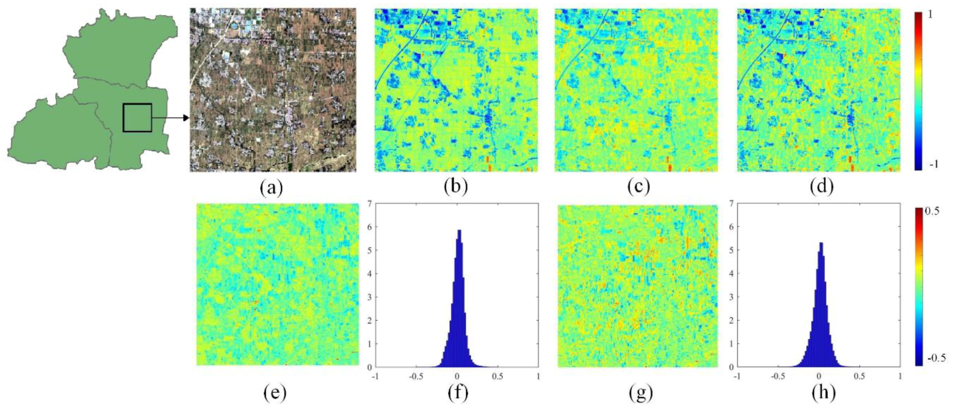
Figure 7 and Figure 8 show the spatial details of NDVI pattern for GF-1 image, MODIS image and harmonized image on DOY 178 and DOY 227, respectively. Figure 7a and Figure 8a indicate the position of zoomed subset areas for analyzing of NDVI pattern on DOY 178 and DOY 227. Figure 7b–d are the NDVI calculated from harmonized image using the improved Kalman filter, the original GF-1 NDVI images, the harmonized image using ESTARFM model respectively. We can see that from Figure 7b–d, there is a similar NDVI spatial variation pattern on harmonized images (Figure 7b,d) with the original GF-1 NDVI images (Figure 7c), northwest of this zoomed area is lower than other regions. This reveals that the harmonized images carry on the spatial details of the original GF-1 NDVI images. Figure 7e,g are the between the original GF-1 NDVI images (Figure 7c) and harmonized images using the improved Kalman filter (Figure 7b) and ESTARFM model (Figure 7d) respectively. We can see that the NDVI of harmonized images using the improved Kalman filter are higher in vegetation area than that in the original GF-1 NDVI images (negative difference value), lower in non-vegetation area (positive difference value). Diversely, the NDVI of harmonized images using ESTARFM model are mostly higher than GF-1 image (negative difference value) in the whole zoomed area. In addition, Figure 7f shows that the ranging between harmonized images using the improved Kalman filter and the original GF-1 NDVI images is −0.2~0.2. Figure 7h shows the ranging between harmonized images using ESTARFM model and the original GF-1 NDVI images is −0.25~0.25. This reveals that the harmonizing accuracy using improved Kalman filter is higher than that using ESTARFM model. Similar conclusions can be obtained by Figure 8.
Furthermore, the quantitative assessment is done to validate the image harmonizing accuracy using the improved Kalman filter and ESTARFM model. Figure 5 shows that there are four GF-1 high spatial resolution images used for the time series images harmonizing, which are acquired on DOY 156, DOY 178, DOY 227 and DOY 252 respectively. There are only two image pairs that there are simultaneous GF-1 image, harmonized image and MODIS image on DOY 178 and DOY 227.
In order to verify the accuracy of the improved Kalman filter, the image acquired on DOY 178 and DOY 227 are not used in time-series image harmonizing, which are used only for image harmonizing accuracy assessment in this study. If these two images are used for practical image harmonizing, the accuracy of which will be higher than the accuracy results listed in Table 1. As it can be seen from Table 1, the image harmonizing accuracy using the improved Kalman filter is higher than that using the ESTARFM model in DOY 178 and DOY 227. For the harmonized image on DOY 178, the coefficient of determination (R2) between the harmonized image using the improved Kalman filter and GF-1 image is 0.65, which is higher than the harmonized image using ESTARFM model (R2 = 0.55). Moreover, the root mean square error (RMSE) of the improved Kalman filter (RMSE = 0.08) is lower than that of the ESTARFM model (RMSE = 0.09). Similarly, the harmonizing accuracy on the DOY 227 using the improved Kalman filter is higher (with R2 = 0.84, RMSE = 0.07) than that using ESTARFM model (R2 = 0.82, RMSE = 0.08).
3.2. Summer Corn Growth Mornitoring Results Using Harmonized Time-Deries Images
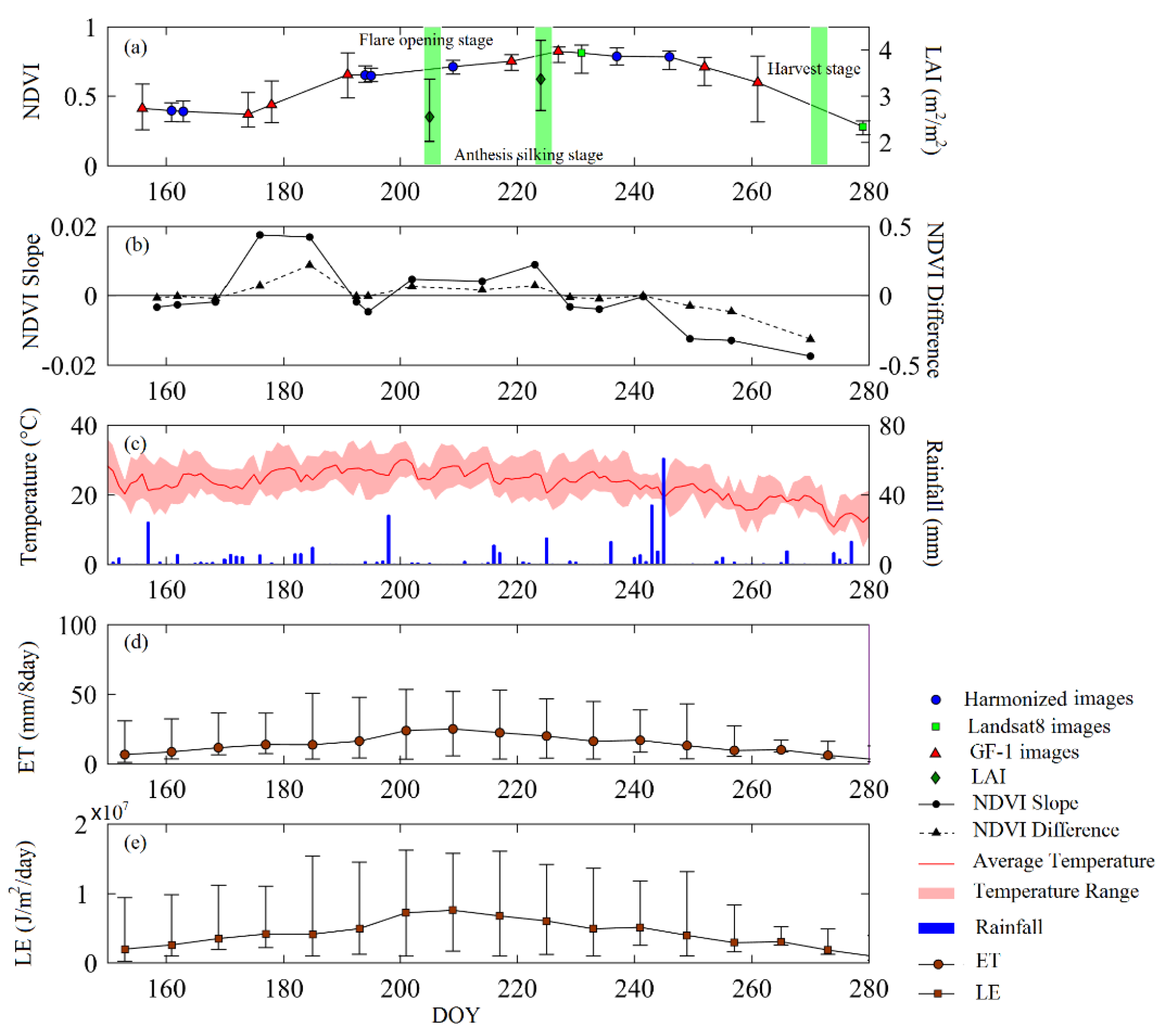
The harmonized time-series remote sensing images are the very ideal data source for summer corn growth monitoring because the growth difference can be reflected on the spectral variation and difference. In this study, we monitored the summer corn growth condition and changing using time-series NDVIs from harmonized images. Moreover, the MODIS ET and LE products (MOD16) and meteorological data (rainfall, temperature in the corn growing season) were combined to analyse the summer corn growth behavior, in other words, how the summer corn growth status (i.e. NDVI) change with the change of rainfall, temperature and evapotranspiration. The time-series NDVI changing curve from DOY 156 to DOY 252 is used to analysis the summer corn growing and changing in study area. In addition, the changing slope and difference between neighboring NDVIs are calculated and used to quantize the summer corn growing and changing. The changing slope and difference of NDVI curve are calculated as follows:
Figure 9 is changing curve of time-series NDVI from harmonized remote sensing images over the summer corn fields. In addition, the simultaneous rainfall and daily temperature change curves from DOY 156 to DOY 252 are compared and analyzed synchronously. In study area, an interplanting system of winter wheat and summer corn was implemented in the study area to ensure two crops each year. From DOY 156 to DOY 174, the winter wheat was in the mature stage, while the summer corn was in the seeding and emergence stage. On DOY 156, the average rainfall was 1.4 mm, and the ET reaches 6.5 mm/8 day and LE reaches 2 × 10⁶ J/m2/day. From DOY 156 to DOY 174, the temperature increased continually, of which the average highest temperature during the day reached 29.8 °C, with an average temperature of 23.4 °C. The winter wheat began to turn yellow and dry, so the NDVI decreased and the slope value was therefore less than 0.
From DOY 174 to DOY 195, the summer corn is in the jointing stage. During this period, the average rainfall was 2.8 mm. The rainfall on DOY 164 and DOY 196 was 0.08 mm and 1.17 mm, respectively. So the ET and LE increased continually. The temperature continued to increase, and the average highest temperature during the day reached 32.6 °C, with an average temperature of 26.5 °C. At this time, the climatic condition is favorable for the rapid growth of corn leaves. Therefore, the NDVI increased rapidly and the slope values and differences are all greater than 0.
From DOY 196 to DOY 227, the summer corn is in the heading stage. During this period, the average rainfall is 2.3 mm and the temperature continued to be in a higher range. The average highest temperature during the day reached 31.9 °C, with an average temperature of 26.0 °C. The water content in the vegetation increased, and the ET increase its maximum level from 16.1 to 24.9 mm/8 day and LE increase from 4.9 to 7.6 × 10⁶ J/m2/day, then they gradually decreased. Especially, there was an obvious rainfall and warming process on the DOY 198 to DOY 200 where the rainfall reached 28 mm and the average temperature increased by 5 °C. Likewise, the ET and LE increased rapidly from DOY 193 to DOY 201. It shows that the MOD16 product has high accuracy, which could reflect the changes of ET and LE on a regional scale, but also shows that the ET and LE are closely related to precipitation and temperature. The NDVI reached the maximum in the whole growing stage. The slope value and the difference were all greater than 0. However, it could be seen from the diagram that the NDVI gradient from DOY191–194 to DOY 194–195 NDVI is negative, indicating a small decrease in NDVI. The reason for this variation may be that the time difference between the three images is very small, and the influence of errors is therefore larger. We concluded that this stage was the key stage of high growth rate of summer maize. The LAI measured on the ground showed that the average LAI value increased from 2.5 (DOY 205, flare opening stage) to 3.4 m2/m2 (DOY 224, tasseling and anthesis silking).
From DOY 227 to DOY 246, the summer corn is in the milking stage, and it needs a larger leaf area for photosynthesis to transform the organic matter into corn grain. The photosynthesis of corn leaves depends on the adequate availability of suitable light, heat, and water. During this period, the precipitation in the study area reached the peak value, which averaged 6.8 mm, and the ET and LE are still at a higher stage but they are gradually decreasing. At the same time, the average highest temperature reached during the day was 29.4 °C, with an average temperature of 23.5 °C, and the day and night temperature difference was greater than 10 °C. These factors are beneficial to photosynthesis and the transformation of organic matter; therefore, the leaf area of the corn remained in a larger range. On the DOY 241, a continuous rainfall process can be seen, but at this point the temperature decreased. Then, the ET is increased by 1 mm/8 day and LE is increased by 2 × 10⁵ J/m2/day.
From DOY 246 to DOY 279, the summer corn was in the ripening stage. During this growing stage, the dry matter accumulation process of summer corn almost stopped, and the dry weight of the grains reached their maximum. Precipitation began to decline, the average precipitation dropped to 1.2 mm, the vegetation began to lose water, and the ET and LE also descended. The temperature and evaporation rates were reduced, and the average highest temperature during the day reached 23.7 °C, with an average temperature of 17.9 °C. The corn leaves began to turn yellow, leaf area decreased, and NDVI began to decline rapidly. The slope and differences were all below 0.
From this time-series diagram, we can see that the summer corn grows quickly with the quick increasing NDVI at early growing stage, stable in the middle growing stage and decreases in the late growing stage. Moreover, the NDVI, ET and LE all increase after the rainfall in the early growing stage. Generally, this delay would be four to five days.
4. Discussion
4.1. The Improved Kalman Filter Model
Kalman filter is an algorithm for optimal estimation of system state which uses linear equation of system state and observation data. When we predicted the missing GF-1 image by Kalman filter, we found that the model was uncertain due to the lack of observation value. Consequently, we generated a set of observation data, firstly through ESTARFM model and applied it to Kalman filter. In our work, the result manifested that the improved Kalman filter had good performance in predicting GF-1 images. As shown in Figure 5, the harmonized images using improved Kalman filter depicted the growing and changing of summer corn well, and was in good agreement with the temporal changing curve of MODIS images which had a low spatial resolution. Importantly, compared with the ESTARFM model, the improved Kalman filter added the function of filtering on time series, and through the forward and backward filtering of Kalman filter, the weighted average was carried out according to the uncertainty to achieve a smooth effect. We used the real observations (DOY 178 and DOY 227) which were not involved in synthesis as validation data. As could be seen from the Figure 7 and Figure 8, the synthesized dataset constructed using this methodology was highly accurate, with high temporal resolution and medium spatial resolution.
Although there are important discoveries revealed by our studies, there are also limitations. First, the problem of missing data due to weather (e.g., clouds, raining and smog) has not been thoroughly solved. In spite of the synthesis algorithm based on multi-source data platform alleviates this problem to some extent, it is possible to not get an image for a month. Especially in our research area, this phenomenon is particularly serious. Chen et al. [56] compared four kinds of image fusion methods, including ESTARFM, and showed that the ESTARFM performed more stably than other models. However, the results of Walker et al. [57,58] showed that MODIS 8-day composite datasets had more acceptable correlations for distinguishing phenology variations at shorter time frames than 16-days. Long time intervals will lead to large changes in vegetation cover and NDVI due to vegetation growth, which will have a negative impact on the quality of the predicted image. To some extent, the improved Kalman filter alleviates this contradiction, but it cannot be ignored. Second, the BRDF effect of MODIS images also has a beneficial effect on the results. Kim et al. [59] reminded of the BRDF effects in MODIS images can be considerable because of the large swath width. In practice, we used NDVI to reduce the BRDF effect. Furthermore, the selection of sampling plots was done manually, which greatly reduces the image processing ability. The meaning of Equation (3) is to capture the changes of vegetation growth over time on existing low-resolution images and use it to predict the high-resolution prior estimation at the next moment. Therefore, the selection of quadrats is very important as it requires pure corn pixels. Huang et al. [44] pointed out that the higher pixel purity could improve the accuracy of LAI of time series and crop yield estimation. We selected relatively pure corn pixels manually according to land-use classification data (excluding those cloudy and serious mixed pixels). The process of manual selection was time-consuming and laborious, which greatly reduced the efficiency of the algorithm.
In the future, we will try to introduce Synthetic Aperture Radar (SAR), which is not affected by weather conditions such as clouds and rain into the improved Kalman filter model and develop an automatic method to select sampling plots.
4.2. Application Potential of Crop Growth Process Monitoring
Corn is an important grain crop in North China Plain. According to planting time and variety, corn can be roughly divided into spring corn and summer corn. In the two-year three-cropping area, the planting area of summer corn is much larger than that of spring corn. The growing season of summer corn is from June to October. The rainy season is in July and August, and it is also the key period of maize growth, which is closely related to the final yield. The lack of clear sky observations from optical satellite due to weather factors such as clouds and smog is widespread in other agricultural regions of China [60]. Because of the shortcomings of temporal resolution or spatial resolution, single sensor remote sensing satellite cannot satisfy the requirement of long-term monitoring of crop accurately. It is one of the important methods for crop growth monitoring in the field scale based on time-series spatial-temporal fusion images harmonized by multi-source remote sensing data sources.
Previous studies [2,9,26,41] have demonstrated that the availability and great potential of long time series remote sensing images in crop growth monitoring. In this paper, the result manifested that the improved Kalman filter could be used to harmonize the time-series multi-source remote sensing images for summer corn growth monitoring. Finally, we analyzed the growth situation of summer corn in the study area based on NDVI time-series dataset synthesized from multi-source remote sensing data and discussed how the temperature and moisture of the environment changed with the growth stage. The growth process of summer corn obtained from synthetic remote sensing images could be directly applied to follow-up studies, such as precise farmland management of irrigation, fertilization and pesticides and yield estimation over large areas. Furthermore, our results suggested that the application potential of synthesizing multi-source data in crop growth monitoring is enormous and it was a low-cost method to obtain complete time-series images in the field scale at the present stage.
5. Conclusions
This paper presented a method for monitoring summer corn crop growth by harmonizing multi-source remote sensing images. We harmonized the high spatial and temporal resolution images using improved Kalman filter based on daily MOD09GA reflectance images with the 250 m spatial resolution and GF-1 WFV images with 30-m-resolution. The growth status of summer corn in a designated research area was analyzed during part of 2014 in conjunction with MOD16 ET and LE product and meteorological data.
We were able to draw a number of conclusions from our research. First, the high temporal and spatial resolution images reconstructed using the improved Kalman filter had higher precision than ESTARFM model only; it not only inherited the phenological trends in the MODIS data, but also preserved the spatial detail levels of the GF-1 datasets; moreover, the prediction accuracy of satellite images after corn silking is higher than that of early stage. Second, the vegetation indexes calculated from the multi-source image datasets, including NDVI, can be used to monitor the growth of crops at all stages when the analysis is combined with MOD16 ET and LE product and meteorological data. This includes slope and differences calculated from NDVI values. Third, before the milking stage, NDVI values for summer corn increased with the increase of temperature and precipitation. After the milking stage, NDVI first stabilized for a period of time and then decreased with the decrease of temperature and precipitation. The ET and LE data had a close relationship with the temperature and precipitation data.
In conclusion, the harmonized multi-source remote sensing datasets can effectively reflect crop growth. The improved Kalman filter model can help resolve issues arising from incomplete satellite imaging datasets, particularly in areas with adverse climatic conditions. This monitoring method should be applied to other crops and to a broader range of source data, including that associated with diseases, insect pests, and final crop yield totals, in the future.
Author Contributions
Conceptualization, M.Z., W.S. and J.H.; methodology, W.S. and M.Z.; software, M.Z. and D.Z.; writing—original draft preparation, M.Z. and W.S.; writing—review and editing, X.Z. and Z.L.
Funding
This study was funded by the National Natural Science Foundation of China under the project “Growth process monitoring of corn by combining time series spectral remote sensing images and terrestrial laser scanning data” (No. 41671433) and “Estimating the leaf area index of corn in whole growth period using terrestrial LiDAR data” (No. 41371327), Chinese Universities Scientific Fund “Monitoring the quantity and quality using remote sensing and intelligence analysis of total factor for cropland” (No. 2019TC117) and “Retrieval of biomass for summer corn after canopy is closed using remote sensing image” (No. 2019TC138) and Science and Technology Facilities Council of UK- Newton Agritech Programme (Project No. ST/N006798/1).
Acknowledgments
We thank the journal’s editors and anonymous reviewers for their kind comments and valuable suggestions to improve the quality of this paper.
Conflicts of Interest
The authors declare no conflict of interest.
References
- Franch, B.; Vermote, E.; Becker-Reshef, I.; Claverie, M.; Huang, J.; Zhang, J.; Justice, C.; Sobrino, J. Improving Timeliness of Winter Wheat Production Forecast in United States of America, Ukraine and China Using MODIS Data and NCAR Growing Degree Day. Remote Sens. Environ. 2015, 161, 131–148. [Google Scholar] [CrossRef]
- Gao, F.; Hilker, T.; Zhu, X.; Anderson, M.; Masek, J.; Wang, P.; Yang, Y. Fusing Landsat and MODIS Data for Vegetation Monitoring. IEEE Geosci. Remote Sens. Mag. 2015, 3, 47–60. [Google Scholar] [CrossRef]
- JoNsson, P.; Eklundh, L. TIMESAT—A program for analyzing time-series of satellite sensor data. Comput. Geosci. 2004, 30, 833–845. [Google Scholar] [CrossRef]
- Walsh, S.J.; Davis, F.W. Applications of remote sensing and geographic information systems in vegetation science: Introduction. J. Veg. Sci. 1994, 5, 609–614. [Google Scholar] [CrossRef]
- Guindin-Garcia, N.; Gitelson, A.A.; Arkebauer, T.J.; Shanahan, J.; Weiss, A. An evaluation of modis 8- and 16-day composite products for monitoring maize green leaf area index. Agric. For. Meteorol. 2012, 161, 15–25. [Google Scholar] [CrossRef]
- Doraiswamy, P.C.; Hatfield, J.L.; Jackson, T.J.; Akhmedov, B.; Prueger, J.; Stern, A. Crop condition and yield simulations using landsat and modis. Remote Sens. Environ. 2004, 92, 548–559. [Google Scholar] [CrossRef]
- Sakamoto, T.; Wardlow, B.D.; Gitelson, A.A.; Verma, S.B.; Suyker, A.E.; Arkebauer, T.J. A two-step filtering approach for detecting maize and soybean phenology with time-series modis data. Remote Sens. Environ. 2010, 114, 2146–2159. [Google Scholar] [CrossRef]
- Sakamoto, T.; Gitelson, A.A.; Arkebauer, T.J. MODIS-based corn grain yield estimation model incorporating crop phenology information. Remote Sens. Environ. 2013, 131, 215–231. [Google Scholar] [CrossRef]
- Wang, P.; Zhou, Y.; Huo, Z.; Han, L.; Qiu, J.; Tan, Y.; Liu, D. Monitoring growth condition of spring maize in Northeast China using a process-based model. Int. J. Appl. Earth Obs. Geoinf. 2018, 66, 27–36. [Google Scholar] [CrossRef]
- Roy, D.; Wulder, M.; Loveland, T.; Woodcock, C.E.; Allen, R.; Anderson, M.; Helder, D.; Irons, J.R.; Johnson, D.; Kennedy, R.; et al. Landsat-8: Science and product vision for terrestrial global change research. Remote Sens. Environ. 2014, 145, 154–172. [Google Scholar] [CrossRef] [Green Version]
- Wu, M.; Zhang, X.; Huang, W.; Niu, Z.; Wang, C.; Li, W.; Hao, P. Reconstruction of daily 30 m data from HJ CCD, GF-1 WFV, Landsat, and MODIS data for crop monitoring. Remote Sens. 2015, 7, 16293–16314. [Google Scholar] [CrossRef]
- Boschetti, M.; Bocchi, S.; Brivio, P.A. Assessment of pasture production in the Italian Alps using spectrometric and remote sensing information. Agric. Ecosyst. Environ. 2007, 118, 267–272. [Google Scholar] [CrossRef]
- Jarihani, A.; McVicar, T.; Van Niel, T.; Emelyanova, I.; Callow, J.; Johansen, K. Blending Landsat and MODIS Data to Generate Multispectral Indices: A Comparison of “Index-then-Blend” and “Blend-then-Index” Approaches. Remote Sens. 2014, 6, 9213–9238. [Google Scholar] [CrossRef]
- Emelyanova, I.V.; McVicar, T.R.; Van Niel, T.G.; Li, L.T.; van Dijk, A.I.J.M. Assessing the accuracy of blending Landsat-MODIS surface reflectances in two landscapes with contrasting spatial and temporal dynamics: A framework for algorithm selection. Remote Sens. Environ. 2013, 133, 193–209. [Google Scholar] [CrossRef]
- Gao, F.; Anderson, M.C.; Zhang, X.; Yang, Z.; Alfieri, J.G.; Kustas, W.P.; Mueller, R.; Johnson, D.M.; Prueger, J.H. Toward mapping crop progress at field scales through fusion of Landsat and MODIS imagery. Remote Sens. Environ. 2017, 188, 9–25. [Google Scholar] [CrossRef] [Green Version]
- Huang, B.; Song, H. Spatiotemporal Reflectance Fusion via Sparse Representation. IEEE Trans. Geosci. Remote Sens. 2012, 50, 3707–3716. [Google Scholar] [CrossRef]
- Chen, X.; Liu, M.; Zhu, X.; Chen, J.; Zhong, Y.; Cao, X. “Blend-then-Index” or “Index-then-Blend”: A Theoretical Analysis for Generating High-resolution NDVI Time Series by STARFM. Photogramm. Eng. Remote Sens. 2018, 84, 65–73. [Google Scholar] [CrossRef]
- Yang, J.; Wright, J.; Huang, T.S.; Ma, Y. Image super-resolution via sparse representation. IEEE Trans. Image Process. 2010, 19, 2861–2873. [Google Scholar] [CrossRef]
- Yanovsky, I.; Behrangi, A.; Wen, Y.; Schreier, M.; Dang, V.; Lambrigtsen, B. Enhanced Resolution of Microwave Sounder Imagery through Fusion with Infrared Sensor Data. Remote Sens. 2017, 9, 1097. [Google Scholar] [CrossRef]
- Wang, Q.; Atkinson, P.M. Spatio-temporal fusion for daily Sentinel-2 image. Remote Sens. Environ. 2018, 204, 31–42. [Google Scholar] [CrossRef]
- Li, J.; Yuan, Q.; Shen, H.; Meng, X.; Zhang, L. Hyperspectral Image Super-Resolution by Spectral Mixture Analysis and Spatial–Spectral Group Sparsity. IEEE Geosci. Remote Sens. Lett. 2016, 13, 1250–1254. [Google Scholar] [CrossRef]
- Gao, F.; Masek, J.; Schwaller, M.; Hall, F. On the blending of the Landsat and MODIS surface reflectance: Predicting daily Landsat surface reflectance. IEEE Trans. Geosci. Remote Sens. 2006, 44, 2207–2218. [Google Scholar]
- Dong, T.; Liu, J.; Qian, B.; Zhao, T.; Shang, J. Estimating winter wheat biomass by assimilating leaf area index derived from fusion of Landsat-8 and MODIS data. Int. J. Appl. Earth Obs. Geoinf. 2016, 49, 63–74. [Google Scholar] [CrossRef]
- Houborg, R.; Mccabe, M.F.; Gao, F. A Spatio-Temporal Enhancement Method for medium resolution LAI (STEM-LAI). Int. J. Appl. Earth Obs. Geoinf. 2016, 47, 15–29. [Google Scholar] [CrossRef] [Green Version]
- Liu, K.; Chen, S.; Tian, J.; Li, X.; Wang, W.; Yang, L.; Liang, H. Assessing a scheme of spatial-temporal thermal remote-sensing sharpening for estimating regional evapotranspiration. Int. J. Remote Sens. 2018, 39, 3111–3137. [Google Scholar] [CrossRef]
- Shen, H.; Huang, L.; Zhang, L.; Wu, P.; Zeng, C. Long-term and fine-scale satellite monitoring of the urban heat island effect by the fusion of multi-temporal and multi-sensor remote sensed data: A 26-year case study of the city of Wuhan in China. Remote Sens. Environ. 2016, 172, 109–125. [Google Scholar] [CrossRef]
- Quan, J.; Zhan, W.; Ma, T.; Du, Y.; Guo, Z.; Qin, B. An integrated model for generating hourly Landsat-like land surface temperatures over heterogeneous landscapes. Remote Sens. Environ. 2018, 206, 403–423. [Google Scholar] [CrossRef]
- Singh, D. Generation and evaluation of gross primary productivity using Landsat data through blending with MODIS data. Int. J. Appl. Earth Obs. Geoinf. 2011, 13, 59–69. [Google Scholar] [CrossRef]
- Wu, M.; Huang, W.; Niu, Z.; Wang, C.; Li, W.; Yu, B. Validation of synthetic daily Landsat NDVI time series data generated by the improved spatial and temporal data fusion approach. Inf. Fusion. 2018, 40, 34–44. [Google Scholar] [CrossRef]
- Zhu, X.; Chen, J.; Gao, F.; Chen, X.; Masek, J. An enhanced spatial and temporal adaptive reflectance fusion model for complex heterogeneous regions. Remote Sens. Environ. 2010, 114, 2610–2623. [Google Scholar] [CrossRef]
- Zhang, H.K.; Huang, B.; Zhang, M.; Cao, K.; Yu, L. A generalization of spatial and temporal fusion methods for remotely sensed surface parameters. Int. J. Remote Sens. 2015, 36, 4411–4445. [Google Scholar] [CrossRef]
- Hilker, T.; Wulder, M.A.; Coops, N.C.; Linke, J.; Mcdermid, G.; Masek, J.; Gao, F.; White, J. A new data fusion model for high spatial- and temporal-resolution mapping of forest disturbance based on Landsat and MODIS. Remote Sens. Environ. 2009, 113, 1613–1627. [Google Scholar] [CrossRef]
- Gevaert, C.M.; García-Haro, F.J. A comparison of STARFM and an unmixing-based algorithm for Landsat and MODIS data fusion. Remote Sens. Environ. 2015, 156, 34–44. [Google Scholar] [CrossRef]
- Xie, D.; Zhang, J.; Zhu, X.; Pan, Y.; Liu, H.; Yuan, Z.; Yun, Y. An Improved STARFM with Help of an Unmixing-Based Method to Generate High Spatial and Temporal Resolution Remote Sensing Data in Complex Heterogeneous Regions. Sensors 2016, 16, 207. [Google Scholar] [CrossRef] [PubMed]
- Ebadollahi, S.; Saki, S. Wind Turbine Torque Oscillation Reduction Using Soft Switching Multiple Model Predictive Control Based on the Gap Metric and Kalman Filter Estimator. IEEE Trans. Ind. Electron. 2017, 65, 3890–3898. [Google Scholar] [CrossRef]
- Hu, J.; Xiong, R. Contact Force Estimation for Robot Manipulator Using Semiparametric Model and Disturbance Kalman Filter. IEEE Trans. Ind. Electron. 2018, 65, 3365–3375. [Google Scholar] [CrossRef]
- Montero, R.; Schwanenberg, D.; Krahe, P.; Helmke, P.; Klein, B. Multi-parametric variational data assimilation for hydrological forecasting. Adv. Water Resour. 2017, 110, 182–192. [Google Scholar] [CrossRef]
- Kolei, S.E.; Patras, F. Analysis, detection and correction of misspecified discrete time state space models. J. Comput. Appl. Math. 2018, 333, 200–214. [Google Scholar] [CrossRef] [Green Version]
- Wu, M.; Ding, J.; Zhao, L.; Kang, Y.; Luo, Z. An adaptive deeply-coupled GNSS/INS navigation system with hybrid pre-filters processing. Meas. Sci. Technol. 2018, 29, 025103. [Google Scholar] [CrossRef]
- Liu, Y.; Fan, X.; Lv, D.; Wu, J.; Li, L.; Ding, D. An innovative information fusion method with adaptive Kalman filter for integrated INS/GPS navigation of autonomous vehicles. Mech. Syst. Signal Process. 2017, 100, 605–616. [Google Scholar] [CrossRef]
- Sedano, F.; Kempeneers, P.; Hurtt, G. A Kalman Filter-Based Method to Generate Continuous Time Series of Medium-Resolution NDVI Images. Remote Sens. 2014, 6, 12381–12408. [Google Scholar] [CrossRef] [Green Version]
- Huang, J.; Sedano, F.; Huang, Y.; Ma, H.; Li, X.; Liang, S.; Tian, L.; Zhang, X.; Fan, J.; Wu, W. Assimilating a synthetic Kalman filter leaf area index series into the WOFOST model to estimate regional winter wheat yield. Agric. For. Meteorol. 2016, 216, 188–202. [Google Scholar] [CrossRef]
- Huang, J.; Ma, H.; Sedano, F.; Lewis, P.; Liang, S.; Wu, Q.; Su, W.; Zhang, X.; Zhu, D. Evaluation of regional estimates of winter wheat yield by assimilating three remotely sensed reflectance datasets into the coupled WOFOST–PROSAIL model. Eur. J. Agron. 2019, 102, 1–13. [Google Scholar] [CrossRef]
- Huang, J.; Tian, L.; Liang, S.; Ma, H.; Becker-Reshef, I.; Huang, Y.; Su, W.; Zhang, X.; Zhu, D.; Wu, W. Improving winter wheat yield estimation by assimilation of the leaf area index from Landsat TM and MODIS data into the WOFOST model. Agric. For. Meteorol. 2015, 204, 106–121. [Google Scholar] [CrossRef] [Green Version]
- Huang, J.; Ma, H.; Su, W.; Zhang, X.; Huang, Y.; Fan, J.; Wu, W.B. Jointly Assimilating MODIS LAI and ET Products into the SWAP Model for Winter Wheat Yield Estimation. IEEE J. Sel. Top. Appl. Earth Obs. Remote Sens. 2015, 8, 4060–4071. [Google Scholar] [CrossRef]
- Zhang, S.; Yue, S.; Yan, P.; Qiu, M.; Chen, X.; Cui, Z. Testing the suitability of the end-of-season stalk nitrate test for summer corn (Zea mays L.) production in China. Field Crops Res. 2013, 154, 153–157. [Google Scholar] [CrossRef]
- Liu, T.; Chen, J.; Wang, Z.; Wu, X.; Wu, X.; Ding, R.; Han, Q.; Cai, T.; Jia, Z. Ridge and furrow planting pattern optimizes canopy structure of summer maize and obtains higher grain yield. Field Crops Res. 2018, 219, 242–249. [Google Scholar] [CrossRef]
- Wang, P.; Song, X.; Han, D.; Zhang, Y.; Zhang, B. Determination of evaporation, transpiration and deep percolation of summer corn and winter wheat after irrigation. Agric. Water Manag. 2012, 105, 32–37. [Google Scholar] [CrossRef]
- Mu, Q.; Heinsch, F.A.; Zhao, M.; Running, S.W. Development of a global evapotranspiration algorithm based on MODIS and global meteorology data. Remote Sens. Environ. 2007, 111, 519–536. [Google Scholar] [CrossRef]
- Mu, Q.; Zhao, M.; Running, S.W. Improvements to a MODIS global terrestrial evapotranspiration algorithm. Remote Sens. Environ. 2011, 115, 1781–1800. [Google Scholar] [CrossRef]
- Cleugh, H.A.; Leuning, R.; Mu, Q.; Running, S.W. Regional evaporation estimates from flux tower and MODIS satellite data. Remote Sens. Environ. 2007, 106, 285–304. [Google Scholar] [CrossRef]
- Kalman, R.E. A New Approach to Linear Filtering and Prediction Problems. J. Basic Eng. Trans. 1960, 82, 35–45. [Google Scholar] [CrossRef] [Green Version]
- Grewal, M.S.; Andrews, A.P. Kalman Filtering: Theory and Practice Using Matlab®, 4th ed.; Prentice-Hall: Upper Saddle River, NJ, USA, 2015; pp. 128–196. [Google Scholar]
- Rouse, J.W. Monitoring Vegetation Systems in the Great Plains with ERTS; Nasa Special Publication: Washington, DC, USA, 1974; Volume 351, p. 309.
- Liu, H.; Huete, A. A feedback based modification of the NDVI to minimize canopy background and atmospheric noise. IEEE Trans. Geosci. Remote Sens. 1995, 33, 457–465. [Google Scholar]
- Chen, B.; Huang, B.; Xu, B. Comparison of Spatiotemporal Fusion Models: A Review. Remote Sens. 2015, 7, 1798–1835. [Google Scholar] [CrossRef] [Green Version]
- Walker, J.J.; Beurs, K.M.D.; Wynne, R.H.; Gao, F. Evaluation of Landsat and MODIS data fusion products for analysis of dryland forest phenology. Remote Sens. Environ. 2012, 117, 381–393. [Google Scholar] [CrossRef]
- Walker, J.J.; Beurs, K.M.D.; Wynne, R.H. Dryland vegetation phenology across an elevation gradient in Arizona, USA, investigated with fused MODIS and Landsat data. Remote Sens. Environ. 2014, 144, 85–97. [Google Scholar] [CrossRef]
- Kim, K.; Ursula, G.; Rasmus, F.; Claudia, K. An ESTARFM Fusion Framework for the Generation of Large-Scale Time Series in Cloud-Prone and Heterogeneous Landscapes. Remote Sens. 2016, 8, 425–446. [Google Scholar]
- Su, W.; Huang, J.; Liu, D.; Zhang, M. Retrieving Corn Canopy Leaf Area Index from Multitemporal Landsat Imagery and Terrestrial LiDAR Data. Remote Sens. 2019, 11, 572. [Google Scholar] [CrossRef]
Figure 1.
The study area, and locations of the three counties in Hebei Province, including the distribution of agrometeorological stations.
Figure 1.
The study area, and locations of the three counties in Hebei Province, including the distribution of agrometeorological stations.

Figure 2.
Dates of the acquired GF-1, MODIS, Landsat 8, Grace and meteorological data for the study area in 2014.
Figure 2.
Dates of the acquired GF-1, MODIS, Landsat 8, Grace and meteorological data for the study area in 2014.

Figure 3.
Schematic diagram of spatio-temporal integration by improved the Kalman filtering algorithm with the ESTARFM model.
Figure 3.
Schematic diagram of spatio-temporal integration by improved the Kalman filtering algorithm with the ESTARFM model.

Figure 4.
The subset area was chosen to demonstrate results for better visualization: (a) is the study area; (b–e) are the subset area of GF-1 image (R\G\B = Band 3\2\1) in DOY 156, 178, 227 and 252.
Figure 4.
The subset area was chosen to demonstrate results for better visualization: (a) is the study area; (b–e) are the subset area of GF-1 image (R\G\B = Band 3\2\1) in DOY 156, 178, 227 and 252.

Figure 5.
Temporal sequences showing the spatial variation in the original GF-1 NDVI images (a), the harmonized NDVI images by improved Kalman filter (b), and the original MODIS NDVI images (c), during the summer corn growing season (form DOY 156 to DOY 252).
Figure 5.
Temporal sequences showing the spatial variation in the original GF-1 NDVI images (a), the harmonized NDVI images by improved Kalman filter (b), and the original MODIS NDVI images (c), during the summer corn growing season (form DOY 156 to DOY 252).

Figure 6.
The NDVI probability density distribution of summer corn planted area (the X-axis is the NDVI value and the Y-axis represents the probability density of each NDVI value) for the original GF-1 NDVI images (a), the harmonized NDVI images by improved Kalman filter (b) and the original MODIS NDVI images (c), during the summer corn growing season (form DOY 156 to DOY 252).

Figure 7.
Spatial-temporal fusion results and predicted residuals of DOY 178: (a) the GF-1 image (R\G\B=Band 3\2\1); (b) the harmonized NDVI image by the improved Kalman filter; (c) the original GF-1 NDVI images; (d) the harmonized NDVI using ESTARFM model; (e) the of the Figure 7b,c; (f) the probability density distribution of in Figure 7e; (g) the of the Figure 7d,c; (h) the probability density distribution of in Figure 7g; (f) and (h): the X-axis is the value and the Y-axis represents the probability density of each value.

Figure 8.
Spatial-temporal fusion results and predicted residuals of DOY 227: (a) the GF-1 image (R\G\B=Band 3\2\1); (b) the harmonized NDVI image by the improved Kalman filter; (c) the original GF-1 NDVI images; (d) the harmonized NDVI using ESTARFM model; (e) the of the Figure 8b,c; (f) the probability density distribution of in Figure 8e; (g) the of the Figure 8d,c; (h) the probability density distribution of in Figure 8g; (f) and (h): the X-axis is the value and the Y-axis represents the probability density of each value.

Figure 9.
Harmonized remote sensing images over the summer corn fields: temporal variation of NDVI and LAI (a), slope and difference of NDVI (b), rainfalls and temperatures (c), ET (d) and LE (e) from DOY 150 to DOY 280, 2014, in study area.
Figure 9.
Harmonized remote sensing images over the summer corn fields: temporal variation of NDVI and LAI (a), slope and difference of NDVI (b), rainfalls and temperatures (c), ET (d) and LE (e) from DOY 150 to DOY 280, 2014, in study area.


Table 1.
Accuracy assessment results using two image harmonizing methods.
| Model | R2 | RMSE | p-Value | |
|---|---|---|---|---|
| DOY 178 | ESTARFM model | 0.55 | 0.09 | <0.01 |
| Improved Kalman filter | 0.65 | 0.08 | <0.01 | |
| DOY 227 | ESTARFM model | 0.82 | 0.08 | <0.01 |
| Improved Kalman filter | 0.84 | 0.07 | <0.01 |
© 2019 by the authors. Licensee MDPI, Basel, Switzerland. This article is an open access article distributed under the terms and conditions of the Creative Commons Attribution (CC BY) license (http://creativecommons.org/licenses/by/4.0/).
Share and Cite
MDPI and ACS Style
Zhang, M.; Zhu, D.; Su, W.; Huang, J.; Zhang, X.; Liu, Z. Harmonizing Multi-Source Remote Sensing Images for Summer Corn Growth Monitoring. Remote Sens. 2019, 11, 1266. https://0-doi-org.brum.beds.ac.uk/10.3390/rs11111266
AMA Style
Zhang M, Zhu D, Su W, Huang J, Zhang X, Liu Z. Harmonizing Multi-Source Remote Sensing Images for Summer Corn Growth Monitoring. Remote Sensing. 2019; 11(11):1266. https://0-doi-org.brum.beds.ac.uk/10.3390/rs11111266
Chicago/Turabian StyleZhang, Mingzheng, Dehai Zhu, Wei Su, Jianxi Huang, Xiaodong Zhang, and Zhe Liu. 2019. "Harmonizing Multi-Source Remote Sensing Images for Summer Corn Growth Monitoring" Remote Sensing 11, no. 11: 1266. https://0-doi-org.brum.beds.ac.uk/10.3390/rs11111266
Note that from the first issue of 2016, this journal uses article numbers instead of page numbers. See further details here.