A Synergetic Approach for the Space-Based Sea Surface Currents Retrieval in the Mediterranean Sea


1
Consiglio Nazionale delle Ricerche, Istituto di Scienze Marine (CNR-ISMAR), Via del Fosso del Cavaliere 100, 00133 Rome, Italy
2
European Space Agency, European Space Research Institute (ESA-ESRIN), Largo Galileo Galilei, 1, 00044 Frascati, Italy
3
Istituto Nazionale di Oceanografia e Geofisica Sperimentale (OGS), Borgo Grotta Gigante 42/C, 34010 Sgonico, Trieste, Italy
*
Author to whom correspondence should be addressed.
Remote Sens. 2019, 11(11), 1285; https://0-doi-org.brum.beds.ac.uk/10.3390/rs11111285
Submission received: 22 April 2019
/
Revised: 23 May 2019
/
Accepted: 24 May 2019
/
Published: 30 May 2019
(This article belongs to the Special Issue Ten Years of Remote Sensing at Barcelona Expert Center)
Abstract
:We present a method for the remote retrieval of the sea surface currents in the Mediterranean Sea. Combining the altimeter-derived currents with sea-surface temperature information, we created daily, gap-free high resolution maps of sea surface currents for the period 2012–2016. The quality of the new multi-sensor currents has been assessed through comparisons to other surface-currents estimates, as the ones obtained from drifting buoys trajectories (at the basin scale), or HF-Radar platforms and ocean numerical model outputs in the Malta–Sicily Channel. The study yielded that our synergetic approach can improve the present-day derivation of the surface currents in the Mediterranean area up to 30% locally, with better performances for the the meridional component of the motion and in the western section of the basin. The proposed reconstruction method also showed satisfying performances in the retrieval of the ageostrophic circulation in the Sicily Channel. In this area, assuming the High Frequency Radar-derived currents as reference, the merged multi-sensor currents exhibited improvements with respect to the altimeter estimates and numerical model outputs, mainly due to their enhanced spatial and temporal resolution.

1. Introduction
The monitoring of the oceanic surface currents is a major scientific and socio-economic challenge. The ocean currents modulate natural and anthropogenic processes at different space and time scales, from global climate change to local dispersal of tracers and pollutants, with relevant impacts on marine ecosystem services and maritime activities (e.g., optimization of the ship routes, maritime safety, coastal protection). An appropriate monitoring of the oceanic currents necessitates high frequency and high resolution observations of the global ocean, which are achieved using satellite measurements. Nowadays, no satellite mission provides a direct measurement of the sea surface currents and their global-to-regional scale monitoring is mainly provided by satellite altimetry. Being based on the observation of the sea surface height (SSH), satellite altimetry reconstructs the large-scale geostrophic component of the surface motions at an operational level. Indeed, the altimeter-derived currents have spatio-temporal spectral responses from the mesoscale to the basin-scale range [1], corresponding to temporal scales from some weeks to several years. This is not sufficient for many applications, especially in semi-enclosed basins as the Mediterranean Sea, where the most energetic variable signals are found at relatively small scales [2,3]. In fact, the synoptic retrieval of the sea surface dynamics in the mesoscale-to-submesoscale range, i.e., at spatial resolutions of a few kilometres and temporal resolution of a few days, is a crucial topic in physical oceanography. The characterization of the surface processes at these scales has significant impacts on the human activities in the marine context [4,5] and can also provide information on the interior dynamics, e.g., [6]. This can be obtained either by conceiving new satellite sensors and/or by optimizing the present-day space-based observations.
For instance, the incoming NASA/CNES Surface Water and Ocean Topography Satellite (SWOT) mission aims at retrieving the global SSH at 15 km horizontal resolution, providing improvements for the retrieval of the surface geostrophic flow (though the temporal coverage of the global ocean will be around 20 days) [7]. In addition, the potential observations from the sea surface KInematics Multiscale monitoring mission (SKIM, presently in competitive feasibility phase to be the ESA-EE9) aims at providing wide-swath measurements of the sea surface currents at 40 km horizontal resolution, going down to a few kilometers for along-swath data, and errors even lower than 0.1 m·s [8,9].
On the other hand, a number of approaches are based on the exploitation of the satellite observations in the radio, thermal or optical band, today available at horizontal resolutions up to 1 km (or higher), e.g., [10,11]. For example, the Surface Quasi Geostrophic theory (SQG) relies on the assumption that the surface motions are mostly driven by the sea surface density gradients. This technique proved successful at reconstructing the surface velocity field from single sea-surface temperature (SST) bi-dimensional images [12] and also includes the possibility of deriving the 3-D structure of the current field from surface observations [6,13]. An SQG based approach was also exploited combining the phase of SST and the amplitude of SSH observations, allowing to implement one of the first applications for the global ocean currents retrieval from the synergy of SSH and SST data [14,15]. One requirement of this approach is the condition that SST and SSH patterns are in phase, which is mostly verified for deep Mixed Layer conditions. Moreover, the SQG is based on the assumption that surface density gradients are mostly driven by SST. In reality, the sea-surface salinity (SSS) can also regulate the surface dynamics by compensating the SST anomalies. In the Mediterranean Sea this was observed in the Algerian basin by Isern-Fontanet et al. 2016 [16] and, at global scale, this condition was reported in 0.12% of the cases based on a three years global scale statistics [14].
The radio, thermal and optical-band satellite observations can be exploited for the analysis of consecutive cloud-free two-dimensional images, e.g., sea surface temperature (SST) and surface Chlorophyll concentration (Chl). For instance, the images can be used to infer the surface currents field via maximum cross correlation techniques or inverting the surface tracer dynamical evolution equation [17,18,19,20]. However, these approaches only account for the currents horizontal advection and diffusion, neglecting the effects of the source and sink terms for the tracer evolution. Given a surface tracer distribution, these techniques satisfactorily retrieve the cross-gradient velocity field but the along-gradient component cannot be directly inferred and no information can be retrieved in low tracer gradient conditions. In the past, this limitation was overcome by assuming the existence of stochastic forcings for the statistical derivation of unknown parameters [21]. More recently, Piterbarg 2009 (PIT09 hereinafter) [22] solved this issue via an optimal combination of the tracer information with the one of a background velocity. The PIT09 method, whose dynamical framework considers both the effects of advection and of the source/sink terms on the tracer evolution, was successfully applied to an oil spill monitoring case study [23], in which the background velocities were derived from a numerical simulation. In [23], the authors pointed out the potential of using their method with satellite-derived tracers, as SST or Chl, as the main perspective of their results. A first confirmation of their findings appeared recently. Indeed, Rio et al. 2016 [24] showed the potentiality of combing altimetric and thermal-band satellite observations for improving the oceanic surface currents retrieval (nowadays provided by satellite altimetry) at global scale. This was proved in a model study, via an Observing System Simulation Experiment (OSSE) based on one year of currents data simulated via the MERCATOR operational model [25]. The authors showed that, if the large-scale geostrophic currents are combined with the information coming from the SST, the average global improvements in the currents retrieval can reach 35% locally. The method was further successfully applied to satellite altimetry and SST observations (Rio and Santoleri 2018 (RS18 hereinafter)) [26].
The objective of our study is to further exploit the RS18 method to tackle a more challenging application, i.e., we aim at merging the geostrophic currents (derived from sea surface height, SSH) with the SST observations in the Mediterranean Sea. Indeed, the Mediterranean is characterized by Rossby deformation radii that can go down to 10–20 km, hence, its typical mesoscale features ((10–100 km)) are only partially captured by classical satellite altimetry [3]. Thus, we attempt to quantify the potential of the RS18 method in unvealing the Mediterranean Sea small scale and ageostrohic circulation from space observations, which is not possible using the altimeter estimates alone. In addition, the interest for improving the surface currents retrieval in the Mediterranean has commercial and environmental implications. In fact, this region represents the main ship route between the Indian Ocean and the main harbours of the European Union and hosts 25% of the world oil trade, with a consequent presence of illegal oil spills of the order of 600 kt per year [27]. This makes high-resolution surface currents a necessary information for monitoring the Mediterranean Sea and improving the knowledge of its surface dynamics.
The aim of this paper is to describe the derivation of the merged SSH/SST currents (Optimal currents hereinafter) and to illustrate their assessment via comparison with several in-situ and model derived surface currents. At the same time, the capability of retrieving the small scale ageostrophic circulation from satellite observations is demonstrated. The paper is structured as follows. In Section 2 we present the datasets involved in our study, i.e., used for the determination and the quality assessment of the Optimal currents. Then, Section 3 details the computation of the optimal currents. In Section 4 we will discuss the Optimal currents performances in two test-cases in the western Mediterranean and the Sicily Channel. We go on assessing the quality of the optimal currents via quantitative comparisons with model as well as in-situ derived surface currents and, in the final section, we will give the main conclusions and perspectives of the study.
2. Data
The following datasets have been used to derive and assess the quality of the optimal currents:
- The CMEMS (Copernicus Marine Environment Monitoring Service) operational delayed-time sea surface geostrophic velocities for the Mediterranean Sea derived from satellite altimetry [28]. These are gap-free daily data with nominal 1/8 horizontal resolution computed by the Sea-Level Thematic Assembly Center (TAC). The 2012–2016 time series was extracted. CMEMS data ID: SST-MED-SST-L4-REP-OBSERVATIONS-010-021;
- The CMEMS global operational sea surface currents provided by the MERCATOR model (first output at 0.49 m depth) [25]. These are daily data with nominal 1/12 horizontal resolution (data available from January 2016 to present). CMEMS data ID: GLOBAL-ANALYSIS- FORECAST-PHY-001-024;
- The CMEMS near-surface currents given by the operational forecasting model for the Mediterranean Sea, i.e., the Mediterranean Forecasting System (first output at 1.47 m depth) [31]. These are daily data with nominal 1/24 horizontal resolution. The data are available from January 2016 to present. CMEMS data ID: MEDSEA-ANALYSIS-FORECAST-PHY-006-013;
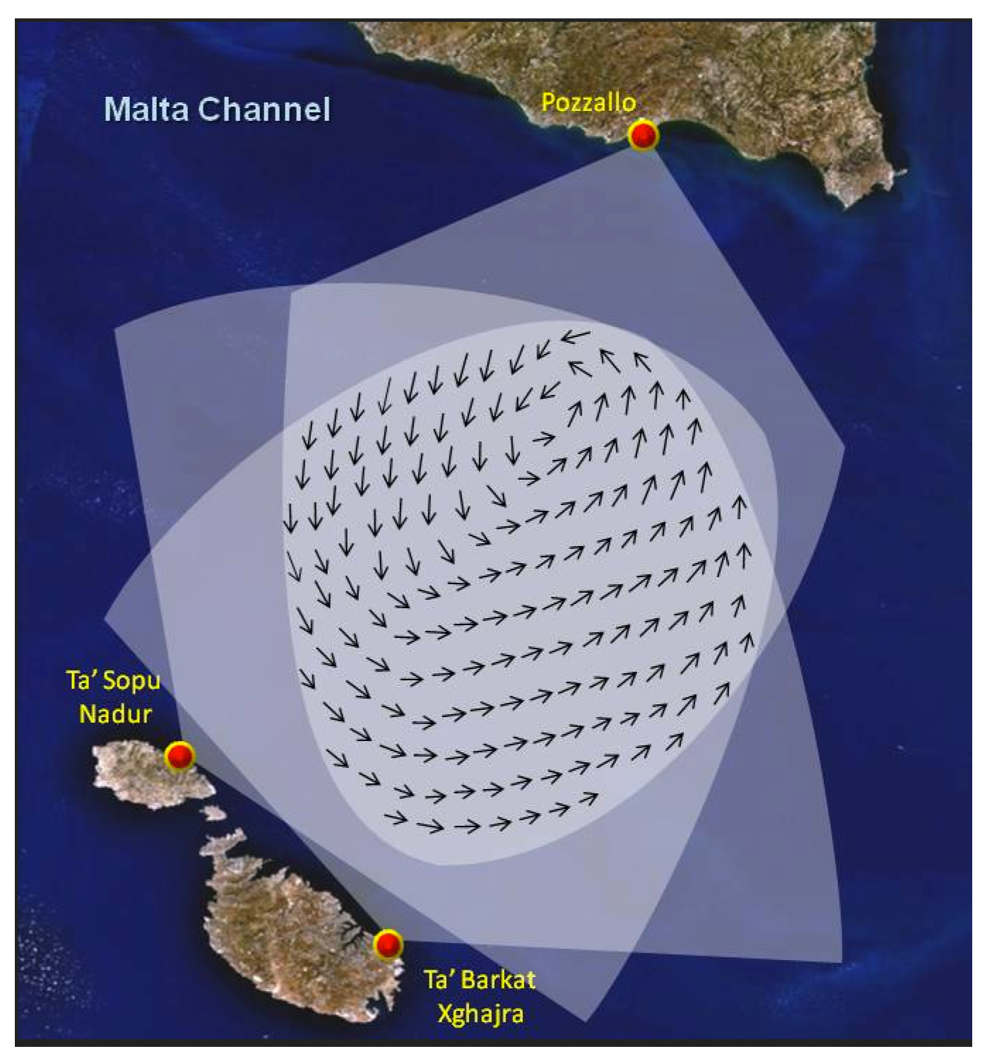
- The EMODNet (European Marine Observation and Data Network) surface currents in the Malta-Sicily channel given by the operational HF-RADAR observing system (CALYPSO Project, http://oceania.research.um.edu.mt/cms/calypsoweb/). These constitute hourly data with 1/37 horizontal resolution. The radar observing system is given by three antennas, two of which are placed on the Malta and Gozo Islands and a third one is located in the southern Sicily coast (Pozzallo) (see also Figure 12 [32]. The data are available from 2016 to present;
- The OGS (Istituto Nazionale di Oceanografia e di Geofisica Sperimentale) drifting buoys-derived sea surface currents and SST in the Mediterranean Basin. These lagrangian observations have six-hourly temporal resolution and the dataset coverage spans from 1986 to late 2016 (data doi=10.6092/7a8499bc-c5ee-472c-b8b5-03523d1e73e9);
- The CNR (Consiglio Nazionale delle Ricerche) Sea Forecast operational model for the computation of the three-dimensional surface currents, temperature, salinity, SSH, heat&water fluxes and wind stress in the Central Mediterranean (Tyrrhenian Sea and Sicily Channel). We were kindly provided with the monthly averaged data with nominal 1/48 horizontal resolution by the G3O-Operational Oceanography Group. More details available at http://www.seaforecast.cnr.it/forecast/index.php/en/forecast/sicily-strait-region/);
- The CMEMS Global Blended Mean Wind Fields. These are gap-free 6-hourly global data with 1/4 horizontal resolution computed at CERSAT/Ifremer. The data are available from January 2015 to present [33]. CMEMS data ID: WIND-GLO-WIND-L4-NRT-OBSERVATIONS-012-004;
- Two datasets of Sea Surface Salinity (SSS):
- The daily, 1/20 maps of L4 SSS obtained from the multifractal fusion applied to the L3 Soil Moisture and Ocean Salinity (SMOS) observations. The data are distributed by the Barcelona Expert Center (BEC) [34]. The data are available from 2011 to 2016;
- The 4-daily, 1/4 LOCEAN L3 SSS estimates derived from a combination of SMOS ascending and descending orbits measurements [35] and are available from 2010 to 2017.
In the list given above, the datasets labeled with 1 and 2 will be combined according to the method described in PIT09 to obtain the Optimal sea surface currents in the period 2012–2016. The Optimal currents will constitute a series of daily gap-free sea surface currents for the Mediterranean basin mapped onto a regular 1/24 grid (more details will be given in Section 3). On the other hand, the datasets labeled with numbers from 3 to 9 will be used for the quality assessment of the Optimal Currents, as we will show in Section 4.
3. Methods
3.1. Derivation of the Optimal Currents
Following PIT09 and RS18, we derive the surface circulation in the Mediterranean Sea combining the CMEMS geostrophic velocities (GV hereinafter) and the SST fields. The Optimal reconstruction is based on the inversion of the ocean heat conservation equation in the mixed layer. The equation, indicated below, is inverted for inferring information on the sea surface currents:
In Equation (1), (u,v) are respectively the zonal and meridional component of the ocean surface flow, (x,y) are the zonal and the meridional directions and F is the forcing term, containing the source and sink terms for the heat conservation equation. The resulting expressions for the optimally reconstructed velocity (u, v) are the following:
The Optimal currents are obtained adding the correction factors and to the background (“bck”) geostrophic velocities. In practice, Equation (2) is the formal expression of the synergy between the altimeter-derived SSH and the SST observations for the sea surface currents reconstruction. We provide a brief illustration of the terms appearing in the correction factors of Equation (2), referring the reader to PIT09 for more details. The correction velocities u and v have the following expressions:
In addition, is a function of the SST spatial derivatives, as expressed by Equation (4):
where A = SST, B = SST and (x,y) are the generic zonal and meridional coordinates. Moreover, in Equation (3) the functions f, g (expressed as functions of a generic variable ) and the coefficients p, q, and are given by the set of Equation (5):
where h is the error associated to the forcing term F; , are respectively the errors for the zonal and meridional background velocities, and E depends on the temporal derivatives of SST, i.e., E = SST-F.
The determination of the input parameters included in Equations (1)–(5) is illustrated in Section 3.2 and Section 3.3.
3.2. The Forcing Term F and the Computation of the Associated Error h
In RS18, the forcing term F was approximated as the satellite-derived, low-pass filtered SST temporal derivatives, only retaining spatial scales larger than 500 km. This choice is due to the following two facts:
- The lack of long and high-resolution time series of observed forcing terms estimates;
- The forcing term F of the SST heat conservation equation includes the vertical advection, the diffusion, the atmospheric heat fluxes and the entrainment velocity. At the first order, the main contributors to F are the atmospheric heat fluxes. In turn, the fluxes can be estimated as the large scales of the SST temporal derivatives, the smaller scales being related to the currents advection. This is also consistent with the analyses described in Rio et al. 2016 [24], who analyzed one year of MERCATOR model outputs at global scale (see, e.g., Figure 10 of Rio et al. 2016).
For the case of the Mediterranean basin, F was identified as the satellite SST temporal derivatives, SST, low-pass filtered at 400 km. This was achieved filtering the SST at several spatial scales and choosing the one that minimized the in-situ forcing estimates obtained with the OGS drifter-derived observations.
Using ≃ 30 years of drifting buoys-derived SST in the Mediterranean basin (data doi = 10.6092/7a8499bc-c5ee-472c-b8b5-03523d1e73e9), we computed an in-situ derived forcing term (F), whose formal expression is given by Equation (6).
where the subscripts “ins” and “t” respectively stand for in-situ measured and derivative with respect to time.
For every drogued buoy trajectory, we evaluated the in-situ daily dsst as
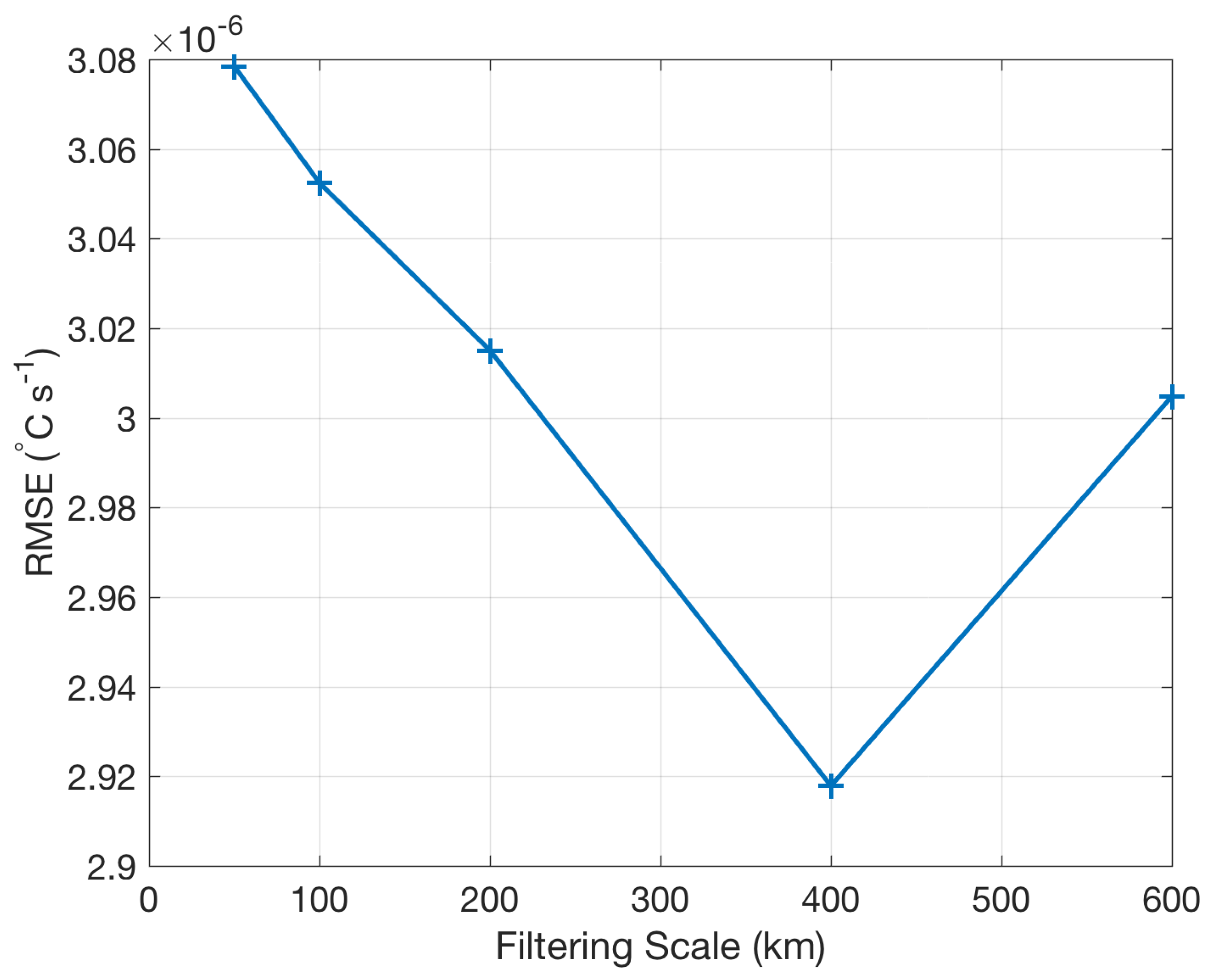
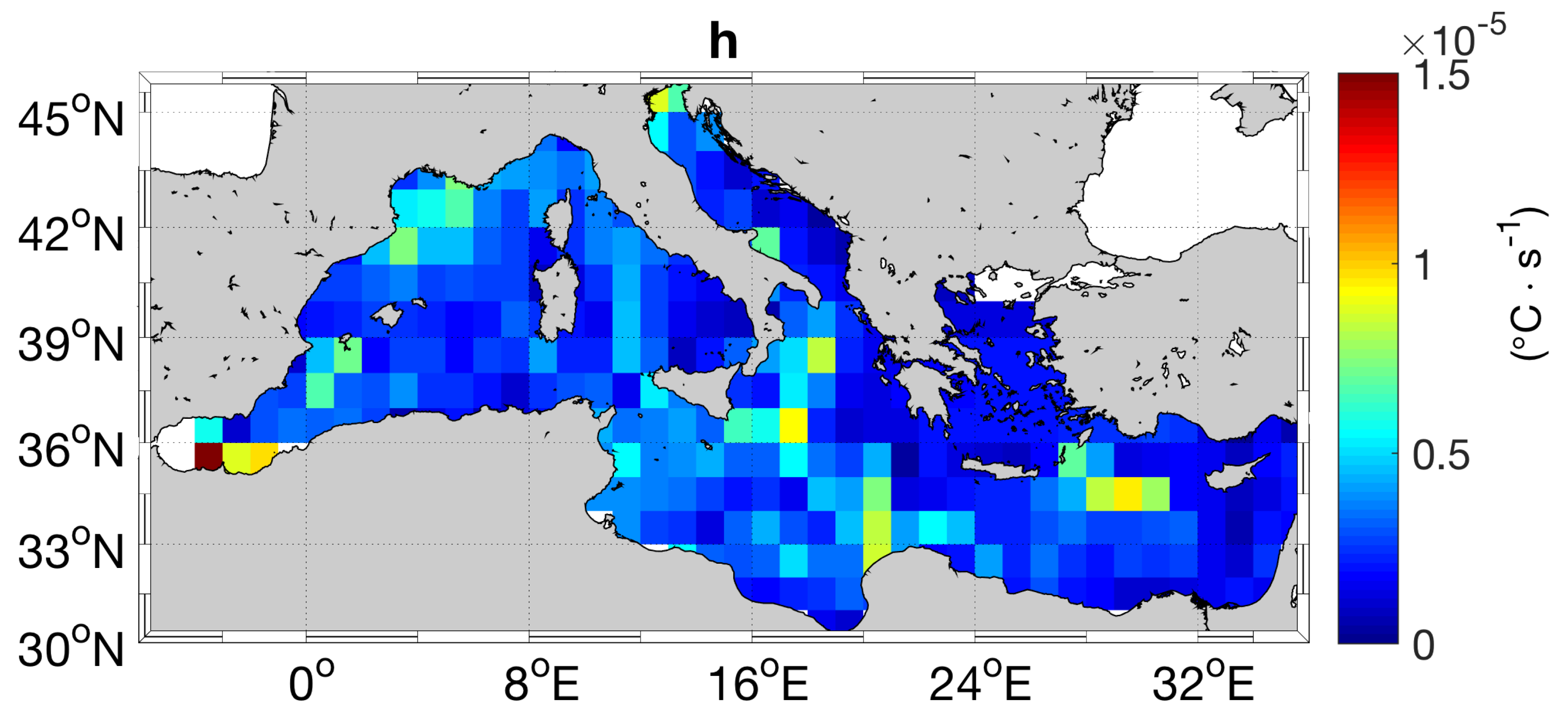
where dT = 1 day. Moreover, taking advantage of the 1986 to 2017 satellite-derived SST (dataset labeled with “2” in Section 2) we could compute the daily remotely sensed SST, including the filtered maps at scales ranging from 50 to 600 km. This operation enabled to derive the quantity L-SST, with L ∈ [50 km , 600 km]. Afterwards, each of the filtered L-SST was spatially and temporally colocated with respect to the drifters estimates, i.e., our benchmark. This allowed to generate two-dimensional maps of Root Mean Square Errors (RMSE) between the satellite and the in-situ-derived SST temporal derivatives. In the end, computing the mean, basin-scale RMSE between each of the L-SST and the , we found that for L = 400 km such RMSE reached a minimum (Figure 1) letting us identify it as the optimal filtering scale. In addition, we assumed that the RMSE error map between the 400 km-DSST and the SST is an estimate of the forcing term error h appearing in Equation (2). A map of h, binned in 1× 1 boxes, is given in Figure 2.
The order of magnitude of the RMSE is C·s over most of the Mediterranean Sea and its spatial variability is mostly correlated with the major dynamical features in the Mediterranean Sea (e.g., the Algerian current, the Liguro-Provenzal, the Atlantic Ionian Stream and Western Adriatic current) where the values can also exceed 1.5 C·s.
3.3. The Uncertainties on the Geostrophic Velocities (, )
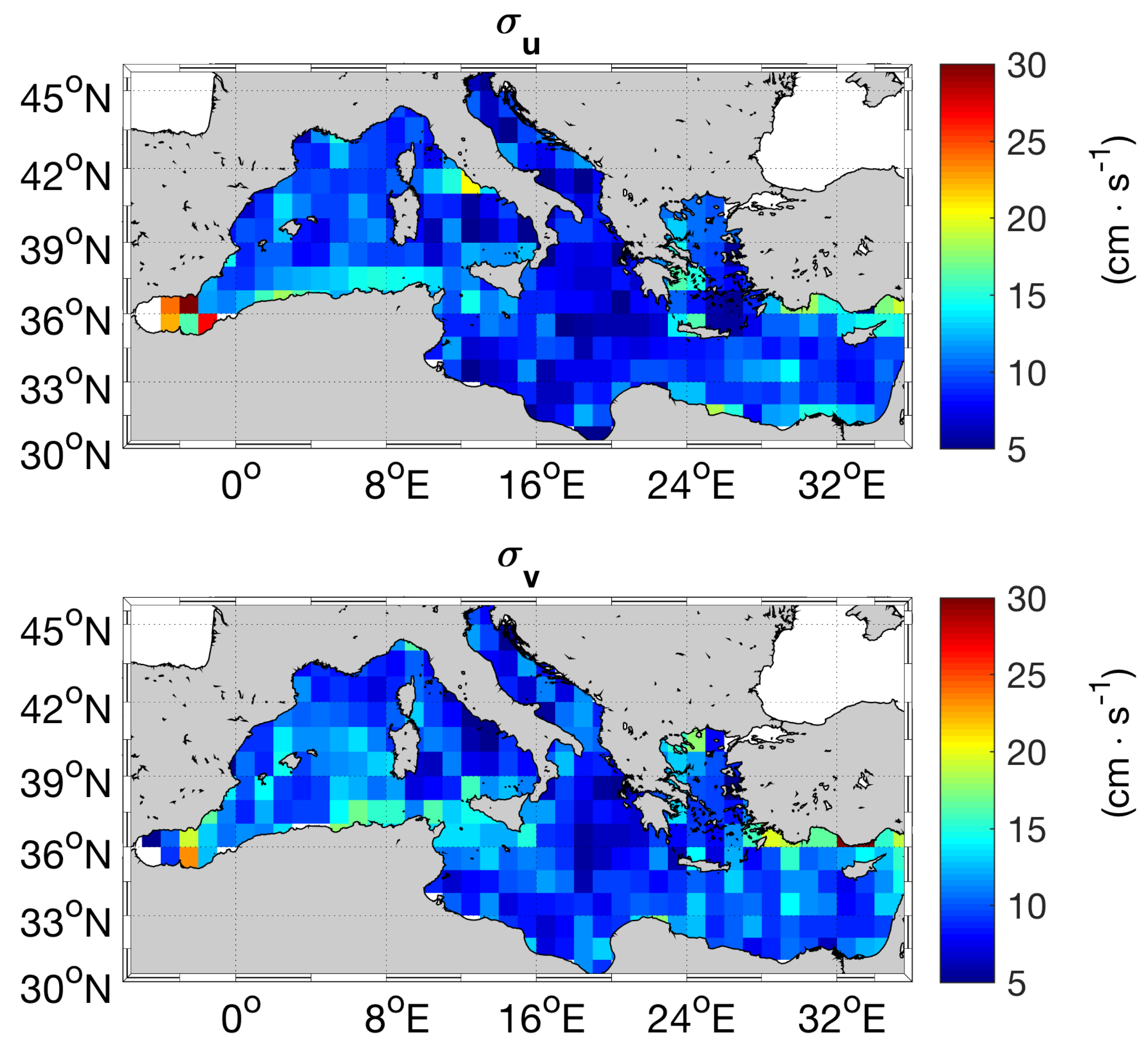
Another input parameter for the reconstruction method is the error on both the components of the surface geostrophic currents, previously defined as and for the zonal and meridional components of the current, respectively. This was estimated in a similar manner as for the forcing term, via comparison with the in-situ derived surface currents in the Mediterranean basin (data doi = 10.6092/7a8499bc-c5ee-472c-b8b5-03523d1e73e9). Using 24 years of altimeter-derived GV (introduced in Section 2) we could colocate the GV along the buoys trajectories and generate two-dimensional maps of the RMSE between the satellite and the in-situ measured currents. This was achieved selecting all the buoys evolving in presence of their drogue and binning the RMSE values in 1× 1 boxes, as illustrated in Figure 3.
The basin-scale mean error on the geostrophic velocities is of the order of 10 cm·s for both the components of the motion and it is slightly larger for the meridional component than for the zonal component of the motion (10.5 cm·s versus 9.6 cm·s, respectively). The maximum RMSE values can exceed 20 cm·s in correspondence of the Alboran gyres for both the surface flow components and their spatial variability is also correlated with the mean positions of the major currents in the basin. Indeed, the largest RMSE values (≥15 cm·s) are found in correspondence of the Algerian, Liguro-Provenzal, Libyo-Egyptian and Cilician currents as well as the Atlantic Ionian Stream [3].
4. Results
Relying on the CMEMS altimeter-derived GV, SST and on the error fields described in the previous section, we implemented the RS18 method to generate five years of Optimal currents in the Mediterranean Sea (from 2012 to 2016), a time window compatible with all the datasets used in the study. Such currents have spatial temporal resolution of and 1 day, respectively. In the following sections we discuss the Optimal currents performances with respect to the geostrophic estimates, mainly via validation against in-situ or model-derived data.
4.1. Case Study 1: Vortex Dynamics
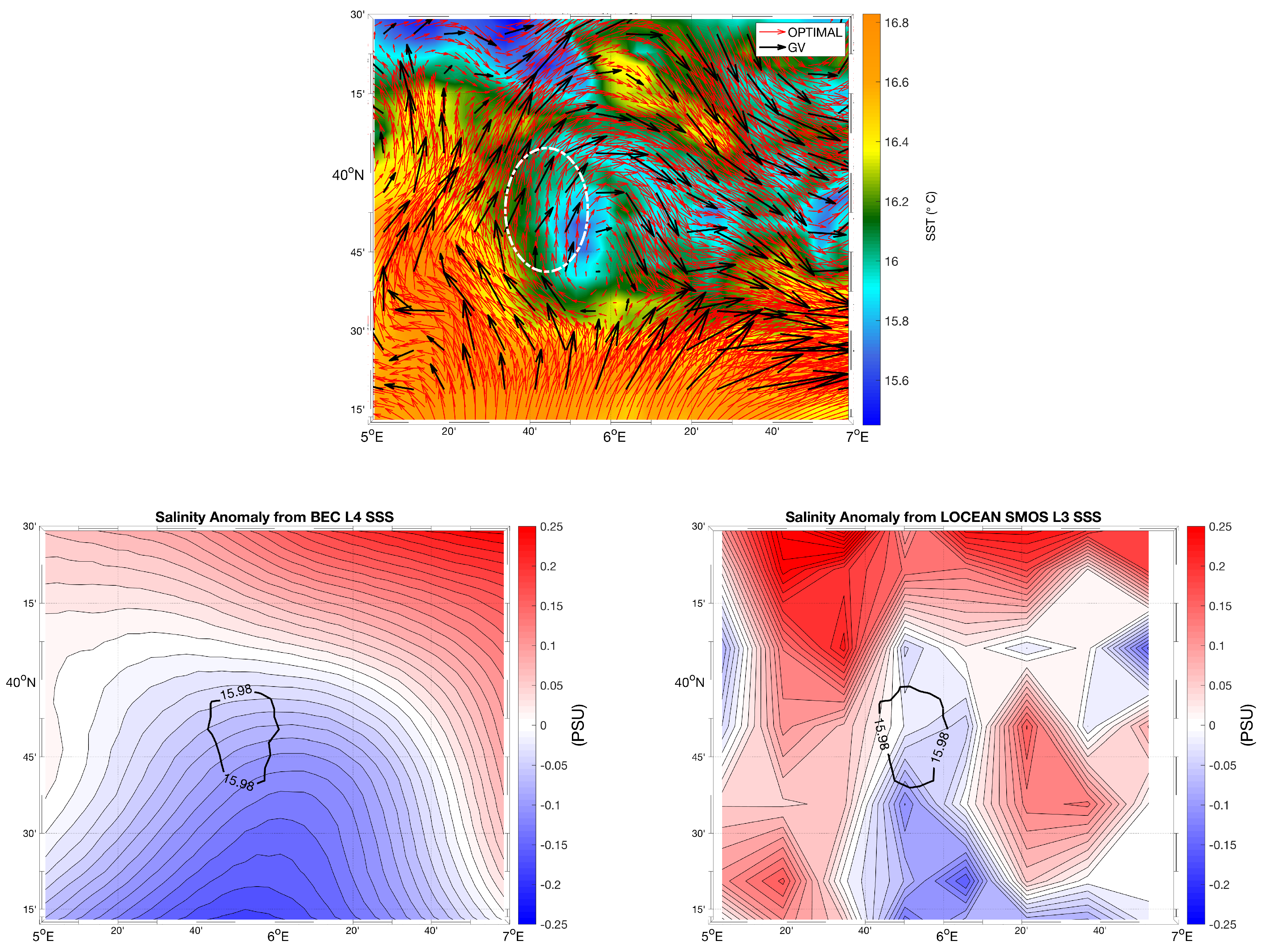
Here we give a first example of the Optimal Currents capabilities in presence of an oceanic vortex (generally referred to as eddy in the oceanographic community). An anticyclonic eddy located halfway between the Balearic Islands and Sardinia is detected on 25 April 2016 and is recognisable by a ring-shaped SST anomaly centered at approximately 3945N and 550E and is associated to a clockwise circulation (Figure 4).
Cold SST anomalies in presence of surface-intensified anticyclones have already been reported in literature [36,37]. In the Mediterranean sea, they can result from SSS compensation mechanisms, as also described in [16]. Using the Barcelona Expert Center SMOS L4 SSS for the Mediterranean Sea as well as the LOCEAN L3 SSS estimates (the latter being available on 26 April 2016), we found that the eddy lies in a negative salinity anomaly area. This is confirmed by the lower panels of Figure 4. Here, the eddy is highlighted by the 15.9 C closed contour and the SSS anomaly is evaluated as the SSS in the core of the eddy minus the SSS at the eddy periphery.
Thus, the salinity compensation mechanism is probably the cause of the observed oceanographic structure. However, the detailed investigation of the eddy formation and characteristics is outside the scope of this study. Here, we want to assess the capability of using the SST information to improve the altimeter-derived currents. In the western boundary of the vortex, the GV do not resolve such a dynamical feature, indicating a circulation which crosses the north western section of the eddy with a northeastward flow direction. This effect is a result of the mapping procedure statistics in order to obtain two dimensional maps from along-track altimeter data. On the other hand, if we consider the dynamical evolution of the SST, i.e., we account for the SST spatial-temporal gradients, the Optimal reconstruction method prescribes a correction factor that deviates the flow from the altimeter estimate, resulting in a more accurate description of the eddy circulation. This is particularly evident in the area highlighted by the white ellipse in the left panel of Figure 4.
This case study shows one of the main advantages of RS18, i.e., merging a background currents field with a higher resolution SST map. Other approaches, as SQG, rely on SST images to infer the surface flow. Nevertheless, when salinity anomalies contribute significantly to the sea surface density gradients, such approach may well lead to a current estimate which is in an opposite direction with respect to the actual one, as also found by Isern-Fontanet et al. 2016 [16]. Instead, using the RS18 method this ambiguity is overcome.
4.2. Case Study 2: Coastal Upwelling in the Sicily Channel
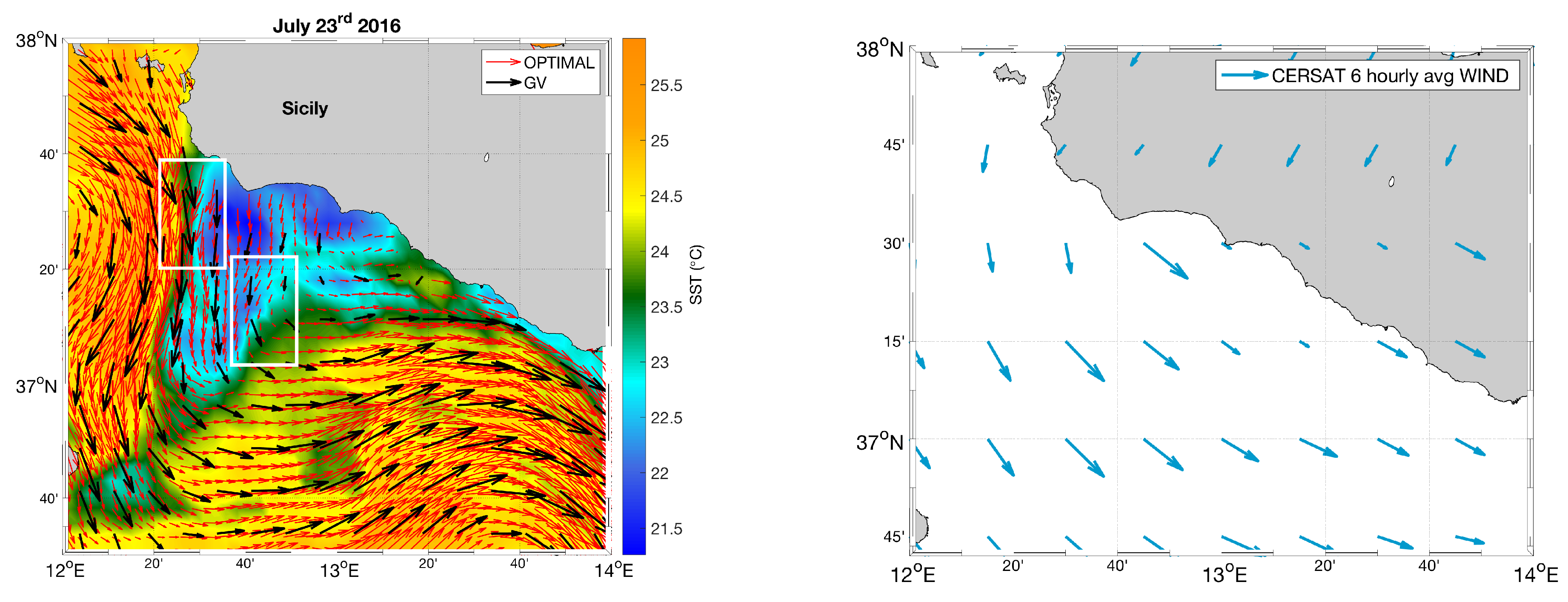
The Sicily Channel area, whose approximate coordinates are 11E to 13E and 36N to 38N constitutes an interesting testbed for the performances of the Optimal Currents. In this region, in proximity of the southern coast of Sicily, coastal upwelling is a very frequent phenomenon and is known to generate cold SST patches associated with an offshore directed current [38,39]. In particular Piccioni et al. 1988 [39], using a statistical approach, found that such events are mostly detectable during summer and that they mostly develop with a delay of three days with respect to the southeasterly wind input (i.e., with a non-zero alongshore component with respect to the southern coast of Sicily).
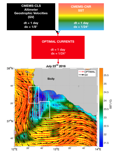
We show an example of coastal upwelling detected on 23 July 2016. The result of its dynamics is clearly visible from the SST spatial distribution and is consistent with the CERSAT/IFREMER averaged surface winds during the three previous days (20–22 July 2016) (Figure 5).
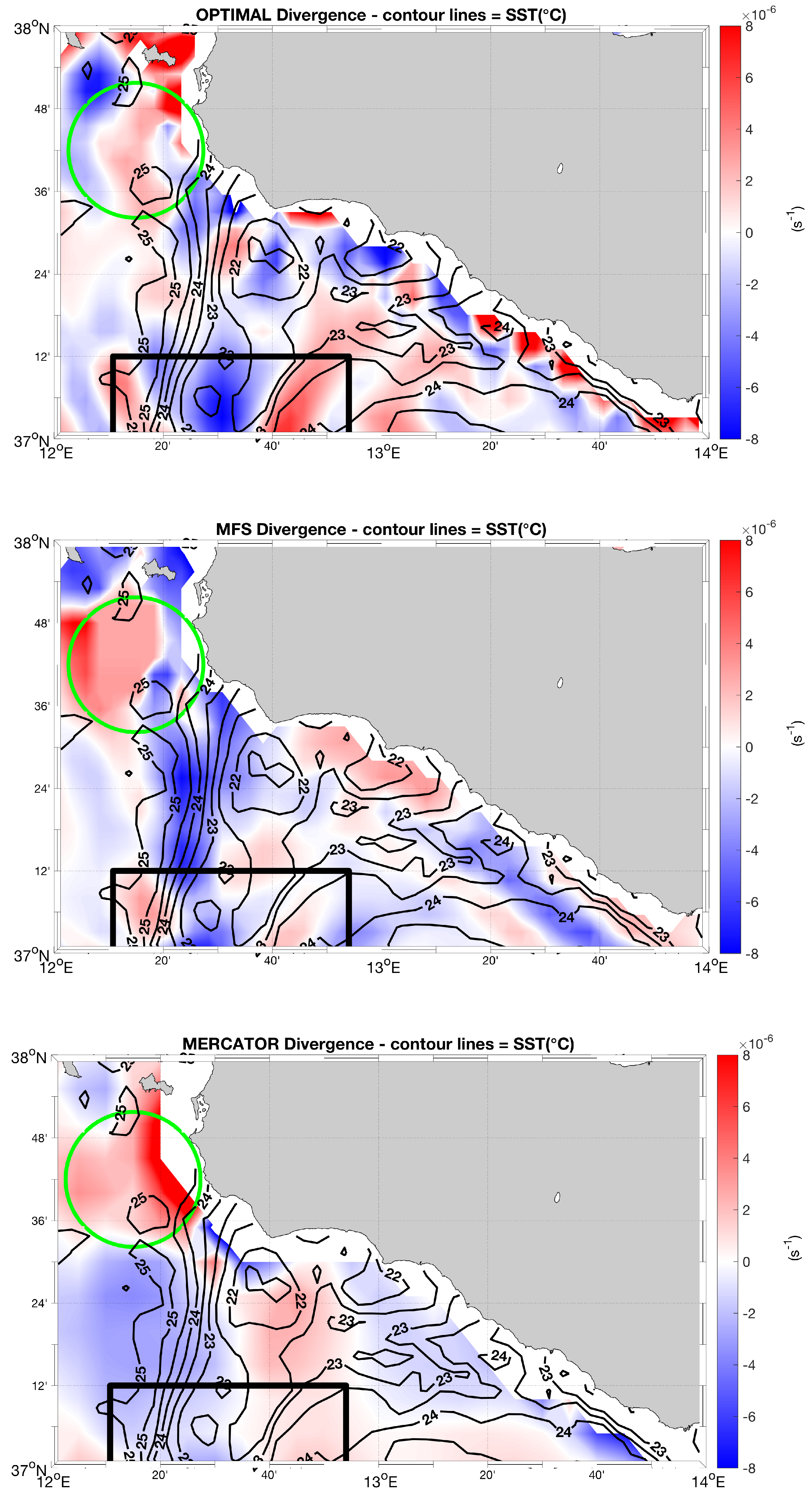
The SST anomaly between the interior of the upwelled waters and the surrounding areas exceeded 4 C and the shape of the patch (in agreement with the mechanism described in [39]) indicates an offshore current, perpendicular to the southern coast of Sicily (between 1220’E and 13E). The offshore circulation was not entirely captured by the GV (Figure 5). Indeed, at the positions 1240E–3730N and 1220E–3715N, highlighted by the white boxes, the GV exhibit a cross thermal gradient component which is not consistent with the wind-driven circulation. A cross-thermal gradient geostrophic circulation is also found in correspondence of the lower tip of the cold SST patch. This effect is reduced when the Optimal reconstruction is implemented. The qualitative validation between the GV and the Optimal currents patterns allows to conclude that, enriching the GV with the information contained in the spatial and temporal variability of SST, it is possible to retrieve the ageostrophic circulation (as it is the case for the wind-driven upwelling dynamics) starting from the geostrophic, altimeter-derived currents. In order to further confirm this, we computed the divergence of the surface currents field. The divergence is defined as (with u and v the generic zonal and meridional components of the motion, respectively). When applied to a geostrophic field, the divergence operator yields zero in the whole surface currents domain, while it can be (10 s) for a total surface current field, i.e., considering both the geostrophic and the ageostrophic components of the motion [40]. Indeed, choosing the same region of Figure 5, we compared the divergences obtained using the Optimal currents, the model-derived surface currents of the MFS operational model and the MERCATOR global operational model (Figure 6). In addition, a comparative analysis with the monthly outputs of the CNR-Sea Forecast operational model will be given. Such divergences were all computed using a 9-point stencil width technique, as in [41].
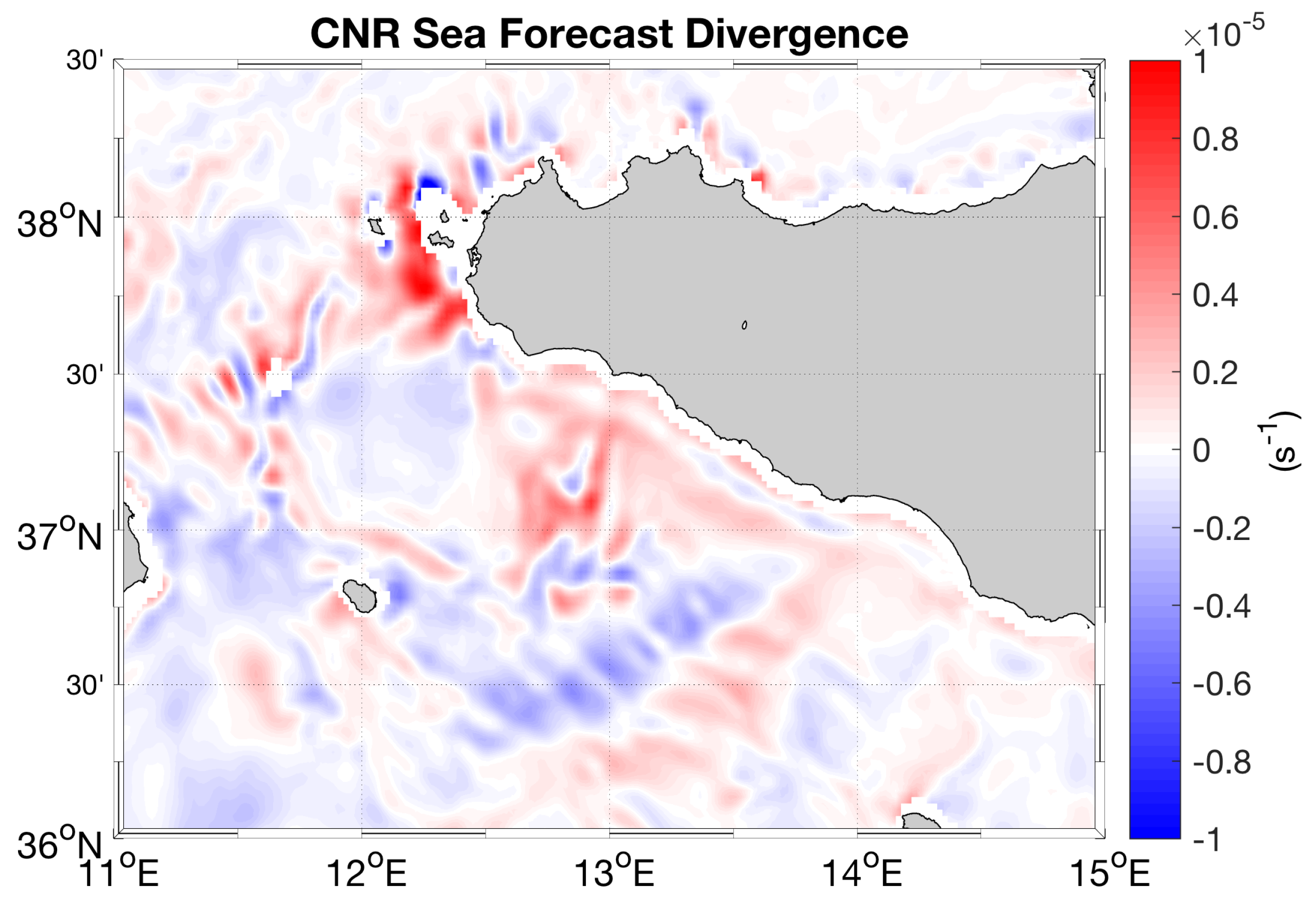
The GV, though not exhibiting divergence values strictly equal to zero (mostly due to the numerical scheme of the computation), were mostly (10 s) everywhere in the analyzed area, (as well as in the rest of the Mediterranean Basin (not shown). Thus, we assumed this order of magnitude to be the lower limit for the surface currents field divergence, that can be referred to as geostrophy. On the other hand, the upper limit for the divergence values is identified with the results given by the MFS operational model. In this case, the divergence could reach the value of × 10s (bottom panel of Figure 6). Quite interestingly, the Optimal currents exhibit divergence values at least two orders of magnitude larger than the GV, up to s, hence comparable with the ones of a total surface current. The current field of the MERCATOR operational model also exhibits values ( s), though its maxima only reached the 70% of the values observed in both the Optimal and the MFS-model case. Moreover, using the monthly averages of the submesoscale-permitting (resolution ≃ 2 km) operational model for the Sicily Channel and Tyrrhenian Sea (dataset labeled with “7” in Section 2), we had further confirmations that the expected value of the surface currents divergence during July 2016 must be ( s), as also shown in Figure 7.
In addition, if we compare the spatial distribution of the divergences (DIV hereinafter) of the Optimal, MFS and MERCATOR surface currents (for 23 July 2016), the following similarities can be found:
- The presence of an overall flow divergence area (DIV > 0) off the western cape of Sicily, around the Egadi Islands, highlighted in light green in Figure 6, with some convergence areas intrusions found in both the MFS and the Optimal Currents estimates;
- The alternating flow convergence (DIV < 0) and divergence (DIV > 0) patterns inside the cold SST filament extending almost vertically from 3736N–1220E to 3700N–1220E. Such adjacent patterns are mostly found around 3706N and are highlighted in black in Figure 6. They are common to all the current fields, though looking smoother in the MERCATOR estimates.
The most interesting result of this comparison is that the combination of the geostrophic current and the SST data is a promising technique for the retrieval of the total surface current field from an initial geostrophic estimate, i.e., the one provided by satellite altimetry. Indeed, the Optimal current divergence is of the same order of magnitude predicted by high-resolution numerical models and observations, also sharing common features in the spatial patterns given by the MERCATOR and MFS-model estimates (though in the numerical model outputs the structures are slightly smoothed compared to the Optimal case).
In the following sections we will describe the quantitative validation of the Optimal currents via two approaches: a first one in which the comparison will be performed with respect to the in-situ drifting buoys measurements in the Mediterranean Sea and a second in which the Optimal currents will be compared to the estimate of the High-Frequency Radar (HFR hereinafter) surface currents in the Malta–Sicily channel.
4.3. Validation with the In-Situ Measured Currents
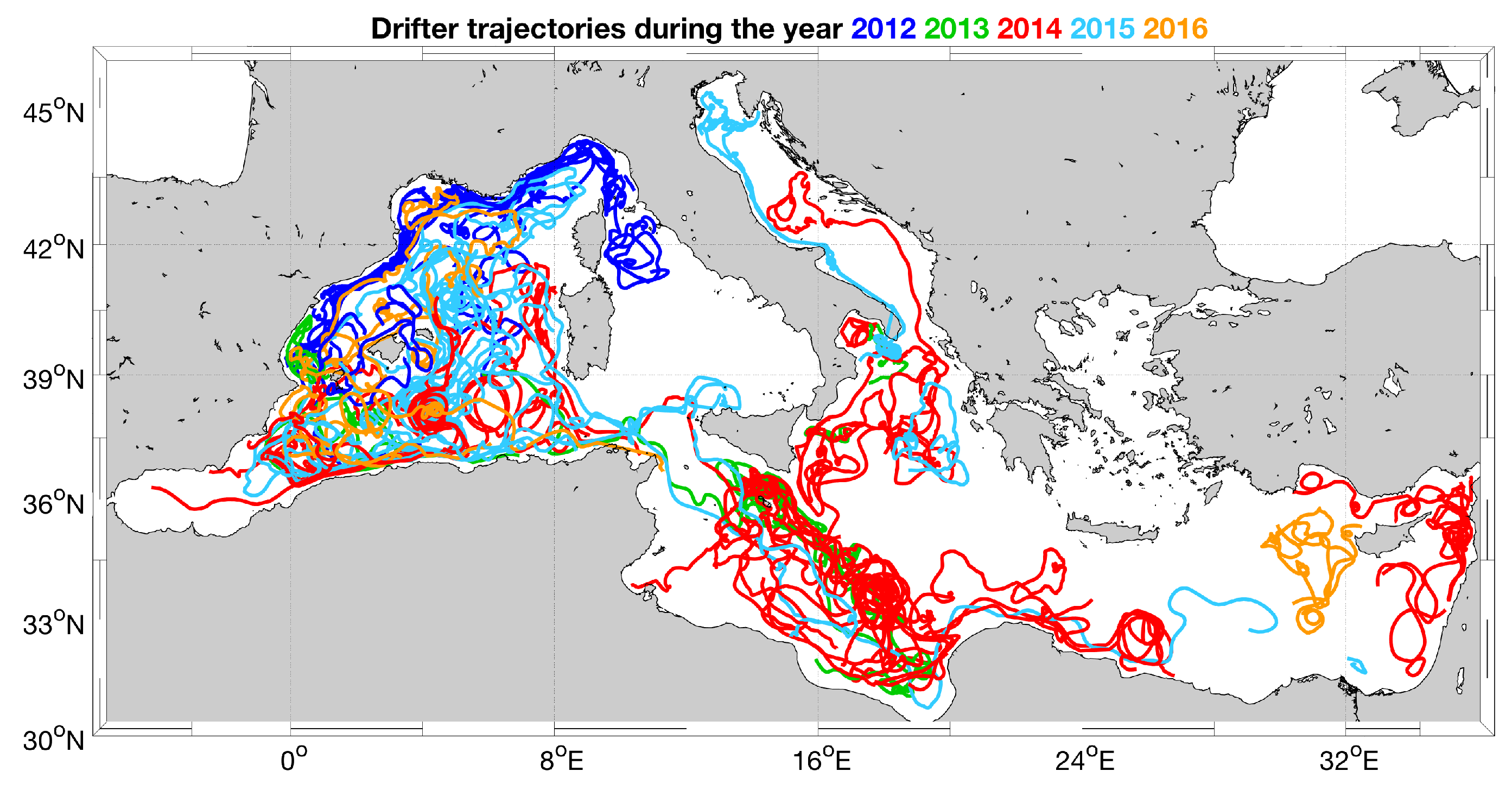
In the period 2012 to 2016, the in-situ sea surface currents have been deduced from the trajectories of 104 15m-drogued drifting buoys at the positions indicated in Figure 8 (data doi = 10.6092/7a8499bc-c5ee-472c-b8b5-03523d1e73e9, [42]).
The buoys have been mostly occupying the Western, the Central Mediterranean Sea, the Adriatic Sea and the area around the Island of Cyprus (eastern Mediterranean), measuring the sea surface currents with 6-hourly temporal resolution. Selecting the totality of the buoys trajectories, we compared the performances of the GV and the Optimal currents against the in-situ-derived measurements. This was achieved creating two match-up databases for the GV and the Optimal currents, which are both gridded fields. The match-up database was generated using cubic interpolation for the spatial colocalization of the gridded currents over the buoys positions while a linear interpolation was used to create the 6-hourly GV and Optimal currents (which are originally daily data) and finally perform the colocalization in time.
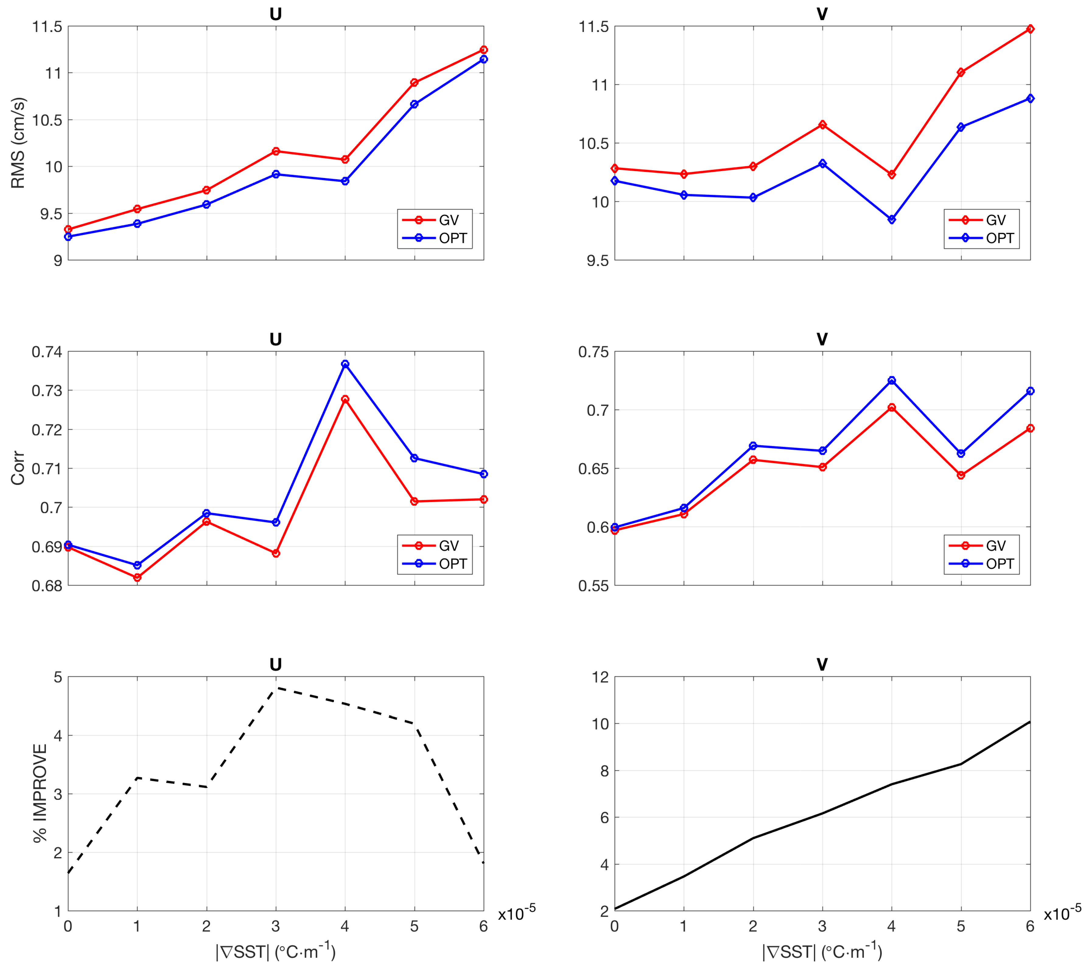
Similarly to RS18, the validation is based on the computation of the RMSE, correlation coefficients (CC) and biases between the GV, the Optimal currents and the drifter-derived currents, the latter being our benchmark. The computation of the biases did not evidence significant differences between the GV and the Optimal currents. For both datasets, the basin scale bias of the zonal and meridional component of the motion is around −0.3 cm/s and 0.4 cm/s, respectively. Concerning the RMS, the Optimal currents always exhibited lower values than the ones obtained with the GV, with larger RMSE reduction for the meridional component of the motion. Moreover, we found that the difference between the GV and the Optimal currents RMSE increases with the increasing magnitude of the SST spatial gradients (A,B in Equation (4)), indicating that our reconstruction method gives the best performances in large SST gradient areas. This was found selecting all the GV and Optimal current values laying in areas of progressively increasing |∇SST|, with |∇SST|= comprised between 0.1 and 6C·m (such interval represents more than 90% of the |∇SST| values in the basin). Based on the RMSE computation, we also defined a parameter to estimate the percentage of improvement of our reconstruction method with respect to the GV estimates. The parameter is defined as follows:
where U,V respectively indicate the zonal and the meridional component of the sea surface currents.
In general, our reconstruction is more satisfying for the meridional component of the motion and, at the basin scale, yields improvements that can exceed 10% (while they are only about 5% for the zonal component of the motion). Such improvements increase almost monotonically with the magnitude of the |∇SST| except for the zonal currents, where a linear increasing trend is only observed until 5 C·m. In a similar fashion, the Optimal currents show correlations with the in-situ measured currents generally higher than the GV, with a correlation improvement which is larger for increasing |∇SST| values. Such results, schematically summarized in Figure 9, indicate that the Optimal currents better represent the sea surface currents variability observed via the in-situ measurements, confirming the potentiality of bringing the spatio-temporal variability of the SST remote observations inside the large-scale geostrophic currents.
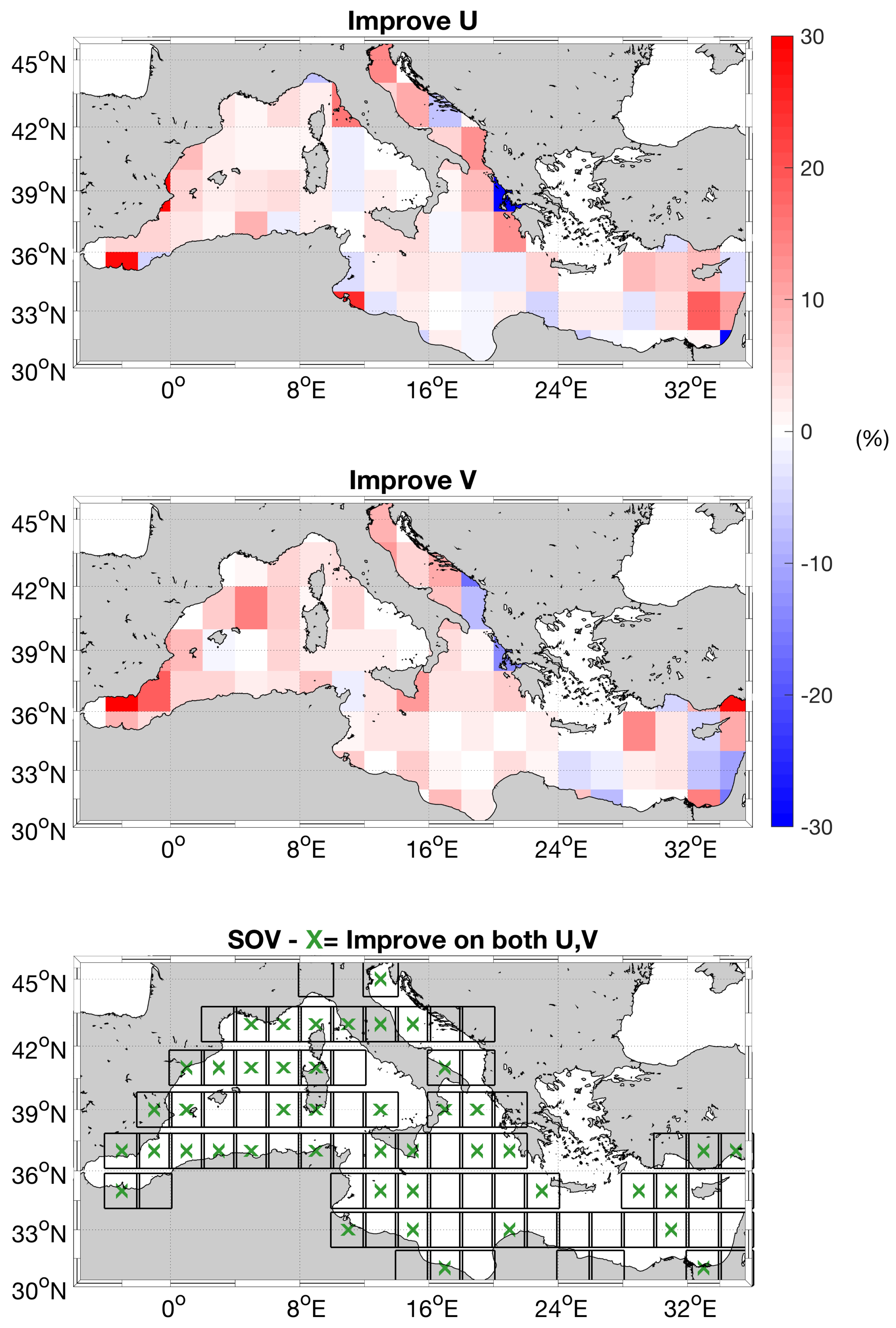
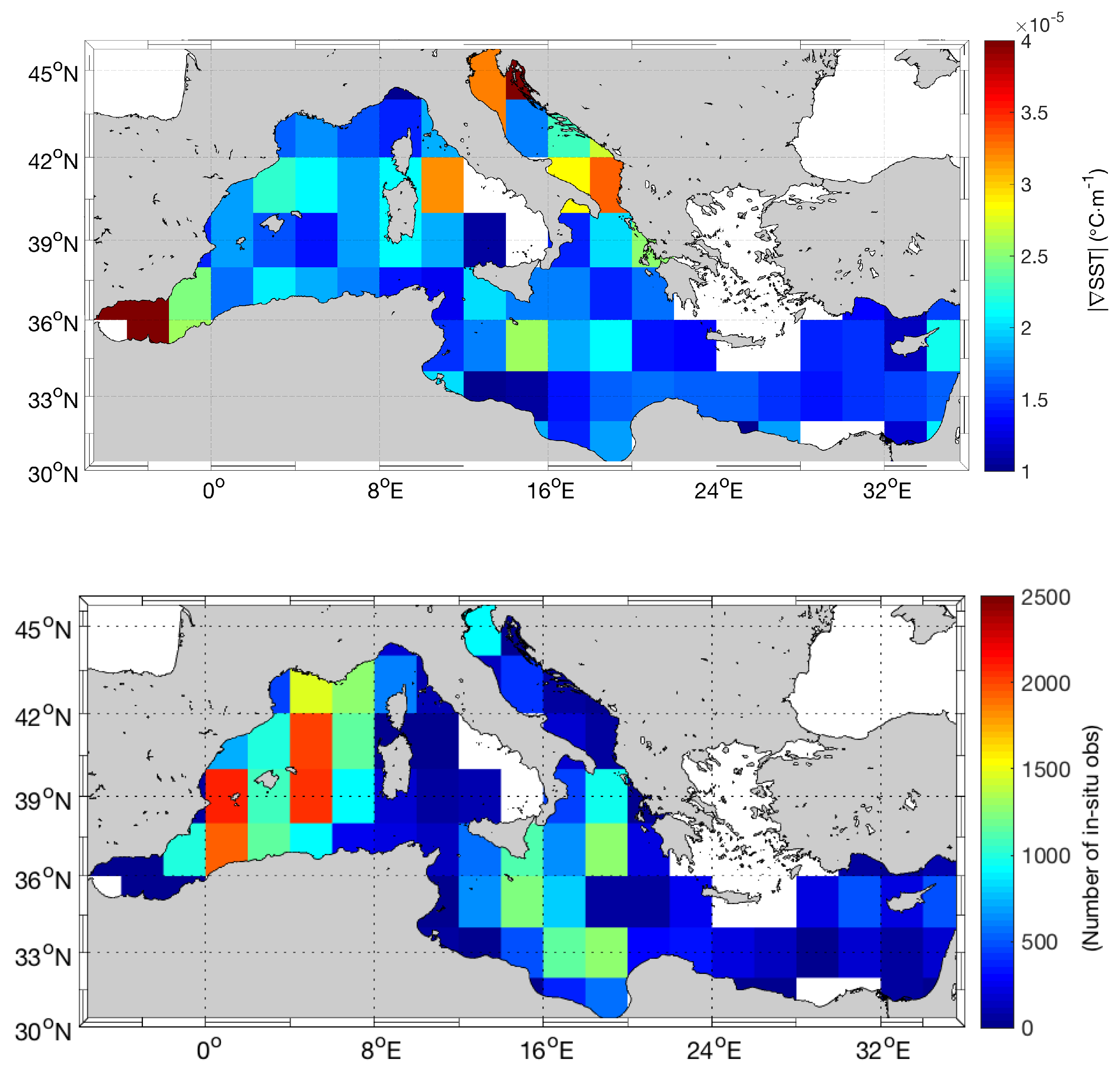
During 2012–2016 we also investigated the local variability of the Optimal reconstruction method. This has been done binning the values obtained using Equation (7) in 2 2 boxes (Figure 10 upper panels). The available drifter-derived currents allowed to perform the analysis in the sites of validation (SOV) indicated by the black squares in Figure 10 (bottom panel). In general, the best performances are found in the Central and Western Mediterranean, where local improvements can also reach 30%. The results of the validation, both at the basin scale and in terms of local variability, are in agreement with the results found at global scale by RS18. Also, we found that in the Western Mediterranean, the summertime reconstruction can lead to improvements exceeding 40%, which was not found during winter (not shown). Considering our investigation area, the zonal component of the surface currents is improved over 60% of the domain, while this percentage raises up to 70% for the meridional component of the motion. Combining these results, we could also indicate all the SOV where the method can improve both of the surface flow components, schematically given in the bottom panel of Figure 10. As expected, such SOV are mostly located in the Western Mediterranean. Unfortunately, some of the sites of the Optimal currents validation, though never exceeding the 40% of the analyzed domain, indicate that the method can also degrade the quality of the surface currents, when compared to the geostrophic estimates. These sites are mostly located in the eastern section of the Mediterranean basin. Quite interestingly, they are characterized by two properties: either they lay in areas of low |∇SST| (≃0.1 C ·m), which is not the ideal condition for the method applicability, or their statistical properties are computed based on a poor number of observations, affecting their statistical significance. This can be checked comparing the maps of |∇SST| and numbers of available in-situ observations binned in 1 1 boxes in Figure 11. In a future study we plan to compute such statistics on a longer time series of optimal currents (≃20 years) and check the effects on the local variability of the optimal reconstruction method performances.
Nevertheless, it is worth noticing that the validation against the in-situ observations confirmed the validity of the case study analyzed in Section 4.2. Indeed, in the coastal area of the Sicily Channel (close to the southern coast of Sicily), during the period 2012–2016, our surface-currents reconstruction method yielded positive improvements for both the components of the motion. Hence, we wanted to further investigate the quality of the Optimal currents via a comparison with the HFR-derived surface currents in the Malta–Sicily Channel. The results are presented in Section 4.4.
4.4. Comparative Analysis: Optimal Currents Validation in the Malta–Sicily Channel
In this section we present an additional quality assessment for the Optimal currents via comparison with the daily surface currents derived from the Calypso High Frequency Radar platform in the Malta–Sicily Channel (during the year 2016), our benchmark. The coverage of the Calypso platform, schematically shown in Figure 12, extends from 35.7N to 36.8N and from 13.7E to 15.2E. As stated in Section 2, such platform provides hourly observations at 1/37 horizontal resolution, hence, our validation was realized creating daily maps of HFR currents. For each day, we computed bias and root mean square errors of the differences between the GV, the Optimal, the MERCATOR, the MFS-derived currents and the HFR estimates. Unfortunately, no comparison with the drifting buoys-derived currents was performed as, during the year 2016, the buoys have been circulating in the westernmost and easternmost sections of the Mediterranean basin only (Figure 10).
Unlike the case of the drifting buoys, the comparison with the High-Frequency Radar (HFR) currents involves two-dimensional gridded data. In order to carry out the comparison, all the analyzed daily currents were remapped over the HFR grid via bi-cubic interpolation. The mean results of the comparative study are summarized in Table 1 and Table 2.
Focusing on both the Optimal and the GV, using the HFR estimates as benchmark, the current retrieval is more satisfying for the meridional component of the motion, exhibiting lower RMSE and BIAS (respectively ≃9.00 and ≃1 cm·s) compared to the zonal one, where RMSE and BIAS are respectively ≃10.00 and ≃4 to 5 cm·s. Moreover, if we observe the behaviour of the Optimal currents with respect to the other datasets, we find that the RS18 method brings larger improvements on the retrieval of the zonal component of the motion. Indeed, for such component the Optimal currents have the lowest RMSE of all, 9.72 cm·s (the MFS model yielding the larger value, 12.70 cm·s) and a lower BIAS (4.04 cm·s) than the GV and the MERCATOR estimates. The only exception is given by the BIAS of the MFS model, whose value is ≃3 cm·s.
For the meridional component of the motion, the Optimal currents have RMSE and BIAS in line with the GV and always lower than the numerical model estimates. These results may look surprising. Indeed, at the basin scale the RS18 method brought the largest improvements for the meridional component of the motion. Nevertheless, here we are restricting our analysis to a much smaller coastal area in which our reference, the HFR currents, are known to be more accurate in retrieving the zonal component of the motion [43], probably affecting the statistics on the meridional flow.
Considering these results, we can conclude that the Optimal currents perform globally better than altimeter-derived estimates or model outputs.
5. Discussion and Conclusions
During the last decades, both physical and operational oceanography have been demanding high spatial and temporal resolution observations. Such observations are useful for the validation, optimization and run of the main operational models, especially when data assimilation is required. In the specific case of the sea surface currents retrieval, the high-resolution and repetitive observations are also necessary for several human activities in the marine context (navigation, safety and rescue activities) and for the environmental safeguard (illegal oil spills and pollutants monitoring).
The objective of our study was to improve the spatial and temporal resolution of the remotely sensed, altimeter-derived surface currents in the Mediterranean Sea. Based on the RS18 method, we could successfully introduce the information contained in a high-resolution satellite-derived SST (t = 1 day and x = ) inside the larger scale altimeter geostrophic currents. The RS18 method has the main advantage to optimize the use of SST to derive information on the surface currents field. This is achieved accounting for the source and sink terms in the SST evolution equation, unlike in maximum cross correlation techniques where only advection and diffusion can be considered. An additional advantage of the RS18 method is the possibility to rely on a background surface currents estimate, i.e., the altimeter measurements. This enables to derive the surface circulation even in areas of low tracer gradients or when the tracer alone is not a direct proxy of the ocean surface dynamics [16]. We applied the RS18 reconstruction method to the CMEMS datasets of geostrophic surface currents and sea surface temperature satellite data for the Mediterranean area. This enabled to estimate an Optimized velocity during five years.
The highlights of our study are listed here:
- During the period 2012–2016, we computed daily gap-free maps of Optimal currents. Using the OGS in-situ measured surface currents as a benchmark, we compared the performances of the Optimal currents and the altimeter-derived estimates. We found that the Optimal reconstruction method yields the largest improvements (locally up to 30%) in the western section of the Mediterranean basin and for the meridional component of the motion. Such improvements generally increase with the increasing SST spatial gradients and proved to be slightly higher during summertime. This is mostly due to the larger spatial SST gradients that can occur during summer, especially in areas of upwelling. This effect is particularly enhanced in the Western Mediterranean and in the Sicily Channel area, where you have very active upwelling regions (not shown);
- The Optimal reconstruction method is able to retrieve both the small scale geostrophic and ageostrophic circulation, obtaining a surface field characterized by a non-zero divergence. This was shown for the Sicily Channel. In this area, during summertime, it is frequent to observe patterns of ageostrophic circulation. Indeed, computing the Optimal currents during a coastal upwelling event (on 23 July 2016), we found that the surface divergence of the Optimal currents is comparable with the predictions of the CMEMS operational models, providing an estimate of the total (i.e., with non-zero divergence) surface-current field. The values of the Optimal currents divergence also proved to be in line with the monthly values predicted by the submesoscale-permitting CNR-Sea Forecast operational model for the Sicily Channel;
- The Optimal reconstruction, unlike the SQG method, allowed to overcome the ambiguity in retrieving the surface circulation when SST is not a direct proxy of the surface circulation. In this study, this was proved for a specific eddy dynamics case study in the Western Mediterranean area.
- In the Malta-Sicily channel, using the HFR surface currents as our benchmark, the Optimal currents improved the mean RMSE and BIAS compared to the numerical model outputs and to the satellite-derived currents (except for the bias in the retrieval of the zonal flow, where the MFS model exhibited the best performance).
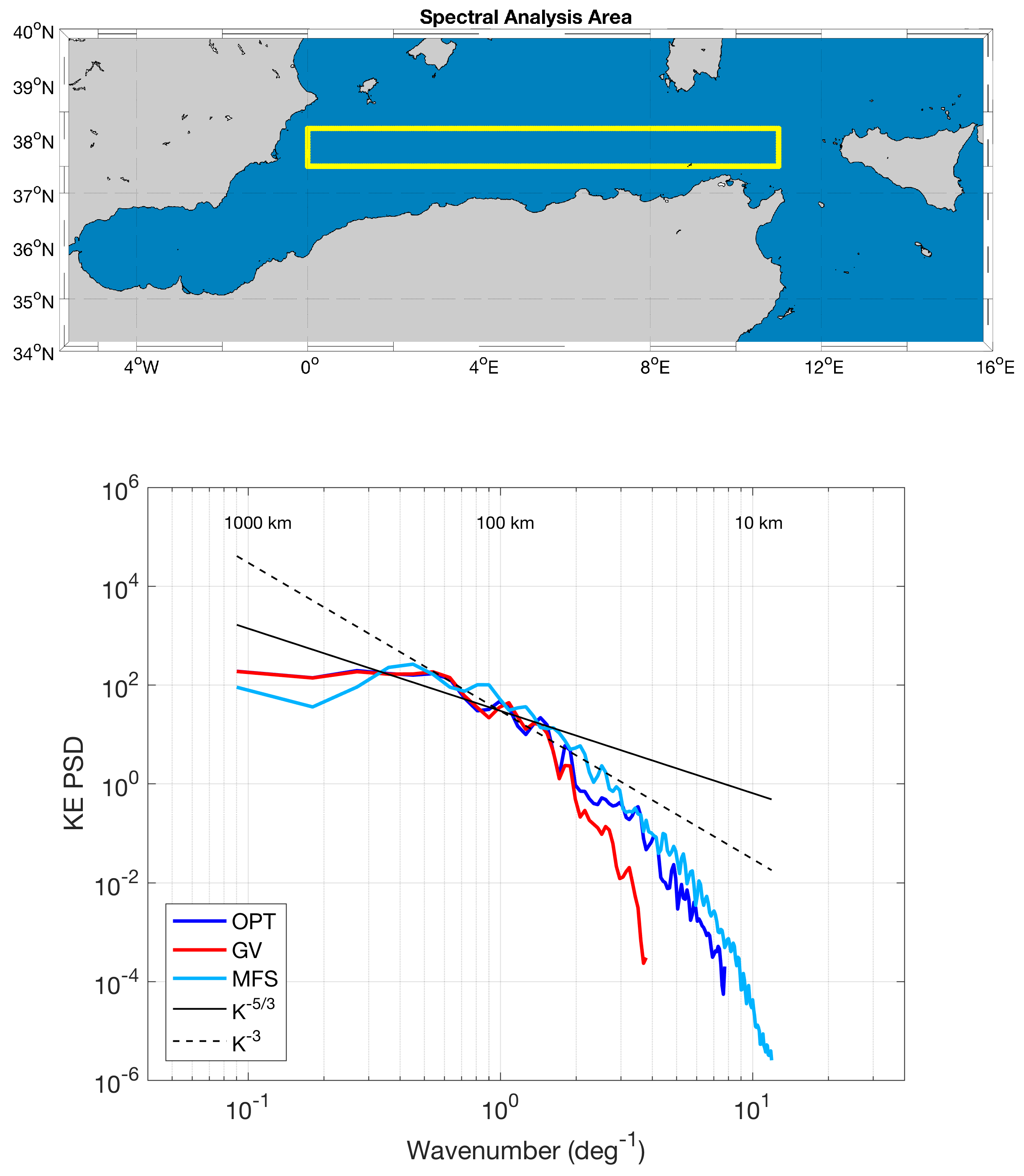
The main results listed here express the capability of the RS18 method to increase the spatio-temporal variability of the altimeter-derived currents even in the Mediterranean Area. Provided the existence of non-zero sea surface temperature spatial gradients, the variability of the high-resolution SST data can be successfully introduced inside the large-scale geostrophic currents estimates. The increase in the spatio-temporal variability explains the satisfying comparison of the Optimal currents with both the in-situ measured currents and the HFR estimates. Moreover, this was confirmed by the spectral analysis shown in Figure 13. In particular, we computed the mean spatial Kinetic Energy (KE) spectrum of the Optimal, MFS and altimeter-derived surface currents (GV) as a function of the spatial wavenumber (here given as the inverse of the wavelenght.) This was done in a land-free and dynamically active area of the Western Mediterranean (37.5N to 38.0N and from 0E to 11E), delimited by the yellow box in Figure 13. Moreover, we performed this analysis done during summertime (on 23 July 2016) i.e., choosing all the favourable conditions for the Optimal reconstruction method. Looking at the behaviour of the KE power spectral density, we can see that the Optimal currents and GV power spectra are superimposed until a scale of 100 km. Afterwards the GV begin loosing energy and their spectrum falls abruptly. Such a result was expected and is intrinsic with the geostrophic large-scale estimate of the surface currents, whose spectral content is mostly in the mesoscale range. On the other hand, for scales smaller than 100 km, the Optimal Currents spectrum contains more energy than the GV one and maintains the same decreasing trend until a scale of 30 km, confirming that the resolution of the Optimal currents is actually increased with respect to altimetry (notice that in the figure we discarded the areas in which the spectra exhibit a noisy behaviour). Moreover, the Optimal Currents spectrum is in agreement with the predictions of the MFS model, that, based on a fully three-dimensional primitive equations framework, simulates the evolution of the total currents field. Quite interestingly, Figure 13 also confirms that the Optimal and MFS spectra are closer to the predictions of the two dimensional turbulence energy cascade, K and K [44]. Though the K slope is not fully recovered at small scales, the Optimal Currents spectral separation from the K line is reduced compared to the altimeter estimates.
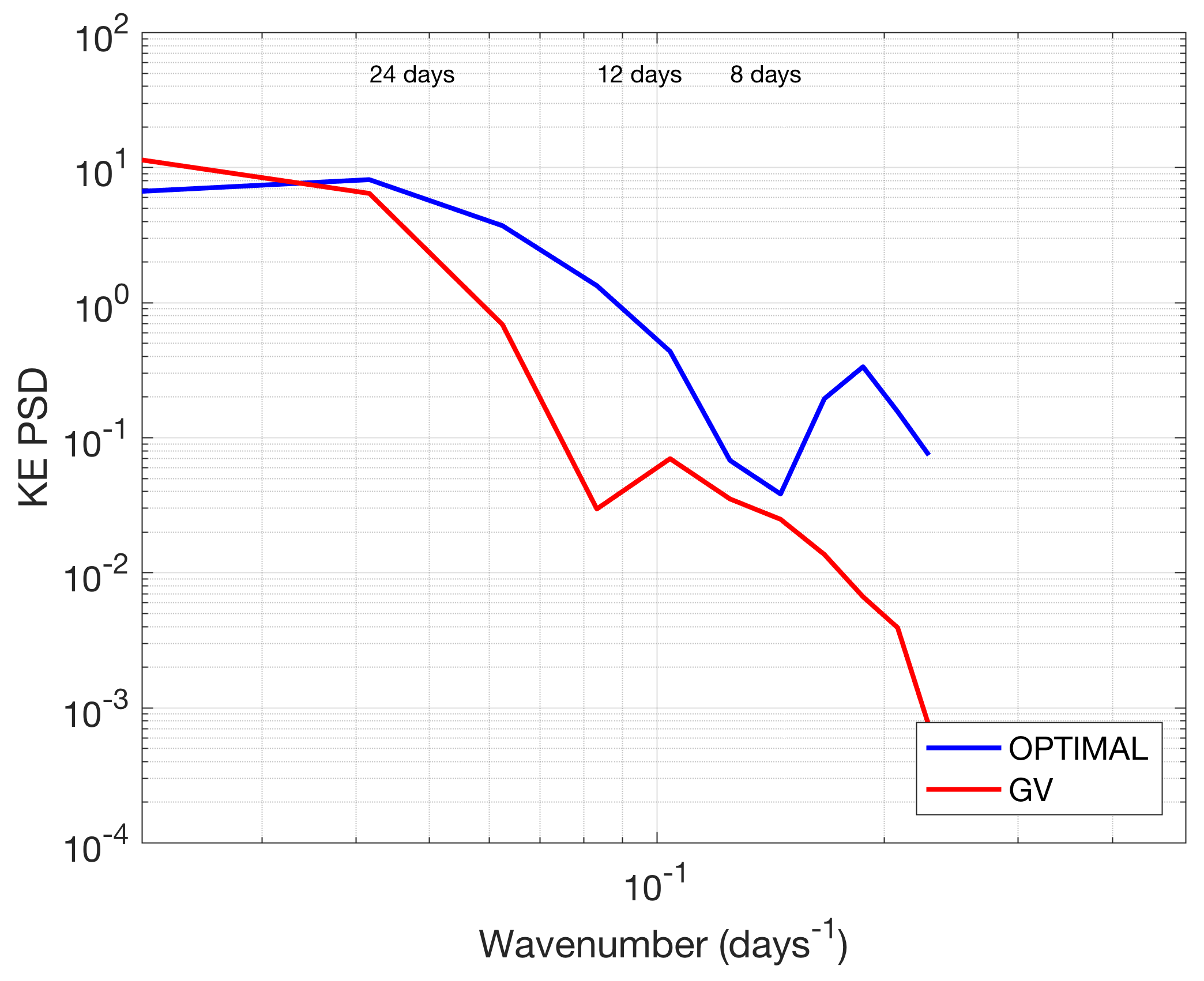
In the end, we computed the GV and Optimal Currents KE temporal spectra in the Western Mediterranean (from 6W to 8E), where the optimal reconstruction exhibited the largest improvements (Figure 14). This was done on a time window of 45 days, which is the maximum temporal correlation scale for building the L4 altimeter-derived currents from the altimetric ground-tracks [28]. In particular, the computation was performed during wintertime (Julian day 1 to 45 of the year 2016), when the basin scale averaged KE was found to be larger. Figure 14 shows the Optimal and GV currents KE temporal spectra given as a function of the temporal wavenumber (here given as the inverse of the wavelength). The Optimal currents spectrum is initially superimposed to the GV one until a timescale of about twenty days. Afterwards, due to a power spectral density drop in the geostrophic velocities, the two spectra separate, indicating that the Optimal currents contain more energy up to scales of one week, when the GV spectrum starts exhibiting a noisy behaviour. This analysis confirms the Optimal Currents enhanced temporal variability.
This work could certainly benefit from the following additional analyses. At first, we plan to extend the Optimal currents validation to the years ranging from 1993 to 2016. This would help increasing the statistical significance of the comparisons with the drifting buoys in all the areas of the basin. In addition, using a ≃20 years long time series, would allow to statistically determine the different contributors to the improved currents retrieval. Indeed, the improvements may come from both a better description of the non geostrophic flow and more accurate retrieval of the eddy dynamics, which were here discussed as single case studies.
New ways of estimating the forcing term in the SST evolution equation should also be exploited. In the present study, the forcing was approximated by a low pass filtered SST temporal derivative but, in principle, heat fluxes estimates given by model-derived reanalyses, e.g., the ECMWF ERA-5, or estimated using bulk formulae could be tested [45,46]. In addition, the possibility to refine the temporal resolution of the method input parameters (e.g., and h), presently given by climatological two-dimensional maps, could further improve the reconstruction method capabilities. At present, the definition of and h is one of the more critical and crucial points of the RS18 method, being strictly dependent on the availability of high quality in-situ measurements of SST and surface currents (as shown in Section 3).
In addition, this study could further benefit from the exploitation of the gap-free SST obtained by geostationary satellites (e.g., METEOSAT [47]). Such an approach could lead to the determination of the sub-daily currents variability, up to the hourly resolution.
In the end, this method could be further applied on other types of satellite derived tracers. For instance, the ocean colour products are available at horizontal resolutions even higher than 1 km, e.g., the observations from the OLCI sensor mounted on board Sentinel-3 or from the MSI sensor mounted on Sentinel-2 and acquiring information in coastal areas. Implementing the method with these observations could allow to further improve the retrieval of the surface and near-surface submesoscale dynamics. Nevertheless, such an approach is not straightforward as it will require to accurately assess the source and sink terms due to biological activity in the tracer conservation equation (Equation (1)). This operation will be crucial for extracting the information related to the surface currents advection.
Author Contributions
Conceptualization: D.C., M.-H.R. and R.S. Formal analysis: D.C. and M.-H.R. Funding acquisition: R.S. Investigation: D.C., M.-H.R. and R.S. Methodology: M.-H.R. and R.S. Supervision: M.-H.R., M.M. and R.S. Validation: D.C., M.-H.R. and M.M. Writing of original draft: D.C. Writing—review and editing: D.C., M.-H.R., M.M. and R.S.
Funding
This research was funded by Progetto Bandiera RITMARE (Ricerca ITaliana per il MARE), the project “Marine Strategy” of the Italian Ministry of Environment, the Consiglio Nazionale delle Ricerche-Collecte Localisation Satellites Service Agreement and the European Copernicus programme.
Acknowledgments
We are grateful for the helpful comments on the manuscript by the three anonymous Reviewers. Moreover, we wish to thank Antonio Olita for providing the CNR-Sea Forecast model outputs and Salvatore Marullo for the fruitful discussions. We also wish to acknowledge Sharon Fan for taking care of the reviewing process.
Conflicts of Interest
The authors declare no conflict of interest. The funders had no role in the design of the study; in the collection, analyses, or interpretation of data; in the writing of the manuscript, or in the decision to publish the results.
References
- Pujol, M.I.; Dibarboure, G.; Le Traon, P.Y.; Klein, P. Using high-resolution altimetry to observe mesoscale signals. J. Atmos. Ocean. Technol. 2012, 29, 1409–1416. [Google Scholar] [CrossRef]
- Amores, A.; Jordà, G.; Arsouze, T.; Le Sommer, J. Up to What Extent Can We Characterize Ocean Eddies Using Present-Day Gridded Altimetric Products? J. Geophys. Res. Oceans 2018, 123, 7220–7236. [Google Scholar] [CrossRef]
- Malanotte-Rizzoli, P.; The Pan-Med Group. Physical forcing and physical/biochemical variability of the Mediterranean Sea: A review of unresolved issues and directions of future research. In Proceedings of the Report of the Workshop. Variability of the Eastern and Western Mediterranean Circulation and Thermohaline Properties: Similarities and Differences, Rome, Italy, 7–9 November 2011. [Google Scholar]
- Falcini, F.; Palatella, L.; Cuttitta, A.; Buongiorno Nardelli, B.; Lacorata, G.; Lanotte, A.S.; Patti, B.; Santoleri, R. The role of hydrodynamic processes on anchovy eggs and larvae distribution in the Sicily Channel (Mediterranean Sea): A case study for the 2004 data set. PLoS ONE 2015, 10, e0123213. [Google Scholar] [CrossRef]
- Corrado, R.; Lacorata, G.; Palatella, L.; Santoleri, R.; Zambianchi, E. General characteristics of relative dispersion in the ocean. Sci. Rep. 2017, 7, 46291. [Google Scholar] [CrossRef] [PubMed]
- Lapeyre, G.; Klein, P. Dynamics of the Upper Oceanic Layers in Terms of Surface Quasigeostrophy Theory. J. Geophys. Res. 2006, 36, 165–176. [Google Scholar] [CrossRef]
- Fernandez, D. SWOT Project Mission Performance and Error Budget, NASA/JPL Technical Report; JPL Document D-79084. 2017.
- Ardhuin, F.; Aksenov, Y.; Benetazzo, A.; Bertino, L.; Brandt, P.; Caubet, E.; Chapron, B.; Collard, F.; Cravatte, S.; Delouis, J.M.; et al. Measuring currents, ice drift, and waves from space: The Sea surface KInematics Multiscale monitoring (SKIM) concept. Ocean Sci. 2018, 14, 337–354. [Google Scholar] [CrossRef]
- Nouguier, F.; Chapron, B.; Collard, F.; Mouche, A.A.; Rascle, N.; Ardhuin, F.; Wu, X. Sea surface kinematics from near-nadir radar measurements. IEEE Trans. Geosci. Remote Sens. 2018, 56, 6169–6179. [Google Scholar] [CrossRef]
- Fu, L.L.; Holt, B. Some examples of detection of oceanic mesoscale eddies by the SEASAT synthetic-aperture radar. J. Geophys. Res. Oceans 1983, 88, 1844–1852. [Google Scholar] [CrossRef]
- Chapron, B.; Collard, F.; Ardhuin, F. Direct measurements of ocean surface velocity from space: Interpretation and validation. J. Geophys. Res. Oceans 2005, 110. [Google Scholar] [CrossRef]
- Isern-Fontanet, J.; Chapron, B.; Lapeyre, G.; Klein, P. Potential use of microwave sea surface temperatures for the estimation of ocean currents. Geophys. Res. Lett. 2006, 33. [Google Scholar] [CrossRef] [Green Version]
- Isern-Fontanet, J.; Lapeyre, G.; Klein, P.; Chapron, B.; Hecht, M. Three-dimensional reconstruction of oceanic mesoscale currents from surface information. J. Geophys. Res. Oceans 2008, 113, 153–169. [Google Scholar] [CrossRef]
- González-Haro, C.; Isern-Fontanet, J. Global ocean current reconstruction from altimetric and microwave SST measurements. J. Geophys. Res. Oceans 2014, 119, 3378–3391. [Google Scholar] [CrossRef]
- Isern-Fontanet, J.; Shinde, M.; González-Haro, C. On the transfer function between surface fields and the geostrophic stream function in the Mediterranean Sea. J. Phys. Oceanogr. 2014, 44, 1406–1423. [Google Scholar] [CrossRef]
- Isern-Fontanet, J.; Olmedo, E.; Turiel, A.; Ballabrera-Poy, J.; García-Ladona, E. Retrieval of eddy dynamics from SMOS sea surface salinity measurements in the Algerian Basin (Mediterranean Sea). Geophys. Res. Lett. 2016, 43, 6427–6434. [Google Scholar] [CrossRef] [Green Version]
- Qazi, W.A.; Emery, W.J.; Fox-Kemper, B. Computing ocean surface currents over the coastal California current system using 30-min-lag sequential SAR images. IEEE Trans. Geosci. Remote Sens. 2014, 52, 7559–7580. [Google Scholar] [CrossRef]
- Bowen, M.M.; Emery, W.J.; Wilkin, J.L.; Tildesley, P.C.; Barton, I.J.; Knewtson, R. Extracting multiyear surface currents from sequential thermal imagery using the maximum cross-correlation technique. J. Atmos. Ocean. Technol. 2002, 19, 1665–1676. [Google Scholar] [CrossRef]
- Warren, M.; Quartly, G.; Shutler, J.; Miller, P.; Yoshikawa, Y. Estimation of ocean surface currents from maximum cross correlation applied to GOCI geostationary satellite remote sensing data over the Tsushima (Korea) Straits. J. Geophys. Res. Oceans 2016, 121, 6993–7009. [Google Scholar] [CrossRef] [Green Version]
- Kelly, K.A. An inverse model for near-surface velocity from infrared images. J. Phys. Oceanogr. 1989, 19, 1845–1864. [Google Scholar] [CrossRef]
- Frankignoul, C.; Reynolds, R.W. Testing a dynamical model for mid-latitude sea surface temperature anomalies. J. Phys. Oceanogr. 1983, 13, 1131–1145. [Google Scholar] [CrossRef]
- Piterbarg, L.I. A simple method for computing velocities from tracer observations and a model output. Appl. Math. Model. 2009, 33, 3693–3704. [Google Scholar] [CrossRef]
- Mercatini, A.; Griffa, A.; Piterbarg, L.; Zambianchi, E.; Magaldi, M.G. Estimating surface velocities from satellite data and numerical models: Implementation and testing of a new simple method. Ocean Model. 2010, 33, 190–203. [Google Scholar] [CrossRef]
- Rio, M.H.; Santoleri, R.; Bourdalle-Badie, R.; Griffa, A.; Piterbarg, L.; Taburet, G. Improving the Altimeter-Derived Surface Currents Using High-Resolution Sea Surface Temperature Data: A Feasability Study Based on Model Outputs. J. Atmos. Ocean. Technol. 2016, 33, 2769–2784. [Google Scholar] [CrossRef]
- Madec, G.; NEMO Team. NEMO Ocean Engine; Institut Pierre-Simon Laplace (IPSL): Paris, France, 2015. [Google Scholar]
- Rio, M.H.; Santoleri, R. Improved global surface currents from the merging of altimetry and Sea Surface Temperature data. Remote Sens. Environ. 2018, 216, 770–785. [Google Scholar] [CrossRef]
- Pisano, A.; De Dominicis, M.; Biamino, W.; Bignami, F.; Gherardi, S.; Colao, F.; Coppini, G.; Marullo, S.; Sprovieri, M.; Trivero, P.; et al. An oceanographic survey for oil spill monitoring and model forecasting validation using remote sensing and in situ data in the Mediterranean Sea. Deep Sea Res. Part II Top. Stud. Oceanogr. 2016, 133, 132–145. [Google Scholar] [CrossRef]
- Pujol, M.I.; Faugère, Y.; Taburet, G.; Dupuy, S.; Pelloquin, C.; Ablain, M.; Picot, N. DUACS DT2014: The new multi-mission altimeter data set reprocessed over 20 years. Ocean Sci. 2016, 12, 1067–1090. [Google Scholar] [CrossRef]
- Pisano, A.; Nardelli, B.B.; Tronconi, C.; Santoleri, R. The new Mediterranean optimally interpolated pathfinder AVHRR SST Dataset (1982–2012). Remote Sens. Environ. 2016, 176, 107–116. [Google Scholar] [CrossRef]
- Buongiorno Nardelli, B.; Tronconi, C.; Pisano, A.; Santoleri, R. High and Ultra-High resolution processing of satellite Sea Surface Temperature data over Southern European Seas in the framework of MyOcean project. Remote Sens. Environ. 2013, 129, 1–16. [Google Scholar] [CrossRef]
- Clementi, E.; Pistoia, J.; Delrosso, D.; Mattia, G.; Fratianni, C.; Storto, A.; Ciliberti, S.A.; Lemieux-Dudon, B.; Fenu, E.; Simoncelli, S.; et al. A 1/24 degree resolution Mediterranean analysis and forecast modeling system for the Copernicus Marine Environment Monitoring Service. In Proceedings of the Eight EuroGOOS International Conference, Bergen, Norway, 3–5 October 2017. [Google Scholar]
- Drago, A.; Ciraolo, G.; Capodici, F.; Cosoli, S.; Gacic, M.; Poulain, P.; Tarasova, R.; Azzopardi, J.; Gauci, A.; Maltese, A.; et al. CALYPSO—An operational network of HF radars for the Malta-Sicily Channel. In Proceedings of the 7th International Conference on EuroGOOS (Lisbon, Portugal, October 2014); Eurogoos Publication: Brussels, Belgium, 2015; pp. 28–30. [Google Scholar]
- Bentamy, A.; Grodsky, S.; Carton, J.; Croizé-Fillon, D.; Chapron, B. Matching ASCAT and QuikSCAT winds Abderrahim. J. Geophys. Res. 2011, 117. [Google Scholar] [CrossRef]
- Olmedo, E.; Taupier-Letage, I.; Turiel, A.; Alvera-Azcárate, A. Improving SMOS Sea Surface Salinity in the Western Mediterranean Sea through Multivariate and Multifractal Analysis. Remote Sens. 2018, 10, 485. [Google Scholar] [CrossRef]
- Boutin, J.; Vergely, J.L.; Marchand, S.; D’Amico, F.; Hasson, A.; Kolodziejczyk, N.; Reul, N.; Reverdin, G.; Vialard, J. New SMOS Sea Surface Salinity with reduced systematic errors and improved variability. Remote Sens. Environ. 2018, 214, 115–134. [Google Scholar] [CrossRef] [Green Version]
- Millot, C.; Taupier-Letage, I. Circulation in the Mediterranean sea. In The Mediterranean Sea; Springer: Berlin/Heidelberg, Germany, 2005; pp. 29–66. [Google Scholar]
- Bashmachnikov, I.; Boutov, D.; Dias, J. Manifestation of two Meddies in altimetry and sea-surface temperature. Ocean Sci. 2013, 9, 249–259. [Google Scholar] [CrossRef]
- Bignami, F.; Böhm, E.; D’Acunzo, E.; D’Archino, R.; Salusti, E. On the dynamics of surface cold filaments in the Mediterranean Sea. J. Mar. Syst. 2008, 74, 429–442. [Google Scholar] [CrossRef]
- Piccioni, A.; Gabriele, M.; Salusti, E.; Zambianchi, E. Wind-induced upwellings off the southern coast of Sicily. Oceanol. Acta 1988, 11, 309–314. [Google Scholar]
- Scherbina, A.Y.; Klymak, J.M.; Molemaker, J.; Novelli, G.; Guigand, C.M.; Haza, A.C.; Haus, B.K.; Ryan, E.H.; Jacobs, G.A.; Huntley, H.S.; et al. Ocean convergence and the dispersion of flotsam. Proc. Natl. Acad. Sci. USA 2017, 115, 1162–1167. [Google Scholar]
- Arbic, B.K.; Scott, R.B.; Chelton, D.B.; Richman, J.G.; Shriver, J.F. Effects of stencil width on surface ocean geostrophic velocity and vorticity estimation from gridded satellite altimeter data. J. Geophys. Res. Oceans 2012, 117. [Google Scholar] [CrossRef] [Green Version]
- Menna, M.; Poulain, P.M.; Bussani, A.; Gerin, R. Detecting the drogue presence of SVP drifters from wind slippage in the Mediterranean Sea. Measurement 2018, 125, 447–453. [Google Scholar] [CrossRef]
- Capodici, F.; Cosoli, S.; Ciraolo, G.; Nasello, C.; Maltese, A.; Poulain, P.M.; Drago, A.; Azzopardi, J.; Gauci, A. Validation of HF radar sea surface currents in the Malta-Sicily Channel. Remote Sens. Environ. 2019, 225, 65–76. [Google Scholar] [CrossRef]
- Vallis, G.K. Atmospheric and Oceanic Fluid Dynamics; Cambridge University Press: Cambridge, UK, 2006; p. 745. [Google Scholar]
- Kondo, J. Air-sea bulk transfer coefficients in diabatic conditions. Bound.-Layer Meteorol. 1975, 9, 91–112. [Google Scholar] [CrossRef]
- Hersbach, H. The ERA5 Atmospheric Reanalysis. In AGU Fall Meeting Abstracts; American Geophysical Union: Washington, DC, USA, 2016. [Google Scholar]
- Marullo, S.; Minnett, P.; Santoleri, R.; Tonani, M. The diurnal cycle of sea-surface temperature and estimation of the heat budget of the Mediterranean Sea. J. Geophys. Res. Oceans 2016, 121, 8351–8367. [Google Scholar] [CrossRef]
Figure 1.
RMSE between the satellite and the in-situ derived forcing term as a function of the DSST filtering scale.
Figure 1.
RMSE between the satellite and the in-situ derived forcing term as a function of the DSST filtering scale.

Figure 2.
RMSE between F and F, binned on 1× 1 boxes.

Figure 3.
RMSE between the altimeter and the drifter-derived surface currents, binned on 1 × 1 boxes.
Figure 3.
RMSE between the altimeter and the drifter-derived surface currents, binned on 1 × 1 boxes.

Figure 4.
Top: Comparison between the Optimal currents (red arrows) and the GV (black arrows) in presence of anticyclonic circulation in the Western Mediterranean (25 of April 2016). The surface currents fields are superimposed to the SST (in colours, C); the white ellipse is referenced in Section 4.1. Bottom left: Soil moisture and ocean salinity (SMOS)-derived sea-surface salinity (SSS) salinity anomaly from Barcelona Expert Center (25 of April 2016). The black closed contour is the 15.9 C level indicating the position of the vortex. Bottom right: Same as bottom left, using the LOCEAN L3 SMOS SSS data, on the 26 of April 2016 .

Figure 5.
Left panel: Geostrophic Velocities (black arrows, 1/8 horizontal resolution) and Optimal Velocities (red arrows, 1/24 horizontal resolution) over sea-surface temperature (SST) in C—23 July 2016 (the white boxes are referenced in Section 4.2). Right panel: CERSAT/IFREMER 6 hourly averaged surface winds—20–22 July 2016).

Figure 6.
Divergence of the surface currents field in the Sicily Channel (23 July 2016). Top panel: Optimal currents; middle panel: MFS operational model for the Sicily Channel; bottom panel: MERCATOR operational model. Black contours indicate sea surface temperature, in C. The light green and dark green circles are referenced in Section 4.2.

Figure 7.
Divergence of the surface currents field in the Sicily Channel (July 2016 monthly average). Prediction of the CNR-Sea Forecast submesoscale-permitting operational model for the Sicily Channel and the Tyrrhenian Sea.
Figure 7.
Divergence of the surface currents field in the Sicily Channel (July 2016 monthly average). Prediction of the CNR-Sea Forecast submesoscale-permitting operational model for the Sicily Channel and the Tyrrhenian Sea.

Figure 8.
Positions of the sea surface currents measurements given by the surface drifting buoys in the Mediterranean Area during the period 2012–2016 [42].
Figure 8.
Positions of the sea surface currents measurements given by the surface drifting buoys in the Mediterranean Area during the period 2012–2016 [42].

Figure 9.
Basin scale improvements of the Optimal reconstruction method expressed via root mean square error (RMSE), Correlation Coefficients (Corr) and percentage of improvement (% IMPROVE) in the period 2012–2016. The Root mean square errors and correlation coefficients are computed for both the Optimal currents (blue lines) and the geostrophic velocities (GV) (red lines) using the drifting buoys-derived surface currents as a benchmark. The results are presented for both the zonal (U) and the meridional component (V) of the surface motion, respectively shown in the left and right column of the figure.

Figure 10.
Spatial variability of the percentage of improvement of the Optimal reconstruction method for the zonal (U) and meridional component (V) of the surface motion, respectively shown in the top and middle panel of the figure. The percentage of improvement, binned in 2 2 boxes has been computed in the sites of validation (SOV) given by the black squares in the bottom panel. The crosses indicate the SOV where both the zonal and meridional components of the motion are improved.

Figure 11.
Top panel: |∇SST| binned in 1 1 boxes, computed along the positions occupied by the drifting buoys during the period 2012–2016. Bottom panel: Number of in-situ surface-currents observations laying in each of the 1 1 boxes.
Figure 11.
Top panel: |∇SST| binned in 1 1 boxes, computed along the positions occupied by the drifting buoys during the period 2012–2016. Bottom panel: Number of in-situ surface-currents observations laying in each of the 1 1 boxes.

Figure 12.
The Calypso High Frequency (HF) Radar platform: Schematics (after the Calypso Project web portal).
Figure 12.
The Calypso High Frequency (HF) Radar platform: Schematics (after the Calypso Project web portal).

Figure 13.
Optimal (blue line), altimeter-derived (red line) and MFS (light blue line) kinetic energy spatial spectra. The mean spectra are computed in the area delimited by the yellow box (top panel). The black continuous and dashed lines represent the surface and internal predictions of the QG turbulence, respectively. The spectra are computed on the date of 23 July 2016 and are represented as a function of the spatial wavenumber.

Figure 14.
Temporal spectral content of the Optimal currents (blue) and GV (red) kinetic energy (west Mediterranean).
Figure 14.
Temporal spectral content of the Optimal currents (blue) and GV (red) kinetic energy (west Mediterranean).


Table 1.
BIAS and Root Mean Square Error (RMSE) between the Optimal-GV-MERCATOR-MFS and the High-Frequency Radar (HFR) surface currents in the Malta–Sicily Channel. Zonal Component.
Table 1.
BIAS and Root Mean Square Error (RMSE) between the Optimal-GV-MERCATOR-MFS and the High-Frequency Radar (HFR) surface currents in the Malta–Sicily Channel. Zonal Component.
| ZONAL | RMSE (cm/s) | BIAS (cm/s) |
|---|---|---|
| OPTIMAL | 9.72 | 4.04 |
| GV | 11.23 | 5.11 |
| MERCATOR | 12.50 | 4.30 |
| MFS | 12.70 | 2.60 |
Table 2.
BIAS and Root Mean Square Error (RMSE) between the Optimal-GV-MERCATOR-MFS and the HFRsurface currents in the Malta-Sicily Channel. Meridional Component.
Table 2.
BIAS and Root Mean Square Error (RMSE) between the Optimal-GV-MERCATOR-MFS and the HFRsurface currents in the Malta-Sicily Channel. Meridional Component.
| MERIDIONAL | RMSE (cm/s) | BIAS (cm/s) |
|---|---|---|
| OPTIMAL | 9.00 | 1.40 |
| GV | 9.12 | 1.30 |
| MERCATOR | 12.65 | 3.60 |
| MFS | 13.23 | 3.19 |
© 2019 by the authors. Licensee MDPI, Basel, Switzerland. This article is an open access article distributed under the terms and conditions of the Creative Commons Attribution (CC BY) license (http://creativecommons.org/licenses/by/4.0/).
Share and Cite
MDPI and ACS Style
Ciani, D.; Rio, M.-H.; Menna, M.; Santoleri, R. A Synergetic Approach for the Space-Based Sea Surface Currents Retrieval in the Mediterranean Sea. Remote Sens. 2019, 11, 1285. https://0-doi-org.brum.beds.ac.uk/10.3390/rs11111285
AMA Style
Ciani D, Rio M-H, Menna M, Santoleri R. A Synergetic Approach for the Space-Based Sea Surface Currents Retrieval in the Mediterranean Sea. Remote Sensing. 2019; 11(11):1285. https://0-doi-org.brum.beds.ac.uk/10.3390/rs11111285
Chicago/Turabian StyleCiani, Daniele, Marie-Hélène Rio, Milena Menna, and Rosalia Santoleri. 2019. "A Synergetic Approach for the Space-Based Sea Surface Currents Retrieval in the Mediterranean Sea" Remote Sensing 11, no. 11: 1285. https://0-doi-org.brum.beds.ac.uk/10.3390/rs11111285
Note that from the first issue of 2016, this journal uses article numbers instead of page numbers. See further details here.