Monitoring Land Cover Change and Disturbance of the Mount Wutai World Cultural Landscape Heritage Protected Area, Based on Remote Sensing Time-Series Images from 1987 to 2018

 ,
, 
Abstract
:
1. Introduction
2. Study Area and Data
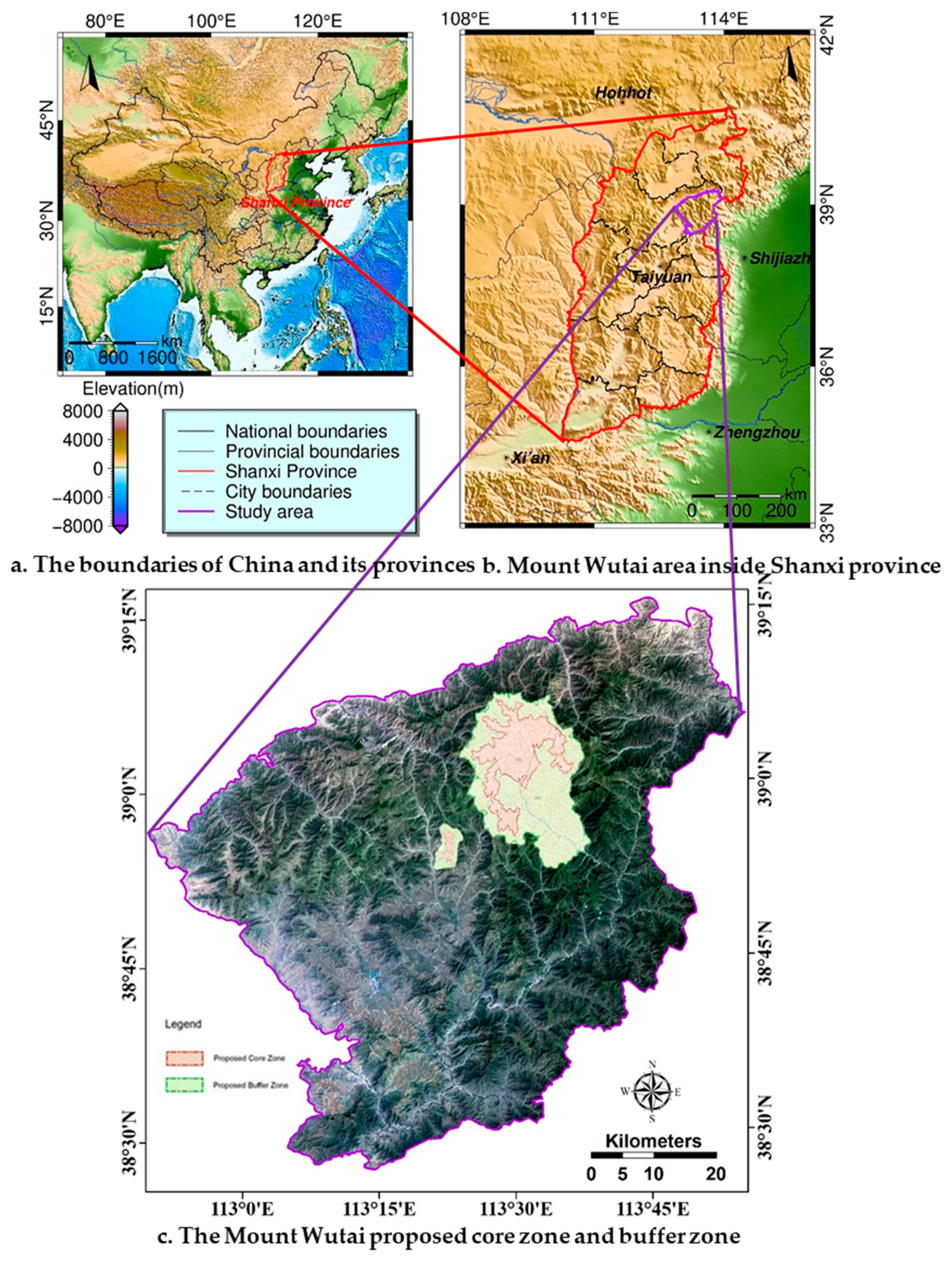
2.1. Study Area
2.2. Data
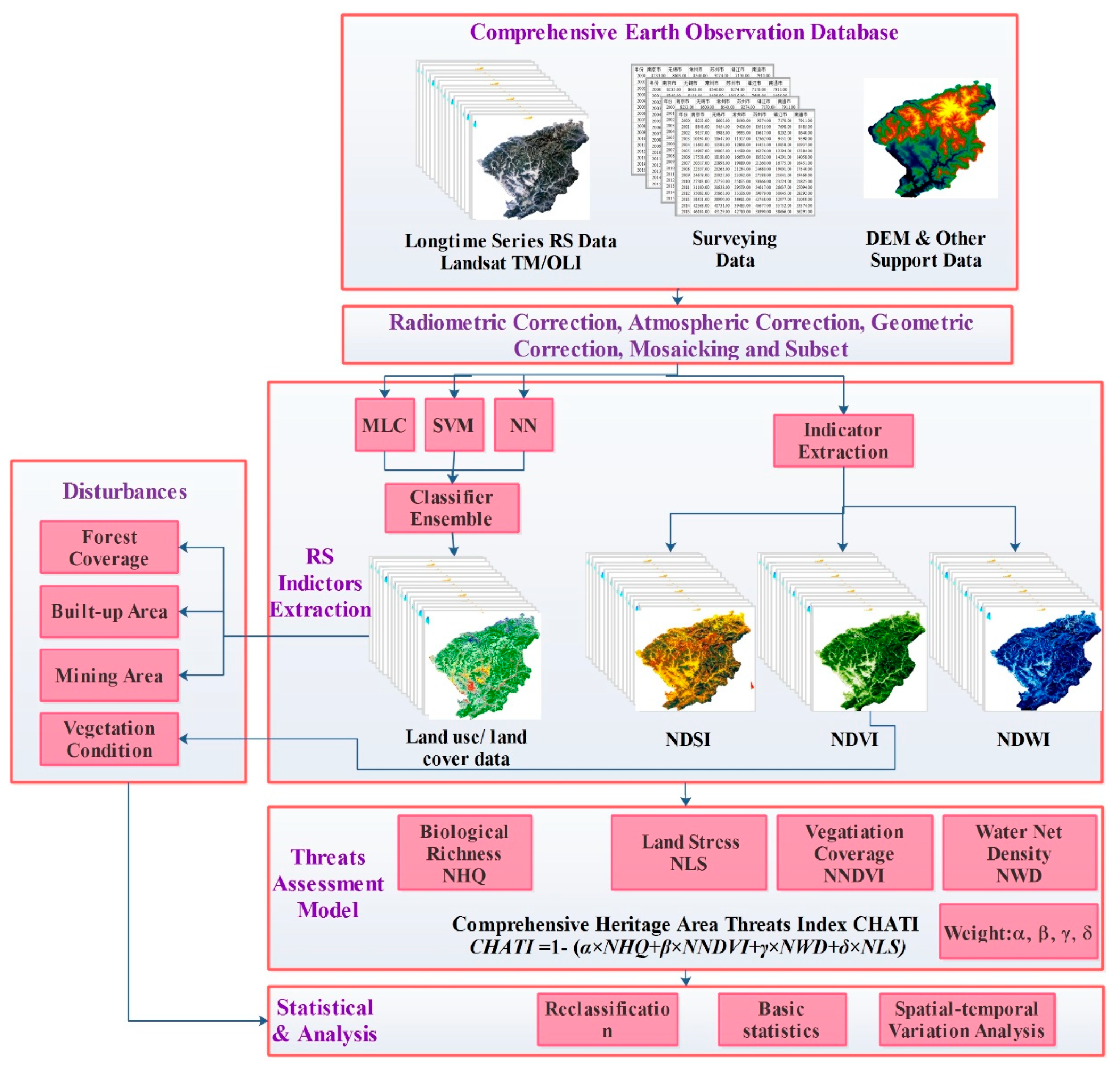
3. Method
3.1. LULC and Indices Extraction
3.2. Identification of Land Cover Disturbances
3.3. Comprehensive Assessment System of Threats in the Heritage Area.
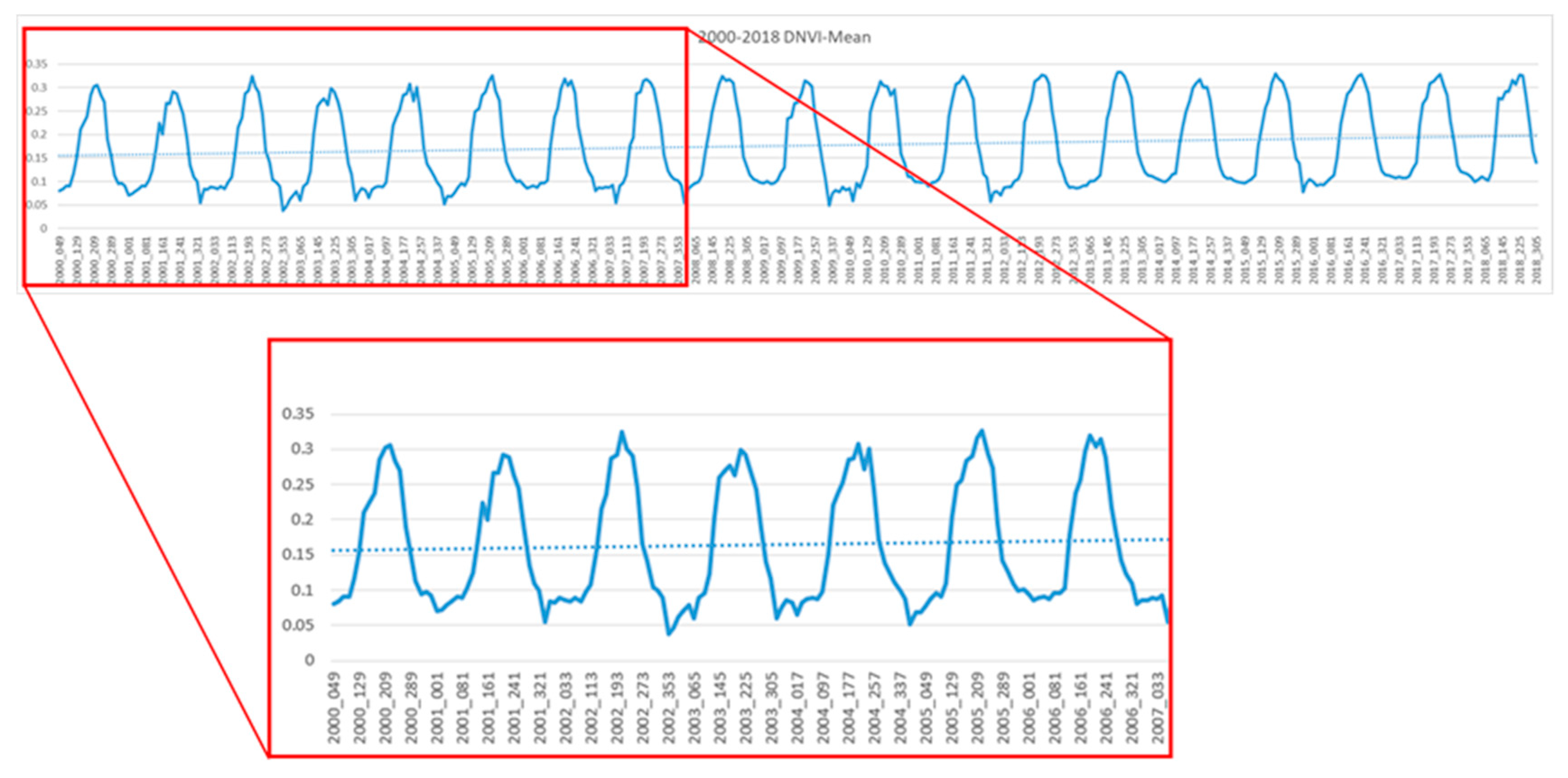
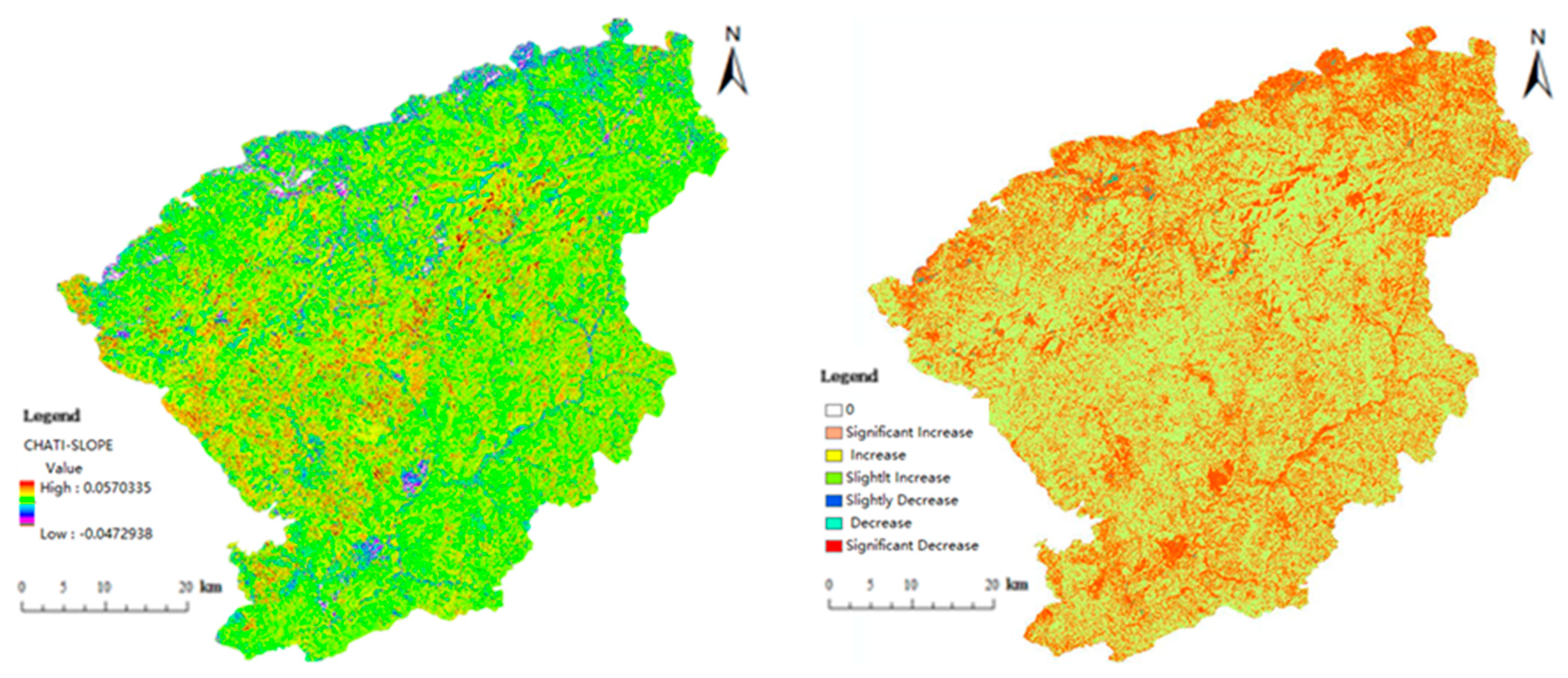
3.4. Variation Trends of NDVI and CHATI
4. Result and Analysis
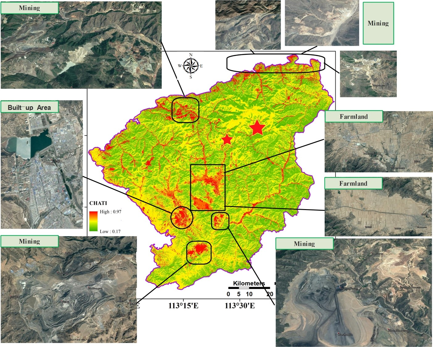
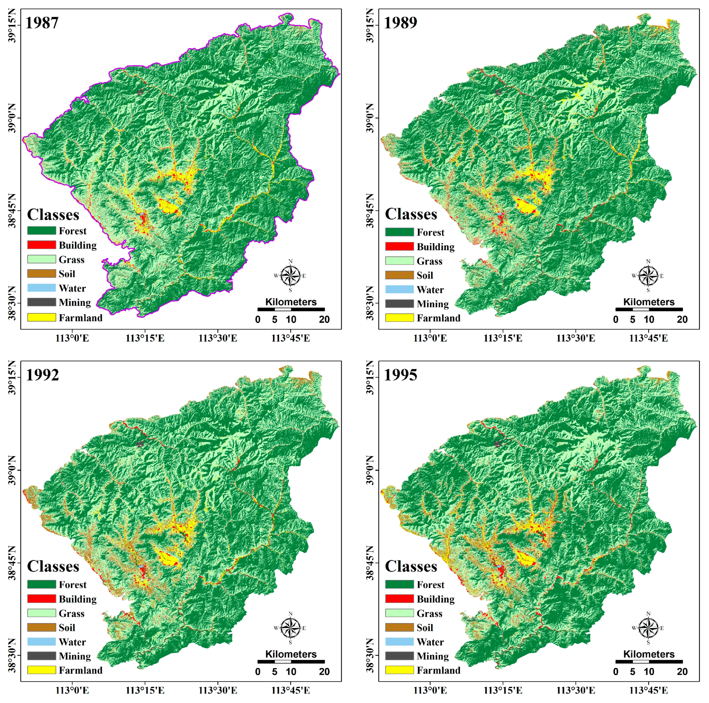
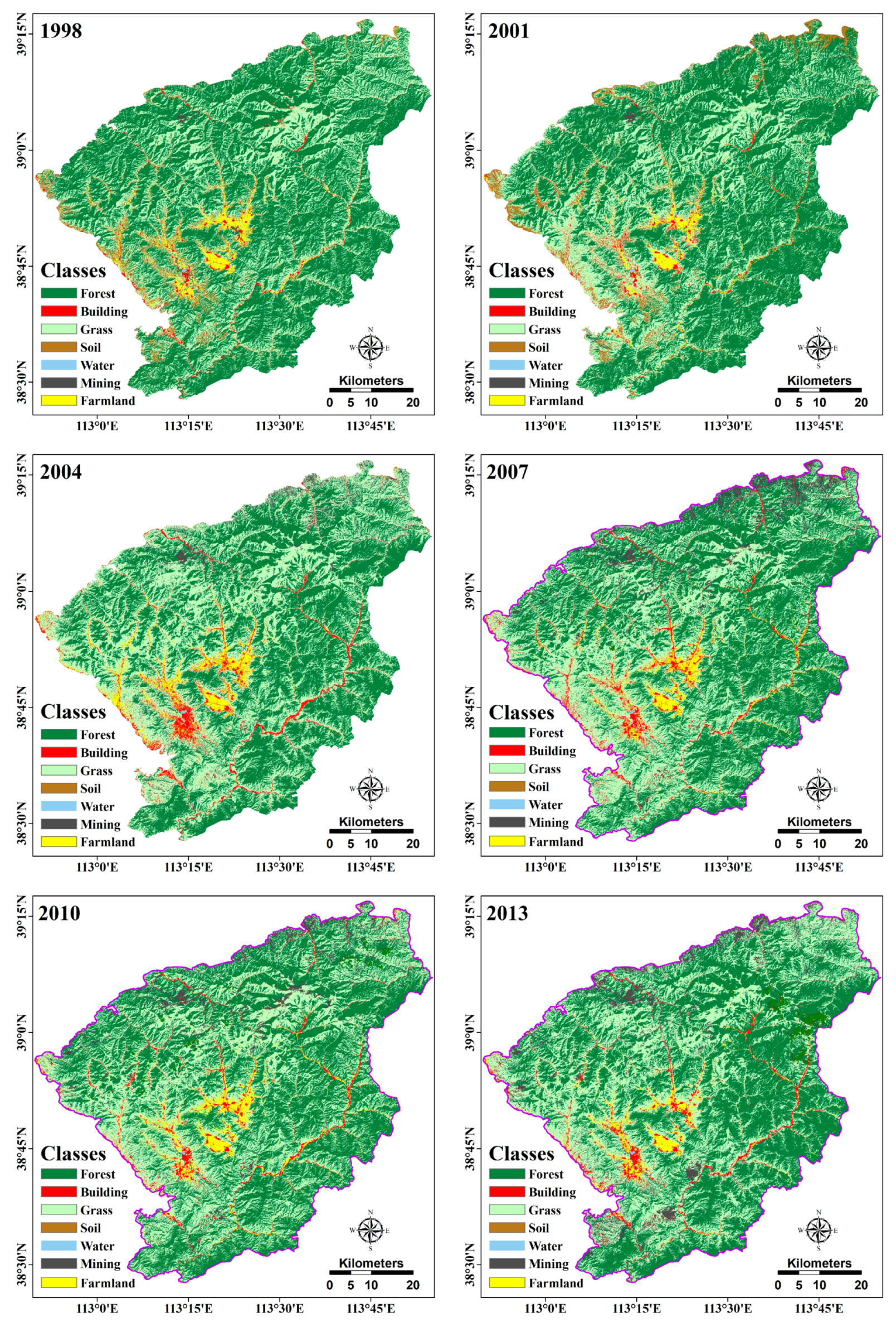
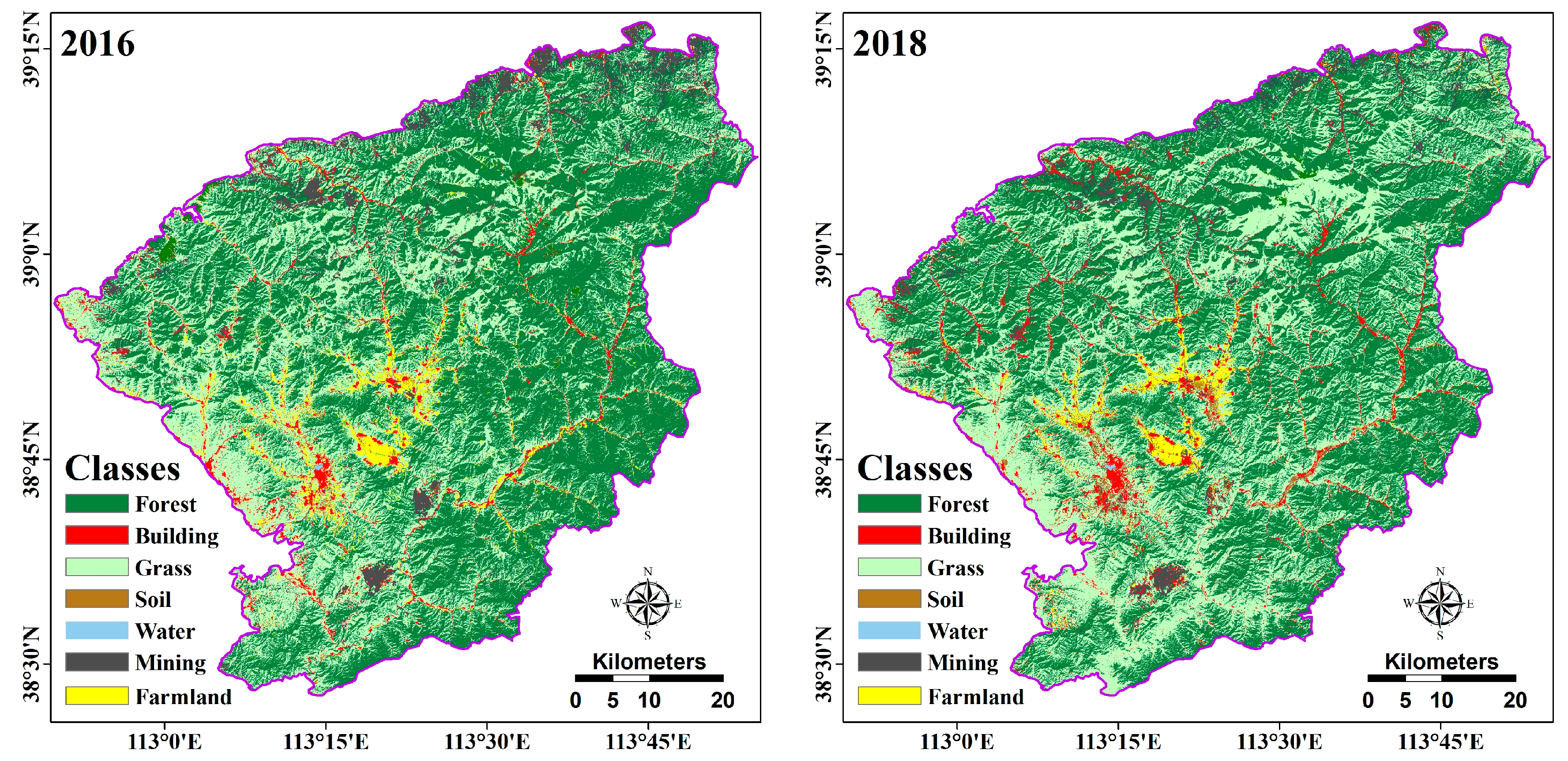
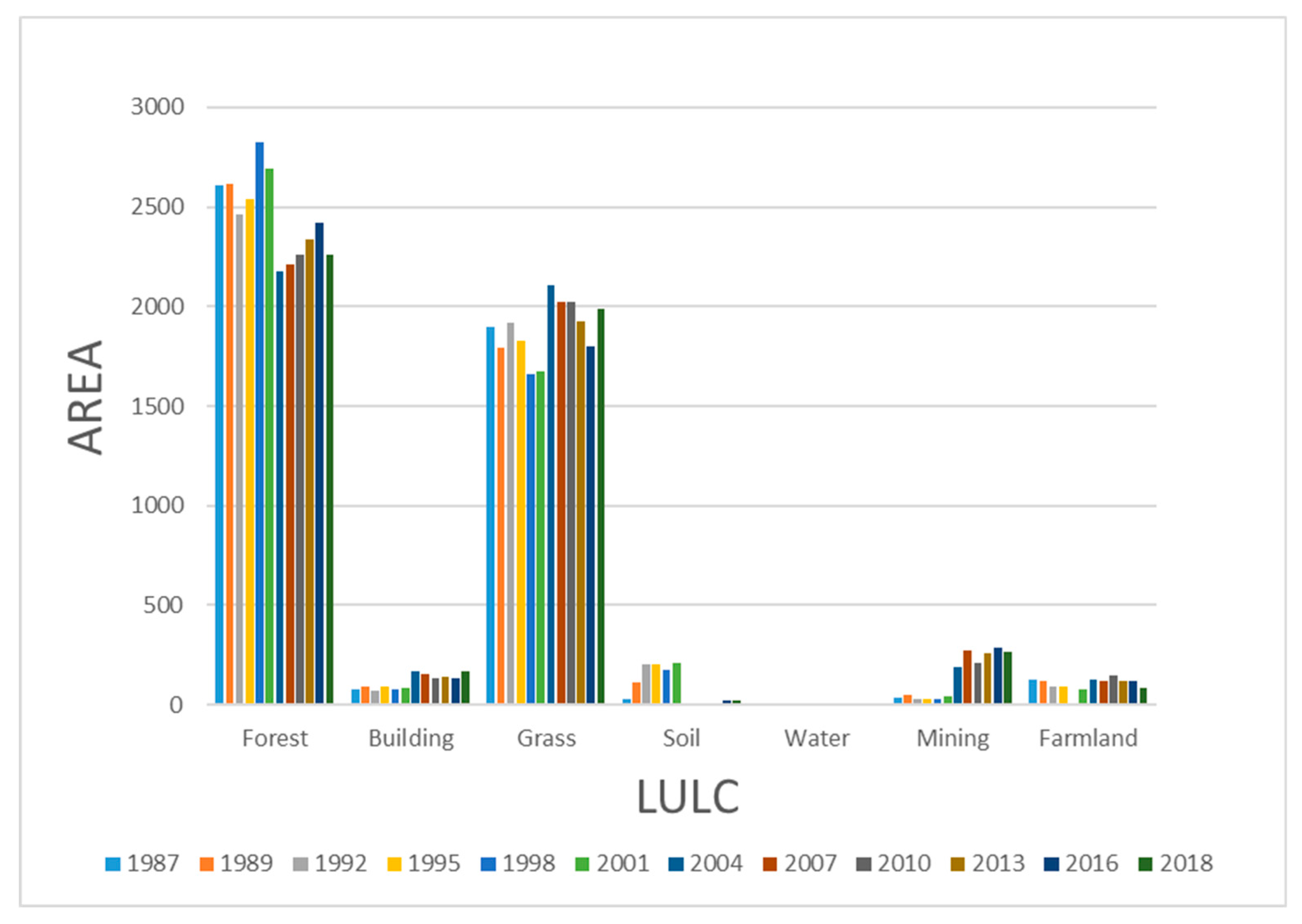
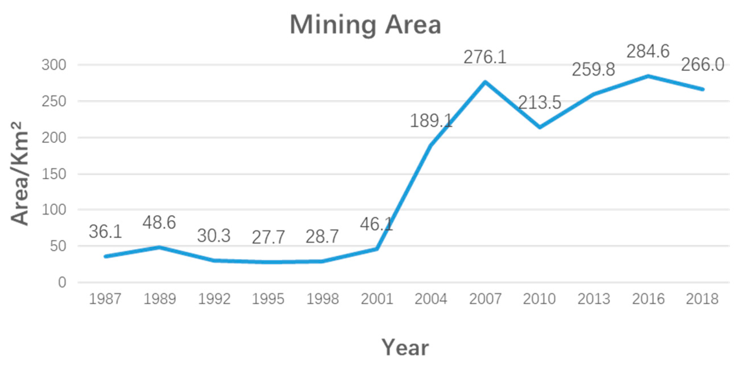
4.1. The Distribution and Variation of Main Disturbances
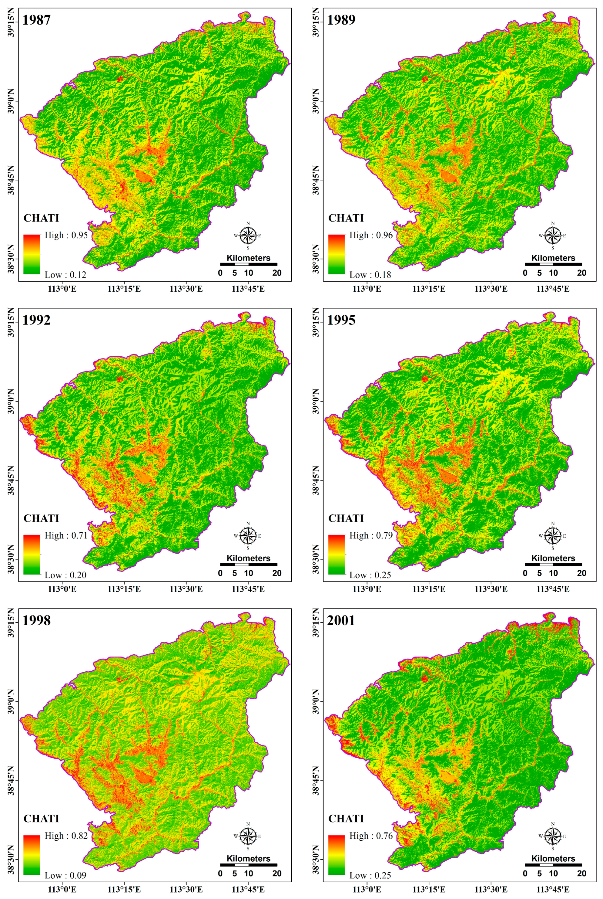
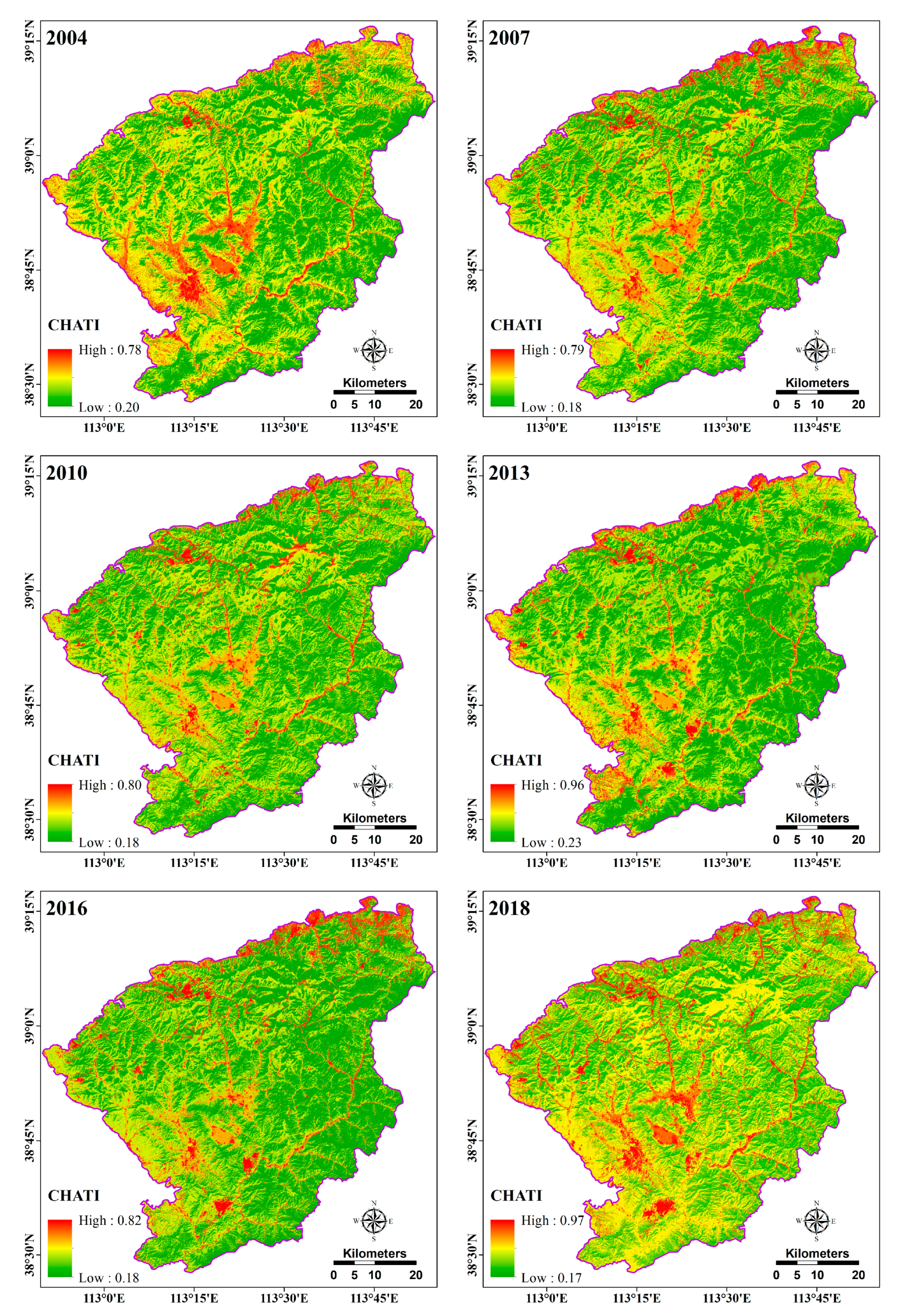
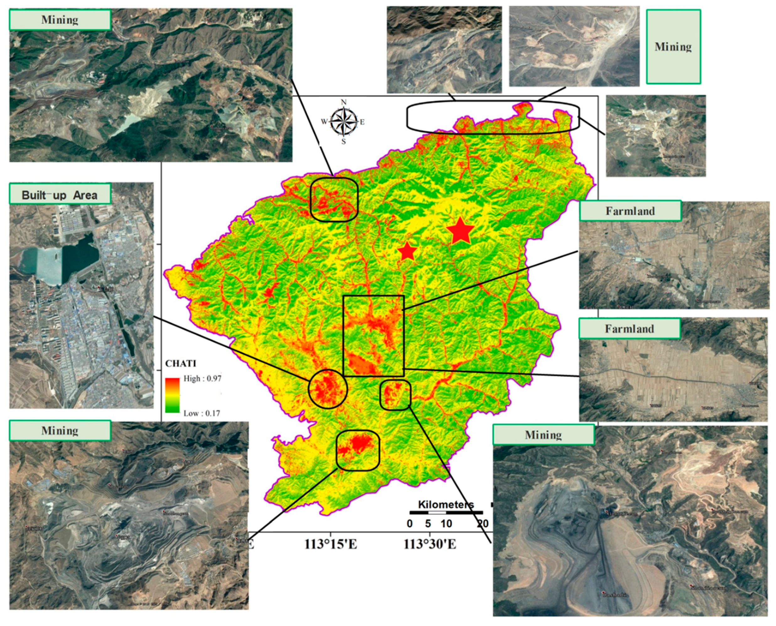
4.2. Comprehensive Heritage Threats Assessment Index
5. Conclusions
Author Contributions
Funding
Acknowledgments
Conflicts of Interest
References
- Poria, Y.; Reichel, A.; Cohen, R. Tourists perceptions of World Heritage Site and its designation. Tour. Manag. 2013, 35, 272–274. [Google Scholar] [CrossRef]
- Drost, A. Developing sustainable tourism for world heritage sites. Ann. Tour. Res. 1996, 23, 479–484. [Google Scholar] [CrossRef]
- Leask, A.; Fyall, A. Managing World Heritage Sites; Routledge: Abingdon, UK, 2006. [Google Scholar]
- Rössler, M. World heritage cultural landscapes: A UNESCO flagship programme 1992–2006. Landsc. Res. 2006, 31, 333–353. [Google Scholar] [CrossRef]
- UNESCO World Heritage Centre. The Criteria for Selection; UNESCO World Heritage Centre: Paris, France, 2011. [Google Scholar]
- Agapiou, A.; Lysandrou, V.; Alexakis, D.D.; Themistocleous, K.; Cuca, B.; Argyriou, A.; Sarris, A.; Hadjimitsis, D.G. Cultural heritage management and monitoring using remote sensing data and GIS: The case study of Paphos area, Cyprus. Comput. Environ. Urban Syst. 2015, 54, 230–239. [Google Scholar] [CrossRef]
- Cowley, D.C. Remote Sensing for Archaeological Heritage Management; Europae Archaeologia Consilium: Brussels, Belgium, 2011. [Google Scholar]
- Watson, J.E.M.; Dudley, N.; Segan, D.B.; Hockings, M. The performance and potential of protected areas. Nature. 2014, 515, 67–73. [Google Scholar] [CrossRef]
- Voogt, J.A.; Oke, T.R. Thermal remote sensing of urban climates. Remote Sens. Environ. 2003, 86, 370–384. [Google Scholar] [CrossRef]
- Pappu, S.; Akhilesh, K.; Ravindranath, S.; Raj, U. Applications of satellite remote sensing for research and heritage management in Indian prehistory. J. Archaeol. Sci. 2010, 37, 2316–2331. [Google Scholar] [CrossRef]
- Nagendra, H.; Lucas, R.; Honrado, J.P.; Jongman, R.H.G.; Tarantino, C.; Adamo, M.; Mairota, P. Remote sensing for conservation monitoring: Assessing protected areas, habitat extent, habitat condition, species diversity, and threats. Ecol. Indic. 2013, 33, 45–59. [Google Scholar] [CrossRef]
- Willis, K.S. Remote sensing change detection for ecological monitoring in United States protected areas. Biol. Conserv. 2015, 182, 233–242. [Google Scholar] [CrossRef]
- Rykiel, E.J. Towards a definition of ecological disturbance. Aust. J. Ecol. 1985, 10, 361–365. [Google Scholar] [CrossRef]
- Brimblecombe, P.; Grossi, C.M.; Harris, I. Climate change critical to cultural heritage. In Survival and Sustainability; Springer: Berlin, Germany, 2010; pp. 195–205. [Google Scholar]
- West, P.; Igoe, J.; Brockington, D. Parks and peoples: The social impact of protected areas. Annu. Rev. Anthropol. 2006, 35, 251–277. [Google Scholar] [CrossRef]
- Frey, B.S.; Steiner, L. World Heritage List: Does it make sense? Int. J. Cult. Policy 2011, 17, 555–573. [Google Scholar] [CrossRef]
- Gross, J.E.; Goetz, S.J.; Cihlar, J. Application of remote sensing to parks and protected area monitoring: Introduction to the special issue. Remote Sens. Environ. 2009, 113, 1343–1345. [Google Scholar] [CrossRef]
- Ali, S.H. Mining, the Environment, and Indigenous Development Conflicts; University of Arizona Press: Tucson, AZ, USA, 2009. [Google Scholar]
- Rice, J.; Trujillo, V.; Jennings, S.; Hylland, K.; Hagstrom, O.; Astudillo, A.; Jensen, J.N. Guidance on the Application of the Ecosystem Approach to Management of Human Activities in the European Marine Environment. Available online: https://www.researchgate.net/publication/230659987_Guidance_on_the_Application_of_the_Ecosystem_Approach_to_Management_of_Human_Activities_in_the_European_Marine_Environment (accessed on 30 May 2019).
- Xu, X.; Yang, G.; Tan, Y.; Zhuang, Q.; Li, H.; Wan, R.; Su, W.; Zhang, J. Ecological risk assessment of ecosystem services in the Taihu Lake Basin of China from 1985 to 2020. Sci. Total Environ. 2016, 554, 7–16. [Google Scholar] [CrossRef] [PubMed]
- Maekawa, M.; Lanjouw, A.; Rutagarama, E.; Sharp, D. Mountain gorilla tourism generating wealth and peace in post-conflict R wanda. Nat. Resour. Forum 2013, 37, 127–137. [Google Scholar] [CrossRef]
- Kennedy, R.; Yang, Z.; Braaten, J.; Neldon, P.; Cohen, W. Monitoring landscape dynamics of National Parks in the western United States. In Remote Sensing of Protected Lands; CRC Press: Boca Raton, FL, USA, 2012; pp. 57–75. [Google Scholar]
- Wiens, J.; Sutter, R.; Anderson, M.; Blanchard, J.; Barnett, A.; Aguilar-Amuchastegui, N.; Avery, C.; Laine, S. Selecting and conserving lands for biodiversity: The role of Remote Sensing. Remote Sens. Environ. 2009, 113, 1370–1381. [Google Scholar] [CrossRef]
- Dennison, P.E.; Nagler, P.L.; Hultine, K.R.; Glenn, E.P.; Ehleringer, J.R. Remote monitoring of tamarisk defoliation and evapotranspiration following saltcedar leaf beetle attack. Remote Sens. Environ. 2009, 113, 1462–1472. [Google Scholar] [CrossRef]
- Jones, J.W.; Hall, A.E.; Foster, A.M.; Smith, T.J. Wetland fire scar monitoring and analysis using archival Landsat data for the Everglades. Fire Ecol. 2013, 9, 133–150. [Google Scholar] [CrossRef]
- Munns, W.J.E. Society. Assessing risks to wildlife populations from multiple stressors: Overview of the problem and research needs. Ecol. Soc. 2006, 11, 23. [Google Scholar] [CrossRef]
- Feng, Y.; Liu, Y.; Liu, Y. Assessment, R. Spatially explicit assessment of land ecological security with spatial variables and logistic regression modeling in Shanghai, China. Stoch. Environ. Res. Risk Assess. 2017, 31, 2235–2249. [Google Scholar] [CrossRef]
- DeFries, R.; Hansen, A.; Newton, A.C.; Hansen, M.C. Increasing isolation of protected areas in tropical forests over the past twenty years. Ecol. Appl. 2005, 15, 19–26. [Google Scholar] [CrossRef]
- Ingram, J.C.; Dawson, T.P.; Whittaker, R.J. Mapping tropical forest structure in southeastern Madagascar using remote sensing and artificial neural networks. Remote Sens. Environ. 2005, 94, 491–507. [Google Scholar] [CrossRef]
- Nunes, M.C.; Vasconcelos, M.J.; Pereira, J.M.; Dasgupta, N.; Alldredge, R.J.; Rego, F.C. Land cover type and fire in Portugal: Do fires burn land cover selectively? Landsc. Ecol. 2005, 20, 661–673. [Google Scholar] [CrossRef]
- Fuller, D.O. Tropical forest monitoring and remote sensing: A new era of transparency in forest governance? Singap. J. Trop. Geogr. 2006, 27, 15–29. [Google Scholar] [CrossRef]
- Nagendra, H.; Pareeth, S.; Sharma, B.; Schweik, C.M.; Adhikari, K.R. Forest fragmentation and regrowth in an institutional mosaic of community, government and private ownership in Nepal. Landsc. Ecol. 2008, 23, 41–54. [Google Scholar] [CrossRef]
- Nagendra, H.; Rocchini, D.; Ghate, R.; Sharma, B.; Pareeth, S. Assessing plant diversity in a dry tropical forest: Comparing the utility of Landsat and IKONOS satellite images. Remote Sens. 2010, 2, 478–496. [Google Scholar] [CrossRef]
- Luo, J.; Du, P.; Samat, A.; Xia, J.; Che, M.; Xue, Z. Spatiotemporal Pattern of PM2.5 Concentrations in Mainland China and Analysis of Its Influencing Factors using Geographically Weighted Regression. Sci. Rep. 2017, 7, 40607. [Google Scholar] [CrossRef] [PubMed]
- Du, P.; Xia, J.; Zhang, W.; Tan, K.; Liu, Y.; Liu, S. Multiple classifier system for remote sensing image classification: A review. Sensors 2012, 12, 4764–4792. [Google Scholar] [CrossRef]
- Du, P.; Samat, A.; Waske, B.; Liu, S.; Li, Z. Random forest and rotation forest for fully polarized SAR image classification using polarimetric and spatial features. ISPRS J. Photogramm. Remote Sens. 2015, 105, 38–53. [Google Scholar] [CrossRef]
- Du, P.; Liu, S.; Xia, J.; Zhao, Y. Information fusion techniques for change detection from multi-temporal remote sensing images. Inf. Fusion 2013, 14, 19–27. [Google Scholar] [CrossRef]
- Pôças, I.; Cunha, M.; Pereira, L.S. Remote sensing based indicators of changes in a mountain rural landscape of Northeast Portugal. Appl. Geogr. 2011, 31, 871–880. [Google Scholar] [CrossRef]
- Gitelson, A.A.; Merzlyak, M.N. Signature analysis of leaf reflectance spectra: Algorithm development for remote sensing of chlorophyll. J. Plant Physiol. 1996, 148, 494–500. [Google Scholar] [CrossRef]
- Liu, Y.; Sarnat, J.A.; Kilaru, V.; Jacob, D.J.; Koutrakis, P. Estimating ground-level PM2. 5 in the eastern United States using satellite Remote Sensing. Environ. Sci. Technol. 2005, 39, 3269–3278. [Google Scholar] [CrossRef]
- Van Donkelaar, A.; Martin, R.V.; Park, R.J. Estimating ground-level PM2. 5 using aerosol optical depth determined from satellite Remote Sens. J. Geophys. Res. Atmos. 2006, 111. [Google Scholar] [CrossRef]
- Kimes, D.; Sellers, P.J. Inferring hemispherical reflectance of the Earth’s surface for global energy budgets from remotely sensed nadir or directional radiance values. Remote Sens. Environ. 1985, 18, 205–223. [Google Scholar] [CrossRef]
- Bastiaanssen, W.G.; Menenti, M.; Feddes, R.; Holtslag, A.A.M. A remote sensing surface energy balance algorithm for land (SEBAL). 1. Formulation. J. Hydrol. 1998, 212, 198–212. [Google Scholar] [CrossRef]
- Jackson, T.J., III. Measuring surface soil moisture using passive microwave Remote Sensing. Hydrol. Process. 1993, 7, 139–152. [Google Scholar] [CrossRef]
- Weng, Q. A remote sensing? GIS evaluation of urban expansion and its impact on surface temperature in the Zhujiang Delta, China. Int. J. Remote Sens. 2001, 22, 1999–2014. [Google Scholar]
- Gao, B.-C. NDWI—A normalized difference water index for remote sensing of vegetation liquid water from space. Remote Sens. Environ. 1996, 58, 257–266. [Google Scholar] [CrossRef]
- Bai, Z.; Dent, D.; Olsson, L.; Schaepman, M. Global Assessment of Land Degradation and impRovement: 1. Identification by Remote Sensing; ISRIC-World Soil Information: Wageningen, The Netherlands, 2008. [Google Scholar]
- Curran, P. Multispectral remote sensing of vegetation amount. Prog. Phys. Geogr. 1980, 4, 315–341. [Google Scholar] [CrossRef]
- Lu, D. The potential and challenge of remote sensing-based biomass estimation. Int. J. Remote Sens. 2006, 27, 1297–1328. [Google Scholar] [CrossRef]
- Ruimy, A.; Saugier, B.; Dedieu, G. Methodology for the estimation of terrestrial net primary production from remotely sensed data. J. Geophys. Res. Atmos. 1994, 99, 5263–5283. [Google Scholar] [CrossRef]
- Field, C.B.; Randerson, J.T.; Malmström, C.M. Global net primary production: Combining ecology and Remote Sensing. Remote Sens. Environ. 1995, 51, 74–88. [Google Scholar] [CrossRef]
- Lefsky, M.A.; Cohen, W.B.; Parker, G.G.; Harding, D. J Lidar remote sensing for ecosystem studies: Lidar, an emerging remote sensing technology that directly measures the three-dimensional distribution of plant canopies, can accurately estimate vegetation structural attributes and should be of particular interest to forest, landscape, and global ecologists. BioScience 2002, 52, 19–30. [Google Scholar]
- Dandois, J.P.; Ellis, E.C. Remote sensing of vegetation structure using computer vision. Remote Sens. 2010, 2, 1157–1176. [Google Scholar] [CrossRef]
- Kerr, J.T.; Ostrovsky, M. From space to species: Ecological applications for Remote Sensing. Trends Ecol. Evol. 2003, 18, 299–305. [Google Scholar] [CrossRef]
- Quattrochi, D.A.; Luvall, J.C. Thermal infrared remote sensing for analysis of landscape ecological processes: Methods and applications. Landsc. Ecol. 1999, 14, 577–598. [Google Scholar] [CrossRef]
- Van Donkelaar, A.; Martin, R.V.; Brauer, M.; Hsu, N.C.; Kahn, R.A.; Levy, R.C.; Lyapustin, A.; Sayer, A.M.; Winker, D.M. Global estimates of fine particulate matter using a combined geophysical-statistical method with information from satellites, models, and monitors. Environ. Sci. Technol. 2016, 50, 3762–3772. [Google Scholar] [CrossRef]
- Zheng, Y.; Zhang, Q.; Liu, Y.; Geng, G.; He, K. Estimating ground-level PM2. 5 concentrations over three megalopolises in China using satellite-derived aerosol optical depth measurements. Atmos. Environ. 2016, 124, 232–242. [Google Scholar] [CrossRef]
- Guo, Y.; Tang, Q.; Gong, D.-Y.; Zhang, Z. Estimating ground-level PM2. 5 concentrations in Beijing using a satellite-based geographically and temporally weighted regression model. Remote Sens. Environ. 2017, 198, 140–149. [Google Scholar] [CrossRef]
- Simic, A.; Chen, J.M.; Liu, J.; Csillag, F. Spatial scaling of net primary productivity using subpixel information. Remote Sens. Environ. 2004, 93, 246–258. [Google Scholar] [CrossRef]
- Bian, J.-H.; Li, A.; Song, M.; Ma, L.; Jiang, J. Reconstruction of NDVI time-series datasets of MODIS based on Savitzky-Golay filter. J. Remote Sens. 2010, 14, 725–741. [Google Scholar]
- Lu, D.; Xu, X.; Tian, H.; Moran, E.; Zhao, M.; Running, S. The effects of urbanization on net primary productivity in southeastern China. Environ. Manag. 2010, 46, 404–410. [Google Scholar] [CrossRef] [PubMed]
- Xu, H.; Wang, M.; Shi, T.; Guan, H.; Fang, C.; Lin, Z. Prediction of ecological effects of potential population and impervious surface increases using a remote sensing based ecological index (RSEI). Ecol. Indic. 2018, 93, 730–740. [Google Scholar] [CrossRef]
- Srinivasa Rao, Y.; Jugran, D.K. Delineation of groundwater potential zones and zones of groundwater quality suitable for domestic purposes using remote sensing and GIS. Hydrol. Sci. J. 2003, 48, 821–833. [Google Scholar] [CrossRef]
- Miller, R.B.; Small, C. Cities from space: Potential applications of remote sensing in urban environmental research and policy. Environ. Sci. Policy 2003, 6, 129–137. [Google Scholar] [CrossRef]
- Luo, J.; Zhou, T.; Du, P.; Xu, Z. Spatial-temporal variations of natural suitability of human settlement environment in the Three Gorges Reservoir Area—A case study in Fengjie County, China. Front. Earth Sci. 2019, 13, 1–17. [Google Scholar] [CrossRef]
- Yinkang, C.F.; Feng, Z. Analysis of the spatial distribution pattern of urban land price with geostatistics. J. Naijing Univ. Nat. Sci. 1999, 6, 719–723. [Google Scholar]
- Luo, J.; Du, P.; Samat, A.; Feng, L. Evaluation on the natural suitability of urban human settlement environment using multisource data. In Proceedings of the 2015 Joint Urban Remote Sensing Event (JURSE), Lausanne, Switzerland, 30 March–1 April 2015; pp. 1–4. [Google Scholar]
- Patino, J.E.; Duque, J.C.; Pardo-Pascual, J.E.; Ruiz, L.A. Using remote sensing to assess the relationship between crime and the urban layout. Appl. Geogr. 2014, 55, 48–60. [Google Scholar] [CrossRef]
- Xu, Z.; Li, Q. Integrating the empirical models of benchmark land price and GIS technology for sustainability analysis of urban residential development. Habitat Int. 2014, 44, 79–92. [Google Scholar] [CrossRef]
- Xu, Y.; Sun, J.; Zhang, J.; Xu, Y.; Zhang, M.; Liao, X. Combining AHP with GIS in synthetic evaluation of environmental suitability for living in China’s 35 major cities. Int. J. Geogr. Inf. Sci. 2012, 26, 1603–1623. [Google Scholar] [CrossRef]
- Ouzounis, G.K.; Syrris, V.; Pesaresi, M. Multiscale quality assessment of Global Human Settlement Layer scenes against reference data using statistical learning. Pattern Recognit. Lett. 2013, 34, 1636–1647. [Google Scholar] [CrossRef]
- Shen, L.; Kyllo, J.; Guo, X. An integrated model based on a hierarchical indices system for monitoring and evaluating urban sustainability. Sustainability 2013, 5, 524–559. [Google Scholar] [CrossRef]
- Xu, C.; Liu, M.; An, S.; Chen, J.; Yan, P. Assessing the impact of urbanization on regional net primary productivity in Jiangyin County, China. J. Environ. Manag. 2007, 85, 597–606. [Google Scholar] [CrossRef] [PubMed]
- Wu, C.; Murray, A.T. Estimating impervious surface distribution by spectral mixture analysis. Remote Sens. Environ. 2003, 84, 493–505. [Google Scholar] [CrossRef]
- Du, H.; Cai, W.; Xu, Y.; Wang, Z.; Wang, Y.; Cai, Y. Quantifying the cool island effects of urban green spaces using remote sensing Data. Urban For. Urban Green. 2017, 27, 24–31. [Google Scholar] [CrossRef]
- Du, P.; Bai, X.; Luo, J.; Li, E.; Lin, C. Advances of urban Remote Sensing. Nanjing Xinxi Gongcheng Daxue Xuebao 2018, 10, 16–29. [Google Scholar]
- Li, S.; Zhao, G.; Wilde, S.A.; Zhang, J.; Sun, M.; Zhang, G.; Dai, L. Deformation history of the Hengshan–Wutai–Fuping Complexes: Implications for the evolution of the Trans-North China Orogen. Gondwana Res. 2010, 18, 611–631. [Google Scholar] [CrossRef]
- Liu, S.; Pan, Y.; Xie, Q.; Zhang, J.; Li, Q. Archean geodynamics in the Central Zone, North China Craton: Constraints from geochemistry of two contrasting series of granitoids in the Fuping and Wutai complexes. Precambrian Res. 2004, 130, 229–249. [Google Scholar] [CrossRef]
- Stevenson, D. Visions of Mañjuśrī on Mount Wutai. Relig. China Pract. 1996, 3, 203. [Google Scholar]
- Lin, W.-C. Building a Sacred Mountain: The Buddhist Architecture of China’s Mount Wutai; University of Washington Press: Seattle, WA, USA, 2014. [Google Scholar]
- Ryan, C.; Gu, H. Constructionism and culture in research: Understandings of the fourth Buddhist Festival, Wutaishan, China. Tour. Manag. 2010, 31, 167–178. [Google Scholar] [CrossRef]
- Wang, K.; Li, J.; Hao, J.; Li, J.; Shaoping, Z. The Wutaishan orogenic belt within the Shanxi Province, northern China: A record of late Archaean collision tectonics. Precambrian Res. 1996, 78, 95–103. [Google Scholar] [CrossRef]
- Wutai Bureau of Statistics of Wutai County. Yearbook; Wutai Bureau of Statistics of Wutai County: Xinzhou, China, 2010. [Google Scholar]
- Wutai Bureau of Statistics of Wutai County. Yearbook; Wutai Bureau of Statistics of Wutai County: Xinzhou, China, 2013. [Google Scholar]
- Zhang, W.; Wang, J. School of Tourism Management, Xiangtan University; On Development of Red Tourism Resources in China—Taking Wutai County in Shanxi Province as an Example. J. Hunan Univ. Technol. Soc. Sci. Ed. 2013, 4, 9. [Google Scholar]
- Thenkabail, P.S.; Schull, M.; Turral, H. Ganges and Indus river basin land use/land cover (LULC) and irrigated area mapping using continuous streams of MODIS data. Remote Sens. Environ. 2005, 95, 317–341. [Google Scholar] [CrossRef]
- Yang, X.; Huang, Y.; Dong, P.; Jiang, D.; Liu, H. An updating system for the gridded population database of China based on remote sensing, GIS and spatial database technologies. Sensors 2009, 9, 1128–1140. [Google Scholar] [CrossRef] [PubMed]
- Mengistu, D.A.; Salami, A.T. Technology. Application of remote sensing and GIS inland use/land cover mapping and change detection in a part of south western Nigeria. Afr. J. Environ. Sci. Technol. 2007, 1, 99–109. [Google Scholar]
- Alo, C.A.; Pontius, R.G., Jr. Identifying systematic land-cover transitions using remote sensing and GIS: The fate of forests inside and outside protected areas of Southwestern Ghana. Environ. Plan. B Plan. Des. 2008, 35, 280–295. [Google Scholar] [CrossRef]
- Liu, J.; Linderman, M.; Ouyang, Z.; An, L.; Yang, J.; Zhang, H. Ecological degradation in protected areas: The case of Wolong Nature Reserve for giant pandas. Science 2001, 292, 98–101. [Google Scholar] [CrossRef] [PubMed]
- Kairo, J.G.; Kivyatu, B.; Koedam, N. Application of Remote Sensing and GIS in the Management of Mangrove Forests Within and Adjacent to Kiunga Marine Protected Area, Lamu, Kenya. Environ. Dev. Sustain. 2002, 4, 153–166. [Google Scholar] [CrossRef]
- Running, S.W. Estimating terrestrial primary productivity by combining remote sensing and ecosystem simulation. In Remote Sensing of Biosphere Functioning; Springer: Berlin, Germany, 1990; pp. 65–86. [Google Scholar]
- Myneni, R.B.; Hall, F.G.; Sellers, P.J.; Marshak, A.L. The interpretation of spectral vegetation indexes. IEEE Trans. Geosci. Remote Sens. 1995, 33, 481–486. [Google Scholar] [CrossRef]
- Han-Qiu, X.U. A Study on Information Extraction of Water Body with the Modified Normalized Difference Water Index (MNDWI). J. Remote Sens. 2005, 5, 589–595. [Google Scholar]
- Zhou, C.-L.; Xu, H.-Q. A Spectral Mixture Analysis and Mapping of Impervious Surfaces in Built-up Land of Fuzhou City. J. Image Graph. 2007, 5, 875–881. [Google Scholar]
- Xu, H. Assessment of ecological change in soil loss area using remote sensing technology. Trans. Chin. Soc. Agric. Eng. 2013, 29, 91–97. [Google Scholar]
- Xu, H. Fast information extraction of urban built-up land based on the analysis of spectral signature and normalized difference index. Geogr. Res. 2005, 24, 311–320. [Google Scholar]
- Xu, H. A new index for delineating built-up land features in satellite imagery. Int. J. Remote Sens. 2008, 29, 4269–4276. [Google Scholar] [CrossRef]
- Huete, A.R. A soil-adjusted vegetation index (SAVI). Remote Sens. Environ. 1988, 25, 295–309. [Google Scholar] [CrossRef]
- Zhu, G.; Liu, Y.; Ju, W.; Chen, J. Evaluation of topographic effects on four commonly used vegetation indices. Yaogan Xuebao-J. Remote Sens. 2013, 17, 210–234. [Google Scholar]
- Ministry of Ecology and Environment of the P.R.China. Technical Specifications for Evaluation of Ecological Environment Conditions; Ministry of Ecology and Environment of the P.R.China, Ed.; 2015. [Google Scholar]
- Seber, G.A.; Lee, A.J. Linear Regression Analysis; John Wiley & Sons: Hoboken, NJ, USA, 2012; Volume 329. [Google Scholar]
- Lix, L.M.; Keselman, J.C.; Keselman, H. Consequences of assumption violations revisited: A quantitative review of alternatives to the one-way analysis of variance F test. Rev. Educ. Res. 1996, 66, 579–619. [Google Scholar] [CrossRef]
- Tripathy, G.; Ghosh, T.; Shah, S.D. Monitoring of desertification process in Karnataka state of India using multi-temporal remote sensing and ancillary information using GIS. Int. J. Remote Sens. 1996, 17, 2243–2257. [Google Scholar] [CrossRef]
- Seto, K.C.; Kaufmann, R.K. Modeling the drivers of urban land use change in the Pearl River Delta, China: Integrating remote sensing with socioeconomic data. Land Econ. 2003, 79, 106–121. [Google Scholar] [CrossRef]
- Johnson, L.; Bosch, D.; Williams, D.; Lobitz, B.M. Remote sensing of vineyard management zones: Implications for wine quality. Appl. Eng. Agric. 2001, 17, 557. [Google Scholar] [CrossRef]
- Johnson, B.A.; Iizuka, K. Integrating OpenStreetMap crowdsourced data and Landsat time-series imagery for rapid land use/land cover (LULC) mapping: Case study of the Laguna de Bay area of the Philippines. Appl. Geogr. 2016, 67, 140–149. [Google Scholar] [CrossRef]
- Belgiu, M.; Drǎguţ, L. Comparing supervised and unsupervised multiresolution segmentation approaches for extracting buildings from very high resolution imagery. ISPRS J. Photogramm. Remote Sens. 2014, 96, 67–75. [Google Scholar] [CrossRef] [Green Version]
- Al-Saady, Y.; Merkel, B.; Al-Tawash, B.; Al-Suhail, Q. Land use and land cover (LULC) mapping and change detection in the Little Zab River Basin (LZRB), Kurdistan Region, NE Iraq and NW Iran. FOG-Freib. Online Geosci. 2015, 43, 1–32. [Google Scholar]
- Cohen, J. A coefficient of agreement for nominal scales. Educ. Psychol. Meas. 1960, 20, 37–46. [Google Scholar] [CrossRef]
- Thomlinson, J.R.; Bolstad, P.V.; Cohen, W.B. Coordinating methodologies for scaling landcover classifications from site-specific to global: Steps toward validating global map products. Remote Sens. Environ. 1999, 70, 16–28. [Google Scholar] [CrossRef]
- Zhang, M. China’s Poor Regions: Rural-Urban. Migration, Poverty, Economic Reform and Urbanisation; Routledge: Abingdon, UK, 2004. [Google Scholar]
- Shanxi Bureau of statistics of Shanxi Province. Yearbook; Shanxi Bureau of statistics of Shanxi Province: Shanxi, China, 2018. [Google Scholar]
- Wutai Bureau of statistics of Wutai County. Yearbook; Wutai Bureau of Statistics of Wutai County: Xinzhou, China, 2005. [Google Scholar]
- Myneni, R.; Tucker, C.; Asrar, G.; Keeling, C.D. Interannual variations in satellite-sensed vegetation index data from 1981 to 1991. J. Geophys. Res. Atmos. 1998, 103, 6145–6160. [Google Scholar] [CrossRef] [Green Version]
- Wang, Y.P.; Murie, A. The process of commercialisation of urban housing in China. Urban Stud. 1996, 33, 971–989. [Google Scholar] [CrossRef]
- Chen, J.; Guo, F.; Wu, Y. One decade of urban housing reform in China: Urban housing price dynamics and the role of migration and urbanization, 1995–2005. Habitat Int. 2011, 35, 1–8. [Google Scholar] [CrossRef]
- Logan, J.R.; Fang, Y.; Zhang, Z. The winners in China’s urban housing reform. Hous. Stud. 2010, 25, 101–117. [Google Scholar] [CrossRef]
- Wutai Bureau of statistics of Wutai County. Yearbook; Wutai Bureau of Statistics of Wutai County: Xinzhou, China, 2018. [Google Scholar]
- Wutai Bureau of statistics of Wutai County. Yearbook; Wutai Bureau of Statistics of Wutai County: Xinzhou, China, 2014. [Google Scholar]
- Xue, L.; Wang, M.Y.; Xue, T. ‘Voluntary’poverty alleviation resettlement in China. Dev. Chang. 2013, 44, 1159–1180. [Google Scholar] [CrossRef]
- Tu, J. Coal mining safety: China’s Achilles’ heel. China Secur. 2007, 3, 36–53. [Google Scholar]
- Cao, X. Policy and regulatory responses to coalmine closure and coal resources consolidation for sustainability in Shanxi, China. J. Clean. Prod. 2017, 145, 199–208. [Google Scholar] [CrossRef]
- Gao, H.Q.; Xiong, Y.Z.; Hu, S.W. World Financial Crisis and Its Impact on China. Stud. Int. Financ. 2008, 11. [Google Scholar]
- Zhang, J.; Fu, M.; Geng, Y.; Tao, J. Energy saving and emission reduction: A project of coal-resource integration in Shanxi Province, China. Energy Policy 2011, 39, 3029–3032. [Google Scholar] [CrossRef]
- Xie, H.; Wang, J.; Shen, B.; Liu, J.; Jiang, P.; Zhou, H.; Liu, H.; Wu, G. New idea of coal mining: Scientific mining and sustainable mining capacity. J. China Coal Soc. 2012, 37, 1069–1079. [Google Scholar]
- Metternicht, G.; Zinck, J.A. Remote sensing of soil salinity: Potentials and constraints. Remote Sens. Environ. 2003, 85, 1–20. [Google Scholar] [CrossRef]
- Fang, B.; Lakshmi, V. Soil moisture at watershed scale: Remote sensing techniques. J. Hydrol. 2014, 516, 258–272. [Google Scholar] [CrossRef]


| Jan | Feb | Mar | Apr | May | June | July | Aug | Sept | Oct | Nov | Dec | |
|---|---|---|---|---|---|---|---|---|---|---|---|---|
| 2018 | OLI | |||||||||||
| 2016 | OLI | |||||||||||
| 2013 | OLI | |||||||||||
| 2010 | TM | |||||||||||
| 2007 | TM | |||||||||||
| 2004 | TM | |||||||||||
| 2001 | TM | |||||||||||
| 1998 | TM | |||||||||||
| 1995 | TM | |||||||||||
| 1992 | TM | |||||||||||
| 1989 | TM | |||||||||||
| 1987 | TM |
| Index | Equation | Variables Explain | References |
|---|---|---|---|
| NDVI | NIR: near-infrared band R: infrared band MIR: mid-infrared band BLUE: blue band GREEN: green band SWIR: short-wave infrared band : soil adjust factor, data range is 0~1, 0 mean extremely high vegetation coverage, contrast 1 is very low. Normally the data is 0.5 | [92,93] | |
| MNDWI | [46,94] | ||
| NSDI | [95,96,97] | ||
| SI | |||
| IBI | [98] | ||
| SAVI | [99] |
| Indicators | Biological Richness Index | Vegetation Coverage Index | Water Network Denseness Index | Land Stress Index | Pollution Load Index | Environmental Restriction Index |
|---|---|---|---|---|---|---|
| Weight | 0.35 | 0.25 | 0.15 | 0.15 | 0.10 | Obligatory Target |
| Parameter | Weight | Indicator | |||
|---|---|---|---|---|---|
| Indicator | Weight | LULC | Weight | ||
| Biological Richness Index | 0.35 | BI | 0 | ||
| HQ | 1 | Forest | 0.35 | ||
| Grass | 0.21 | ||||
| Water | 0.28 | ||||
| Farmland | 0.11 | ||||
| Built-up Area | 0.04 | ||||
| Unused Land | 0.01 | ||||
| Vegetation Coverage Index | 0.35 | NDVI | |||
| Water Network Denseness Index | 0.15 | NDWI | |||
| Land Stress Index | 0.15 | NDSI | |||
| Year | 1987 | 1989 | 1992 | 1995 | 1998 | 2001 | 2004 | 2007 | 2010 | 2013 | 2016 | 2018 | |
|---|---|---|---|---|---|---|---|---|---|---|---|---|---|
| Accuracy | Overall Accuracy (%) | 90.47 | 89.99 | 93.10 | 86.50 | 92.90 | 90.88 | 95.17 | 92.83 | 93.54 | 93.16 | 93.89 | 94.44 |
| Kappa Coefficient | 0.91 | 0.91 | 0.92 | 0.85 | 0.93 | 0.90 | 0.95 | 0.92 | 0.93 | 0.92 | 0.93 | 0.94 | |


| 2011 | 2012 | 2013 | 2014 | |||||
|---|---|---|---|---|---|---|---|---|
| The tax amount | Percentage of all tax | The tax amount | Percentage of all tax | The tax amount | Percentage of all tax | The tax amount | Percentage of all tax | |
| Magnesium industry | 1438 | 5.6% | 2007 | 7.8% | 2714 | 8.6% | 1551 | 4.6% |
| Coal industry | No data | No data | No data | No data | 434 | 1.4% | 5428 | 15.9% |
| Electric power industry | 4060 | 25.5% | 8080 | 31.3% | 8359 | 26.5% | 1958 | 7.2% |
© 2019 by the authors. Licensee MDPI, Basel, Switzerland. This article is an open access article distributed under the terms and conditions of the Creative Commons Attribution (CC BY) license (http://creativecommons.org/licenses/by/4.0/).
Share and Cite
Bai, X.; Du, P.; Guo, S.; Zhang, P.; Lin, C.; Tang, P.; Zhang, C. Monitoring Land Cover Change and Disturbance of the Mount Wutai World Cultural Landscape Heritage Protected Area, Based on Remote Sensing Time-Series Images from 1987 to 2018. Remote Sens. 2019, 11, 1332. https://0-doi-org.brum.beds.ac.uk/10.3390/rs11111332
Bai X, Du P, Guo S, Zhang P, Lin C, Tang P, Zhang C. Monitoring Land Cover Change and Disturbance of the Mount Wutai World Cultural Landscape Heritage Protected Area, Based on Remote Sensing Time-Series Images from 1987 to 2018. Remote Sensing. 2019; 11(11):1332. https://0-doi-org.brum.beds.ac.uk/10.3390/rs11111332
Chicago/Turabian StyleBai, Xuyu, Peijun Du, Shanchuan Guo, Peng Zhang, Cong Lin, Pengfei Tang, and Ce Zhang. 2019. "Monitoring Land Cover Change and Disturbance of the Mount Wutai World Cultural Landscape Heritage Protected Area, Based on Remote Sensing Time-Series Images from 1987 to 2018" Remote Sensing 11, no. 11: 1332. https://0-doi-org.brum.beds.ac.uk/10.3390/rs11111332