Reduction of Spatially Structured Errors in Wide-Swath Altimetric Satellite Data Using Data Assimilation

Abstract

The Surface Water and Ocean Topography (SWOT) mission is a next generation satellite mission expected to provide a 2 km-resolution observation of the sea surface height (SSH) on a two-dimensional swath. Processing SWOT data will be challenging because of the large amount of data, the mismatch between a high spatial resolution and a low temporal resolution, and the observation errors. The present paper focuses on the reduction of the spatially structured errors of SWOT SSH data. It investigates a new error reduction method and assesses its performance in an observing system simulation experiment. The proposed error-reduction method first projects the SWOT SSH onto a subspace spanned by the SWOT spatially structured errors. This projection is removed from the SWOT SSH to obtain a detrended SSH. The detrended SSH is then processed within an ensemble data assimilation analysis to retrieve a full SSH field. In the latter step, the detrending is applied to both the SWOT data and an ensemble of model-simulated SSH fields. Numerical experiments are performed with synthetic SWOT observations and an ensemble from a North Atlantic, 1/60° simulation of the ocean circulation (NATL60). The data assimilation analysis is carried out with an ensemble Kalman filter. The results are assessed with root mean square errors, power spectrum density, and spatial coherence. They show that a significant part of the large scale SWOT errors is reduced. The filter analysis also reduces the small scale errors and allows for an accurate recovery of the energy of the signal down to 25 km scales. In addition, using the SWOT nadir data to adjust the SSH detrending further reduces the errors.

1. Introduction

The upcoming Surface Water Ocean Topography (SWOT) satellite altimetry mission has the potential to provide dense and accurate information on ocean mesoscale and submesoscale flows [1,2,3]. This perspective is very appealing to physical oceanographers because of the key role that ocean mesoscale and submesoscale flows play in shaping ocean circulation and its interaction within the climate system [4,5]. The potential of the upcoming SWOT wide-swath altimetry mission lies in two characteristics: (i) The two-dimensionality of the wide-swath data will provide a new insight on the ocean surface dynamic where the evolution of structures can be tracked and studied, and (ii) the high resolution of the Ka-Band Radar Interferometer (KaRIn) instrument will reach very fine scale structures (down to an expected 15-km wavelength). However, the combination of these two SWOT characteristics inevitably leads to new challenges in the processing and treatment of the data.

The SWOT satellite and instrument design induces a string of cumulative, spatially structured errors, expected to have significant amplitudes in comparison with the signal and to display strong spatial correlations. The spatially structured errors will certainly induce strong limitations in the use of SWOT data and must be removed or at least reduced. Past works have addressed the reduction of the small-scale, spatially uncorrelated noise [6,7] and the inclusion of the SWOT error correlations in data assimilation [8,9]. Some techniques to correct the SWOT data’s long-range correlated errors have been investigated by Dibarboure and Ubelmann [10]. These techniques are based on the cross-calibration of the satellite signal between multiple local zones in the satellite ground track. Information accumulated over a certain period is used to retrieve the SWOT signal free of error. Although these techniques have shown promising results, they only gain in accuracy as long as the ocean state remains relatively static, which is not true, especially for the temporal/spatial scale ratio of SWOT. An asset of the error reduction method proposed in the present paper is that the SWOT signal is retrieved on each pass of the satellite independently. In the future, the benefits of comparing the different approaches could be explored.

In this paper, a new spatially structured error reduction method is presented and tested. The novelty of this method is the seperatation of the SSH signal from the noise in the SWOT data, knowing the spatial structure of the SWOT errors. The method combines two steps. The first step (detrending) removes from the data the across-track trends that may be due to the spatially structured errors. Indeed, most of the expected SWOT errors have been intensively investigated and are presented in an error budget [11]. This error budget shows that the errors will strongly impact the spatial structure of the signal, especially across track, and are expected to create artificially structured trends. This first step removes these trends, which include the large scale errors as well as a part of the large scale SWOT physical signal. The second step of the error reduction method (retrieval) implements an ensemble data assimilation (DA) analysis to retrieve the large scale signal lost in the first step. This ensemble DA analysis uses an ensemble of static high-resolution SSH scenes. As an extension of the method, we also propose to further adjust the detrending with the SWOT nadir data but in a rather simplistic way since the primary focus of this paper is the wide-swath data. Note also that the method only deals, by construction, with the across-track structured errors of larger scales. Hence, the method is not expected to reduce the two-dimensional structured errors (e.g., the wet-troposphere error) and is expected to only partly reduce the uncorrelated errors (e.g., the KaRIn error). To reduce the impact of these smaller scale errors, further developments of the method and/or combination with other methods (e.g., [8,9]) will be needed.

The error reduction method is tested in the framework of an observing system simulation experiment (OSSE). This framework, also known as twin experiments, consists in creating all the data of the experiment—including the observations—from a simulation produced by a numerical model and considered as the true ocean. Here, we use the high-resolution NATL60 (North Atlantic, 1/60° resolution) configuration [12,13] of the NEMO (Nucleus for European Modelling of the Ocean) modelling system [14]. This simulation is one of the most advanced, high-resolution simulation available to this day, with an effective resolution of approximately 7 km which is beneath the expected effective resolution of the SWOT satellite. Note, however, that internal tides are not represented in this simulation. Several studies suggest that internal tides will strongly impact the SSH SWOT signal [15,16], but what the impact will precisely be and whether we will be able to separate the internal tide signal from the balanced circulation remain open questions. Assessing whether the method proposed herein will be effective in the presence of internal tides is therefore left to future studies. In this study, we focus on the OSMOSIS region, where the small scale structures are dominant over the larger scales [17]. To create the observations from the NATL60 simulation, we use the SWOT simulator, a simulator of the ocean SWOT data, developed to help the scientific community prepare the SWOT mission [18]. The SWOT simulator models six of the errors described in Esteban-Fernandez [11]: Ka-Band Radar Interferometer (KaRIn) error, residual roll error, phase error, baseline dilatation error, timing error, and wet-troposphere error. Althought not complete, these modelled errors are, to this day, the best implemented prediction of what the largest SWOT errors will be.

The outline of the paper is as follows: Section 2.1 describes the synthetic SWOT data created by the SWOT simulator and used in the numerical experiments, the SWOT errors, and the error reduction method. The overall target in the numerical experiments, presented in Section 3, is to retrieve an error free SWOT observation. In this section, we assess (i) the benefit of using the detrended SWOT data rather than the raw SWOT data in the error reduction method, (ii) the gain brought by the detrended SWOT error reduction method over a standard Gaussian denoising filter, and (iii) the potential of combining the SWOT data with its nadir altimeter data. A discussion is held in Section 4, and conclusions are drawn in Section 5.

2. Materials and Methods

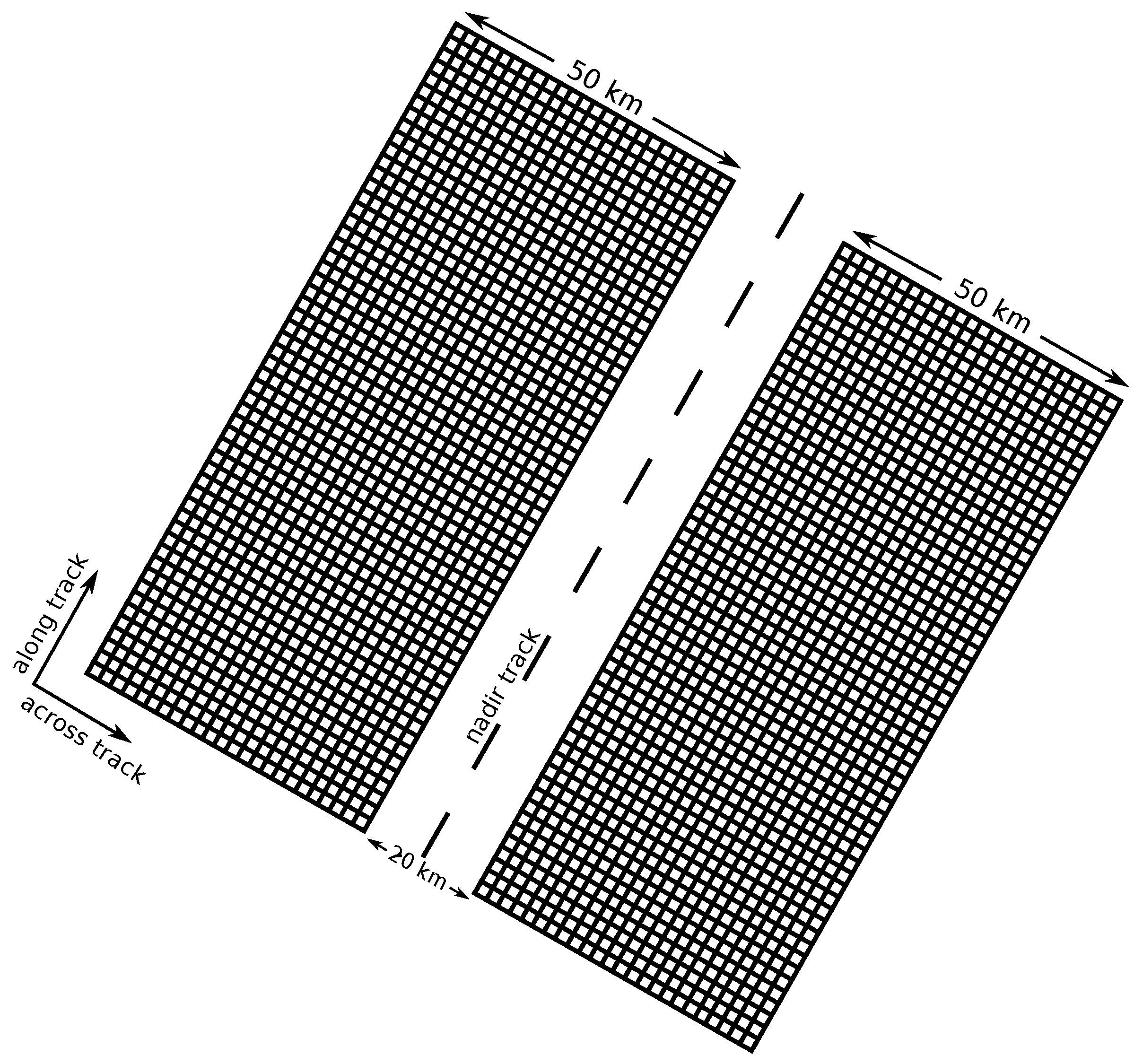
2.1. Synthetic SWOT Data

2.1.1. Synthetic SWOT Data Creation

The present study is conducted on an observing system simulation experiment (OSSE) which considers a high resolution model simulation to be the true state of the ocean. The simulation has been carried out with the NATL60 (North Atlantic, 1/60° resolution) configuration of the NEMO (Nucleus for European Modelling of the Ocean) modelling system [14], version 3.5. The horizontal resolution of 1/60° corresponds to 0.8 to 1.6 km, depending on latitude, while the vertical grid uses 300 levels. With this resolution, we can produce synthetic SWOT data that effectively represent the meso and submesoscale ocean circulation. The NATL60 simulation is the reference simulation in several studies [12,13]. More information on the model set up may be found in NATL60 [19].

The region of study, shown in Figure 1, is the OSMOSIS region in the North Atlantic (44.821°N–55.363°N, 20.016°W–10.008°W; [17]). The OSMOSIS region has very little large scale energy in comparison to the Gulf Stream [17]. This makes OSMOSIS an appropriate region for assessing the SWOT ability to recover small scale dynamics without having large scale structures strongly impact the diagnosis.

Synthetic SWOT data are created from NATL60-simulated SSH fields, using the SWOT simulator for Ocean Science [18,20] developed by the NASA Jet Propulsion Laboratory. In a first step, the SWOT simulator generates a data grid following the predefined swath geometry and orbit ground track. The characteristics of the simulated orbit are detailed in

Table 1. Orbital characteristics of the Science Orbit implemented in the Surface Water and Ocean Topography (SWOT) simulator and used in the present experiments.

Science Orbit
Repeat Cycle (days)	$20.8646$
Repeat Cycle (Orbits)	292
Sub-cycles (days)	$1.10$
Inclination	$77.6$
Elevation (km)	891

.

The SWOT swath is 120 km wide with a 20-km gap in its center (Figure 2).

The spatial resolution is 2 km across and along the track which leads to 50 grid points across track. The grid includes a nadir, along-track line with a resolution of 7 km to simulate the nadir altimeter on-board the SWOT satellite. In a second step, the SWOT simulator interpolates the SSH input fields onto the SWOT grid (wide-swath and nadir). In a third and last step, the simulator randomly generates the main expected SWOT errors, following the specifications of the SWOT error budget document [11]. This is described in more details in the next subsection.

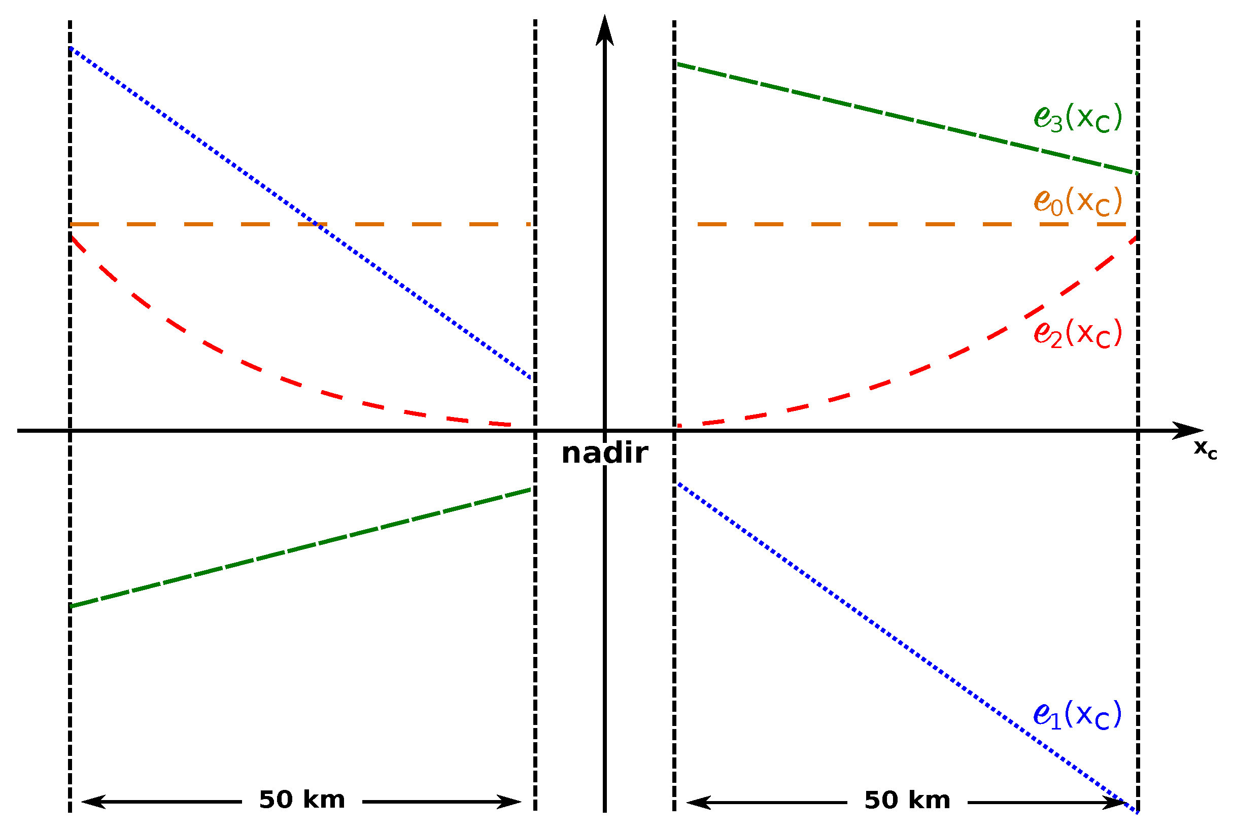
2.1.2. SWOT Data Errors

The SWOT simulator provides statistical models for six components of SWOT measurement errors [11,18]:

• Ka-Band Radar Interferometer (KaRIn) error
• residual roll error
• phase error
• baseline dilatation
• timing error
• wet-troposphere error

The KaRIn instrument random error is a spatially uncorrelated noise with a non-constant variance across track (smiley curve). Several techniques have been developed to specifically de-noise the KaRIn noise impacting the SWOT data [7]. In the present study, we focus on the spatially correlated errors. However, we make the case that because DA is designed to deal with spatially uncorrelated noises, the KaRIn noise is expected to be also reduced by the DA analysis.

The spatially correlated errors have specific across0track structures. Here, we only focus on the across-track structure of the errors, and we consider the error variation for all along track points $x_a$ independently. A discussion on the implications of relaxing this assumption is proposed in Section 4. A schematic representation of the errors cross-track characteristics is presented in Figure 3.

The timing error directly impacts the height measurement and is due to a timing drift in the instrument signal propagation. It also depends on the look angle of the instrument, but at first order, this dependency can be neglected. The timing error $e_0$ is assumed to be constant across track:

$$e_0={\alpha }_0\left(x_a\right)$$

(1)

The roll error is due to the unknown interferometric roll angle and increases linearly across the swath with the distance to the nadir point, i.e., the center of the swath ($x_c=0$). The magnitude of this error can be large. For instance, a tilt of $1/10,000°$ generates a 6-cm error at a point 35 km away from the nadir point. The roll error is considered linear across track:

$$e_1={\alpha }_1\left(x_a\right)x_c$$

(2)

where $e_1$ is the across track roll error, proportional to the cross-track coordinate $x_c$.

When the baseline of the satellite dilates, the length of the baseline varies and modifies the height measurements. This variation creates a deviation for the calibrated instrument signals at each end of the mast. The baseline dilatation error $e_2$ is a quadratic function of the cross-track coordinate:

$$e_2={\alpha }_2\left(x_a\right)x_c^2$$

(3)

The SWOT interferometric instrument combines signals from two sensors which can have relative phase variations between one another. These variations produce a phase drift which translates into a cross-track linear error, independent in each half-swath. The phase error can thus be written as follows:

$$e_3=[{\alpha }_3\left(x_a\right)+{\alpha }_4\left(x_a\right)x_c]\mathcal{H}(-x_c)+[{\alpha }_5\left(x_a\right)+{\alpha }_6\left(x_a\right)x_c]\mathcal{H}\left(x_c\right)$$

(4)

where $\mathcal{H}\left(x\right)$ is the Heaviside function which equals 1 when $x>0$ is true and is 0 otherwise.

Finally, the variability of the water vapor content in the troposphere is a well-known source of error in satellite observations of the ocean also known as the wet-troposphere error (e.g., the missions AMSR-E [21], Jason 1 [22], and Jason 2 [23]). The wet-tropospheric path delay introduces isotropic error correlations. However, what we call the wet-troposphere error throughout the present paper is the residual path delay after a correction performed by a 2-beam radiometer. Since this error is not structured like the four others described previously, we do not intend to reduce it with the error reduction method described below.

Under the previous assumptions on the various errors impacting the SWOT data, it is possible to infer the cross-track structure of the total error:

$$e_{\mathrm{total}}={\alpha }_0+{\alpha }_1{x}_c+{\alpha }_2{x}_c^2+[{\alpha }_3+{\alpha }_4{x}_c]\mathcal{H}(-x_c)+[{\alpha }_5+{\alpha }_6{x}_c]\mathcal{H}\left(x_c\right)$$

(5)

where the explicit dependence of ${\alpha }_i$, for $i=0,\dots ,6$, on $x_a$ has been dropped for the sake of clarity. Knowing the structure of the total error across track is an important information that can be used to understand the strong impact of the spatial error correlations on the SWOT signal and to hopefully reduce some of this impact.

2.2. The Error Reduction Method

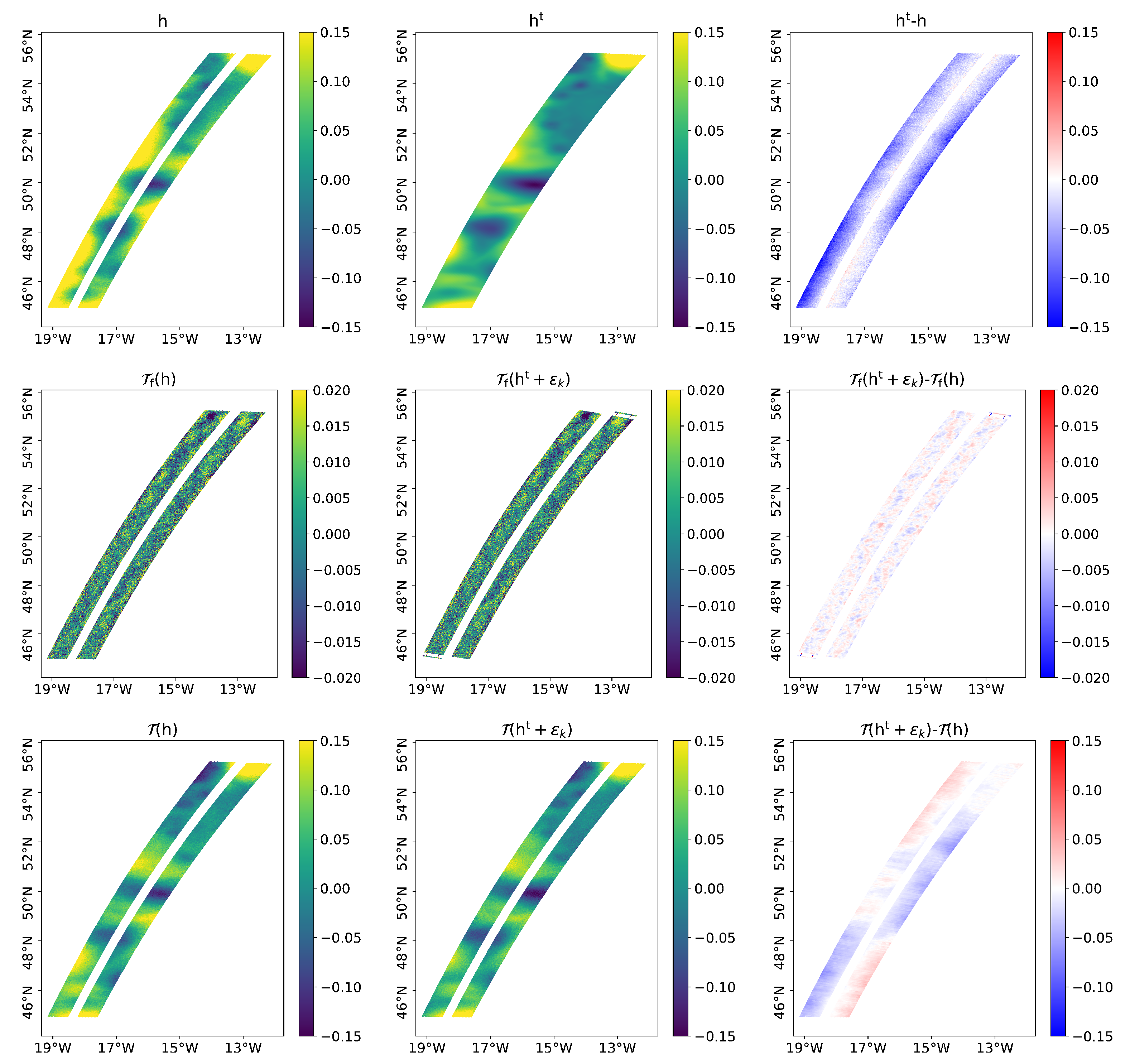
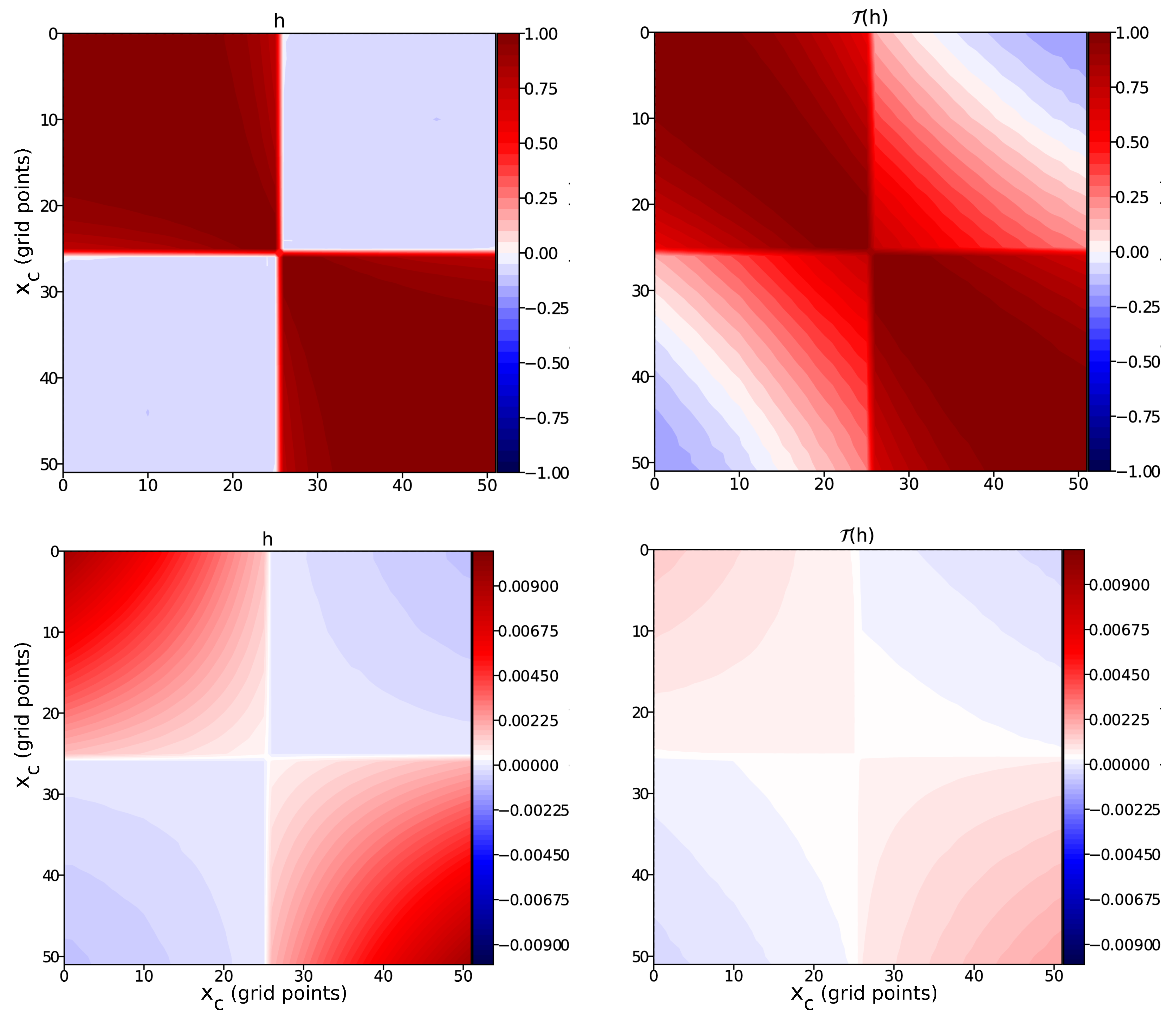
2.2.1. SWOT Data Detrending

To reduce the cross-track spatially structured errors described in the previous section, we first propose to project the SWOT signal h in a nonphysical space spanned by the spatially structured errors. Then, the detrending consists in substracting the projected signal from the across track SWOT signal. The projection coefficients are calculated by minimizing the cost function:

$$\mathcal{J}\left(\alpha \right)={\displaystyle \sum _{x_c=-\frac{n_c}{2}}^{\frac{n_c}{2}}}{\left(h(x_c,x_a)-\{{\alpha }_0+{\alpha }_1{x}_c+{\alpha }_2{x}_c^2+[{\alpha }_3+{\alpha }_4{x}_c]\mathcal{H}(-x_c)+[{\alpha }_5+{\alpha }_6{x}_c]\mathcal{H}\left(x_c\right)\}\right)}^2,$$

(6)

with $n_c$ as the number of across track grid points and with $\alpha =\{{\alpha }_0,{\alpha }_1,{\alpha }_2,{\alpha }_3,{\alpha }_4,{\alpha }_5,{\alpha }_6\}$ as the projection coefficients, functions of $x_a$.

Having calculated the projection coefficients, the straightforward detrending uses the projection of the SSH $h(x_c,x_a)$ for each along track point $x_a$:

$${\mathcal{T}}_f\left(h(x_c,x_a)\right)=h(x_c,x_a)-\{{\alpha }_0+{\alpha }_1{x}_c+{\alpha }_2{x}_c^2+[{\alpha }_3+{\alpha }_4{x}_c]\mathcal{H}(-x_c)+[{\alpha }_5+{\alpha }_6{x}_c]\mathcal{H}\left(x_c\right)\}.$$

(7)

Figure 4 (second row-left panel) shows the full detrending ${\mathcal{T}}_f\left(h\right)$ applied to the SWOT observation h (first row-left panel) corresponding to the true ocean state $h^{\mathrm{t}}$ (first row-right panel) on pass “p031” of cycle 17 in the OSMOSIS region.

When comparing the full detrending of the SWOT data to the full detrending of the true signal plus the KaRIn error only (second row-center) and when looking at the difference between the two (second row-right), we can see that the errors are almost entirely removed. However, the full detrending also removes a large part of the large-scale SSH signal. To limit this effect, we propose a detrending constant along track $\mathcal{T}\left(h\right)$ based on the previously computed coefficients averaged over the entire pass:

$$\mathcal{T}\left(h(x_c,x_a)\right)=h(x_c,x_a)-\{\widetilde{{\alpha }_1}{x}_c+\widetilde{{\alpha }_2}{x}_c^2+[\widetilde{{\alpha }_3}+\widetilde{{\alpha }_4}{x}_c]\mathcal{H}(-x_c)+[\widetilde{{\alpha }_5}+\widetilde{{\alpha }_6}{x}_c]\mathcal{H}\left(x_c\right)\},$$

(8)

for all $x_a$ and all $x_c$, where $\widetilde{{\alpha }_i}$ for $i=1,\dots ,7$ are the along track average of the projection coefficients ${\alpha }_i$ computed in Equation (6). The rationale for this choice is the assumption that the coefficients ${\alpha }_i$ for $i\ne 0$ vary along the track with much larger scales than the oceanic features observed by SWOT. In our setup, we further assumed that the SWOT passes are small enough to consider these coefficients constant along-track. For longer passes, such an assumption would not hold anymore and a more sophisticated approach should be considered. The slow-variation assumption does not hold for the timing error ${\alpha }_0$. This term is therefore removed from the detrending, Equation (8), which implicitly means that this error remains in the detrended SWOT data. The resulting detrended SWOT data $\mathcal{T}\left(h\right)$ for pass “p003” at cycle 17 is shown in the third row-left panel of Figure 4. A large part of the SSH signal is preserved by the detrending, yet the large scale errors shown in the difference $h^{\mathrm{t}}-h$ (first row-right) are reduced.

Figure 5 shows the across-track correlation (top) and covariance (bottom) matrices for the SWOT data h (left) and the detrended SWOT data (right). The error covariances (and the variances in particular) are still present but well-reduced by the detrending. The error correlation matrix after detrending is slightly closer to a diagonal matrix, i.e., the errors are less correlated across the track. Finally, the error correlation matrix after detrending is closer to a Gaussian correlation above and below the diagonal. Note that this form of correlation matrix is typical of the wet-troposphere error not taken into account by the detrending.

It is crucial to note that a significant part of the large scale signal has been removed in the detrended SWOT data and can thus not be considered as SSH information. Hence, we need to find a way to correct an actual SSH variable by using the information contained in the detrended SWOT data. Here, we argue that an appropriate way to address this question comes from data assimilation techniques.

2.2.2. Reducing Errors Using Data Assimilation

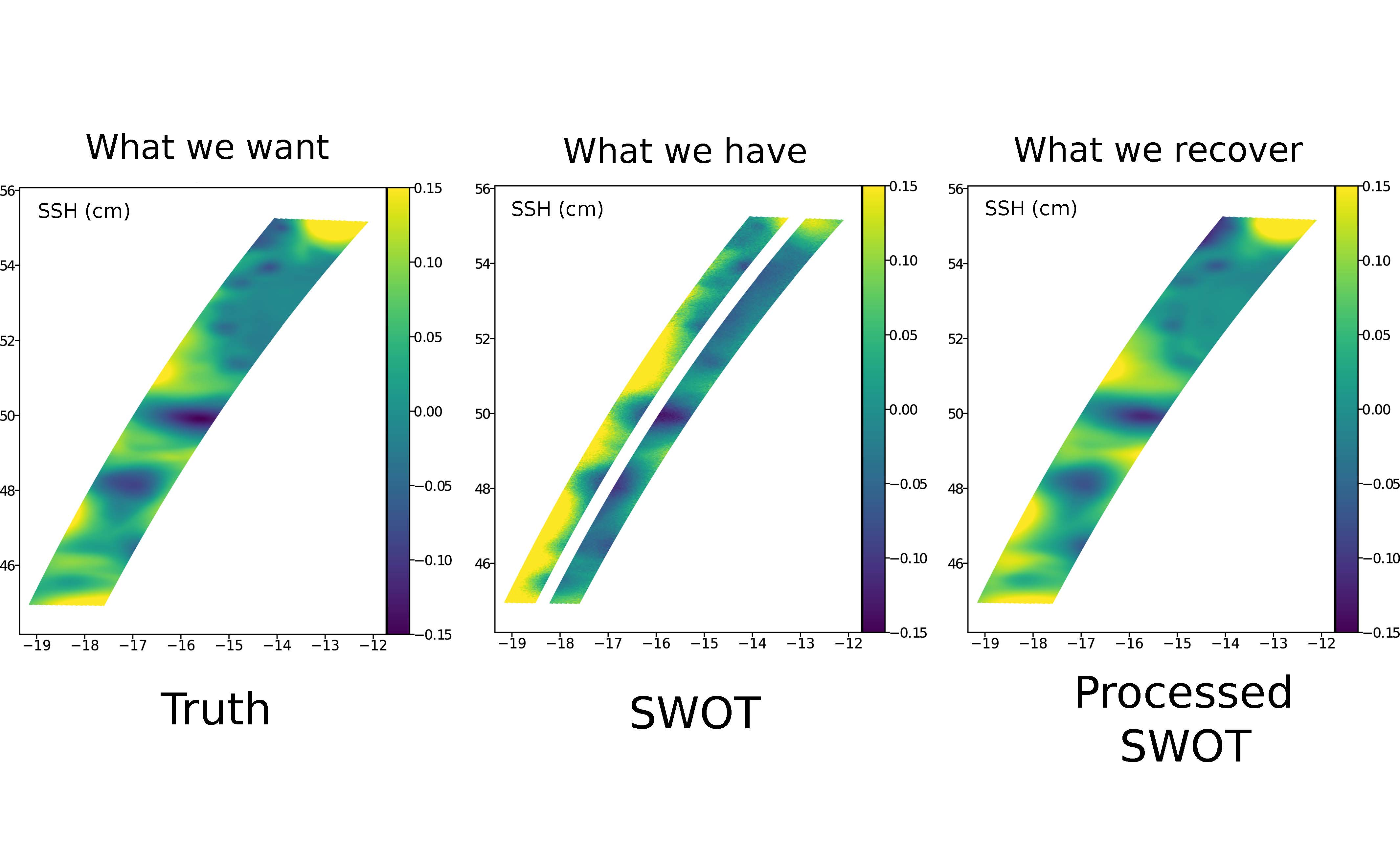
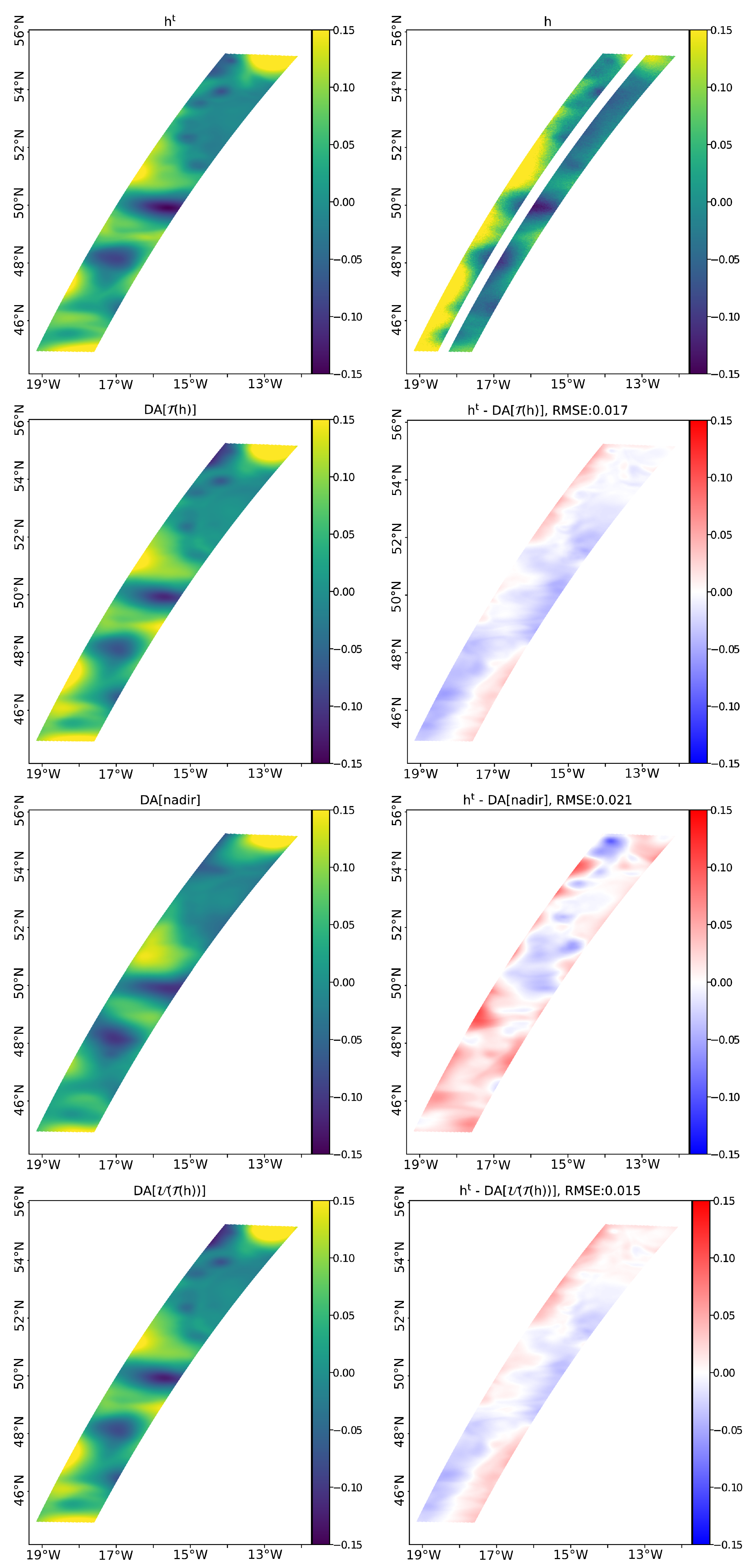
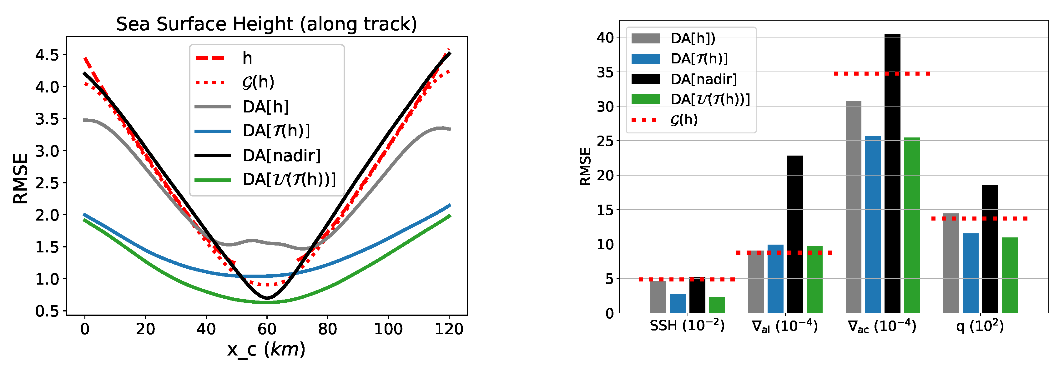
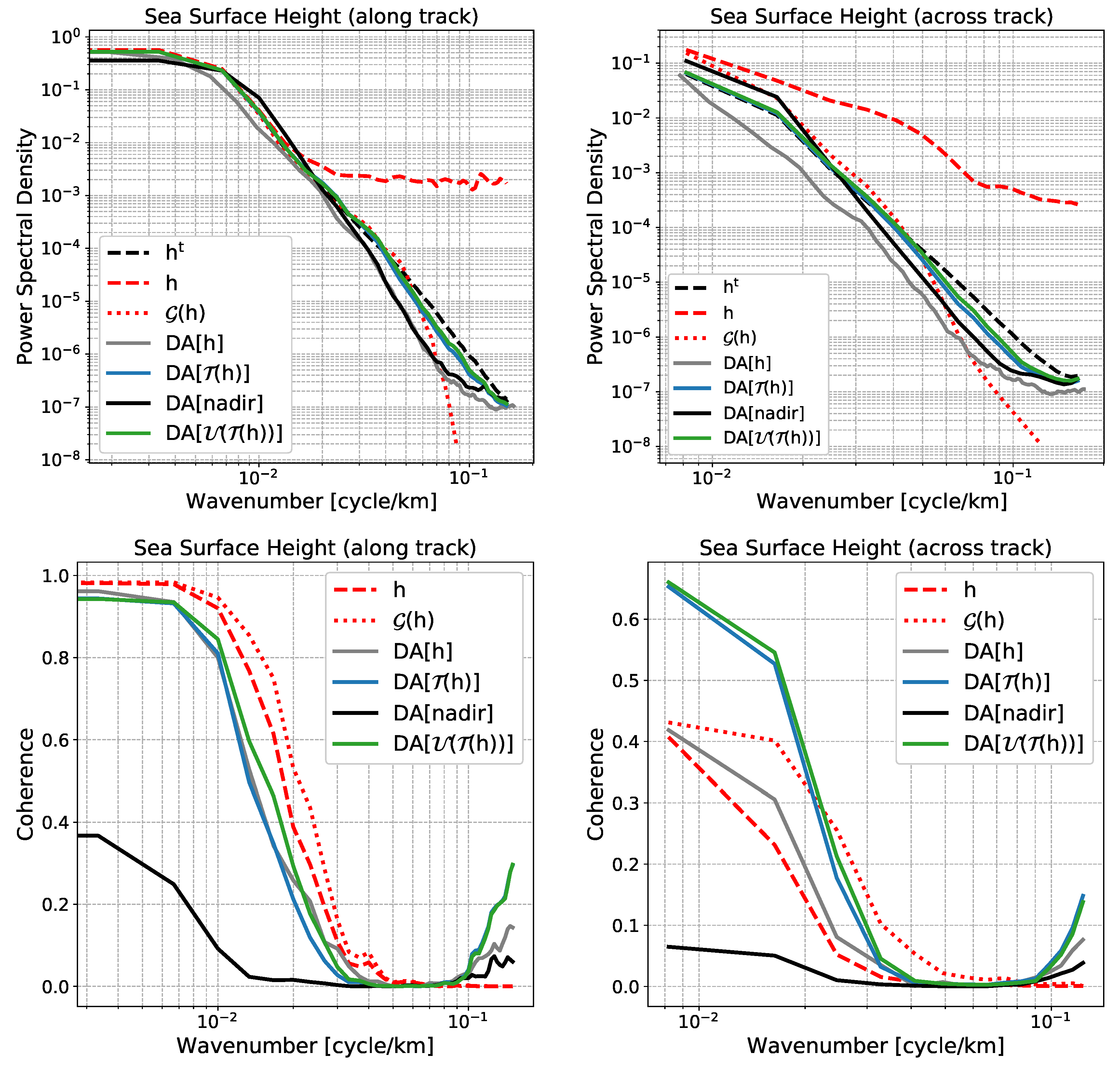
Data assimilation (DA) is a mathematical and methodological approach that allows the combination of different sources of information on a system and the uncertainties that surrounds them in order to recover an updated, more accurate knowledge of that system. The development and the application of DA in geosciences is a large and well-settled field of investigation (e.g., [24,25,26,27,28]) and, in particular, in oceanographic applications [29,30,31,32,33]. The main focus of DA so far has been state and parameter estimation. In the present paper, we propose to use DA to estimate the true SSH SWOT signal from the detrended SWOT data and constrained by high resolution SSH scenes.

The two sources of information that we use in this error reduction method are, on the one hand, the detrended SWOT data (the observation) and, on the other hand, a high-resolution ensemble of unrelated (to the truth) SSH fields (the prior). The ensemble of SSH fields is previously interpolated on the SWOT swath. An ensemble-based DA analysis (e.g., an ensemble Kalman filter (EnKF); see Appendix B) can then be performed in the “SWOT-space”, i.e., finding a more accurate SWOT estimate from an ensemble of prior SWOT-like data and the detrended SWOT data.

Note that we do not directly replace the SWOT data by the detrended SWOT data in the SSH state space, which would be mathematically incorrect; we rather perform the assimilation in the nonphysical detrended space. In practice, this means that an observation operator is created to link the variations of the prior ensemble and the variations of the SWOT data in the detrended space and uses that information to correct an actual SSH. In other words, this error reduction method can be seen as an optimal interpolation scheme [24] as in Section 2.2 but with a prior error covariance matrix given by high-resolution SSH scenes.

It is also possible to apply the same method but to use different observations instead of using the detrended SWOT data. For instance, in the numerical experiments below, this is done using successively the original SWOT data, the nadir data and the nadir-adjusted detrended SWOT data (defined in Section 3.3). Since most DA schemes make the assumption of uncorrelated observation errors and since the detrending reduces the SWOT error correlations, we expect that an assimilation of the detrended SWOT data $\mathcal{T}$ defined by Equation (8) will be much more efficient than the straightforward SWOT data assimilation.

3. Results

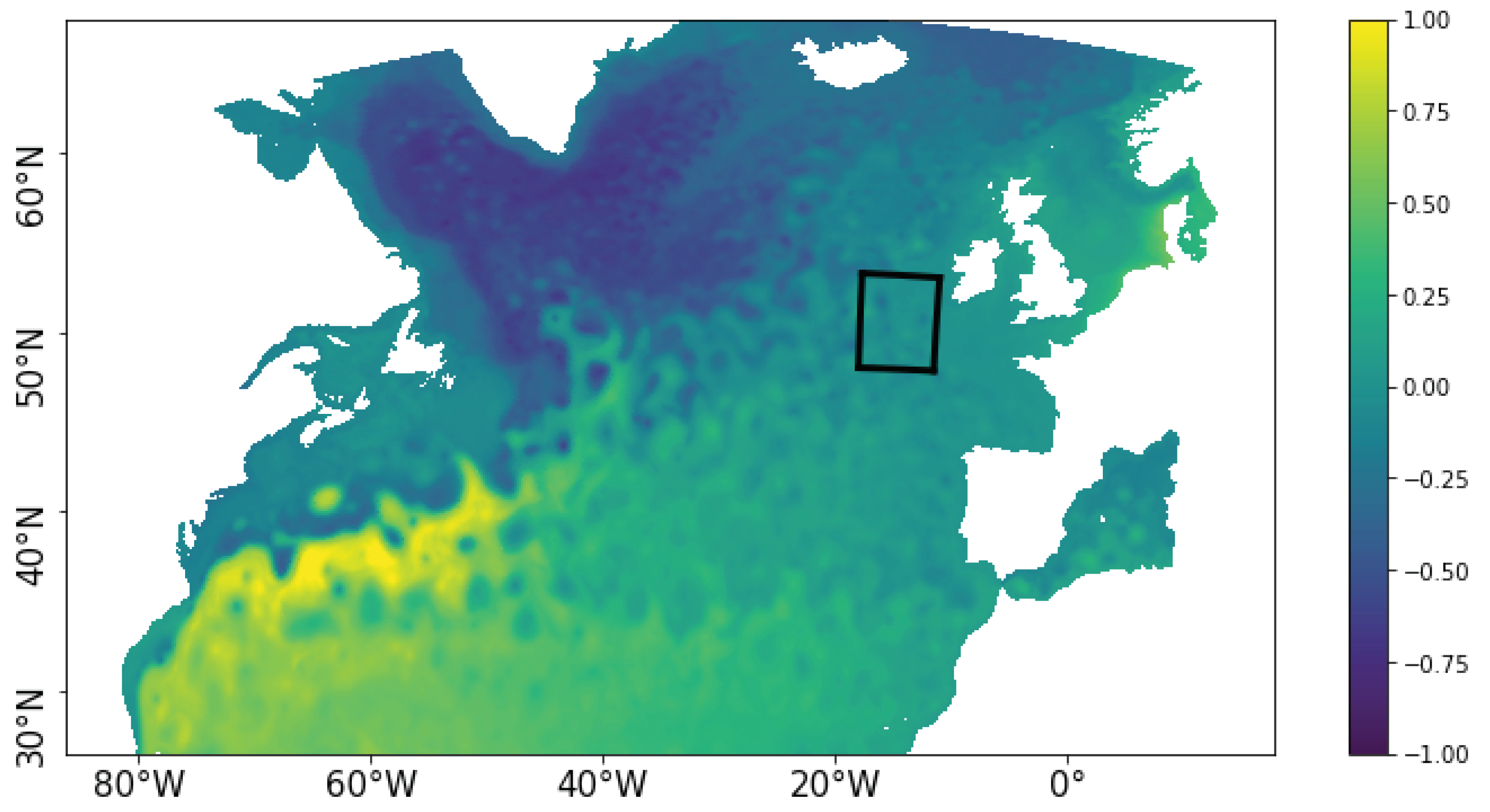
3.1. The Experimental Setup

The synthetic SWOT data are generated from hourly outputs of the NATL60 simulation between 1 October 2012 and 30 September 2013. The OSMOSIS region, as considered in this study, is visited by 28 passes per satellite cycle, with a total of 18 cycles over the year. The numerical experiments are carried out for the first three passes (“p003”, “p031”, and “p059”) of all 18 cycles, which amounts to a total of 54 SWOT datasets.

The error reduction method described in Section 2.2.2 is performed with an EnKF analysis (Appendix B), using a static ensemble made of 60 SSH fields randomly picked in the simulation between 16 June 2012 and 31 August 2012. The static ensemble is randomly picked from a different time period than the experiment in order to avoid consanguinity between the ensemble and the artificial observations. The specific DA parameters are detailed in Appendix C.

Comparisons are performed between the true state of the ocean in the swath, which would correspond to an error free SWOT observation, and the SWOT estimations: the original SWOT data (from the SWOT simulator), the SWOT data filtered with a Gaussian filter, the results of DA using the SWOT data, the detrended SWOT data, the SWOT nadir, and the detrended SWOT data adjusted by the nadir (this adjustment is described in Section 3.3). See

Table 2. A glossary of the variable names and markers for the experimental results.

Notations and Markers
Truth	$h^{\mathrm{t}}$	Dashed black line
SWOT observation	h	Dashed red line
Gaussian filtered SWOT	$\mathcal{G}\left(h\right)$	Dotted red line
SWOT DA	$\mathrm{DA}\left[h\right]$	Grey
Detrended SWOT DA	$\mathrm{DA}\left[\mathcal{T}\right(h\left)\right]$	Blue
Nadir DA	$\mathrm{DA}\left[\mathrm{nadir}\right]$	Orange
Nadir-adjusted detrended SWOT DA	$\mathrm{DA}\left[\mathcal{U}\right(\mathcal{T}\left(h\right)\left)\right]$	Green

for a glossary of the compared variables.

The Gaussian filter is applied to the original SWOT data that has been inpainted using a bivariate spline approximation in order to close the gap. The Gaussian filter is used with a 6-km standard deviation and has a smoothing effect that reduces the very small scale errors, in particular the KaRIn errors. Hence, in addition to the original SWOT data, the comparison to the SWOT data filtered with a Gaussian filter allows to only assess the error reduction method on the large scales.

The error reduction methods are illustrated with a focus on one specific pass and are assessed using the 54 SWOT scenes with root-mean-square errors (RMSE) and spectral diagnostics. RMSE scores on SSH are computed by cross-track coordinate and globally. Global RMSEs are also computed for SSH gradients and Laplacian (relative vorticity). Spectral diagnostics include along and across-track power spectrum densities and spectral coherences.

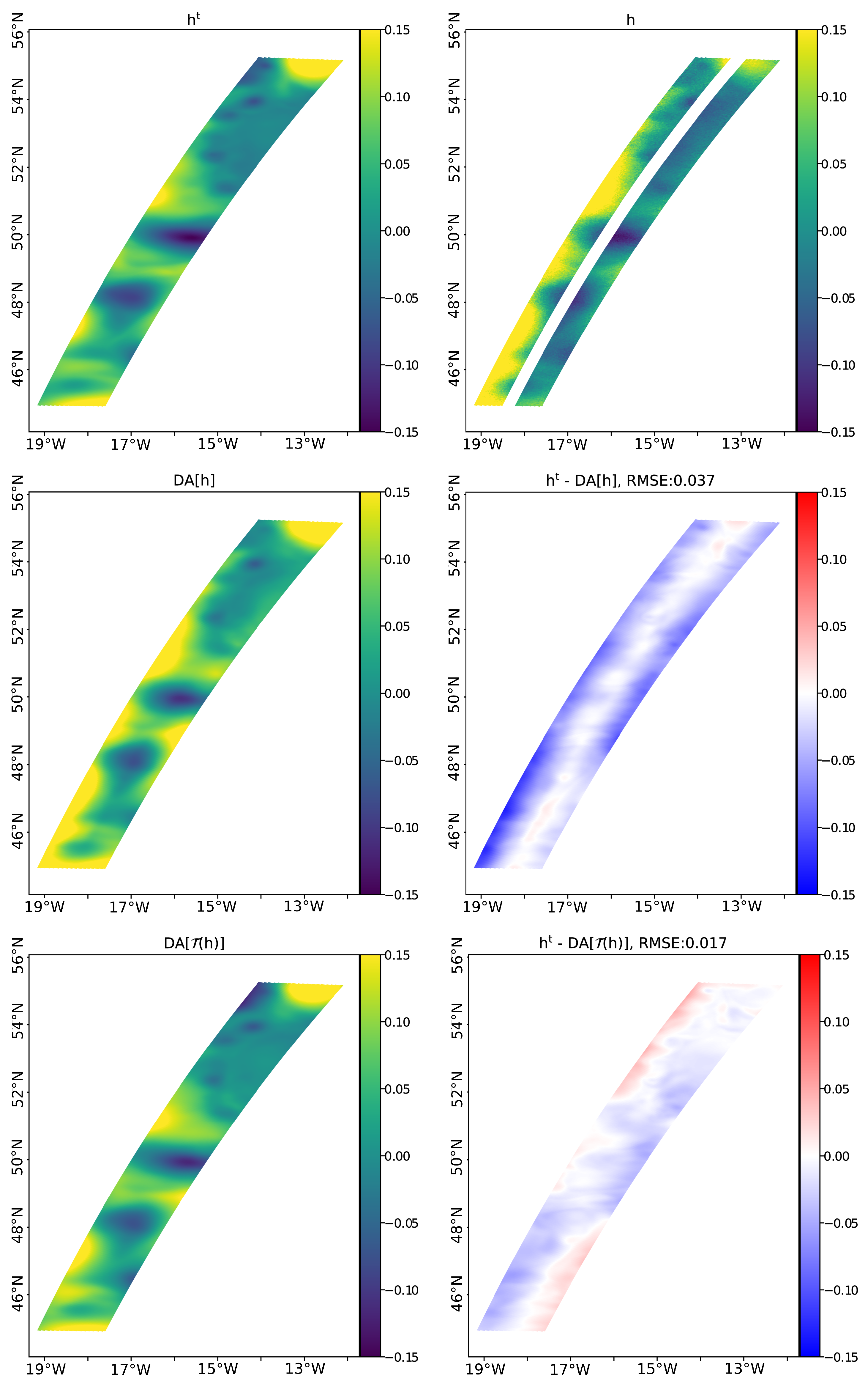
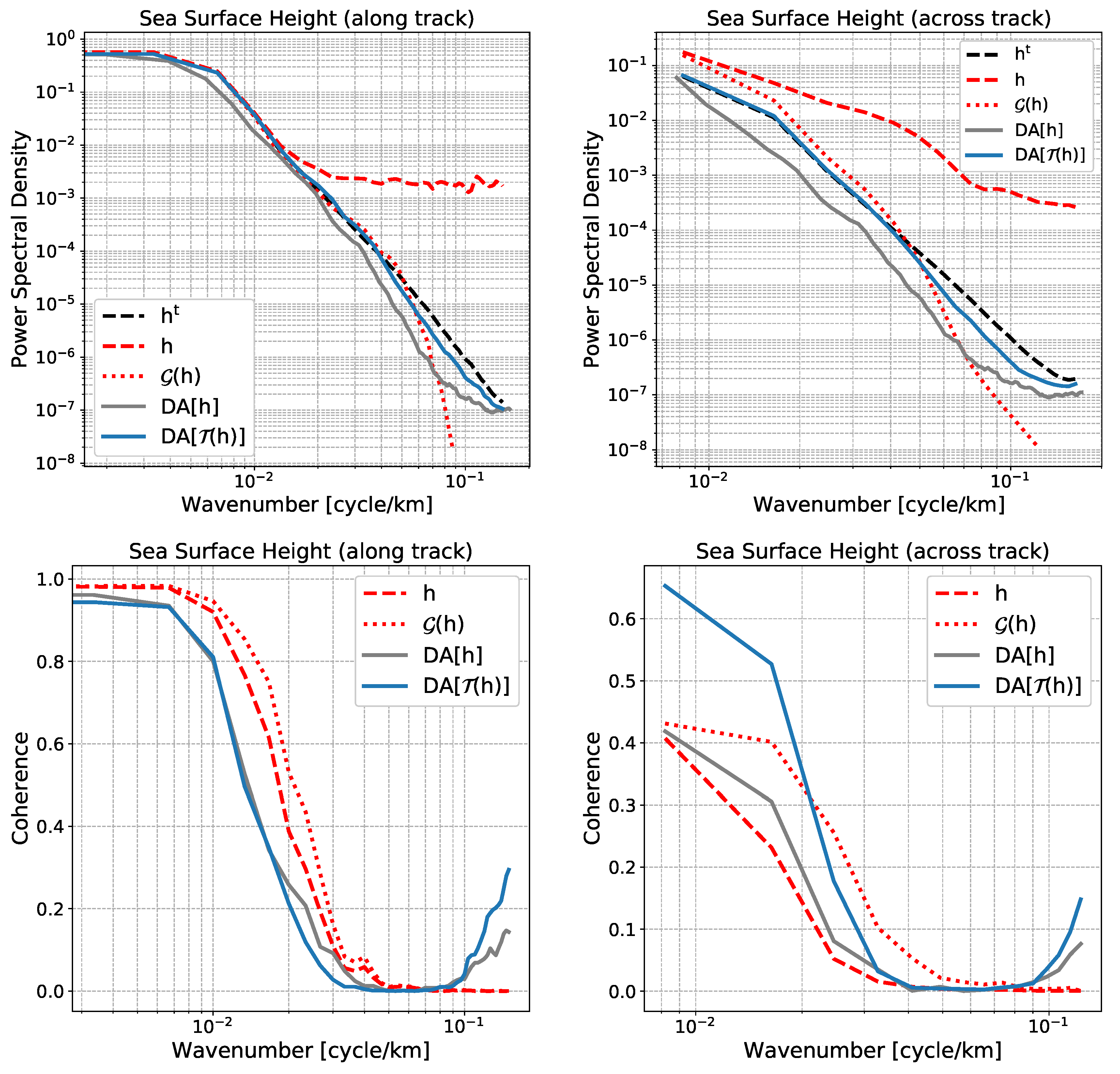
3.2. Error Reduction by Assimilating Detrended SWOT Data

Figure 6 displays an illustration on “p031” at cycle 17 of the error reduction method assimilating the original SWOT data (DA[h]) and the detrended SWOT data (DA[$\mathcal{T}\left(h\right)$]). The two top-row panels, showing the truth $h^{\mathrm{t}}$ and the SWOT data h are identical to those in Figure 4. The second and third rows show the results of the error reduction method (DA[h] and DA[$\mathcal{T}\left(h\right)$] respectively), on the left panels and the point-wise differences of those results to the truth ($h^{\mathrm{t}}$-DA[h] and $h^{\mathrm{t}}$-DA[$\mathcal{T}\left(h\right)$] respectively) on the right panels. Using the detrended SWOT data rather than SWOT in the error reduction method shows a clear improvement. The RMSE, for this pass, gives an accuracy increase of more than 50%.

The two error reduction methods are applied to the 54 SWOT passes. Figure 7 shows the along-track RMSE (left panel) and the global RMSE on SSH, along and across-track gradients, and relative vorticity (right panel). As expected, the SWOT cross-track errors on SSH (red dashed line) are larger close to the outside edges of the double-swath. Applying a Gaussian filter to SWOT ($\mathcal{G}\left(h\right)$, red dotted line) does not reduce these strong cross-track errors. An assimilation of the the raw SWOT data (grey line) reduces marginally the errors close to the edges of the swath and does not recover well the gap between the half-swathes. The cross-track error reduction of the detrended SWOT DA is more substantial, especially close to the edges of the swath. It must be noted though that the inpainting combined with Gaussian filtering shows a better error reduction at the very center of the gap. Following the global RMSE diagnostics (Figure 7, right panel), the improvement by the detrended SWOT DA is confirmed on the SSH, the across-track gradient ${\nabla }_{\mathrm{ac}}$, and the relative vorticity q. Notably, the good RMSE reduction on SSH is confirmed over all passes with an approximately 50% reduction. The RMSE of DA[$\mathcal{T}\left(h\right)$] slightly increases on the along-track gradient. Indeed, the assimilation of the detrended SWOT data may have a slight smoothing effect, which can degrade the gradients. Since the error reduction method does not correct much in the along-track direction, this smoothing effect becomes visible.

Spectral diagnostics have also been performed. Figure 8 (top panels) shows the SSH power spectral density computed along (left) and across (right) the track. Both the Gaussian filtered SWOT data and the detrended SWOT DA recover the true $h^{\mathrm{t}}$ along-track spectral density (dashed black line) down to 25 km scales. The across-track spectral densities of SWOT, Gaussian filtered SWOT data, and DA[h] are over energetic in the large scales (over 100 km scales). When using the detrended SWOT data, the error reduction method manages to estimate the correct energy throughout the spectra down to 25 km scales. In terms of spectral coherence (Figure 8, bottom panels), the estimations are degraded under the 50 km scales. Once again, the assimilation tends to smooth some structures and results in no spectral coherence improvement under 50 km scales and a slight spectral coherence degradation at all scales in the along-track direction. Nonetheless, a large across track spectral coherence improvement is made in the large scales.

3.3. Combining Nadir and SWOT Data

In this experiment, we assess the improvements that can be obtained by the introduction of another source of information: the SWOT nadir data.

As mentioned in Section 2.2.1, the SWOT data detrending $\mathcal{T}$ defined in Equation (8) does not take into account the constant term $\widetilde{{\alpha }_0}$. This constant term was omitted in order to avoid removing a nonzero SSH signal average. Here, we use the nadir information in order to remove the error-generated nonzero SWOT average while preserving the SSH signal average. In practice, we compute the nadir-adjusted detrending as follows:

$$\mathcal{U}\left(\mathcal{T}\left(h\right)\right)=\mathcal{T}\left(h\right)-w·(\overline{\mathcal{T}\left(h\right)}-\overline{\mathrm{nadir}})$$

(9)

where $\overline{\mathcal{T}\left(h\right)}$ and $\overline{\mathrm{nadir}}$ are, respectively, the detrended SWOT data average and the nadir data average (over the pass) and where w is a prescribed weight (hereunder, $w=0.6$) representing the SWOT/nadir error ratio. The error reduction method based on the nadir-adjusted detrended SWOT data is denoted DA[$\mathcal{U}\left(\mathcal{T}\right(h\left)\right)$]. We also implemented the error reduction method using the nadir data only: DA[nadir]. Other experiments (not shown here) have been performed by assimilating simultaneously the detrended SWOT data and the nadir data, but the assimilation of the nadir degraded the performances, especially at the small scales.

Figure 9 shows the illustration pass “p003” at cycle 17, introduced in Figure 6, comparing two additional results: DA[nadir] and DA[$\mathcal{U}\left(\mathcal{T}\right(h)$]. The illustration seems to suggest that the error reduction method using the nadir data only partly recovers the large scale errors but fails to capture the smaller scales. Meanwhile, combining the nadir data with the detrended SWOT data, i.e., DA[$\mathcal{U}\left(\mathcal{T}\right(h\left)\right)$] versus DA[$\mathcal{T}\left(h\right)$], improves the error reduction. This result is confirmed in Figure 10 which, similar to Figure 7, shows the along-track (left) and global (right) RMSE assessing the two additional results. Interestingly, the DA[nadir] errors plotted across-track are very close to the SWOT errors. This across-track shape of the DA[nadir] errors is due to the localization technique used in the assimilation scheme: The SSH corrections due to the assimilation fade out with the distance to the nadir. At the center of the track ($x_c=60$ km), the nadir data are accurate (only nadir altimeter error and troposphere error) and the assimilation analysis manages to recover information left and right of the nadir.

The main result here is that combining nadir and SWOT by adjusting the detrended SWOT data with the nadir helps reduce SSH RMSE. In particular, there is a gain in accuracy at the center of the track where the estimate of the error reduction method is now more accurate than the Gaussian filtered SWOT data $\mathcal{G}\left(h\right)$. This gain appears as well in the global SSH RMSE.

Finally, the spectral analysis in Figure 11 confirms the poor capability of a nadir (alone) assimilation to recover a two-dimensional signal. However, the use of the nadir to adjust the detrended SWOT data for the error reduction method DA[$\mathcal{U}\left(\mathcal{T}\right(h\left)\right)$] slightly improves the power spectral densities and the spectral coherences.

4. Discussion

The data from the future SWOT, wide-swath ocean altimetry mission are expected to be impacted by large, spatially structured and correlated errors. If we want to reach the degree of accuracy and resolution made theoretically achievable by the SWOT system configuration, we need to reduce these errors and their correlations.

Based on the current knowledge of the expected SWOT errors and their cross-track structure, we propose an error reduction method to remove the part of the SWOT signal that exhibits signatures identical to the structured errors. This results in a new, detrended SSH signal that is not fully physical (since a part of the physical signal might be removed as well) but much less affected by structured errors. In conjunction with the detrending, we also propose a SWOT error reduction method based on a static ensemble data assimilation (DA). Ensemble DA is used to combine the detrended SWOT data information to the information from an independent ensemble of scenarios (e.g., high resolution model fields or reanalysis). The detrended SWOT data are particularly suited to this error reduction method (or more generally to DA) due to the reasonably small spatial correlations in their residual errors. It is indeed common practice in DA to assume the observation errors uncorrelated, and many DA softwares are hard-coded under this assumption. The proposed SWOT detrending can also be incorporated in a fully integrated DA scheme, by convolving it to the existing observation operator: $\mathcal{H}\equiv \mathcal{T}\circ \mathcal{H}$. This should significantly improve the assimilation.

The efficiency of the error reduction method using detrended SWOT data has been assessed with an observing system simulation experiment and by using diagnostics on the physical SSH fields (RMSEs) and their spectral characteristics (power spectra and coherence). This method has been compared to the raw SWOT data, to the Gaussian filtered SWOT data, and to the error reduction method directly using the SWOT data (i.e., without detrending). Most diagnostics show the good performance of the proposed method for the retrieval of SSH on the SWOT swath. Notably, the method recovers the energy of the signal throughout the spectra down to 25 km scales. However, in this work, because the SWOT scenes were not spatially extended, we neglected the along-track variations of the structured errors. However, they may explain the relatively poor results of the error reduction method in the diagnostics based on an along-track processing (RMSE in along-track SSH gradient and along-track spectral coherence). Also, the error reduction method developed in this work addresses the structured errors due to the satellite design but not other errors that may show spatial correlations, e.g., errors due to the atmospheric water vapor. These errors were neglected in this paper, but methods exist to account for them [8,9,34]. The next step should then focus on diagnosing the residual observation error correlations and should check whether it is possible to account for them in the assimilation. Finally, since the performance of ensemble DA partly depends on the quality of the initial ensemble, a natural perspective of the improvement of the method lies in the improvement of the initial ensemble itself. Using seasonally varying ensembles for the timely processing of SWOT data would be a first, easy step. Integrating the detrending procedure in a full DA system would represent the ultimate goal.

The SWOT nadir data can be combined with the error reduction method to improve the accuracy of the SWOT wide-swath estimation. In the last section of the numerical experiments, we introduced the SWOT nadir data in the method. Even though the use of the nadir data has been rather minimalistic, it further improves the error reduction method performance. Yet, with the simple DA configuration used in this exploratory work, the combined assimilation of the nadir data and the detrended SWOT data resulted in destructive interferences (not shown). We did not tackle this technical DA issue here to not deviate from our primary focus, the wide-swath data. However, it will have to be done if the error reduction method is selected for operational applications in the future.

Although the experiments presented in this paper are based on an advanced observing system simulation experiment, further validations before operational applications are required. It should be noted that the experiments presented in this study are based on synthetic SWOT observations from a state-of-the-art high resolution submesoscale permitting ocean model simulation (NEMO-NATL60). However, this model simulation does not account for the high frequency internal tides that will affect SWOT SSH signals at scales <100 km [15,16]. It is unclear how the efficiency of the method presented in this study would be affected by the representation of high frequency internal tides in the model. We are optimistic because the horizontal scales of the internal tide signal and of the correlated SWOT error in the along-track direction (as anticipated by the SWOT project team) differ by an order of magnitude (100 km vs 1000 km, respectively). The along-track averaging performed in the detrending process should therefore be rather insensitive to the internal tide signal, providing it exhibits some sort of periodicity, but this is highly speculative. To properly evaluate the method performance in presence of internal tide signal, experiments must be carried out with appropriate numerical simulations. This will be done in future studies.

5. Conclusions

The present paper is a proof-of-concept for the future SWOT data pre-processing, showing that an error reduction method based on the detrending of the spatially structured errors and the retrieval of the large-scale physical signal with ensemble data assimilation can help recover a large part of the SWOT SSH signal. Notably, the detrending step of the method is an innovation in itself that can be separately incorporated in an operational data assimilation scheme and can enhance its performance. This paper should therefore be seen as a first demonstration for a method that can be further improved and could ultimately be used operationally. The method leads to accurate estimations of the SSH signal and allows for the retrieval of spectral energy down to the 25 km scales.

Further developments are needed in order to improve the method and to reduce the errors at finer scales. The first step of the method, the detrending, could be improved by accounting for the along-track variations of the structured errors with, for instance, an along-track processing of the detrending coefficients. Also, the two-dimensional structured errors, such as the wet-troposphere errors, are not taken into account in the detrending process. Hence, a two-dimensional detrending or a combination of the current cross-track detrending and other existing methods [8,9,34] should be investigated. The second step of the method, the retrieval, could be improved by using a larger and/or a more appropriate ensemble of SSH scenes, for instance, a seasonally-varying ensemble. A craftier methodology for combining the two-dimensional SWOT data with the SWOT nadir data should also be studied. Finally, in order to further strengthen the validation of the method, an assessment of its capacity to recover the SSH SWOT signal in an experimental setup that includes high frequency internal tides should be performed.

The primary oceanographic objective of the SWOT mission is to observe the ocean circulation determined from the ocean surface topography at spatial resolutions of 15 km for 68% of the ocean [35]. Two major challenges before reaching this goal are (i) the assimilation of the data at their nominal, 2-km resolution (pixel size), where the amplitude of the correlated errors are comparable to the signal, and (ii) the separation of the signals from the balanced dynamics, internal tides, and noise. Although further investigations are needed regarding the internal tides, the method proposed here will contribute to addressing both challenges and, hopefully, will make the SWOT mission approach its main scientific objective.

References

1. Durand, M.; Fu, L.L.; Lettenmaier, D.; Alsdorf, D.; Rodriguez, E.; Esteban-Fernandez, D. The Surface Water and Ocean Topography Mission: Observing terrestrial surface water and oceanic submesoscale eddies. Proc. IEEE 2010, 98, 766–779. [Google Scholar] [CrossRef]
2. Fu, L.L.; Ferrari, R. Observing oceanic submesoscale processes from space. Eos Trans. Am. Geophys. Union 2008, 89, 488. [Google Scholar] [CrossRef]
3. Fu, L.L.; Alsdorf, D.; Rodriguez, E.; Morrow, R.; Mognard, N.; Lambin, J.; Vaze, P.; Lafon, T. The SWOT (Surface Water and Ocean Topography) Mission: Spaceborne radar interferometry for oceanographic and hydrological applications. In Proceedings of the OCEANOBS’09 Conference, Venice, Italy, 21–25 September 2009. [Google Scholar]
4. McWilliams, J.C. The nature and consequences of oceanic eddies. Ocean Model. Eddy. Regime 2008, 177, 5–15. [Google Scholar]
5. McWilliams, J.C. Submesoscale currents in the ocean. Proc. R. Soc. A Math. Phys. Eng. Sci. 2016, 472, 20160117. [Google Scholar] [CrossRef]
6. Chelton, D.B.; Schlax, M.G.; Samelson, R.M.; Farrar, J.T.; Molemaker, M.J.; McWilliams, J.C.; Gula, J. Prospects for future satellite estimation of small-scale variability of ocean surface velocity and vorticity. Prog. Oceanogr. 2019, 173, 256–350. [Google Scholar] [CrossRef]
7. Gómez-Navarro, L.; Fablet, R.; Mason, E.; Pascual, A.; Mourre, B.; Cosme, E.; Le Sommer, J. SWOT Spatial Scales in the Western Mediterranean Sea Derived from Pseudo-Observations and an Ad Hoc Filtering. Remote Sens. 2018, 10, 599. [Google Scholar] [CrossRef]
8. Ruggiero, G.A.; Cosme, E.J.M.; Le Sommer, J.C. An efficient way to account for observation error correlations in the assimilation of data from the future swot high-resolution altimeter mission. J. Atmos. Ocean. Technol. 2016, 33, 2755–2768. [Google Scholar] [CrossRef]
9. Yaremchuk, M.; D’Addezio, J.M.; Panteleev, G.; Jacobs, G. On the approximation of the inverse error covariances of high-resolution satellite altimetry data. Q. J. R. Meteorol. Soc. 2018, 144, 1995–2000. [Google Scholar] [CrossRef]
10. Dibarboure, G.; Ubelmann, C. Investigating the performance of four empirical cross-calibration methods for the proposed SWOT mission. Remote Sens. 2014, 6, 4831–4869. [Google Scholar] [CrossRef]
11. Esteban-Fernandez, D. SWOT Project Mission Performance and Error Budget Document; JPL Doc. JPL D-79084; NASA: Washington, DC, USA, 2014. [Google Scholar]
12. Fresnay, S.; Ponte, A.L.; Le Gentil, S.; Le Sommer, J. Reconstruction of the 3-D Dynamics From Surface Variables in a High-Resolution Simulation of North Atlantic. J. Geophys. Res. Oceans 2018, 123, 1612–1630. [Google Scholar] [CrossRef] [Green Version]
13. Amores, A.; Jordá, G.; Arsouze, T.; Le Sommer, J. Up to what extent can we characterize ocean eddies using present-day gridded altimetric products? J. Geophys. Res. Oceans 2018, 123, 7220–7236. [Google Scholar] [CrossRef]
14. Madec, G. NEMO ocean engine. In Note du Pôle de Modélisation; No 27; Institut Pierre-Simon Laplace (IPSL): Paris, France, 2015; ISSN 1288-1619. [Google Scholar]
15. Qiu, B.; Chen, S.; Klein, P.; Wang, J.; Torres, H.; Fu, L.L.; Menemenlis, D. Seasonality in transition scale from balanced to unbalanced motions in the world ocean. J. Phys. Oceanogr. 2018, 48, 591–605. [Google Scholar] [CrossRef]
16. Gula, J.; Blacic, T.M.; Todd, R.E. Submesoscale coherent vortices in the Gulf Stream. Geophys. Res. Lett. 2019, 46. [Google Scholar] [CrossRef]
17. Buckingham, C.E.; Naveira Garabato, A.C.; Thompson, A.F.; Brannigan, L.; Lazar, A.; Marshall, D.P.; George Nurser, A.J.; Damerell, G.; Heywood, K.J.; Belcher, S.E.; et al. Seasonality of submesoscale flows in the ocean surface boundary layer. Geophys. Res. Lett. 2016, 43, 2118–2126. [Google Scholar] [CrossRef] [Green Version]
18. Gaultier, L.; Ubelmann, C.; Fu, L.L. SWOT Simulator Documentation; Tech. Rep. 1.0.0; Jet Propulsion Laboratory, California Institute of Technology: Pasadena, CA, USA, 2015. [Google Scholar]
19. NATL60 Configuration on GitHub. Available online: https://zenodo.org/record/1210116#.XPDnb3GYOUk (accessed on 12 April 2019).
20. SWOT Simulator on GitHub. Available online: https://github.com/SWOTsimulator (accessed on 12 April 2019).
21. Kawanishi, T.; Sezai, T.; Ito, Y.; Imaoka, K.; Takeshima, T.; Ishido, Y.; Shibata, A.; Miura, M.; Inahata, H.; Spencer, R.W. The Advanced Microwave Scanning Radiometer for the Earth Observing System (AMSR-E), NASDA’s contribution to the EOS for global energy and water cycle studies. IEEE Trans. Geosci. Remote Sens. 2003, 41, 184–194. [Google Scholar] [CrossRef]
22. Ménard, Y.; Fu, L.L.; Escudier, P.; Parisot, F.; Perbos, J.; Vincent, P.; Desai, S.; Haines, B.; Kunstmann, G. The Jason-1 mission special issue: Jason-1 calibration/validation. Mar. Geod. 2003, 26, 131–146. [Google Scholar] [CrossRef]
23. Lambin, J.; Morrow, R.; Fu, L.L.; Willis, J.K.; Bonekamp, H.; Lillibridge, J.; Zaouche, G.; Vaze, P.; Bannoura, W.; Parisot, F. The OSTM/Jason-2 mission. Mar. Geod. 2010, 33, 4–25. [Google Scholar] [CrossRef]
24. Daley, R. Atmospheric Data Analysis; Cambridge University Press: Cambridge, UK, 1991. [Google Scholar]
25. Ghil, M.; Malanotte-Rizzoli, P. Data assimilation in meteorology and oceanography. Adv. Geophys. 1991, 33, 141–266. [Google Scholar]
26. Kalnay, E. Atmospheric Modeling, Data Assimilation and Predictability; Cambridge University Press: Cambridge, UK, 2003. [Google Scholar]
27. Asch, M.; Bocquet, M.; Nodet, M. Data Assimilation: Methods, Algorithms, and Applications; Fundamentals of Algorithms, SIAM: Philadelphia, PL, USA, 2016. [Google Scholar]
28. Carrassi, A.; Bocquet, M.; Bertino, L.; Evensen, G. Data assimilation in the geosciences: An overview of methods, issues, and perspectives. WIREs Clim. Chang. 2018, 9, e535. [Google Scholar] [CrossRef]
29. Bennett, A.F. Inverse Methods in Physical Oceanography; Cambridge University Press: Cambridge, UK; New York, NY, USA, 1992. [Google Scholar]
30. Pham, D.T.; Verron, J.; Roubaud, M.C. A singular evolutive extended Kalman filter for data assimilation in oceanography. J. Mar. Syst. 1998, 16, 323–340. [Google Scholar] [CrossRef]
31. Bertino, L.; Evensen, G.; Wackernagel, H. Sequential data assimilation techniques in oceanography. Int. Stat. Rev. 2003, 71, 223–241. [Google Scholar] [CrossRef]
32. Lermusiaux, P.F.J. Uncertainty estimation and prediction for interdisciplinary ocean dynamics. J. Comp. Phys. 2006, 217, 176–199. [Google Scholar] [CrossRef] [Green Version]
33. Sakov, P.; Counillon, F.; Bertino, L.; Lisaeter, K.A.; Oke, P.R.; Korablev, A. Topaz4: An ocean-sea ice data assimilation system for the north atlantic and arctic. Ocean Sci. 2012, 8, 633–656. [Google Scholar] [CrossRef]
34. Brankart, J.M.; Ubelmann, C.; Testut, C.E.; Cosme, E.; Brasseur, P.; Verron, J. Efficient parameterization of the observation error covariance matrix for square root or ensemble Kalman filters: application to ocean altimetry. Mon.Weather Rev. 2009, 137, 1908–1927. [Google Scholar] [CrossRef]
35. Fu, L.L.; Rodriguez, E.; Alsdorf, D.; Morrow, R. The SWOT Mission Science Document; JPL Publication: California, CA, USA, 2012. [Google Scholar]
36. Evensen, G. Data Assimilation: The Ensemble Kalman Filter, 2nd ed.; Springer: Berlin/Heildelberg, Germany, 2009. [Google Scholar]
37. Kalman, R.E. A new approach to linear filtering and prediction problems. J. Basic Eng. 1960, 82, 35–45. [Google Scholar] [CrossRef]
38. Hunt, B.; Kostelicj, E.J.; Szunyogh, I. Efficient data assimilation for spatiotemporal chaos: A local ensemble transform Kalman filter. Physica D 2007, 230, 112–126. [Google Scholar] [CrossRef] [Green Version]
Sample Availability: Samples of the compounds … are available from the authors.
Figure 1. The OSMOSIS region (black box) in an sea surface height (SSH) field (in meters) produced by the NATL60 simulation.
Remotesensing 11 01336 g001
Figure 2. A schematic representation of the SWOT grid at a 2-km resolution.
Remotesensing 11 01336 g002
Figure 3. A schematic representation of the SWOT error distributions across track. The errors e 0 , e 1 , e 2 , and e 3 correspond respectively to the timing, the roll, the baseline dilatation, and the phase errors.
Remotesensing 11 01336 g003
Figure 4. SSH (in meters) on pass “p031” of cycle 17 given by the SWOT data h (first row—left), the true SSH field h t (first row—center), and their difference (first row—right); by the fully detrended (different scale) SWOT data T f ( h ) (second row—left), the fully detrended truth + KaRIn error T f ( h t + ϵ k ) (second row—center), and their difference (second row—right); and by the partially detrended SWOT data T ( h ) (third row—left), the partially detrended truth + KaRIn error T ( h t + ϵ k ) (third row—center), and their difference (third row—right).
Remotesensing 11 01336 g004
Figure 5. The across-track correlations (top) and across-track covariances (bottom) of the SWOT data h (left) and the detrended SWOT data T ( h ) (right).
Remotesensing 11 01336 g005
Figure 6. SSH (in meters) on pass “p031” of cycle 17 given by the truth h t (top-left) and the SWOT data h (top-right) and the results DA[h] (middle-left) and DA[ T ( h ) ] (bottom-left) with their differences to h t (middle-right and bottom-right, respectively).
Remotesensing 11 01336 g006
Figure 7. Left: Along track RMSE over the 54 passes on SSH (10 2 m) of h, G ( h ) , DA[h], and DA[ T ( h ) ] against h t (see Table 2 for notations). Right: Global RMSE on SSH (10 2 m), along and across track gradients al and ac respectively (scaled by 10 4 ) and relative vorticity q (scaled by 10 2 ).
Remotesensing 11 01336 g007
Figure 8. Top: Power spectral density along (left) and across (right) track in the function of spatial frequency (km 1 ) over the 54 passes on SSH of h t , h, G ( h ) , DA[h], and DA[ T ( h ) ] (see Table 2 for notations). Bottom: Same as top but with a spectral coherence against h t .
Remotesensing 11 01336 g008
Figure 9. Same as Figure 6 but compares two additional results: DA[nadir] and DA[ U ( T ( h ) ) ].
Remotesensing 11 01336 g009
Figure 10. Same as Figure 7 but compares two additional results: DA[nadir] and DA[ U ( T ( h ) ) ].
Remotesensing 11 01336 g010
Figure 11. Same as Figure 8 but compares two additional results: DA[nadir] and DA[ U ( T ( h ) ) ].
Remotesensing 11 01336 g011