Tree Species Classification in a Highly Diverse Subtropical Forest Integrating UAV-Based Photogrammetric Point Cloud and Hyperspectral Data

Abstract

The use of remote sensing data for tree species classification in tropical forests is still a challenging task, due to their high floristic and spectral diversity. In this sense, novel sensors on board of unmanned aerial vehicle (UAV) platforms are a rapidly evolving technology that provides new possibilities for tropical tree species mapping. Besides the acquisition of high spatial and spectral resolution images, UAV-hyperspectral cameras operating in frame format enable to produce 3D hyperspectral point clouds. This study investigated the use of UAV-acquired hyperspectral images and UAV-photogrammetric point cloud (PPC) for classification of 12 major tree species in a subtropical forest fragment in Southern Brazil. Different datasets containing hyperspectral visible/near-infrared (VNIR) bands, PPC features, canopy height model (CHM), and other features extracted from hyperspectral data (i.e., texture, vegetation indices-VIs, and minimum noise fraction-MNF) were tested using a support vector machine (SVM) classifier. The results showed that the use of VNIR hyperspectral bands alone reached an overall accuracy (OA) of 57% (Kappa index of 0.53). Adding PPC features to the VNIR hyperspectral bands increased the OA by 11%. The best result was achieved combining VNIR bands, PPC features, CHM, and VIs (OA of 72.4% and Kappa index of 0.70). When only the CHM was added to VNIR bands, the OA increased by 4.2%. Among the hyperspectral features, besides all the VNIR bands and the two VIs (NDVI and PSSR), the first four MNF features and the textural mean of 565 and 679 nm spectral bands were pointed out as more important to discriminate the tree species according to Jeffries–Matusita (JM) distance. The SVM method proved to be a good classifier for the tree species recognition task, even in the presence of a high number of classes and a small dataset.

1. Introduction

Tropical forests are among the most complex ecosystems on Earth, hosting an overwhelming proportion of global tree diversity: approximately 53,000 tree species in contrast to only 124 across temperate Europe [1], they play a crucial role in biodiversity conservation and in ecological dynamics at global scale [2].

According to Viana and Tabanez [3], the Atlantic Rain Forest (Mata Atlântica) is one of the most endangered tropical biomes in the world, as it is reduced to less than 16% of its original area [4]. This biome has been particularly affected by anthropogenic disturbances, such as industrial activities, urbanization, and agricultural expansion, which transformed it in an archipelago of small forest patches embedded into a mosaic of degraded areas, pasture, agriculture, forestry, and urban areas [5]. Currently 1544 plant species [6] and 380 animal species [7] are endangered in this biome, and they represent the equivalent of 60% of the threatened species for both flora and fauna in Brazil [8]. Despite these threats, the Atlantic Rain Forest and its associated ecosystems (sandbanks and mangroves) are still rich in terms of biodiversity, containing high rates of endemism and species diversity, even greater than that observed in the Amazon Forest [9].

Due to the importance of this biome, it is crucial to build a reliable tree species mapping system for several applications, such as resource management, biodiversity assessment, ecosystem services assessment and conservation [10]. In this respect, remote sensing data represents an efficient and potentially economical way of inventorying forest resources and mapping tree species [11,12]. However, so far, few studies focused on tree species classification with remote sensing in tropical forests [13,14,15,16,17,18,19], and, in general, they have been limited to the classification of only three to eight dominant canopy species [14,15,16,17,18,19]. Most of the aforementioned studies reported some common issues that hamper tree species classification in tropical forests, such as high number of species with similar spectral responses, irregularly stratified canopy, overlap between canopies leading to the absence of clear boundaries between individual trees, and the presence of dominant and minority classes, resulting in an imbalanced training data set in which only a small number of samples are available for the less frequently occurring tree species.

Fortunately, some of these problems could be minimized thanks to the improvement of the spatial resolution of the remote sensing sensors in the last decades, which enables the identification of isolated trees even in dense forest canopies. Hyperspectral sensors mounted on manned aircrafts, for instance, could provide data at both high spatial and spectral resolution, being extensively used in tree species classification [14,16,18,20,21,22]. Recently, small-format hyperspectral cameras on-board unmanned aerial vehicles (UAVs) have been on the spotlight and they began to be explored for tree species classification in boreal forests [23,24]. Compared to satellite and airborne data acquisition, UAV-borne methods have many advantages, such as the possibility to collect data even under poor imaging conditions, e.g., under cloud cover, which makes it very operational in a wide range of environmental measuring applications [25]; the cost-efficient data collection with the desired spatial and temporal resolutions; and the nondependence on airports for take-off, or satellite availability in the desired area [26]. As they operate at a lower flight altitude than conventional aerial platforms, they offer a finer spatial resolution [23]. On the other hand, UAVs have limited payload, short flight endurance and they present instability in windy conditions, which restrict their use in small scale applications [27,28].

Spectral UAV sensors can be built using different approaches: point, push broom, or 2D imager [29]. 2D imagers can be classified based on the imaging principle as the ones capturing all bands simultaneously (snapshot imaging), a system that synchronously records spectral bands with several cameras (multicamera), or as those capturing time-sequential bands [29]. Sequential band systems record bands or sets of bands sequentially in time, with a time lag between two consecutive spectral bands. These systems have often been called image frame sensors [25,29].

Besides the high spatial resolution and a considerable number of spectral bands, frame sensors record spectral data in two spatial dimensions within every exposure, opening new ways of imaging spectroscopy [29]. Computer vision algorithms can be used to compose a scene from individual images, and spectral and 3D information can be retrieved from the same data and composed to (hyper)spectral digital surface models [25,30]. Indeed, they allow generation of dense photogrammetric point clouds (PPCs) and digital surface models (DSM), which are not available for conventional hyperspectral instruments based on whiskbroom or push broom scanning [31]. This 3D information can capture differences in vertical structure among species (i.e., tree height, tree patterns, and leaf distributions) [24,31] that can be useful for tree species classification. However, to the best of our knowledge, there is no study on tree species classification using both hyperspectral images and derived PPC features in a tropical forest environment, while few exists in temperate and boreal environments, e.g., Nevalainen et al. [23] and Tuominen et al. [24].

Besides the data, the right choice of the classification method is also decisive for a successful land use and cover mapping [32]. In this respect, the current literature generally recognizes the support vector machine classifier (SVM) for its ability to work well with limited training samples [33], since it utilizes only the subset of the training samples that defines the location of the SVM hyperplane [34]. Some authors even suggest that data reduction is unnecessary for such classifiers [12]. Thus, this makes the SVM preferred in case of many tree species classes and with imbalanced training datasets and it has been widely used in tree species classifications [12,16,18,21,35,36,37,38,39,40].

In this general context, we focus our attention on the analysis of a Mixed Ombrophilous Forest (MOF) fragment belonging to the Atlantic Rain Forest biome. In these areas, there are often many tree species mixed together, including both coniferous and broadleaves. Thus, it is necessary to have high spatial resolution and hyperspectral data, as well as 3D information, to distinguish individual tree species, which can be provided by an UAV-hyperspectral camera operating in frame format. The main objective of this study is to test the UAV-hyperspectral images and their integration with 3D features derived from the PPC for tree species classification using the SVM classifier. The effect of the applied classifier and the importance of different spectral and 3D features for tree species classification in this highly diverse forest were also investigated.

2. Dataset Description

2.1. Study Area

The study area has an extension of approximately 25 ha and it is located in the municipality of Curitibanos, Santa Catarina state, south of Brazil (Figure 1), near the Marombas River. The area belongs to the Atlantic Rain Forest biome and shelters the MOF phytophysiognomy, characterized by the presence of the Araucaria angustifolia tree species. The climate, according to Köppen–Geiger classification, is Cfb, moist mesothermal with no clearly defined dry season, mild summers, and an average annual temperature of 15 °C [41]. The area is slightly steep, with an altitude ranging from 767 m to 838 m (Digital Terrain Model-DTM of Figure 1), and it has a gradient of successional forest stages, presenting pioneer, early and late secondary, and climactic tree species.

2.2. Field Survey and Samples Acquisition

The field surveys were conducted in December 2017 and October 2018. In the first field work, a survey of the area in terms of tree species diversity and structure of the forest fragment was carried out. The second field work was carried out after the acquisition of the UAV data, and it aimed at the identification of trees, the crowns of which were mostly visible in the images. The selected individual tree crowns (ITCs) were visited in the field and identify at species level. If there was any doubt about the species identification, the ITC was discarded. After that, seventy-six ITCs, representing 12 tree species (~80% of the dominant tree species), were then selected and identified. Due to the low number of samples of Ocotea puberula, this specific tree species was associated with the Ocotea pulchella species, composing the Ocotea sp. class. Figure 2 shows the tree species in the UAV-RGB image with 4 cm spatial resolution acquired to help the species recognition and the corresponding crown in the hyperspectral images (used in this study). The number of ITCs manually delineated and the corresponding number of pixels per class are shown in

Table 1. Species list, number of individual tree crowns (ITCs), pixels, and average pixels per ITC.

ID	Class (Tree Species)	ITCs	Pixels	$\bar{{X}}$ Pixels/ITC
1	Luehea divaricata	5	23,624	4724
2	Araucaria angustifolia	8	27,191	3399
3	Mimosa scabrella	7	25,449	3636
4	Lithrae brasiliensis	5	17,458	3492
5	Campomanesia xanthocarpa	5	18,837	3767
6	Cedrela fissilis	5	24,368	4874
7	Cinnamodendron dinisii	5	6927	1385
8	Cupania vernalis	5	12,475	2495
9	Matayba elaeagnoides	8	48,231	6029
10	Nectandra megapotamica	8	11,247	1406
11	Ocotea sp.	9	101,884	11,320
12	Podocarpus lambertii	6	12,387	2064

.

It should be pointed out that it was conducted a careful inspection regarding the presence of epiphytes and lianas over the crowns, since previous studies showed the influence of these plants cover on crown reflectance and species discrimination at the canopy level [42]. However, despite being a subtropical environment, the MOF phytophysiognomy present less diversity of epiphytes and lianas compared to other phytophysiognomies as dense ombrophilous forest [43], which is possibly related to the lower rainfall indexes and the colder winters to which it is subject [44].

2.3. Hyperspectral Data Acquisition

The flight was conducted in December 2017, at the end of the spring, by means of a quadcopter UAV (UX4 model) and a frame format hyperspectral camera based on a Fabry–Perot interferometer (FPI), model 2015 (DT-0011), belonging to São Paulo State University (UNESP). This commercial camera was constructed in 2015 by Senop Ltd. [45], and it comprises one irradiance sensor and one global navigation satellite system (GNSS) receiver. A single frequency GNSS receiver (NSRAW) was integrated to acquire raw data which can be postprocessed to provide the coordinates of the exposure station of the first band [46]. A low cost RGB camera (GoPro) was also used to provide higher resolution images.

The FPI technology offers a frame-format hyperspectral imager operating on the time-sequential principle [47]. The camera has an adjustable air gap, which allows the acquisition of 25 different spectral bands in the range of 500 to 900 nm with the best spectral resolution of 10 nm at the full width at half maximum (FWHM) [48]. While this camera allows flexibility in selecting the spectral bands, increasing the number of acquired bands, increases the acquisition time. In mobile applications, the bands in individual cubes have spatial offsets that need to be corrected in the processing phase (c.f. Section 3.1) [25,30,47]. The frame rate, the exposure time, the number of bands, and the flying height limit the flight speed in tunable filter-based systems [30]. Regarding the spectral bands, we opted for the configuration shown in

Table 2. Spectral settings for the hyperspectral camera selected for this study (λ = central wavelength of the spectral band).

λ (nm)	FWHM (nm)	λ (nm)	FWHM (nm)	λ (nm)	FWHM (nm)	λ (nm)	FWHM (nm)	λ (nm)	FWHM (nm)
506	15.65	580	15.14	650	15.85	700	21.89	750	19.43
519	17.51	591	14.81	659	24.11	710	20.78	769	19.39
535	16.41	609	13.77	669	21.7	720	20.76	780	18.25
550	15.18	620	14.59	679	21	729	21.44	790	18.5
565	16.6	628	12.84	690	21.67	740	20.64	819	18.17

, containing bands in the visible and near-infrared regions (VNIR). This configuration was also chosen because it enabled us to compute some specific vegetation indices (VIs).

The study area was covered by six image strips (640 m long and 65 m wide) with a forward overlap exceeding 70% and a side overlap greater than 60%, allowing the creation of a high spatial resolution PPC. The aerial survey was carried out between 12:55 and 13:16 (UTC-3) with stable illumination conditions and sunny weather. The characteristics of the camera, of the flight and of the data acquired in the study area are shown in

Table 3. Characteristics of the camera, flight, and data acquired in the study area.

Sensor	CMOSIS CMV400 Sensors
Spectral bands	25 spectral bands ranging from 506 to 819 nm
FWHM	Ranging from 12.84 to 21.89 nm
Focal length	8.6 mm
Field of view (FOV)	37°
Ground sampling distance (GSD)	11 cm
Image dimensions	1023 × 648 pixels
Flight height	150 m
Flight speed	4 m/s

. More details about the camera can be found in Miyoshi et al. [48] and Oliveira et al. [49].

3. Methods

3.1. Data Processing

Primarily, the digital numbers (DN) of the hyperspectral images were transformed into radiance values with units of photon pixel⁻¹ s⁻¹, and then the dark signal correction was calculated using a black image collected just prior to the data capture with the lens covered. The software Hyperspectral Imager, provided by Senop Ltd., was used in this phase.

The next step involved the geometric processing of the data by means of several steps performed in the Agisoft PhotoScan Professional software. The interior orientation parameters (IOPs) and the exterior orientation parameters (EOPs) were estimated using the on-job calibration to reconstruct the camera geometry and the orientation of each band, which were refined from initial values. The initial values for the camera positions were determined by the GNSS, comprising latitude, longitude, and altitude (flight height plus the average terrain height). The coordinates of six ground control points (GCPs) were added to the project and measured in the corresponding reference images. These points were previously located and surveyed in the field with lime in the same day of the flight, and had their coordinates collected with a GNSS RTK Leica GS15. After the bundle adjustment, the final errors in the GCPs (reprojection errors) were 0.03 pixels in the image and 0.001 m in the ground control points. Next, the orthorectification with the dense point cloud creation was performed. The dense matching method was used to generate the DSMs of the area with an 11 cm GSD. In the last stage, we generated the orthomosaics of all bands. This whole procedure was repeated for each of the 25 spectral bands in order to coregister them, since due to the time sequential operating principle of the camera, there is a slight positioning difference among bands of the same image [25,48]. After that, the final discrepancies between the orthorectified image bands were measured based on the GCPs and four independent points chosen in the image, resulting in an error of ~0.03 ± 0.06 m.

The orthomosaics of each band were merged to compose the VNIR dataset. The PPC and the DSM corresponding to the band of 565 nm wavelength with approximately 35 points/m² were also exported in order to use them in the further steps: generation of PPC features and of the canopy height model (CHM). The root mean squared error (RMSE) of the DSM z value, computed with six GPCs, was 0.44 m. The CHM was obtained subtracting from the DSM a DTM created using the LAStools software [50] and airborne LiDAR data acquired by the company SAI Brasil in 2013, using the Optech Model 3033 sensor, with a density of 1 point/m².

3.2. Feature Extraction

Six sets of features were considered in this study: (i) VNIR: the VNIR hyperspectral bands; (ii) MNF: minimum noise fraction [51] components extracted from the VNIR hyperspectral data; (iii) GLCM: gray-level co-occurrence matrix [52] textural features extracted from the VNIR hyperspectral data; (iv) CHM: canopy height model; (v) VI: vegetation indices; and (vi) PPC: features extracted from the photogrammetric point cloud.

MNF is a well-known technique for hyperspectral imagery denoising. It transforms a noisy data cube into a data cube with images with steadily increasing noise levels, which means that the MNF output images contain steadily decreasing image quality [53]. According to Fassnacht et al. [13], this approach is commonly applied for tree species classification purposes [12,54,55,56]. On the basis of eigenvalue stats of the output uncorrelated bands, we selected the first eight MNF components.

Texture-based methods are commonly used for effectively incorporating spatial information in image interpretation. In the case of tree crowns, texture information is mainly related to crown-internal shadows, foliage properties (size, density, and reflectivity), and branching [57]. In this study, we adopted GLCM-based textural metrics proposed by Haralick et al. [52], as it is a common approach used to compute texture information for vegetation types and tree species classification [22,58,59,60,61]. In their initial study, Haralick et al. [52] defined 14 textural features that were derived from the co-occurrence matrices. As these features are correlated with each other, only six of them are considered the most relevant for the analysis of remote sensing images: angular second moment (SM), contrast (con), variance (var), homogeneity (hom), correlation (cor), and entropy (ent) [62]. In addition to these six features, we also computed the dissimilarity (dis) and the textural mean (mean) since previous studies conducted by Sothe et al. [63] showed that these two features were among the most important ones for identifying vegetation successional stages in a patch of Atlantic Forest. To generate the GLCM-based textural features, it was necessary to define four parameters: window size, spectral bands, level of quantization, and the spatial component. The latter corresponds to the distance between the pixels and the angle (direction). The window size has an impact on the GLCM textural features’ performance for land use and cover classification. Small windows may amplify differences and increase the noise content in the texture image, while larger windows cannot effectively extract texture information due to the smoothing of the texture variation [64,65]. Preliminary tests using the Jeffries–Matusita (JM) distance [66] indicated that the textural parameters extracted using a 5 × 5 window size, in the southwest direction and at the level of quantization of 64 bits were the most appropriate for separating the tree species classes in our data. In order to select different regions of the spectrum and less correlated bands without greatly increasing the dataset, the textural metrics were calculated only for three spectral bands (565, 679, and 780 nm).

Hyperspectral VIs have been developed based on specific absorption features in order to quantify biophysical and biochemical indicators. VIs allow combining information contained in different spectral bands and they can normalize external effects, e.g., solar and viewing angles, and internal effects such as soil variation or topographic conditions [67]. The first indices were meant to enhance the strong reflectance of vegetation in the NIR region in relation to its marked absorption due to chlorophyll in the red region of the spectrum, such as the Normalized Difference Vegetation Index (NDVI) [68]. With the advent of hyperspectral sensors, new indices were developed, such as the photochemical reflectance index (PRI), the plant senescence reflectance index (PSRI), and the pigment specific simple ratio (PSSR) (

Table 4. Vegetation indices used in the study with their respective formulas and the references. Note: $\rho$ is the reflectance at a specific wavelength in nm.

Vegetation Index	Equation	Reference
Normalized Difference Vegetation Index (NDVI)	NDVI = $\frac{{\rho }_{750}-{\rho }_{650}}{{\rho }_{750}+{\rho }_{650}}$	Rouse et al. [68]
Photochemical Reflectance Index	PRI = $\frac{{\rho }_{535}-{\rho }_{565}}{{\rho }_{535}+{\rho }_{565}}$	Gamon et al. [69]
Plant Senescence Reflectance Index (PSRI)	PSRI = $\frac{{\rho }_{679}-{\rho }_{506}}{{\rho }_{750}}$	Merzlyak et al. [70]
Pigment Specific Simple Ratio (PSSR)	PSSR = $\frac{{\rho }_{819}}{{\rho }_{679}}$	Blackburn [71]

). According to Gamon et al. [69], PRI is related to the changes in the xanthophyll cycle in the vegetation and the light efficiency in the photosynthesis process, which may not be perceived by NDVI. PSRI is sensitive to the ratio between carotenoids and leaf chlorophyll, which is altered during the senescence of the vegetation and also during its fruiting period [70], while PSSR was created for the study of chlorophyll concentration [71]. These four VIs, as well as MNF and GLCM features were computed using the ENVI 5.3 software.

Six elevation metrics (

Table 5. Features extracted from the high density photogrammetric point cloud.

PPC Feature	Description
Zmax	maximum height of all points within each pixel
Zmean	mean of all height points within each pixel
zq90	90th percentile of height distribution within each pixel
zq70	70th percentile of height distribution within each pixel
zq5	5th percentile of height distribution within each pixel
zentropy	entropy of height distribution within each pixel

) were also extracted from the UAV-PPC in order to explore the use of 3D information for tree species classification. The features were computed using the lidR package [72] of the R program [73] through an area-based approach with 0.5 m spatial resolution chosen to ensure that there were no missing values in the resulting data. Before this procedure, the PPC was normalized based on a DTM extracted from LiDAR data.

3.3. Feature Selection and Datasets Composition

In order to check the importance of each feature in the classification process, we used the JM distance. This distance has upper and lower bounds that vary between 0 and √2 (≈1.414), with the higher values indicating the total separability of the class pairs in the bands being used [74]. The JM distance was also associated with the searching strategy sequential forward floating selection (SFFS) algorithm [75] as a separability criterion in the feature selection (FS) process. In this case, the JM increases when the separability between the considered classes increases. When this distance reaches the saturation point, the features added do not increase the separability [37]. Thus, we selected the set of features that corresponds to the saturation point of the JM distance to compose the last dataset, named FSJM. A total of 13 datasets were defined for the classification step, according to the considered features (

Table 6. Classification experiments according to the features used in the classification process.

Dataset Name	VNIR	CHM	PPC	MNF	GLCM	VIs	Total Features
VNIR	25						25
VNIR_CHM	25	1					26
VNIR_PPC	25		6				31
VNIR_PPC_CHM	25	1	6				32
VNIR_PPC_CHM_MNF	25	1	6	8			40
VNIR_PPC_CHM_GLCM	25	1	6		24		56
VNIR_PPC_CHM_VIs	25	1	6			4	36
VNIR_PPC_CHM_MNF_VIs	25	1	6	8		4	44
VNIR_MNF_GLCM_VIs	25			8	24	4	61
MNF_PPC_CHM		1	6	8			15
MNF_PPC_CHM_VIs		1	6	8		4	19
FSJM	25	1	6	7	5	4	48
full	25	1	6	8	24	4	68

Note: VNIR—Visible and Near-Infrared; CHM—Canopy Height Model; PPC—Photogrammetric Point Cloud; MNF—Minimum Noise Fraction; GLCM—Gray-Level Co-occurrence Matrix; Vis—Vegetation Indices; FJSM—Feature Selection Jeffries–Matusita.

). The full dataset was composed by all the available features.

3.4. Semiautomatic Classification

The pixel classification was carried out using a SVM classifier. The SVM algorithm [76] is a supervised machine learning classifier, trained to find the optimal separating hyperplane by minimizing the upper limit of the classification error [77]. The main characteristics of this classifier are (a) a high generalization ability and attainment of high classification accuracies with respect to other classifiers; (b) convexity of the cost function, which always allows one to reach the optimal solution; (c) robustness in the treatment of high-dimensional data (such as hyperspectral data); and (d) limited effort required for architecture design and training phase compared to other machine learning algorithms (such as multilayer perceptron neural networks) [38,78]. In addition, the SVM extracts the general parameters that allow for generalization, noise storage, and peculiarities, tolerating the recognition of patterns not observed during the training phase, and works well with limited training samples [33]. Further details of this classifier and their use with hyperspectral data can be found in Melgani and Bruzzone [34].

For mapping not linearly separable classes, SVM has different kernel functions, among which the radial basis function (RBF) have shown superiority in relation to other functions in several studies [79,80]. This kernel function has two user-defined parameters that can affect the classification accuracy [81]: cost (C) value used to fit the classification errors in the training data set [77] and gamma (g). A high value of C may produce a model overfit to the training data, while the adjustment of the g parameter will have an influence on the shape of the separating hyperplane [82]. Both parameters g and C depend on the data interval and distribution and differ from one dataset to another.

A 5-fold cross validation was carried out on the samples set to tune the C and g parameters of the SVM. During this process, the ITC as the basic unit was respected, i.e., training and validation pixels of the same species came from different ITCs. The value of 100 for parameter C was found to be suitable for all datasets, while the g value varied between 0.0058 and 0.0283.

In order to treat both large and small crowns equally, the same amount of pixel per ITC was used in the classification. This amount was based on the smallest ITC sampled (229 pixels), and the selection considered the pixels with highest NDVI values. This procedure also aimed at balancing the sample datasets and not incurring in a pseudoreplication case [83], in which a great number of small pixels could be considered ‘pseudoreplicas’. After that, the difference in the number of pixels per class varied between 1145 and 2061, much smaller than what can be seen in Table 1.

3.5. Accuracy Assessment and Tree Species Mapping

The validation was conducted based on the leave-one-out-cross-validation (LOOCV) procedure. LOOCV is a reliable and robust method that does not depend on a particular set of samples, capitalizing all the available ground information, which is particularly relevant when the number of samples is small [84]. The method is a k-fold cross-validation computed with k = n, where n corresponds to the size of the original data set. Each validation set is therefore of size 1, which implies that the model is trained n times [84]. In this case, the model was trained 76 times, using 229 pixels of one ITC in turn as validation set, with the remaining 229 pixels per 75 ITCs being the training set. The accuracy metrics were computed using all predicted values of the 229 pixels per ITC.

The confusion matrices were generated on the basis of the LOOCV process. These matrices allowed the calculation of the following agreement indices (a) overall accuracy (OA), (b) producer’s accuracies, (c) user’s accuracies, and (d) Kappa index [85].

The overall accuracy is the total number of correctly classified samples divided by the total number of samples. The producer accuracy (i.e., precision) is the proportion of the examples that truly belong to a specific class among all those classified as that specific class. The user accuracy (i.e., recall) is the proportion of trees which were classified to a specific class among all trees that truly belong to that class [23]. The Kappa index measures the agreement of prediction with the true class. This metric compares an observed accuracy with an expected accuracy, considering the random chance of classifying correctly [85].

The z test was applied to the Kappa indices of all classifications with a significance level of 5%, i.e., a confidence interval of 95%. The value of the normal distribution of z is obtained by the ratio of the difference between two given Kappa indices to the difference between their respective variances [86]. If z > 1.96, the test is significant, and the null hypothesis is rejected, leading us to conclude that there exists significant difference between the obtained results.

In the final stage, a thematic map based on the best result model was created. The nonforest areas were removed by a CHM mask, considering pixels values below 2 m. It should be pointed out that the classified map extrapolated the classification over the entire area, and we are aware that not all the tree species of the area were considered in the model. For less frequent occurring species and for the ones that are usually located below the dominant canopy layer, it was not possible to collect a sufficient amount of reference samples. Those species are therefore misclassified in the final map, but they do not appear in the confusion matrices. A probability map was also created to show the uncertainty variability of the classified map.

4. Results

4.1. Feature Selection and Variable Importance

In Figure 3 the mean spectral radiance of each class is showed. In the region corresponding to the visible range (506–700 nm), the difference in radiance values of the tree species was limited. In the green peak region (535 to 580 nm), Matayba elaeagnoides and Cinnamodendron dinisii had the greatest radiance values. Araucaria angustifolia and Campomanesia xanthocarpa, on the other hand, had the lowest radiance values in the entire spectrum. The discrimination between tree species seems to be more pronounced in the NIR range (700–819 nm). However, even in this region, some groups of species are hardly differentiable, such as Araucaria angustifolia and Campomanesia xanthocarpa, and Podocarpus lambertii, Mimosa scabrella, and Ocotea sp.

Figure 4 shows the importance of each feature according to the JM distance. It is evident that the elevation metrics extracted from the PPC are the most important features to discriminate the tree species classes. Other important features were the CHM, two VIs (NDVI and PSSR), the GLCM texture mean of the bands centered at 565 nm and 679 nm, and the first four MNFs. All the VNIR spectral bands showed similar JM values except for a slight increase for red spectral bands. Regarding the remaining features, the PPC entropy, the VIs PSRI and PRI, the last MNFs, and most of the GLCM features presented lower JM values compared to the other bands.

Forty-eight features were selected by the FS process, comprising all the groups of generated features: all 25 VNIR bands, all the PPC features, the CHM, all VIs, seven MNFs, and only five textural features.

4.2. Classification Accuracies

Table 7. Overall accuracy and Kappa index for each dataset associated with the support vector machine (SVM) classifier.

Dataset	Overall Accuracy (%)	Kappa
VNIR	57.0	0.53
VNIR_CHM	61.2	0.58
VNIR_PPC	68.2	0.65
VNIR_PPC_CHM	72.1	0.70 *
VNIR_PPC_CHM_MNF	72.2	0.70 *
VNIR_PPC_CHM_GLCM	70.0	0.67 *
VNIR_PPC_CHM_VIs	72.4	0.70 *
VNIR_PPC_CHM_MNF_VIs	72.3	0.70 *
VNIR_VIs_MNF_GLCM	58.7	0.55
MNF_PPC_CHM	69.0	0.66
MNF_PPC_CHM_VIs	70.7	0.68 *
FSJM	71.8	0.69 *
full	70.7	0.67 *

* Best results that do not significantly differ among themselves.

shows the OA and Kappa index for each dataset using the SVM classifier. The best result was achieved with the VNIR_PC_CHM_VIs dataset: 72.4% of OA and 0.70 of Kappa index. According to the z test, this result was significantly better than all datasets without the PPC features (i.e., VNIR, VNIR_CHM, and VNIR_MNF_GLCM_VIs), and also than the VNIR_PPC and MNF_PPC_CHM datasets. The poorest performance was attained by the VNIR dataset (57% of OA and Kappa of 0.53), which was almost equal to the results of the VNIR_MNF_GLCM_VIs (OA of 58.7% and Kappa of 0.55) dataset.

The incorporation of the PPC features improved the accuracy by 11.2% when they were added to the VNIR dataset and by 10.9% when they were added to the VNIR_CHM dataset. The addition of the CHM band to the VNIR dataset led to an improvement of 4.2%. Regarding the hyperspectral features, the inclusion of other features (VIs, MNF, and GLCM) in VNIR_CHM_PPC dataset did not bring significant improvement in accuracy: 0.1% and 0.3% when added MNF or VIs, respectively, and a decrease of 2.1% with the inclusion of GLCM features. When these features were included in the VNIR dataset, an increase of 1.7% was observed. The use of all features in the full dataset resulted in an accuracy 1.4% smaller than that observed using the VNIR_CHM_PPC dataset. Forty-eight of the 68 features of the full dataset were selected in the FS process, which resulted in almost the same accuracy for these both datasets (full and FSJM). When VNIR bands were replaced by the MNF components (MNF_CHM_PPC and MNF_CHM_PPC_VIs datasets), the results were slightly worse, but in this case the inclusion of VIs led to an improvement of 1.7% (compared with 0.3% when added to the VNIR_CHM_PPC dataset). Kappa values were slightly smaller than the OA, which indicates a small effect of the imbalanced training dataset [22].

Figure 5 shows the producer’s and user’s accuracies for each tree species class. As expected, the tree species were not equally classified, however it can be noticed that the inclusion of PPC features led to a marked increase in accuracy for almost all the classes. The user’s and producer’s accuracies for most tree species were typically well over 70% when CHM and PPC features were included in the dataset. For some species such as Luehea divaricata, Nectandra megapotamica, and Podocarpus lambertii, the inclusion of these information markedly increased their recognition. Luehea divaricata presented an increase of up to 25% and 35% in user’s and producer’s accuracies, respectively, and for Podocarpus lambertii, the increase was up to 34% and 32%. For Nectandra megapotamica, this increase was up to 35% and 30%. For some species, like Araucaria angustifolia and Ocotea sp., the inclusion of PPC features did not lead to significant differences in user’s and producer’s accuracies.

Adding the CHM band to the VNIR dataset improved the accuracies of some classes such as Mimosa scabrella and Podocarpus lambertii, which were incorrectly assigned to each other in the VNIR dataset. However, the CHM was not as useful for discriminating some species as Nectandra megapotamica, Matayba elaeagnoides, and Ocotea sp., since these species tend to present similar heights [87]. When features derived from hyperspectral images (MNF, GLCM, and VIs) were added to the dataset containing VNIR bands and CHM and PPC features, the results varied little according to the species.

The confusion matrices (

Table 8. Confusion matrices of the classification using the VNIR dataset and the dataset with the best result (VNIR_CHM_PPC_VIs).

VNIR
ID	1	2	3	4	5	6	7	8	9	10	11	12
1	528	16	0	333	19	167	0	11	38	154	32	16
2	3	1379	164	6	34	9	7	68	62	24	131	91
3	0	34	1033	0	0	0	0	0	0	1	0	418
4	166	22	0	691	48	55	0	0	23	24	53	13
5	18	38	0	17	996	4	0	3	0	0	32	0
6	224	5	0	22	6	679	0	116	40	45	40	21
7	0	12	6	0	0	0	789	5	127	430	87	44
8	7	41	0	0	12	88	2	694	146	52	31	52
9	59	55	5	0	0	45	33	185	810	158	265	88
10	120	26	3	55	0	46	256	36	261	763	214	124
11	4	130	7	14	30	31	49	16	263	94	1116	58
12	16	74	385	7	0	21	9	11	62	87	60	449
VNIR_CHM_PPC_VIs
ID	1	2	3	4	5	6	7	8	9	10	11	12
1	949	0	0	308	0	0	0	0	22	48	70	23
2	1	1357	41	9	15	10	10	43	24	45	160	103
3	0	0	1337	0	0	0	0	0	0	1	0	212
4	164	64	0	742	16	3	0	0	21	0	42	8
5	0	24	0	11	1041	0	0	0	0	0	23	0
6	8	3	0	0	0	961	0	2	133	6	37	15
7	0	51	0	0	0	0	1047	3	109	32	73	9
8	0	62	0	0	0	0	2	970	226	0	22	28
9	8	64	0	4	0	116	45	119	946	197	316	19
10	4	24	0	40	0	7	4	0	99	1295	223	57
11	7	128	4	28	73	43	37	8	251	152	1076	16
12	4	55	221	3	0	5	0	0	1	56	19	884

) revealed that the incorporation of the PPC features helped to differentiate some specific pair classes. In the VNIR dataset, the main confusion among the species occurred between Nectandra megapotamica and Matayba elaeagnoides, which were were incorrectly classified as Ocotea sp., and Nectandra megapotamica and Matayba elaeagnoides, which were confused with each other. Similarly, Nectandra megapotamica presented some confusion with Cinnamodendron dinisii, and Matayba elaeagnoides with Cupania vernalis. In this dataset, some confusion also occurred among the species Mimosa scabrella and Podocarpus lambertii, and Luehea divaricata presented some confusion with Cedrela fissilis and Lithrae brasiliensis. When the PPC features and the CHM were incorporated to the dataset, these confusions were reduced for most of these species, and in particular for some pair classes such as Nectandra megapotamica and Cinnamodendron dinisii, and for Luehea divaricata and Cedrela fissilis. For the latter, this confusion was reduced to almost zero.

4.3. Classification Map

Figure 6 illustrates the final classification and the probability map with VNIR_CHM_PPC_VIs dataset. It was observed that the map captured the area’s successional stages gradient. In the west side, for instance, the vegetation is shorter and composed by pioneer tree species such as Mimosa scabrella. On the other hand, in the east side the vegetation became taller and denser, composed by late secondary and climactic tree species such as Ocotea genus and Campomanesia xanthocarpa species. It can be noticed as well that the Araucaria angustifolia tree species is prevailing throughout the study area, since it presents both pioneer and late succession characteristics [88]. The probability map shows that areas with low probability (i.e., high uncertainty) are mainly associated with species that presented more confusion in the classification result, as Ocotea sp. (Figure 6b) and Podocarpus lambertii.

5. Discussion

5.1. Effects of Feature Selection and Data Fusion

This study showed that the combination of UAV-PPC features with the VNIR bands led to a significant increase in tree species classification accuracies. The best result was achieved with the VNIR_PPC_CHM_VIs dataset, with 72.4% of OA, significantly better when compared with the use of VNIR bands alone (57% of OA). The first work involving the investigation of UAV-based photogrammetry and hyperspectral imaging in individual tree detection and tree species classification was made by Nevalainen et al. [23], in which they tested features extracted from UAV hyperspectral data and from PPC to classify tree species in a boreal forest, achieving 95% of OA. Contrary to our study, they did not find any improvement with the addition of PPC features. On the other hand, Tuominen et al. [24] tested the use of UAV hyperspectral data and PPC features to classify 26 tree species in an arboretum located in Finland and reported an increase of 0.07 in Kappa index when they combined the VNIR bands with 3D features (Kappa of 0.77). The aforementioned studies reached better or similar accuracies to our study, but none of them involved tropical environments. Nevalainen et al. [23] only classified four tree species in a boreal forest and, despite the high number of tree species, the study of Tuominen et al. [24] was conducted in an arboretum area with the tree species distribution in homogeneous stands, which makes the area suitable for testing tree species recognition both at the stand and individual tree level. Our study is the first study involving this type of data to classify a high number of tree species in a subtropical forest.

Despite the study made by Nevalainen et al. [23] did not find improvements with the addition of PPC features, the importance of using 3D information, such as that derived from LiDAR, for tree species classification have been reported in several other studies. Deng et al. [89] performed the classification of tree species in a temperate forest and obtained an improvement of up 14% when the LiDAR-derived features were employed together with an RGB ortophoto. Shen and Cao [19] had an improvement of 0.4% to 5.6% when using both hyperspectral and airborne LiDAR features to classify tree species in a subtropical forest. Similarly, Piiroinen et al. [55] found an increase of 6% when LiDAR features were added to the hyperspectral bands for classifying tree species in a diverse African agroforestry. Dalponte et al. [11] and Jones et al. 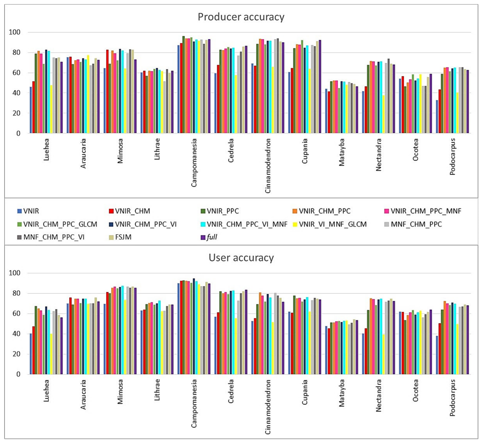[35] reported that LiDAR combined with hyperspectral data increased the classification accuracy of ~2%, with a greater improvement for some tree species. It can also be noticed in this study that the improvement was more evident for some species, such as Ocotea sp./Nectandra megapotamica and Luehea divaricata/Cedrela fissilis. Ocotea sp. class comprises two species of Ocotea genus (O. pulchella and O. puberula), which result in a more diverse spectral behavior. Furthermore Ocotea sp. and Nectandra megapotamica belong to the same family (Lauraceae), having similar spectral characteristics. In this case, the spectral similarity among these tree species can be solved with the inclusion of PPC features. Luehea divaricata and Cedrela fissilis can reach similar heights, thus, the addition of CHM band was not as useful as the inclusion of PPC features to discriminate them. In this case, the PPC features may captured differences in their crown structure, since the former has a wider and denser top with irregular branching, while the latter has a smaller and rounded top, with forked branching [87].

The inclusion of the height information (CHM) also improved accuracies, but to a lesser extent than PPC features: approximately 4% compared with the use of the VNIR bands alone. In the studies of Cho et al. [90], Naidoo et al. [91] and Asner et al. [92], the tree height derived from LiDAR was an important variable for mapping tree species in two completely different forest ecosystems (savannas and tropical forest). On the other hand, Ghosh et al. [12] concluded that there is no significant effect of the height information on tree species classification accuracies in a temperate forest. According to Fassnacht et al. [13], the canopy height per se is not a good predictor to classify tree species as the height of a tree varies with age, site conditions, and competition, and only to a minor degree with species. However, in tropical forests, this predictor can be useful to discriminate species belonging to different successional groups as pioneer, secondary, and climactic, since they tend to have different heights. In this study, there was a great confusion between Mimosa scabrella and Podocarpus lambertii in the datasets without the CHM information. Mimosa scabrella is considered a pioneer species, reaching between 4 and 18 m. Podocarpus lambertii, a late secondary tree, usually is taller, reaching more than 20 m [89]. For this reason, when the height information was incorporated, there was an increase in accuracies of these species, mainly for Mimosa scabrella.

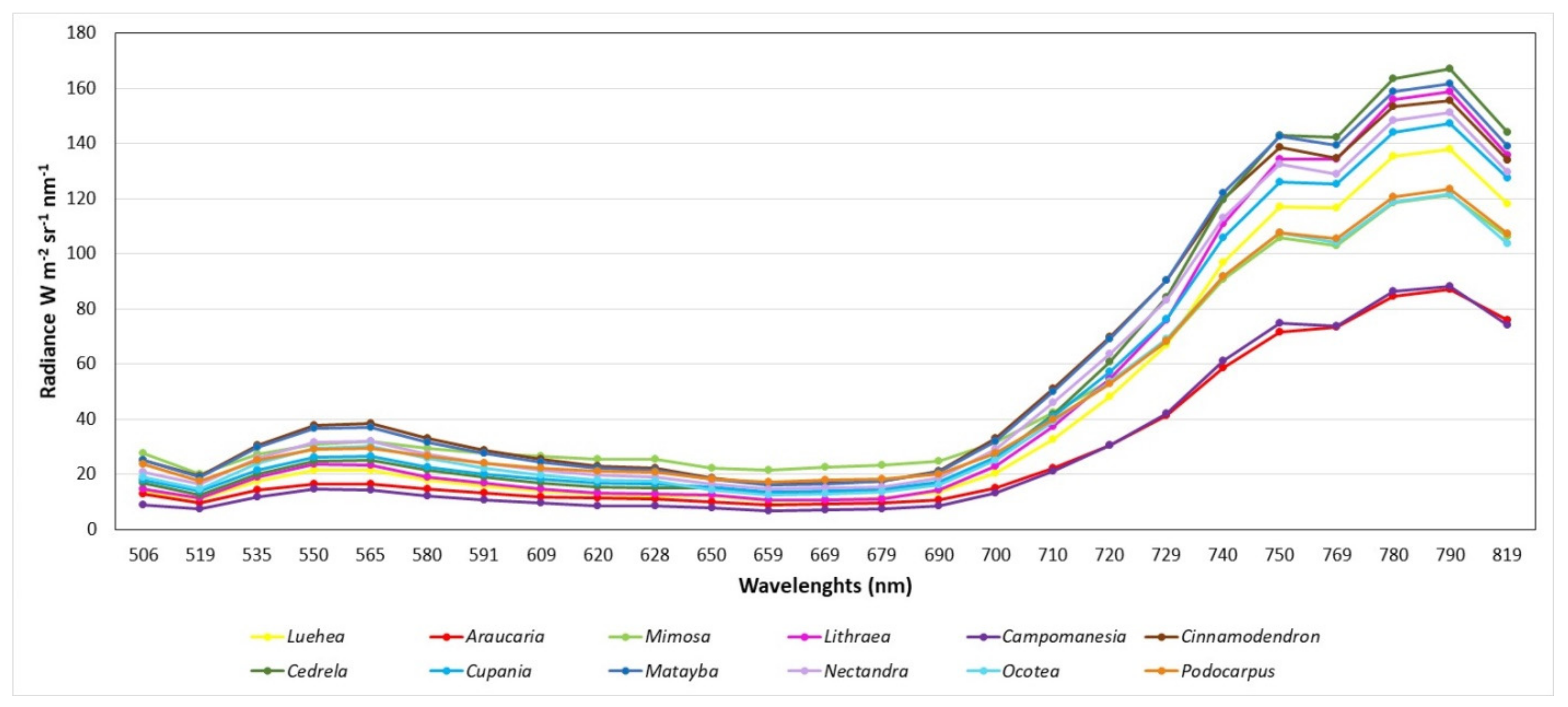
Araucaria angustifolia, the most frequent tree in the study area, presented stable accuracies even with the inclusion of 3D information, showing that even the use of the VNIR bands alone can discriminate this tree species. It can be observed that this species presents the lowest radiance values in all spectra of FPI bands (Figure 3). According to Roberts et al. [93], coniferous trees generally have lower reflectance values in the NIR region compared to broadleaves trees, which is closely related to their needle structure and the higher absorption of coniferous needles. Furthermore, crown size and shape of coniferous trees influence the hemispherical directional reflectance factor (HDRF) and thus their reflectance as well [94]. On the other hand, Podocarpus lambertii, another conifer of the area, tended to be more confused with some broadleaf species. This may have occurred because its shape is not conic as a normal pine, and its branch structure led to confusion with broadleaves species with small leaves, such as Mimosa scabrella.

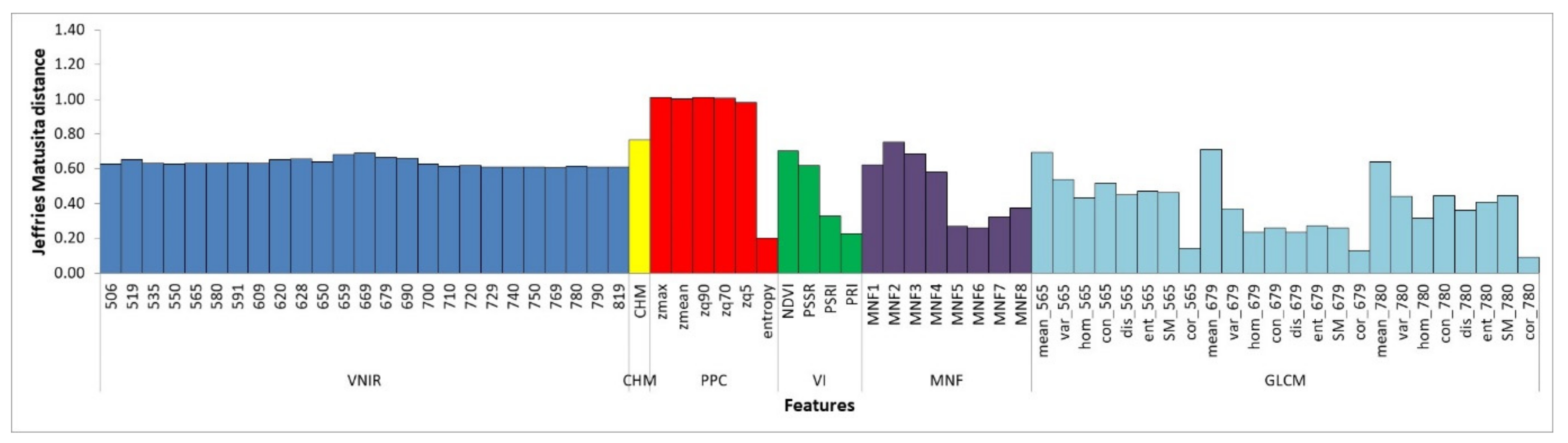
All the VNIR bands showed similar importance according to JM distance (Figure 4). Only slightly higher importance values can be noticed for four bands between 659 and 690 nm. This region included the chlorophyll absorption features, previously reported to contain useful information for the separation of tree species with hyperspectral data [18,54]. The NIR bands, pointed as an important region for tree species classification [15,37], did not stand out in this study. In this region, the tree structure has the strongest impact [95] and the changes in view angle may reduce the relative spectral differences between the species [23]. Furthermore, due to the limited spectral range of the FPI camera (506–819 nm), the complete infrared region (including SWIR) could not be fully tested and assessed.

The inclusion of hyperspectral features (MNF, GLCM, and VIs) in the VNIR_PPC_CHM dataset did not bring significant improvement in accuracy, or even worsened with GLCM features. When all of them were added to the dataset composed solely by VNIR bands (VNIR_VIs_MNF_GLCM) an increase of 1.7% in OA was observed. This increase was also observed when VIs were added to the MNF_PPC_CHM dataset. Ferreira et al. [18] reported an increase in the classification accuracy (of up to 5%) adding the VIs to the VNIR dataset. Maschler et al. [22] found great improvement in tree species classification accuracies when VIs and principal components were aggregated to the classifications, while the inclusion of textural metrics only had a small effect. Although it was not the most important spectral region according to the JM distance, the VIs containing at least one NIR band (PSSR and NDVI) were more important than PSRI and PRI for tree species classification. In the study of Naidoo et al. [93], the NDVI was also scored as one of the most important VIs to classify eight savanna tree species with hyperspectral data. Some studies suggested that band ratios and VIs generated using different band combinations [18,38,89,91] have advantages for species differentiation and biomass estimation because these features can reduce bidirectional reflectance distribution function (BRDF) errors and do not saturate as quickly as single band data [96]. The use of MNF features (MNF_CHM_PPC dataset) instead of VNIR bands (VNIR_CHM_PPC dataset) led to a decrease of 3.1% in OA. Ghosh et al. [12] and Piiroinen et al. [55] reported an improvement when MNF components were used instead of spectral bands, but it is worth noting that in those cases they had hyperspectral data with more than 100 bands. In those cases, MNF transformation reduced the dimensionality and redundancy inherent in high spectral resolution data and, thus, provided better accuracies [12]. Nevertheless, in this study the first four MNF features showed equal or even higher JM values than the VNIR bands.

The use of all VNIR bands, hyperspectral features and CHM and PPC features in the full dataset did not improve the accuracy when compared with the datasets involving the VNIR, PPC, and CHM. In the FS process 48 of the 68 features were selected, resulting in a nonsignificant increase in accuracy when compared with the full dataset. It should be pointed out that studies that performed the FS in hyperspectral data for tree species classification, generally dealt with more than 100 spectral bands [18,22,37,54,55]. However, our hyperspectral data contain only 25 bands, and thus the spectral information is not as redundant as when more than 100 hyperspectral bands are used. Furthermore, according to Fassnacht et al. [13], the FS is commonly applied to reduce the processing time and to enable a meaningful interpretation of the selected predictors, not necessarily resulting in significant increases in classification accuracies. Deng et al. [89], when testing a FS process for tree species classification, stated that for the same feature there were different contribution degrees to species classification in different loops, indicating that the importance of a feature is changeable and greatly depends on the combination with other features. Therefore, it is difficult to determine a combination of features that can benefit all tree species classes at the same time.

5.2. Consideration about the Number of Samples, Tree Species Classes, and Classification Method

Most previous studies concerning tree species classification using UAV (as well as airborne) datasets have been carried out in forests with less-diverse species structure, like boreal and temperate forests (e.g., [12,22,23,37,38,40,56,61,89]), in which is common to find accuracies over 85% (e.g., [12,38,40,89]). However, our findings are consistent with other studies involving airborne hyperspectral data for tree species classification in tropical forest environments. Féret and Asner [21] reached an OA of 73.2% using the pixel-based approach to classify 17 tree species in a Hawaiian tropical forest with airborne hyperspectral data, and 74.9% when they classified only 10 species. When testing machine learning algorithms to classify eight tree species of a subtropical forest in Brazil, Ferreira et al. [18] achieved an average classification accuracy of 70% using the VNIR hyperspectral bands. In that case, the inclusion of shortwave infrared (SWIR) bands increased the accuracy to 84%. Using hyperspectral data with visible, NIR and SWIR bands, Clark and Roberts [15] reached an OA of 71.5% in the pixel-based approach to classify seven emerged-canopy species in a tropical forest in Costa Rica. Regarding studies involving other high diverse environments, Piironen et al. [55] reached 57% of OA when classifying 31 tree species in a diverse agroforestry landscape in Africa. Graves et al. [97] classified 20 tree species and one mixed-species class in a tropical agricultural landscape in Panama and reported an OA of 62%.

According to Ferét and Asner [21], the minimum number of samples per species required to perform optimal classification is a limiting factor in tropical forest studies due to the difficulty and high cost of tree localization on the ground. Our study, similarly to other studies involving the classification of a considerable number of tree species, e.g., Féret and Asner [21], Tuominen et al. [24] and Piiroinen et al. 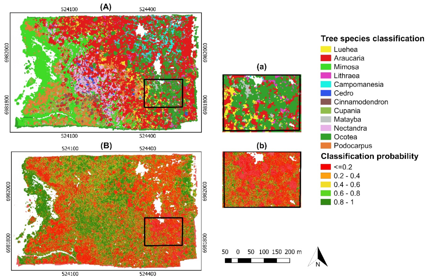[55], had only few ITC samples for some classes. This, coupled with the fact that not all the species were considered in the SVM model, is an obstacle to extrapolate the classification model over the entire area, since it may result in a map with many uncertainties (Figure 6). Even so, this kind of map could be used in some general ecological applications such as assessing patterns of species composition and abundance across environmental gradients or land management units, identification of areas of high or low tree cover and species diversity, identification of ecological groups of tree species (as pioneer, secondary, and climax) assisting the successional forest stage classification, and providing landscape estimates of aboveground biomass [97]. For more focused applications where accurate predictions of species location and identity is needed, such as monitoring endangered tree species (e.g., Araucaria angustifolia and Cedrela fissilis), classification and mapping errors may be too large. For these applications, techniques such as semisupervised methods where a focal group of species is identified from a background of unknown species [16,98], can be a better approach [97].

The SVM classifier proved to be a suitable choice for this study, maintaining a relatively stable performance with few samples, even when the complexity of the datasets increased with the addition of several features. This algorithm has proved to be a promising approach for tree species classification, having a similar [12,40] or even surpassing the Random Forest algorithm performance [18,37,55,56,89,99]. Some studies showed that SVM performs better than RF in the presence of small or imbalanced datasets. In this situation, RF tends to focus more on the prediction accuracy of the majority class, which often results in poor accuracy for the minority classes [37,100]. On the other hand, RF has the advantage of having fewer parameters to be tuned, a lower computational cost [37] and it is less affected by correlated variables [15].

This work adopted a pixel-based approach for tree species level classification. According to Heinzel and Koch [36], object-based approaches using individual ITCs as classification units may reduce the negative effects of spectral variability of pixels. However, most of studies that indicated advantages in object-based approaches did not use the ITC as a classification unit, but instead grouped the pixels into segments after the classification, using a majority class rule procedure [18,20,21]. Clark and Roberts [15] compared the object-based approach, composed by the mean spectra of each ITC, with pixel and majority rule approaches. The pixel classification had roughly the same performance (~70% OA) as when using the average spectra from ITCs, however the pixel-majority classification had much better accuracy, 87%. Féret and Asner [21] reached better results in an object-based approach (79.6%) when compared with the pixel classification (74.9% of OA) to classify tree species in a tropical forest. However, for the object-based classification, they had to reduce the number of classes from 17 to 10, due to the limited number of pixels and the tree crowns labeled to train the classifiers. Furthermore, according to the authors, the segmentation did not delineate ITCs correctly, but each crown was composed by several segments.

Indeed, a proper ITC delineation in a high diversity tropical forest is a complicated task, because of its complex structure. In this sense, most of the published studies focusing on ITC delineation are concentrated in coniferous forests, since most algorithms assume a basic conical crown shape, which is more appropriate for conifers [101]. If an object-based methodology can integrate spectral information with crown-shape parameters, it will greatly assist the process of tree mapping and more accurately fit the needs of tropical forest ecosystem management [10,67]. Therefore, the production of reliable species maps in a high diversity tropical forest with object-based approaches is still a topic to be explored.

5.3. Considerations about the UAV-Camera

The use an UAV hyperspectral camera proved to be a cheap and fast way to acquire data for tree species classification in a highly diverse forest. When considering different UAV sensors, the advantages of the image frame approach over the traditional push broom or whiskbroom scanning approaches include the possibility to collect image blocks with stereoscopic multiple object views maintaining the geometric and radiometric constraints provided by the rigid rectangular image geometry [25]. On the other hand, the current first-generation frame format hyperspectral cameras have a poorer spectral resolution (FWHM of 10 to 30 nm), and less spectral bands respect to more mature push broom techniques, which typically provide hundreds of spectral bands with FWHMs of 2 to 10 nm [102]. In the future, the spectral performance of the FPI cameras is expected to improve, and the latest commercial cameras already offer improved performances [29,102].

6. Conclusions

This study investigated the ability of UAV-based photogrammetry and hyperspectral imaging for tree species classification in a subtropical forest area. The results were very promising, since the VNIR bands associated with PPC features had the potential to provide accurate results to classify 12 tree species of a highly diverse and complex forest. The inclusion of PPC features to the VNIR bands increased the OA of 11%. The best result was achieved when the CHM and VIs were combined with the VNIR_PPC dataset, reaching an OA of 72.4% and a Kappa index of 0.70.

The OA increased by 4.2% when a CHM band generated subtracting the photogrammetric dense surface model and the DTM derived from LiDAR data was added to the VNIR dataset. Among the other hyperspectral features (VIs, MNF and GLCM), two VIs (NDVI and PSSR), the first four MNF and the textural mean of the bands centered at 565 nm and 679 nm showed to be more important to discriminate the tree species according to the JM distance. In the same way, the spectral bands located in the red region presented a slightly higher JM distance values than other bands. The FS process had no significant effect in accuracies, since our original dataset can be considered small when compared with traditional airborne hyperspectral data.

The SVM method proved to be a good classifier for the tree species recognition task, even in the presence of a small sample dataset. In further studies, a feasible approach for improving the classification performance might be to explore ITC delineation methods for tropical forest environments, associated with an object-based classification at the ITC level, and also to explore methods focused on imbalanced sample datasets.

References

1. Slik, J.W.F.; Arroyo-Rodrguez, V.; Aiba, S.-I.; Alvarez-Loayza, P.; Alves, L.F.; Ashton, P.; Balvanera, P.; Bastian, M.L.; Bellingham, P.J.; van den Berg, E.; et al. An estimate of the number of tropical tree species. Proc. Natl. Acad. Sci. USA 2015, 112, 7472–7477. [Google Scholar] [CrossRef] [PubMed] [Green Version]
2. Zhang, Z.; Zang, R.; Wang, G.; Huang, X. Classification of landscape types based on land cover, successional stages and plant functional groups in a species-rich forest in Hainan Island, China. Trop. Conserv. Sci. 2016, 9, 135–152. [Google Scholar] [CrossRef]
3. Viana, V.; Tabanez, A.J. Biology and Conservation of Forest. Fragments in Brasilian Atlantic Moist Forest. In Forest Patches in Tropical Landscapes; Scheilas, J., Greenberg, R., Eds.; Island Press: Washington, DC, USA, 1996. [Google Scholar]
4. Ribeiro, M.; Metzger, J.P.; Martensen, A.C.; Ponzoni, F.J.; Hirota, M.M. The Brazilian Atlantic Forest: How much is left, and how is the remaining forest distributed? Implications for conservation. Biol. Conserv. 2009, 142, 1141–1153. [Google Scholar] [CrossRef]
5. Joly, C.A.; Metzger, J.P.; Tabarelli, M. Experiences from the Brazilian Atlantic Forest: Ecological findings and conservation initiatives. New Phytol. 2014, 204, 459–473. [Google Scholar] [CrossRef]
6. Martinelli, G.; Moraes, M.A. Livro Vermelho da Flora do Brasil; Centro Nacional de Conservação da Flora: Rio de Janeiro, Brazil, 2013. [Google Scholar]
7. Paglia, A.P.; Fonseca, G.A.; Silva, J.M. A Fauna Brasileira Ameaçada de Extinção: Síntese taxonômica e geográfica. In Livro Vermelho da Fauna Brasileira Ameaçada de Extinção; Machado, A.B.M., Drummond, G.M., Paglia, A.O., Eds.; Biodiversidade, Ministério do Meio Ambiente, Ministério da Educação: Brasilia, Brazil, 2008; pp. 63–70. [Google Scholar]
8. Rezende, C.L.; Scarano, F.R.; Assad, E.D.; Joly, C.A.; Metzger, J.P.; Strassburg, B.B.N.; Tabarelli, M.; Fonseca, G.A.; Mittermeier, R.A. From hotspot to hopespot: An opportunity for the Brazilian Atlantic Forest. Perspect. Ecol. Conserv. 2018, 16, 208–214. [Google Scholar] [CrossRef]
9. Colombo, A.F.; Joly, C.A. Brazilian Atlantic Forest lato sensu: The most ancient Brazilian forest, and a biodiversity hotspot, is highly threatened by climate change. Braz. J. Biol. 2010, 70, 697–708. [Google Scholar] [CrossRef]
10. Wagner, F.H.; Ferreira, M.P.; Sanchez, A.; Hirye, M.C.M.; Zortea, M.; Gloor, E.; Phillips, O.L.; de Souza Filho, C.R.; Shimabukuro, Y.E.; Aragão, L.E.O.C. Individual tree crown delineation in a highly diverse tropical forest using very high resolution satellite images. ISPRS J. Photogramm. Remote Sens. 2018, 145, 362–377. [Google Scholar] [CrossRef]
11. Dalponte, M.; Bruzzone, L.; Gianelle, D. Fusion of hyperspectral and LIDAR remote sensing data for classification of complex forest areas. IEEE Trans. Geosci. Remote Sens. 2008, 46, 1416–1427. [Google Scholar] [CrossRef]
12. Ghosh, A.; Fassnacht, E.F.; Joshi, P.K.; Koch, B. A framework for mapping tree species combining hyperspectral and LiDAR data: Role of selected classifiers and sensor across three spatial scales. Int. J. Appl. Earth Obs. Geoinf. 2014, 26, 49–63. [Google Scholar] [CrossRef]
13. Fassnacht, F.E.; Latifi, H.; Stereczak, K.; Modzelewska, A.; Lefsky, M.; Waser, L.T.; Straub, C.; Ghosh, A. Review of studies on tree species classification from remotely sensed data. Remote Sens. Environ. 2016, 186, 64–87. [Google Scholar] [CrossRef]
14. Clark, M.L.; Roberts, D.A.; Clark, D.B. Hyperspectral discrimination of tropical rain forest tree species at leaf to crown scales. Remote Sens. Environ. 2005, 96, 375–398. [Google Scholar] [CrossRef]
15. Clark, M.L.; Roberts, D.A. Species-level differences in hyperspectral metrics among tropical rainforest trees as determined by a tree-based classifier. Remote Sens. 2012, 4, 1820–1855. [Google Scholar] [CrossRef]
16. Baldeck, C.A.; Asner, G.P.; Martin, R.E.; Anderson, C.B.; Knapp, D.E.; Kellner, J.R.; Wright, S.J. Operational tree species mapping in a diverse tropical forest with airborne imaging spectroscopy. PLoS ONE 2015, 10, e0118403. [Google Scholar] [CrossRef]
17. Cao, L.; Coops, N.C.; Innes, J.L.; Dai, J.; Ruan, H. Tree species classification in subtropical forests using small-footprint full-waveform LiDAR data. Int. J. Appl. Earth Obs. Geoinf. 2016, 49, 39–51. [Google Scholar] [CrossRef]
18. Ferreira, M.P.; Zortea, M.; Zanotta, D.C.; Shimabukuro, Y.E.; de Souza Filho, C.R. Mapping tree species in tropical seasonal semi-deciduous forests with hyperspectral and multispectral data. Remote Sens. Environ. 2016, 179, 66–78. [Google Scholar] [CrossRef]
19. Shen, X.; Cao, L. Tree-Species Classification in Subtropical Forests Using Airborne Hyperspectral and LiDAR Data. Remote Sens. 2017, 9, 1180. [Google Scholar] [CrossRef]
20. Dalponte, M.; Ørka, H.O.; Gobakken, T.; Gianelle, D.; Næsset, E. Tree species classification in boreal forests with hyperspectral data. IEEE Trans. Geosci. Remote Sens. 2013, 51, 2632–2645. [Google Scholar] [CrossRef]
21. Féret, J.; Asner, G.P. Tree species discrimination in tropical forests using airborne imaging spectroscopy. IEEE Trans. Geosci. Remote Sens. 2013, 51, 73–84. [Google Scholar] [CrossRef]
22. Maschler, J.; Atzberger, C.; Immitzer, M. Individual Tree Crown Segmentation and Classification of 13 Tree Species Using Airborne Hyperspectral Data. Remote Sens. 2018, 10, 1218. [Google Scholar] [CrossRef]
23. Nevalainen, O.; Honkavaara, E.; Tuominen, S.; Viljanen, N.; Hakala, T.; Yu, X.; Hyypa, J.; Saari, H.; Polonen, I.; Imai, N.N.; et al. Individual Tree Detection and Classification with UAV-Based Photogrammetric Point Clouds and Hyperspectral Imaging. Remote Sens. 2017, 9, 185. [Google Scholar] [CrossRef]
24. Tuominen, S.; Näsi, R.; Honkavaara, E.; Balazs, A.; Hakala, T.; Viljanen, N.; Pölönen, I.; Saari, H.; Ojanen, H. Assessment of Classifiers and Remote Sensing Features of Hyperspectral Imagery and Stereo-Photogrammetric Point Clouds for Recognition of Tree Species in a Forest Area of High Species Diversity. Remote Sens. 2018, 10, 714. [Google Scholar] [CrossRef]
25. Honkavaara, E.; Saari, H.; Kaivosoja, J.; Pölönen, I.; Hakala, T.; Litkey, P.; Mäkynen, J.; Pesonen, L. Processing and Assessment of Spectrometric, Stereoscopic Imagery Collected Using a Lightweight UAV Spectral Camera for Precision Agriculture. Remote Sens. 2013, 5, 5006–5039. [Google Scholar] [CrossRef] [Green Version]
26. Paneque-Gálvez, J.; Mccall, M.K.; Napoletano, B.M.; Wich, S.A.; Koh, L.P. Small drones for community-based forest monitoring: An assessment of their feasibility and potential in tropical areas. Forests 2014, 5, 1481–1507. [Google Scholar] [CrossRef]
27. Nex, F.; Remondino, F. UAV for 3D mapping applications: A review. Appl. Geomat. 2014, 6, 1–15. [Google Scholar] [CrossRef]
28. Matese, A.; Toscano, P.; Di Gennaro, S.; Genesio, L.; Vaccari, F.; Primicerio, J.; Belli, C.; Zaldei, A.; Bianconi, R.; Gioli, B. Intercomparison of UAV, aircraft and satellite remote sensing platforms for precision viticulture. Remote Sens. 2015, 7, 2971–2990. [Google Scholar] [CrossRef]
29. Aasen, H.; Honkavaara, E.; Lucieer, A.; Zarco-Tejada, P.J. Quantitative Remote Sensing at Ultra-High Resolution with UAV Spectroscopy: A Review of Sensor Technology, Measurement Procedures, and Data Correction Workflows. Remote Sens. 2018, 10, 1091. [Google Scholar] [CrossRef]
30. Aasen, H.; Burkart, A.; Bolten, A.; Bareth, G. Generating 3D hyperspectral information with lightweight UAV snapshot cameras for vegetation monitoring: From camera calibration to quality assurance. ISPRS J. Photogramm. Remote Sens. 2015, 108, 245–259. [Google Scholar] [CrossRef]
31. Näsi, R.; Honkavaara, E.; Lyytikäinen-Saarenmaa, P.; Blomqvist, M.; Litkey, P.; Hakala, T.; Viljanen, N.; Kantola, T.; Tanhuanpää, T.; Holopainen, M. Using UAV-based photogrammetry and hyperspectral imaging for mapping bark beetle damage at tree-level. Remote Sens. 2015, 7, 15467–15493. [Google Scholar] [CrossRef]
32. Lu, D.; Weng, Q. A Survey of Image Classification Methods and Techniques for Improving Classification Performance. Int. J. Remote Sens. 2007, 28, 823–870. [Google Scholar] [CrossRef]
33. Mountrakis, G.; Im, J.J.; Ogole, C. Support vector machines in remote sensing: A review. ISPRS J. Photogramm. Remote Sens. 2011, 66, 247–259. [Google Scholar] [CrossRef]
34. Melgani, F.; Bruzzone, L. Classification of hyperspectral remote sensing images with support vector machines. IEEE Trans. Geosci. Remote Sens. 2004, 42, 1778–1790. [Google Scholar] [CrossRef] [Green Version]
35. Jones, T.G.; Coops, N.C.; Sharma, T. Assessing the utility of airborne hyperspectral and LiDAR data for species distribution mapping in the coastal Pacific Northwest, Canada. Remote Sens. Environ. 2010, 114, 2841–2852. [Google Scholar] [CrossRef]
36. Heinzel, J.; Koch, B. Investigating multiple data sources for tree species classification in temperate forest and use for single tree delineation. Int. J. Appl. Earth Obs. Geoinf. 2012, 18, 101–110. [Google Scholar] [CrossRef]
37. Dalponte, M.; Bruzzone, L.; Gianelle, D. Tree species classification in the southern alps based on the fusion of very high geometrical resolution multispectral/hyperspectral images and LiDAR data. Remote Sens. Environ. 2012, 123, 258–270. [Google Scholar] [CrossRef]
38. Dalponte, M.; Ørka, H.O.; Ene, L.T.; Gobakken, T.; Naesset, E. Tree crown delineation and tree species classification in boreal forests using hyperspectral and ALS data. Remote Sens. Environ. 2014, 140, 306–317. [Google Scholar] [CrossRef]
39. Heenkenda, M.K.; Joyce, E.K.; Maier, S.W.; Bartolo, R. Mangrove Species Identification: Comparing WorldView-2 with Aerial Photographs. Remote Sens. 2014, 6, 6064–6088. [Google Scholar] [CrossRef] [Green Version]
40. Ballanti, L.; Blesius, L.; Hines, E.; Kruse, B. Tree Species Classification Using Hyperspectral Imagery: A Comparison of Two Classifiers. Remote Sens. 2016, 8, 445. [Google Scholar] [CrossRef]
41. Peel, M.C.; Finlayson, B.L.; McMahon, T.A. Updated world map of the Köppen-Geiger climate classification. Hydrol. Earth Syst. Sci. 2007, 11, 1633–1644. [Google Scholar] [CrossRef]
42. Kalacska, M.; Bohlman, S.; Sanchez-Azofeifa, G.A.; Castro-Esau, K.; Caelli, T. Hyperspectral discrimination of tropical dry forest lianas and trees: Comparative data reduction approaches at the leaf and canopy levels. Remote Sens. Environ. 2007, 109, 406–415. [Google Scholar] [CrossRef]
43. Vibrans, A.C.; Sevgnani, L.; Lingner, D.V.; de Gasper, A.L.; Sabbagh, S. Inventário florístico florestal de Santa Catarina (IFFSC): Aspectos metodológicos e operacionais. Pesqui. Florest. Bras. 2010, 30, 291. [Google Scholar] [CrossRef]
44. Bianchi, J.S.; Bento, C.M.; Kersten, R.A. Vascular epiphytes of an Araucaria-Atlantic forest ecotone at Pico do Marumbi State Park, Southern Brazil. Estud. Biol. 2012, 34, 37–44. [Google Scholar] [CrossRef]
45. Senop. Datasheet VIS-NIR Snapshot Hyperspectral Camera for UAVs. Snapshot Hyperspectral Camera. Available online: http://view.24mags.com/mera/datasheet-hyperspectralcamera (accessed on 2 August 2018).
46. Miyoshi, G.T.; Imai, N.N.; Tommaselli, A.M.G.; Honkavaara, E. Impact of reduction of radiometric resolution in hyperspectral images acquired over forest field. In The International Archives of the Photogrammetry, Remote Sensing and Spatial Information Sciences, XLII-1, Proceedings of the ISPRS TC I Mid-term Symposium “Innovative Sensing—From Sensors to Methods and Applications”, Karlsruhe, Germany, 10–12 October 2018; International Society of Photogrammetry and Remote Sensing: Hannover, Germany, 2018. [Google Scholar]
47. Honkavaara, E.; Rosnell, T.; Oliveira, R.; Tommaselli, A. Band registration of tuneable frame format hyperspectral UAV imagers in complex scenes. ISPRS J. Photogramm. Remote Sens. 2017, 134, 96–109. [Google Scholar] [CrossRef]
48. Miyoshi, G.T.; Imai, N.N.; Tommaselli, A.M.G.; Honkavaara, E.; Näsi, R.; Moriya, É.A.S. Radiometric block adjustment of hyperspectral image blocks in the Brazilian environment. Int. J. Remote Sens. 2018, 39, 4910–4930. [Google Scholar] [CrossRef] [Green Version]
49. Oliveira, R.A.; Tommaselli, A.M.; Honkavaara, E. Geometric Calibration of a Hyperspectral Frame Camera. Photogramm. Rec. 2016, 31, 325–347. [Google Scholar] [CrossRef]
50. Isenburg, M. LAStools: Software for Rapid LiDAR Processing. Available online: http://www.cs.unc.edu/~isenburg/lastools/ (accessed on 7 July 2018).
51. Green, A.A.; Berman, M.; Switzer, P.; Craig, M.D. A transformation for ordering multispectral data in terms of image quality with implications for noise removal. IEEE Trans. Geosci. Remote Sens. 1988, 26, 65–74. [Google Scholar] [CrossRef] [Green Version]
52. Haralick, R.M.; Shanmugam, K.; Dinstein, I.H. Textural features for image classification. IEEE Trans. Syst. Man Cybern. 1973, 3, 610–621. [Google Scholar] [CrossRef]
53. Luo, G.; Chen, G.; Tian, L.; Qin, K.; Qian, S.-E. Minimum Noise Fraction versus Principal Component Analysis as a Preprocessing Step for Hyperspectral Imagery Denoising. Can. J. Remote Sens. 2016, 42, 106–116. [Google Scholar] [CrossRef]
54. Fassnacht, F.E.; Neumann, C.; Förster, M.; Buddenbaum, H.; Ghosh, A.; Clasen, A.; Joshi, P.K.; Koch, B. Comparison of feature reduction algorithms for classifying tree species with hyperspectral data on three central European test sites. IEEE J. Sel. Top. Appl. Earth Obs. Remote Sens. 2014, 7, 2547–2561. [Google Scholar] [CrossRef]
55. Piiroinen, R.; Heiskanen, J.; Maeda, E.; Viinikka, A.; Pellikka, P. Classification of Tree Species in a Diverse African Agroforestry Landscape Using Imaging Spectroscopy and Laser Scanning. Remote Sens. 2017, 9, 875. [Google Scholar] [CrossRef]
56. Raczko, E.; Zagajewski, B. Comparison of support vector machine, random forest and neural network classifiers for tree species classification on airborne hyperspectral APEX images. Eur. J. Remote Sens. 2017, 50, 144–154. [Google Scholar] [CrossRef] [Green Version]
57. Sayn-Wittgenstein, L. Recognition of tree species on aerial photographs. In Information Report FMR-X-118; Forest Management Institute: Ottawa, ON, Canada, 1978. [Google Scholar]
58. Johansen, K.; Phinn, S. Mapping structural parameters and species composition of riparian vegetation using IKONOS and Landsat ETM+ data in Australian tropical savannahs. Photogramm. Eng. Remote Sens. 2006, 72, 71–80. [Google Scholar] [CrossRef]
59. Yu, Q.; Gong, P.; Clinton, N.; Biging, G.; Kelly, M.; Schirokauer, D. Object-Based Detailed Vegetation Classification with Airborne High Spatial Resolution Remote Sensing Imagery. Photogramm. Eng. Remote Sens. 2006, 72, 799–811. [Google Scholar] [CrossRef]
60. Mallinis, G.; Koutsias, N.; Tsakiri-Strati, M.; Karteris, M. Object-based classification using Quickbird imagery for delineating forest vegetation polygons in a Mediterranean test site. ISPRS J. Photogramm. Remote Sens. 2008, 63, 237–250. [Google Scholar] [CrossRef]
61. Franklin, S.E.; Ahmed, O.S. Deciduous tree species classification using object-based analysis and machine learning with unmanned aerial vehicle multispectral data. Int. J. Remote Sens. 2018, 39, 5236–5245. [Google Scholar] [CrossRef]
62. Lu, D.; Li, G.; Moran, E.; Kuang, W. A comparative analysis of approaches for successional vegetation classification in the Brazilian Amazon. GISci. Remote Sens. 2014, 51, 695–709. [Google Scholar] [CrossRef]
63. Sothe, C.; Schimalski, M.B.; Liesenberg, V.; de Almeida, C.M. Approaches for classifying successional forest stages in São Joaquim National Park using Landsat-8 and RapidEye images. Bol. Ciênc. Geod. 2017, 23. [Google Scholar] [CrossRef]
64. Lu, D.; Batistella, M.; Li, G.; Moran, E.; Hetrick, S.; Freitas, C.; Dutra, L.; Sant’Anna, S.J.S. Land use/Cover Classification in the Brazilian Amazon using Satellite Images. Braz. J. Agric. Res. 2012, 47, 1185–1208. [Google Scholar] [CrossRef] [PubMed]
65. Attarchi, S.; Gloaguen, R. Classifying Complex Mountainous Forests with L-Band SAR and Landsat Data Integration: A Comparison among Different Machine Learning Methods in the Hyrcanian Forest. Remote Sens. 2014, 6, 3624–3647. [Google Scholar] [CrossRef] [Green Version]
66. Richards, J.A.; Jia, X. Remote Sensing Digital Image Analysis: An Introduction, 4th ed.; Springer: New York, NY, USA, 2006. [Google Scholar]
67. Lin, C.; Popescu, S.C.; Thomson, G.; Tsogt, K.; Chang, C.-I. Classification of Tree Species in Overstorey Canopy of Subtropical Forest Using QuickBird Images. PLoS ONE 2015, 10, e0125554. [Google Scholar] [CrossRef]
68. Rouse, J.W.; Haas, R.H.; Schell, J.A.; Deering, W.D. Monitoring Vegetation Systems in the Great Plains with ERTS; Third ERTS Symp. NASA SP-351; NASA: Houston, TX, USA, 1973; Volume 1, pp. 309–317. [Google Scholar]
69. Gamon, J.A.; Peñuelas, J.; Field, C.B. A narrow-waveband spectral index that tracks diurnal changes in photosynthetic efficiency. Remote Sens. Environ. 1992, 41, 35–44. [Google Scholar] [CrossRef]
70. Merzlyak, M.N.; Gitelson, A.A.; Chivkunova, O.B.; Rakitin, V.Y. Non-destructive optical detection of pigment changes during leaf senescence and fruit ripening. Physiol. Plant. 1999, 106, 135–141. [Google Scholar] [CrossRef] [Green Version]
71. Blackburn, G.A. Spectral indices for estimating photosynthetic pigment concentrations: A test using senescent tree leaves. Int. J. Remote Sens. 1998, 19, 657–675. [Google Scholar] [CrossRef]
72. Roussel, J.R.; Auty, D.; de Boissieu, F.; Meador, A.S. LidR: Airborne LiDAR Data Manipulation and Visualization for Forestry Applications. Available online: https://cran.rproject.org/web/packages/lidR/index.html (accessed on 22 August 2018).
73. R Development Core Team. R: A Language and Environment for Statistical Computing. Available online: http://www.r-project.org (accessed on 20 March 2018).
74. Richards, J.A. Remote Sensing Digital Image Analysis: An Introduction; Springer: Berlin/Heidelberg, Germany, 1993. [Google Scholar]
75. Pudil, P.; Novovicová, J.; Kittler, J. Floating search methods in feature selection. Pattern Recognit. Lett. 1994, 15, 1119–1125. [Google Scholar] [CrossRef]
76. Cortes, C.; Vapnik, V. Support-Vector Networks. Mach. Learn. 1995, 20, 273–297. [Google Scholar] [CrossRef]
77. Adam, E.; Mutanga, O.; Odindi, J.; Abdel-Rahman, E.M. Land-use/cover classification in a heterogeneous coastal landscape using RapidEye imagery: Evaluating the performance of random forest and support vector machines classifiers. Int. J. Remote Sens. 2014, 35, 3440–3458. [Google Scholar] [CrossRef]
78. Steinwart, I.; Christmann, A. Support Vector Machines; Springer: New York, NY, USA, 2008. [Google Scholar]
79. Huang, C.; Davis, L.S.; Townshend, J.R.G. An assessment of support vector machines for land cover classification. Remote Sens. 2002, 23, 725–749. [Google Scholar] [CrossRef]
80. Duro, D.C.; Franklin, S.E.; Dube, M.G. A comparison of pixel-based and object-based image analysis with selected machine learning algorithms for the classification of agricultural landscapes using SPOT-5 HRG imagery. Remote Sens. Environ. 2012, 118, 259–272. [Google Scholar] [CrossRef]
81. Burges, C.J. A tutorial on support vector machines for pattern recognition. Data Min. Knowl. Discov. 1998, 2, 121–167. [Google Scholar] [CrossRef]
82. Li, W.; Du, Q. Support vector machine with adaptive composite kernel for hyperspectral image classification. In Satellite Data Compression, Communications, and Processing XI, Proceedings of the SPIE Sensing Technology + Applications, Baltimore, MD, USA, 20–24 April 2015; SPIE: Bellingham, WA, USA, 2015. [Google Scholar]
83. Hurlbert, S.H. Pseudoreplication and the Design of Ecological Field Experiments. Ecol. Monogr. 1984, 54, 187–211. [Google Scholar] [CrossRef] [Green Version]
84. Brovelli, M.A.; Crespi, M.; Fratarcangeli, F.; Giannone, F.; Realini, E. Accuracy assessment of high resolution satellite imagery orientation by leave-one-out method. ISPRS J. Photogramm. Remote Sens. 2008, 63, 427–440. [Google Scholar] [CrossRef]
85. Cohen, J. A coefficient of agreement for nominal scales. Educ. Psychol. Meas. 1960, 20, 37–46. [Google Scholar] [CrossRef]
86. Skidmore, A.K. Accuracy Assessment of Spatial Information. In Spatial Statistics for Remote Sensing; Stein, A., van der Meer, F.D., Gorte, B., Eds.; Kluwer Academic Publishers: Dordrecht, The Netherlands, 1999; pp. 197–209. [Google Scholar]
87. Lorenzi, H. Árvores Brasileiras: Manual de Identificação e Cultivo de Plantas Arbóreas Nativas do Brasil; Plantarum: Nova Odessa, Brazil, 1992; p. 351. [Google Scholar]
88. Soares, R.V. Considerações sobre a regeneração natural da Araucaria angustifólia. Floresta 1979, 10, 11–18. [Google Scholar] [CrossRef]
89. Deng, S.; Katoh, M.; Yu, X.; Hyyppä, J.; Gao, T. Comparison of Tree Species Classifications at the Individual Tree Level by Combining ALS Data and RGB Images Using Different Algorithms. Remote Sens. 2016, 8, 1034. [Google Scholar] [CrossRef]
90. Cho, M.A.; Mathieu, R.; Asner, G.P.; Naidoo, L.; Van Aardt, J.; Ramoelo, A.; Debba, P.; Wessels, K.; Main, R.; Smit, I.P.J.; et al. Mapping tree species composition in South African savannas using an integrated airborne spectral and LiDAR system. Remote Sens. Environ. 2012, 125, 214–226. [Google Scholar] [CrossRef]
91. Naidoo, L.; Cho, M.A.; Mathieu, R.; Asner, G. Classification of savanna tree species, in the Greater Kruger National Park region, by integrating hyperspectral and LiDAR data in a Random Forest data mining environment. ISPRS J. Photogramm. Remote Sens. 2012, 69, 167–179. [Google Scholar] [CrossRef]
92. Asner, G.P.; Knapp, D.E.; Kennedy-Bowdoin, T.; Jones, M.O.; Martin, R.E.; Boardman, J.; Hughes, R.F. Invasive species detection in Hawaiian Rainforests using Airborne Imaging Spectroscopy and LiDAR. Remote Sens. Environ. 2008, 112, 1942–1955. [Google Scholar] [CrossRef]
93. Roberts, D.A.; Ustin, S.L.; Ogunjemiyo, S.; Greenberg, J.; Dobrowski, S.Z.; Chen, J.; Hinckley, T.M. Spectral and Structural Measures of Northwest Forest Vegetation at Leaf to Landscape Scales. Ecosystems 2004, 7, 545–562. [Google Scholar] [CrossRef]
94. Rautiainen, M.; Stenberg, P. Application of photon recollision probability in coniferous canopy reflectance simulations. Remote Sens. Environ. 2005, 96, 98–107. [Google Scholar] [CrossRef]
95. Ponzoni, F.J.; Shimabukuro, Y.E.; Kuplich, T.M. Sensoriamento Remoto da Vegetação, 2nd ed.; Oficina de Textos: São Paulo, Brazil, 2012. [Google Scholar]
96. Colgan, M.S.; Baldeck, C.A.; Féret, J.-B.; Asner, G.P. Mapping savanna tree species at ecosystem scales using support vector machine classification and BRDF correction on airborne hyperspectral and LiDAR data. Remote Sens. 2012, 4, 3462–3480. [Google Scholar] [CrossRef]
97. Graves, S.J.; Asner, G.P.; Martin, R.E.; Anderson, C.B.; Colgan, M.S.; Kalantari, L.; Bohlman, S. Tree species abundance predictions in a tropical agricultural landscape with a supervised classification model and imbalanced data. Remote Sens. 2016, 8, 161. [Google Scholar] [CrossRef]
98. Baldeck, C.A.; Asner, G.P. Single-species detection with airborne imaging spectroscopy data: A comparison of support vector techniques. IEEE J. Sel. Top. Appl. Earth Obs. Remote Sens. 2014, 8, 2501–2512. [Google Scholar] [CrossRef]
99. Burai, P.; Deak, B.; Valko, O.; Tomor, T. Classification of herbaceous vegetation using airborne hyperspectral imagery. Remote Sens. 2015, 7, 2046–2066. [Google Scholar] [CrossRef]
100. Chen, C.; Liaw, A.; Breiman, L. Using Random Forest to Learn Imbalanced Data; University of California, Berkeley: Berkeley, CA, USA, 2004. [Google Scholar]
101. Zhen, Z.; Quackenbush, L.J.; Zhang, L. Trends in Automatic Individual Tree Crown Detection and Delineation—Evolution of LiDAR Data. Remote Sens. 2016, 8, 333. [Google Scholar] [CrossRef]
102. Honkavaara, E.; Eskelinen, M.A.; Pölönen, I.; Saari, H.; Ojanen, H.; Mannila, R.; Holmlund, C.; Hakala, T.; Litkey, P.; Rosnell, T.; et al. Remote Sensing of 3-D Geometry and Surface Moisture of a Peat Production Area Using Hyperspectral Frame Cameras in Visible to Short-Wave Infrared Spectral Ranges Onboard a Small Unmanned Airborne Vehicle (UAV). IEEE Trans. Geosci. Remote Sens. 2016, 54. [Google Scholar] [CrossRef]
Figure 1. Study area location. (A) Santa Catarina State. (B) Curitibanos municipality. (C) Hyperspectral UAV image R (535 nm) G (769 nm) B (679 nm). (D) Digital Terrain Model.
Remotesensing 11 01338 g001
Figure 2. Tree species classes delimitated in the unmanned aerial vehicle (UAV)-RGB image and the corresponding UAV-hyperspectral image.
Remotesensing 11 01338 g002
Figure 3. Spectral radiance curves of the tree species obtained by the Fabry–Perot interferometer (FPI) camera.
Remotesensing 11 01338 g003
Figure 4. Jeffries–Matusita distance mean among all classes according to each feature.
Remotesensing 11 01338 g004
Figure 5. Producer’s and user’s accuracies of tree species classes according to the dataset.
Remotesensing 11 01338 g005
Figure 6. Classified (A) and probability map (B) with VNIR_CHM_PPC_VI dataset. Zoom (a,b) demonstrate a high uncertainty area classified as Ocotea sp.
Remotesensing 11 01338 g006