In Situ and Satellite Sea Surface Salinity in the Algerian Basin Observed through ABACUS Glider Measurements and BEC SMOS Regional Products

Abstract

The Algerian Basin is a key area for the general circulation in the western Mediterranean Sea. The basin has an intense inflow/outflow regime with complex circulation patterns, involving both fresh Atlantic water and more saline Mediterranean water. Several studies have demonstrated the advantages of the combined use of autonomous underwater vehicles, such as gliders, with remotely sensed products (e.g., altimetry, MUR SST) to observe meso- and submesoscale structures and their properties. An important contribution could come from a new generation of enhanced satellite sea surface salinity (SSS) products, e.g., those provided by the Soil Moisture and Ocean Salinity (SMOS) mission. In this paper, we assess the advantages of using Barcelona Expert Center (BEC) SMOS SSS products, obtained through a combination of debiased non-Bayesian retrieval, DINEOF (data interpolating empirical orthogonal functions) and multifractal fusion with high resolution sea surface temperature (OSTIA SST) maps. Such an aim was reached by comparing SMOS Level-3 (L3) and Level-4 (L4) SSS products with in situ high resolution glider measurements collected in the framework of the Algerian Basin Circulation Unmanned Survey (ABACUS) observational program conducted in the Algerian Basin during falls 2014–2016. Results show that different levels of confidence between in situ and satellite measurements can be achieved according to the spatial scales of variability. Although SMOS values slightly underestimate in situ observations (mean difference is −0.14 (−0.11)), with a standard deviation of 0.25 (0.26) for L3 (L4) products), at basin scale, the enhanced SMOS products well represent the salinity patterns described by the ABACUS data.

1. Introduction

The Algerian Basin (hereafter AB) is a wide and deep transit region located in the western Mediterranean Sea, of which it constitutes the southern part. This basin is about 750 km wide at 38.5°N between the coast of Spain and the Sardinia Channel, while the latitudinal extension between the Algerian Coast and the Balearic Islands (at 2.5°E) is about 250 km. The AB is characterized by the presence at surface levels of both fairly fresh water coming from the Atlantic (Atlantic water, hereafter AW) and more saline waters, which typically reside in the Mediterranean region (Mediterranean water, MW). According to different stages of mixing, geographical position, and residence time in the Mediterranean Sea, AW properties vary across this basin, ranging between 14–27 °C and 36.5–38.0, in terms of potential temperature and salinity respectively. The Levantine intermediate water (LIW), typified by subsurface temperature and salinity maxima, is also present at intermediate levels (400–900 m depth), with a typical potential temperature lower than 13.5 °C and a salinity of about 38.5. The western Mediterranean deep water (WMDW) occupies deeper layers, being characterized by temperatures of about 13 °C and salinity values ranging between 38 and 38.9 [1,2,3].

The general circulation of these water masses is strongly influenced by both the intense inflow/outflow regime [2,4] and the complex circulation patterns [5,6,7], which act in the AB at different spatial and temporal scales [8]. In particular, AW carried by the Algerian Current (AC) generates several fresh-core coastal eddies that propagate downstream [9,10] and promote water mass mixing, thus affecting the spatial distribution of salinity, and, consequently, the Mediterranean Sea surface circulation. These mesoscale energetic structures also have marked repercussions on nutrient injection (removal) into (out of) the euphotic layer. In fact, a large anticorrelation between sea level anomalies and phytoplankton biomass has been previously observed in the AB [11], thus suggesting a clear response of biological activity to the shoaling/deepening of isopycnals [12]. As part of the southwestern Mediterranean region, this basin is also known to be particularly responsive to climate change [13,14], and the Mediterranean waters flowing in this area have already shown significant trends at different depths in both temperature and salinity [15,16,17,18].

Moreover, the convection processes occurring in the northwestern Mediterranean feed the formation of western Mediterranean deep water (hereafter WMDW), which contributes to the Mediterranean thermohaline circulation. These deep waters have become saltier and warmer for at least the past 40 years at rates of about 0.015 and 0.04 °C per decade [19], but the budget of salt involved in the formation of WMDW is still under investigation [20,21,22]. WMDW convection is also associated with the vertical mixing that enriches the surface layer with critical nutrients, thus contributing to spring bloom and primary production rates [23]. These phenomena have been intensively studied in recent years, but a complete knowledge of the mechanisms acting in the AB is still pending. Thus, both accurate observations of surface salinity and reliable estimates of salt budgets are essential to support the scientific efforts to model past and future evolution of Mediterranean climate and give an answer to these open questions.

Although the Mediterranean region is strongly affected by radio frequency interference (RFI) and systematic biases due to the coast contamination, European Space Agency (ESA) soil moisture and ocean salinity (SMOS) [24,25] sea surface salinity (SSS) products have been already used to detect mesoscale structures and reconstruct coherent currents in the AB [26]. Nevertheless, evident biases were found when analyzing SSS values in comparison with Argo floats. To overcome these problems, a new set of SMOS SSS enhanced products [27] has been obtained at the Barcelona Expert Center (BEC) through a combination of debiased non-Bayesian retrieval [28], deletion of time-dependent residual biases by means of DINEOF (data interpolating empirical orthogonal functions) [29], and multifractal fusion with high resolution sea surface temperature (OSTIA SST) maps [30].

Several studies have assessed the advantages of multiplatform ocean monitoring over different scales, including mesoscale, and at different latitudes [31,32,33,34,35,36,37]. Recent experiments demonstrated that combining new technologies for in situ data collection, mainly autonomous underwater vehicles (AUVs), and reliable satellite data in the AB (e.g., [12,38,39]), provides useful contributions to properly address state-of-the-art scientific challenges [40,41,42]. AUVs allow the collection of high resolution physical and biochemical data along the water column from surface to 975 m depth [17], while their use in combination with remote sensing observations provides a better understanding of basin-scale processes, such as those influencing the southwestern Mediterranean Sea dynamics [38,43].

Furthermore, information collected through AUVs in the AB has already confirmed their usefulness in the validation of new satellite altimetry products, e.g., those coming from the SARAL/AltiKa [7] and the new Sentinel-3 mission [44]; AUV activities in the AB are also fully involved in the framework of upcoming satellite missions, such as the Surface Water and Ocean Topography (SWOT) wide-swath radar interferometer [45,46].

In such a context, this study compares ABACUS (Algerian Basin Circulation Unmanned Survey) in situ high resolution glider measurements collected in the AB during fall 2014–2016 with co-located SMOS enhanced SSS L3 and L4 products, provided by BEC, in order to confirm that retrieving reliable SMOS SSS in the Mediterranean region is indeed possible.

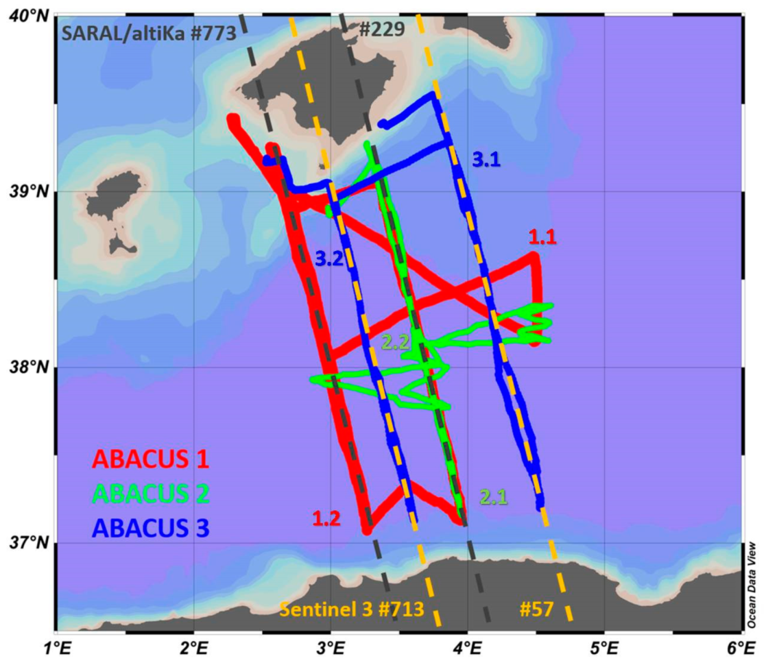
ABACUS glider cruises were developed along a repeated monitoring line across the AB, and allowed the collection of a huge dataset of physical and biological ocean parameters in the first 975 m of the water column. Even though the present study is restricted to a particular area, i.e., the AB, we strongly believe that the scientific community could use our results to enlarge the knowledge of the western Mediterranean Sea and to refine the use of glider missions to validate SMOS SSS products in other regional-scale studies (e.g., those focusing on the Agulhas Leakage, the Malvinas Confluence, the Gulf Stream). BEC SMOS SSS L3 and L4 products, as well as glider measurements and mission strategies, are described in Section 2. Results and discussion are presented in Section 3. Finally, Section 4 reports prominent conclusions.

2. Data and Methods

2.1. Glider In Situ Observations

In 2014, a new repeated monitoring line was created in the western Mediterranean, in the framework of the ABACUS project. Since then, five glider missions have been carried out in the AB from 2014 to 2019, permitting a significant overlap with the satellite SMOS mission and products. In the present work, the glider data collected during the autumns from 2014 to 2016 were used (Figure 1). Additional ABACUS campaigns were developed during fall 2017 and spring 2018 and 2019, but the collected measurements are still under quality control analyses and have not been released yet. Conversely, the ABACUS 2014–2016 dataset was fully quality controlled and is available through a public repository at https://0-dx-doi-org.brum.beds.ac.uk/10.25704/b200-3vf5. This dataset includes a total of eight glider transects realized between the Island of Mallorca and the Algerian Coast to collect temperature, salinity, turbidity, oxygen, and chlorophyll concentration measurements between surface and 975 m depth.

Each mission had an average duration of about 40 days and was always performed in the same season, i.e., between September and December. The timing of the missions was accurately planned in order to provide synoptic in situ observations with respect to the satellite SARAL/AltiKa and Sentinel-3A passages. In 2014 and 2015, after the realization of the defined transects, the glider was deviated from the monitoring line in order to sample specific mesoscale structures identified through near real time satellite altimetry and SST maps (Figure 1).

ABACUS data were collected through Slocum G2 deep gliders diving with an angle of 26° with the sea surface, at an average vertical speed of 0.18 ± 0.02 m/s. The resulting net horizontal velocity is about 0.36 m/s.

The two autonomous platforms used during the ABACUS surveys were equipped with the same instrumentation: a glider-customized CTD by Seabird measuring temperature, salinity (derived from conductivity), and depth; a two-channel combo fluorometer and turbidity sensor by WetLabs; and an oxygen optode to measure absolute oxygen concentration and saturation by AADI. Temperature and salinity were sampled to full diving depth (0–975 m depth). Oxygen data were collected to the same depth, while the acquisition of the other optical parameters ceased at 300 m depth. Physical parameters (temperature and salinity) were sampled at 1/2 Hz, resulting in a vertical resolution of 0.4 m along the water column. CTD details are listed in

Table 1. Sampling rate and vertical resolution of ABACUS gliders’ conductivity-temperature-depth (CTD) sensors (* full scale range).

Parameter	Instrument	Sampling Rate (Hz)	Vertical Resolution (m)	Depth Range (m)	Accuracy	Resolution
Conductivity (C) Temperature (T) Depth (D)	Seabird GPCTD glider payload pumped CTD	1/2	0.4	0 to −975	C: ±0.0003 S/m T: ±0.002 °C D: ±0.1% fsr *	C: 0.00001 S/m T: 0.001 °C D: 0.002% fsr *

. Furthermore, it is important to remark that glider measurements were not precisely at the sea surface; however, they were closer to the ocean–atmosphere interface than Argo can usually achieve. In fact, the shallowest glider observations range between 0.22–0.99 m depth during ABACUS surveys, while Argo floats usually stop pumping water around 2–5 m depth.

Temperature and salinity sensors were regularly calibrated after every glider mission in order to guarantee the quality of the measurements. After each mission, data were transferred from the internal glider memory to the SOCIB Data Center, where data processing was carried out and production of delayed time NetCDF files (i.e., level 1 and level 2) occurred before web dissemination of the data.

In the present study, we make use of the level 2 salinity dataset that includes regularly sampled vertical profiles obtained by interpolation of level 1 data from each up or downcast. Data processing included thermal lag correction, which was applied following a specific procedure developed for gliders [47], filtering, and 1 m bin vertical averaging [48]. Nevertheless, an additional quality control procedure was developed and regularly performed at University of Naples “Parthenope” to identify and discard bad data and artifacts that were still present after the level 2 processing. This procedure included a single-point spike control, an interpolation of single missing data along the profiles, and a five-point running mean along the depth; finally, an iterative comparison between adjacent profiles was performed [17]. As for salinity measurements, the detailed results previously reported [17] confirm that ABACUS glider uncertainties are smaller than the typical values that characterize the AB natural variability at surface layer, and thus are accurate enough to capture and correctly describe the main thermohaline properties of the AB water masses and their variability.

Finally, it is important to remark that during the 2014 surveys, only the downcast samplings were collected, breaking the surface at every 8 km; both downcasts and upcasts were gathered in the mission conducted in 2015 with no changes in surface breaking; in 2016, the glider was programmed to break surface after every profile (4 km), acquiring both upcast and downcast data. These changes in the sampling and navigation strategy improved the data collection in the very surface layer (depth < 20 m), and provided a more suitable dataset for the chased comparison with satellite data. Indeed, spatial resolution of in situ measurements was improved from 4 km to 2 km, and the number of samples collected in the 0–10 m depth layer increased significantly (i.e., from 25 in 2014 to 150 in 2016, for a regular 12 km interval).

2.2. SMOS L3 and L4 Sea Surface Salinity Products

ABACUS in situ observations were compared to co-located L3 and L4 maps of SMOS SSS, recently obtained at the BEC through the methodology developed by Reference [27]. This methodology takes advantage of a combination of the new retrieval debiased non-Bayesian algorithm, DINEOF, and multifractal fusion to retrieve enhanced SSS fields over the North Atlantic Ocean and the Mediterranean Sea.

The debiased non-Bayesian aims to mitigate the systematic biases associated with the SMOS acquisitions. These are the biases that are expected to be constant under the same acquisition conditions (i.e., those associated to the same location, satellite overpass direction, and antenna coordinates). This methodology has been demonstrated to mitigate a large part of the errors produced by land–sea contamination and errors associated to permanent sources of RFI. However, some residual errors associated with intermittent sources of RFI and residual land–sea contamination were still present in the resulting retrievals. Parts of the temporal dependent residual errors have been characterized and corrected using DINEOF decomposition. The empirical orthogonal functions correlated with the temporal dependent residual errors were removed from the SMOS salinity maps. At the end, the resulting L3 maps provided root mean square differences with respect to an Argo salinity of 0.3 (see

Table 2. Main statistics (mean; standard deviation; linear correlation) of daily differences computed between BEC SMOS L3/L4 SSS and ABACUS in situ SSS along the analyzed glider transects.

Mission	Start	End	SMOS L3-ABACUS	std	R-Value	SMOS L4-ABACUS	std	R-Value
ABACUS 1.1	20140913	20141018	−0.17	0.21	0.23	−0.13	0.17	0.39
ABACUS 1.2	20141120	20141215	−0.28	0.17	0.76	−0.24	0.16	0.80
ABACUS 2.1	20151020	20151110	−0.25	0.20	0.52	−0.23	0.22	0.37
ABACUS 2.2	20151111	20151211	−0.22	0.24	0.22	−0.22	0.24	0.25
ABACUS 3.1	20161105	20161130	−0.17	0.14	0.72	−0.11	0.12	0.65
ABACUS 3.2	20161130	20161215	0.13	0.12	0.78	0.19	0.13	0.73

in Reference [27]). After applying both corrections, the spatial distribution of the errors is pretty uniform in the western Mediterranean (see Figure 5 in [27], first plot of the second row). This suggests that the errors associated with land–sea contamination and RFI in the western Mediterranean have been mitigated. Conversely, systematic negative biases still appear in the eastern part of the basin, of which regions appear more degraded due to RFI contamination.

Furthermore, multifractal fusions were applied to BEC SMOS L3 maps in order to increase the spatial and temporal resolution of the SMOS salinity maps. This was done using OSTIA SST maps as a template [49]. The resulting L4 maps showed coherent (and better resolved) spatial structures in some specific regions, as the Alboran Sea and the Gulf of Lion. Due to limitations of the fusion methodology and of the effective spatial resolution of the template, the effect of the fusion method sometimes produces an additional smoothing to the SSS maps, preventing an actual improvement of the effective resolution of the L3 maps. This phenomenon has also been observed during the present study; although several structures are better resolved by L4 products, we did not observed an evident improvement of the effective resolution for all the analyzed SSS maps of the AB.

Nonetheless, these products present an improved accuracy in the Mediterranean basin with respect to the objectively analyzed maps and the L4 products previously available, i.e., a reduction of both the seasonal bias and the standard deviation of the error [27].

In this study, we used L3 nine-day binned maps at 0.25° and L4 daily maps at 0.05°, which are freely available at http://bec.icm.csic.es/ocean-experimental-dataset-mediterranean/. L3 maps are generated by using 9 days of SMOS acquisitions and by applying a scheme of objective analysis. They are generated daily on a grid of 0.25° × 0.25°. L4 maps are generated by fusing the nine-day L3 maps with daily OSTIA SST maps, so that the day of the SST map corresponds to the central day of the SMOS nine-day period. The L4 SMOS SSS maps inherit the resolution of the OSTIA SST maps (0.05° × 0.05°).

The co-location of SMOS and glider SSS was performed comparing the uppermost (0–10 m) SSS measurements provided by the ABACUS gliders at the instant t0, with the SMOS SSS field given by the nine-day map (t0 at 4 days). ABACUS SSS deeper than 10 m were not considered in this study.

2.3. Altimetry and Sea Surface Temperature Maps

In this study, we combined altimetry observations and SST information in order to improve the description of the main features of the western Mediterranean Sea during the analyzed glider surveys. The final goal was to evaluate the presence of filaments and mesoscale structures that could have caused the observed difference between SMOS and glider SSS values.

As for altimetry, we used Mediterranean Sea gridded L4 daily absolute dynamic topography (ADT) and geostrophic currents computed with respect to a twenty year 2012 mean by Optimal Interpolation, merging the measurement from all altimeter missions (i.e., Jason-3, Sentinel-3A, HY-2A, SARAL/AltiKa, Cryosat-2, Jason-2, Jason-1, T/P, ENVISAT, GFO, ERS1/2) through the DUACS multimission altimeter data processing system [50]. To produce reprocessed maps of ADT in delayed-time, this system uses the along-track altimeter missions from products called SEALEVEL*_PHY_L3_REP_OBSERVATIONS_008_*. The datasets are available from the CMEMS web portal (http://marine.copernicus.eu/services-portfolio/access-to-products/).

L4 SST foundation data were provided by the NASA Jet Propulsion Laboratory Physical Oceanography Distributed Active Archive Center (PODAAC). We opted for MUR-SST foundation products (full name JPL-L4_GHRSSTSSTfnd-MUR-GLOB-v02.0-fv04.1) that spanned from June 2002 to the present [51]. The dataset is available at ftp://podaac-ftp.jpl.nasa.gov/allData/ghrsst/data/L4/GLOB/JPL/MUR as a netCDF file containing daily global SST data at a spatial resolution of 0.01° in longitude–latitude coordinates (about 1 km intervals). These maps are made mostly from satellite SST measurements, with help from surface observations from ships and buoys. Ultra-high resolution is achieved for the MUR-SST foundation dataset through the application of a multi-resolution variational analysis. In general, this dataset compares well in magnitude and phase with the lower resolution products (e.g., OSTIA); it also allows identification of interesting finer scale structures that are most likely due to meso- and submesoscale eddies.

3. Results and Discussion

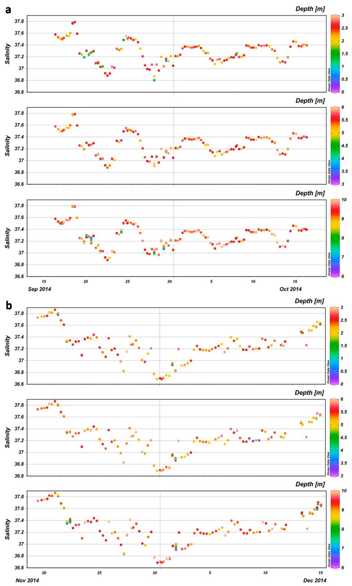
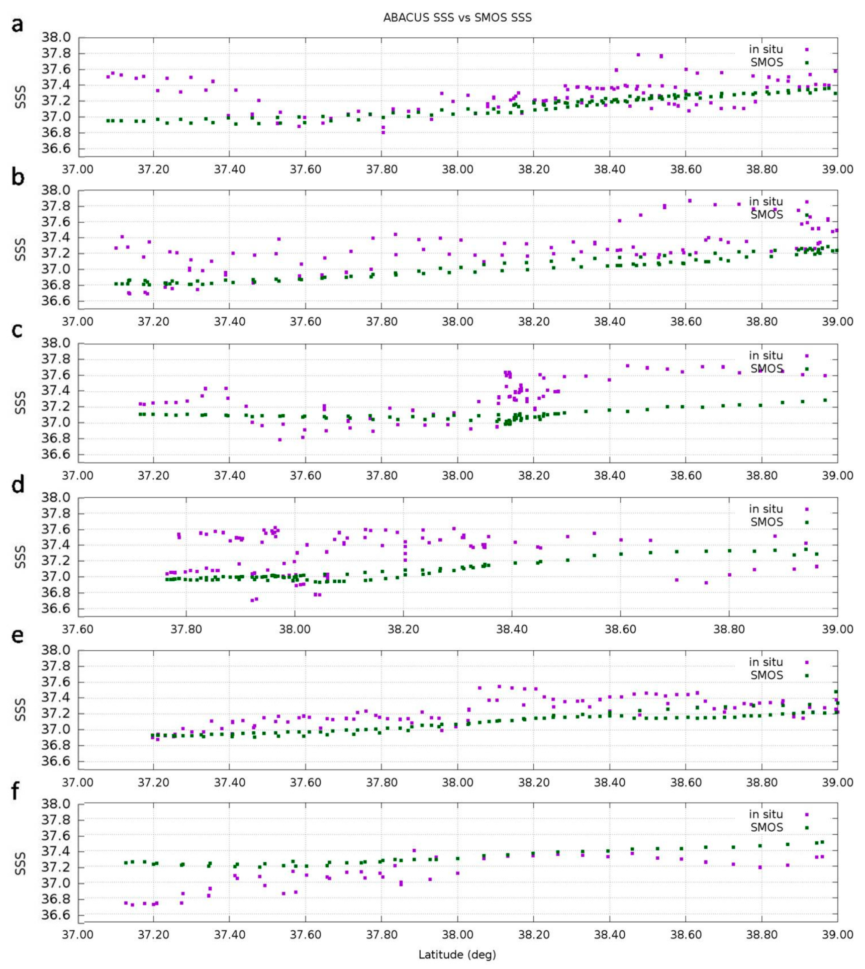
We compared SMOS SSS, which represents few centimeters of depth, and the corresponding integrated value of the pixel area, with the mean salinity value provided by the first 10m depth of ABACUS observations. This subset was chosen according to the analysis of SSS values measured by ABACUS glider. To this aim, observations collected in the first 10 m depth were divided into three bands, i.e., 0–3 m, 3–6 m, and 6–10 m depth. The example reported in Figure 2 shows that SSS did not present a significant variability with depth in this very surface layer during the ABACUS 1 glider surveys; this result reflects the thermocline location at depths greater than 10 m during these cruises [17]. Similar results were obtained for the ABACUS 2 and ABACUS 3 observations.

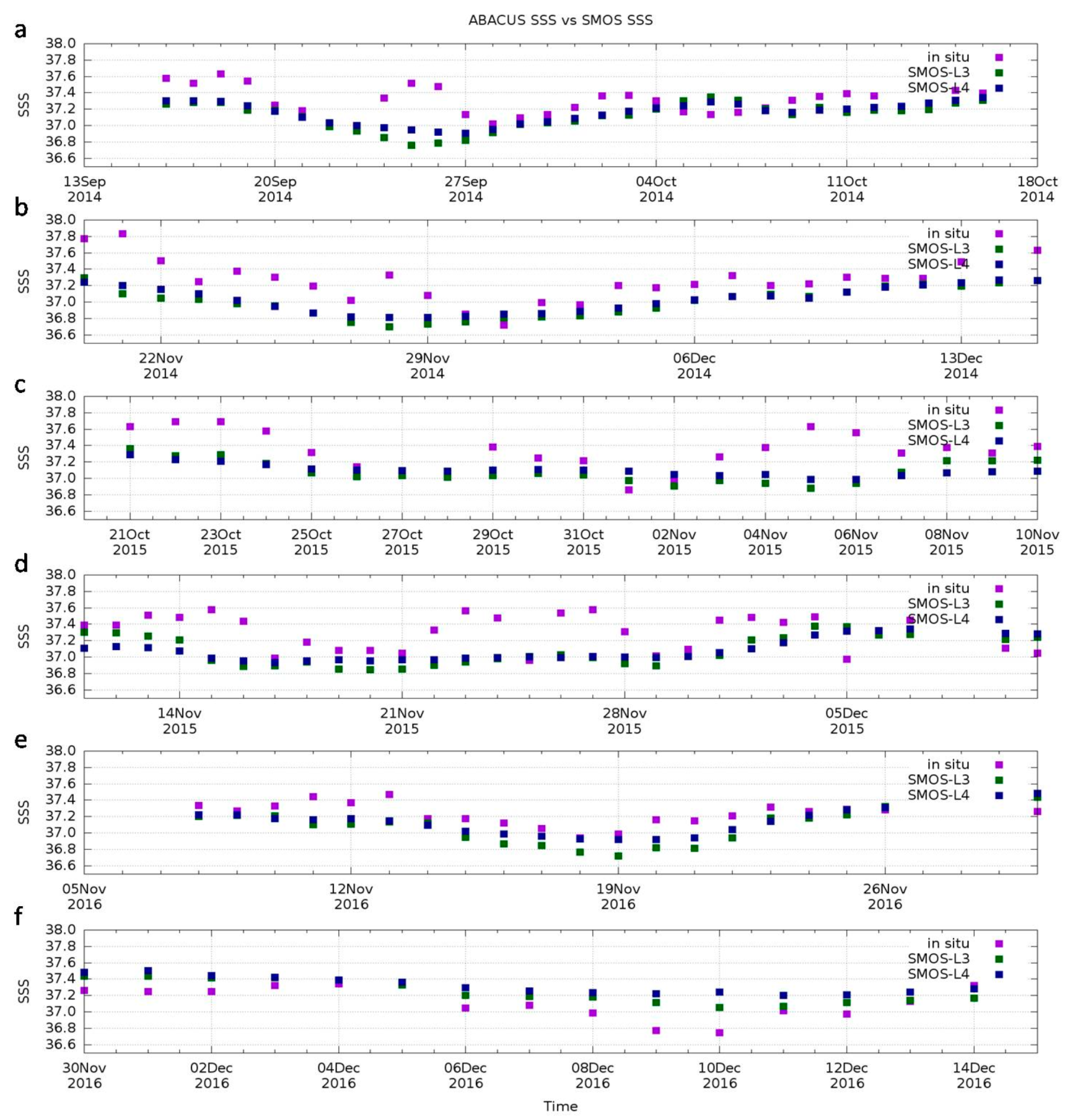
We then spatially averaged the ABACUS salinity of the 0–3 m layer in the same pixel of SMOS. The resulting averaged value was compared with SMOS L3 and L4 maps available for different dates (Figure 3).

3.1. Overall Results

In spite of the limitation associated with the differences in the spatial and temporal resolutions, the enhanced SMOS products represent well the salinity patterns described by in situ SSS, although slightly underestimating ABACUS observations. Over 6799 comparisons, a mean difference of −0.14 was estimated between SMOS L3 and ABACUS SSS, the standard deviation of difference (std) being 0.25. The achieved results are similar to those previously estimated by Argo floats (−0.16, with a std of 0.34) [27], and fall within the range of variability that typically characterizes AB surface salinities during the September–December season [17]. The very small uncertainties associated with the glider measurements do not seem to appreciably condition these statistics.

Figure 3 shows that SMOS L3 retrievals represent well the qualitative evolution of surface salinity along the glider transects. Nevertheless, SMOS estimations were still far to be coincident with in situ high resolution measurements, and their smoothed behavior prevented them reproducing local variability, possibly due to submesoscale structures, lenses, and other small scale phenomena intercepted by gliders and recorded in the in situ dataset. In this sense, the main statistics of the analyzed ABACUS surveys, reported in Table 2, suggest that SMOS L3 retrieval capability can vary largely across different glider experiments, depending on local dynamics and ocean structures.

Similar results were achieved from the comparison with SMOS L4 products that returned a mean difference (SMOS-ABACUS) of −0.11 and a std of 0.26; linear correlation among satellite and in situ datasets (R-values in Table 2) was not improved significantly by L4 products, except during the ABACUS 1 survey. This suggests that specific features captured by in situ observations are not resolved by SMOS products, even the L4 one.

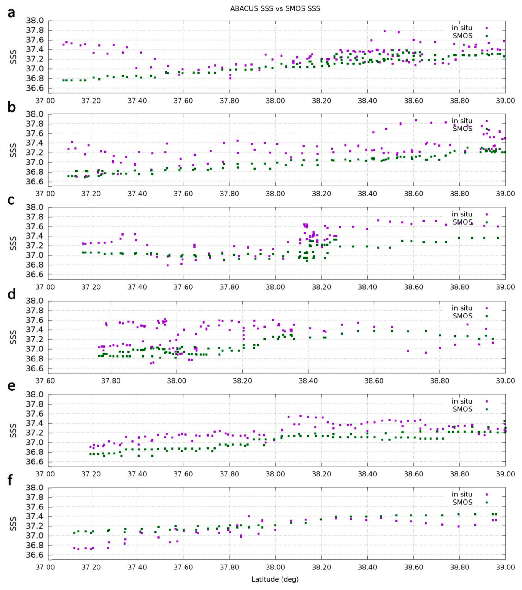
However, the advantages of the downscaling algorithm used for producing L4 products emerge when looking at the latitudinal comparisons between ABACUS and SMOS products. Figure 4 and Figure 5 show that L4 SSS are generally saltier than L3, thus being typically closer to in situ SSS measurements. This is more evident at lower latitudes, i.e., between 37.1 and 37.5° N, where SMOS L4 SSS are saltier than L3 by a factor of up to 0.2. On the other hand, L4 estimations can be smoother than L3, thus a lower correspondence to glider observation was found in other sub-regions of the study area, i.e., between 38.2 and 38.6° N, where L3 products manage to capture part of the finer scale phenomena that L4 products are not able to describe.

In general, we can assess that, for the most of the co-locations, SMOS measured fresher SSS than the in situ, with larger discrepancies at the edges than in the middle of the transects. Nevertheless, some positive differences (SMOS saltier than in situ) were observed locally (i.e., in proximity of the AC during the December 2016 cruise and in short segments of the other transects), although usually lower in absolute value than those typically observed in case of fresher SMOS SSS anomalies.

The largest differences were located at the northern and southern edges of the transects during the four glider surveys carried out in September/October 2014 (Figure 4a and Figure 5a), November/December 2014 (Figure 4b and Figure 5b), October/November 2015 (Figure 4c and Figure 5c), and December 2016 (Figure 4e and Figure 5e). This could suggest that differences are due to some kind of residual land–sea contamination or non-permanent RFI in the satellite data. However, during November 2016 (Figure 4d and Figure 5d), the maximum differences were not in the edges but in the latitude range of 38.0–38.2° N, that is, in the middle of the AB, and too far from the coast.

Although we were conscious that several studies (e.g., References [26,52]) previously demonstrated that interpolated SMOS SSS fields are able to resolve intense mesoscale structures that generally coincide with those identified by gliders and described by altimetry and MODIS images [7,12], we tried to correlate the ABACUS-SMOS differences that came to light with the presence of oceanographic mesoscale events that the fine spatial–temporal resolution of the glider is able to capture but the satellite probably cannot. This was intended to identify a possible origin of the increase of the error in the observed sub-regions. To this aim, we analyzed satellite SST and altimetry maps over the study area in order to evaluate: (i) the presence of interesting mesoscale structures; and (ii) the eventual interactions with peculiar water masses, in particular at the very active northern and southern edges of the ABACUS transects which are characterized by the proximity of the Mallorca Channel and the AC, respectively.

As supposed, our results show that lower correlation values coincide with transects (i.e., ABACUS 1.1, ABACUS 2.1, and ABACUS 2.2) characterized by zone of sharp salinity changes due to intense mesoscale activity and AC meandering. Hence, we conclude that BEC SMOS products capture well the broad resolution of the salinity pattern, but cannot properly resolve the finer scale variability that needs higher resolution to be detected. Several case studies from the analyzed ABACUS surveys are discussed in detail in the following subsections.

3.2. ABACUS 1 Surveys

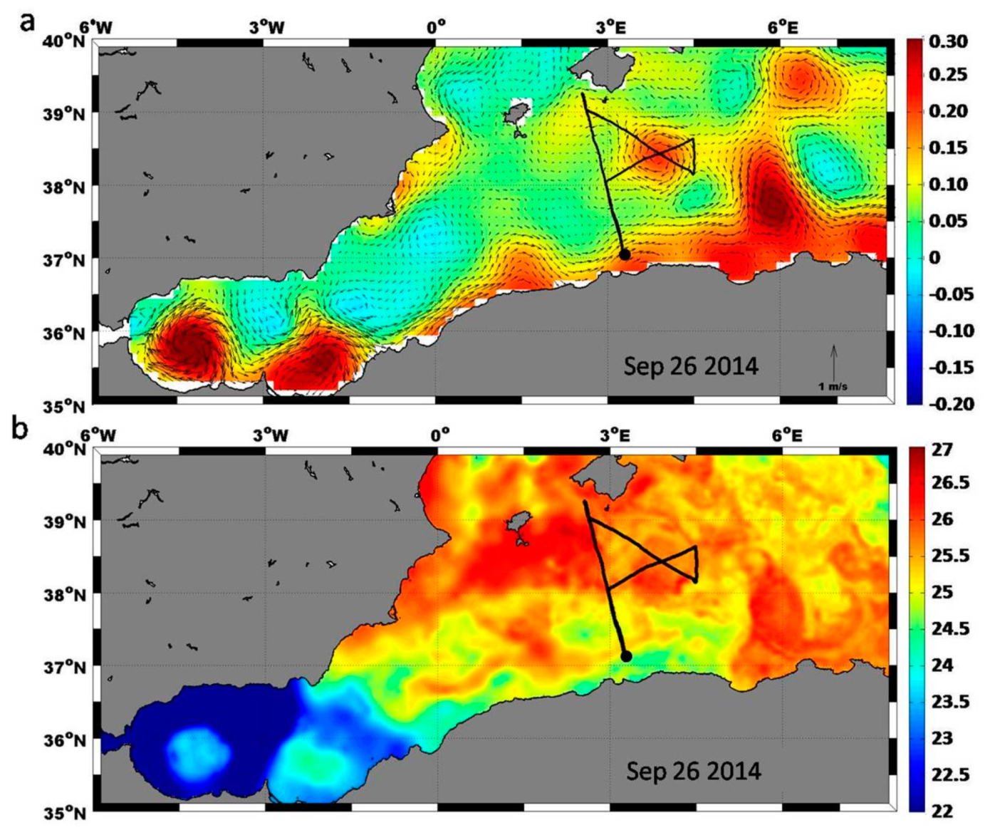
During the ABACUS experiment carried out in September–October 2014, the most significant difference between in situ and SMOS SSS was detected at the southern edge of the glider transect, i.e., between 37.1 and 37.5°N (Figure 4a and Figure 5a). The glider crossed this region between 24 and 27 September (Figure 3a); the transect’s southernmost waypoint was hit on 25 Sept (at 23:47 UTC). This means that the largest differences were estimated when the glider was navigating across the border of the AC influence zone. This area is typically characterized by large instabilities in the surface layer, with meandering activity that allows AW transported by AC to intrude into the more homogenous resident surface water of the AB. At the time of SMOS-glider co-location on 26 September (Figure 6), for example, an intrusion of fresher AW coming from the AC was present in the 0–200m depth section of the water column (see Figure 10a in Reference [7]), but could not reach the surface due to the presence of a local cap of saltier water (up to 37.55). Since SMOS products are strongly influenced by the presence of the fresher AC, which characterizes the area at large scale, they seem unable to capture the local variability associated with the meandering instability. The downscaling provided in SMOS L4 maps improves the capability to identify finer scale features, but cannot completely resolve them.

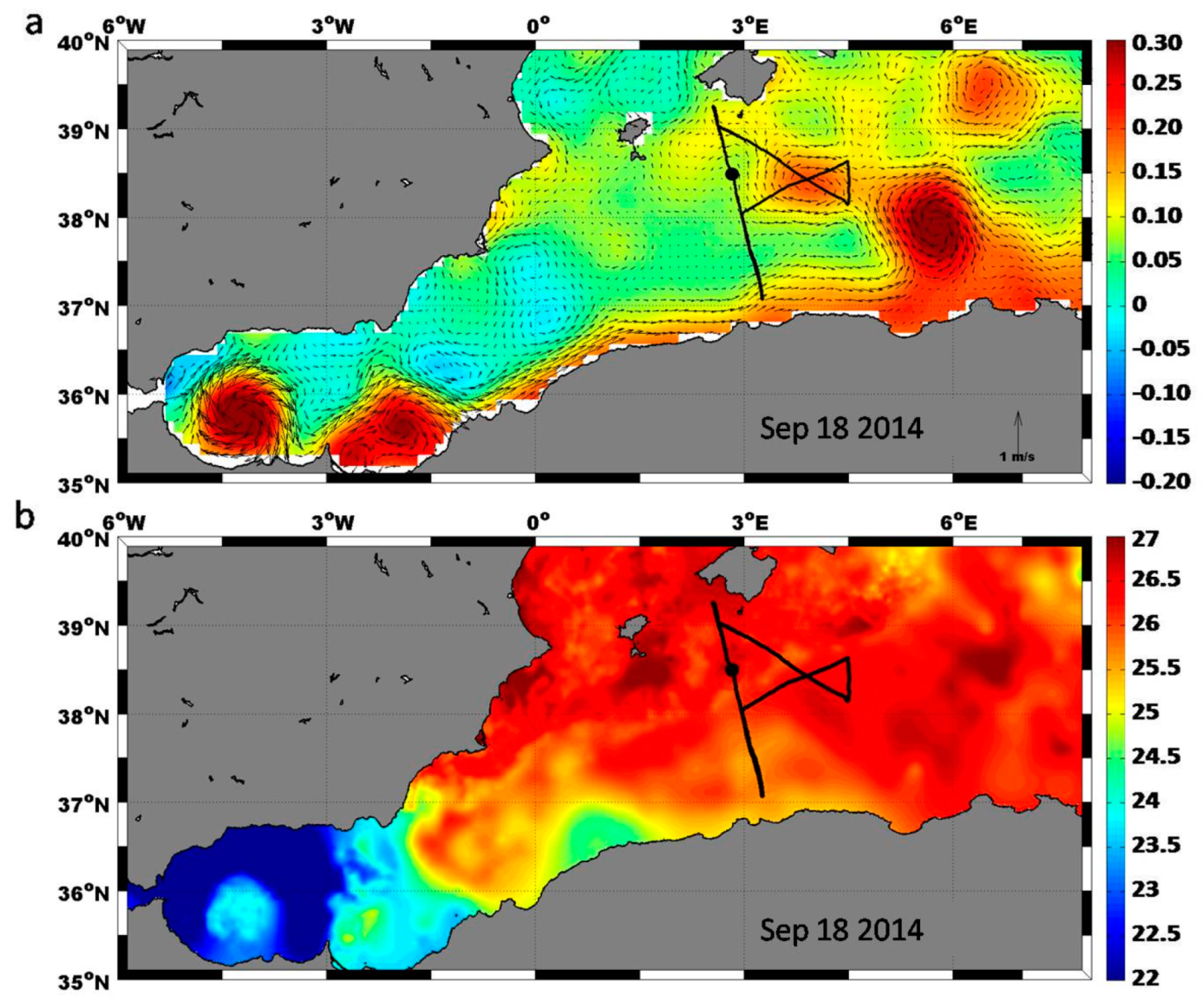
Another significant difference can be found at the beginning of the ABACUS 1.1 survey, when the glider was crossing the area included between 38.4 and 38.6°N on its way south from Mallorca to the AC. In situ SSS showed a rapid and intense increase (up to 0.5 in very few kilometers), with single salinity values up to 37.79 on 19 September, that SMOS L3 and L4 products could not identify (Figure 3, Figure 4 and Figure 5, subplots a). The glider was enough far from the coast to prevent any impact of land contamination, so the observed sudden increase of salinity could indeed be due to the presence of the anticyclonic eddy centered at 2.21°E 38.61°N crossed by the ABACUS glider along its eastern edge (Figure 7).

The region included between 38.4 and 38.8°N is typically characterized by a meandering salinity front in the upper layers which dominates the density distribution, often associated with water salinity asymmetry at the northeastern (saltier) and the southeastern (fresher) edges of the region [53]. A previous study [12] focusing on the mesoscale structure located on the eastern side of the glider transect, and centered at 38.34°N 3.83°E on 18 September (Figure 6 and Figure 7), showed that this eddy was typically characterized by shoaling of isolines on its borders for all the physical parameters, as well as for chlorophyll concentration. They also computed vertical velocities across the eddy to demonstrate the presence of positive (upward) velocities on its southeastern border, thus suggesting that this mechanism may upwell sub-surface and intermediate water (and associated nutrients) to the photic layer.

Thus, we suggest that the spotty saltier in situ values (37.47–37.79) collected on 16–19 September could represent the signature of upwelled saltier sub-surface waters which were intercepted by the ABACUS glider when navigating across the eastern border of the small eddy centered at 2.21°E 38.61°N.

Although SMOS L3 and L4 products retrieve slightly higher SSS in this region in comparison to the rest of the central part of the Mallorca–AC transect, they cannot identify the maximum values observed by the glider, confirming their limits in describing the small scale variability which characterizes the areas of intense local activity. SMOS L4 SSS maps of the Alboran Sea and the AB on 18 September and 26 September 2014 (Figure 8) provide an illuminating example of their scale limitations.

On the other hand, SMOS SSS retrievals correspond well with in situ measurements during the “butterfly shaped” monitoring (2–12October) of the mesoscale anticyclonic eddy located at the eastern side of the ABACUS main transect, which detached from the AC and was centered at 38.34°N 3.83°E on 18 September (Figure 6 and Figure 7). As usual, SMOS SSS were generally slightly fresher than those measured in situ, but they were saltier when the glider was crossing the northeastern region of the monitored eddy (4–7 October).

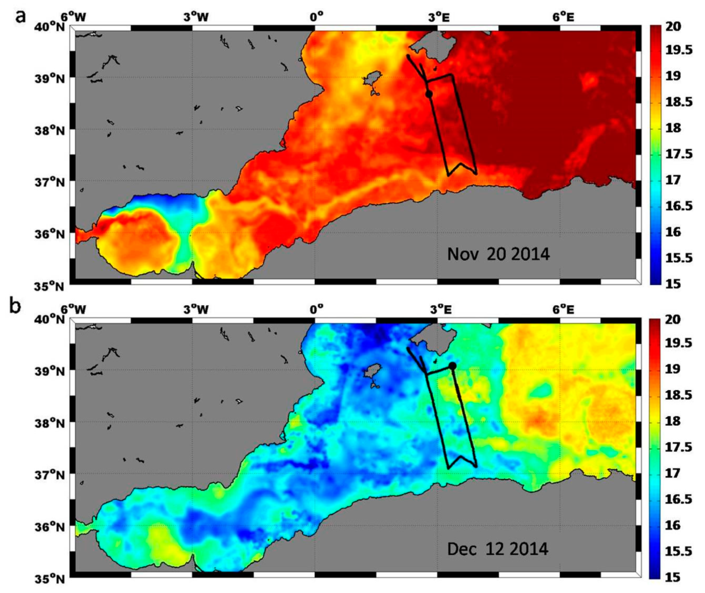
Similar results were achieved for the ABACUS 1.2 experiment, with significant differences between in situ and SMOS SSS identified at the very beginning of the survey (i.e., between 38.4 and 39.0°N), when the glider was diving southward from Mallorca to the AC (Figure 4b and Figure 5b), and close to its southern edge (i.e., between 37.1 and 37.5°N), when the glider entered the region influenced by the proximity of the AC. Smaller but significant differences were also found in the central part of the glider transect (i.e., between 37.7 and 38.0°N).

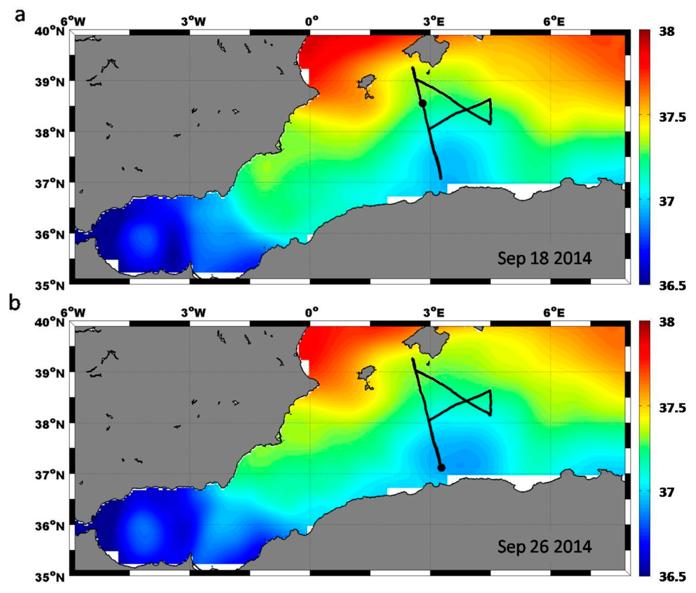
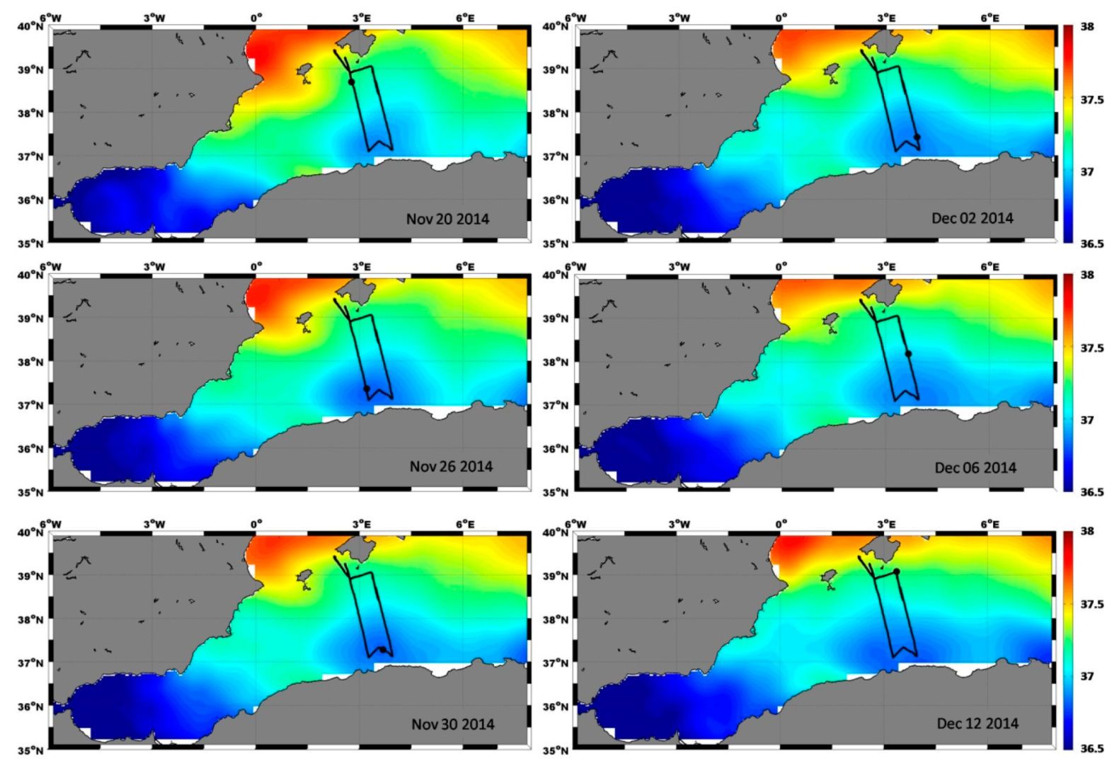
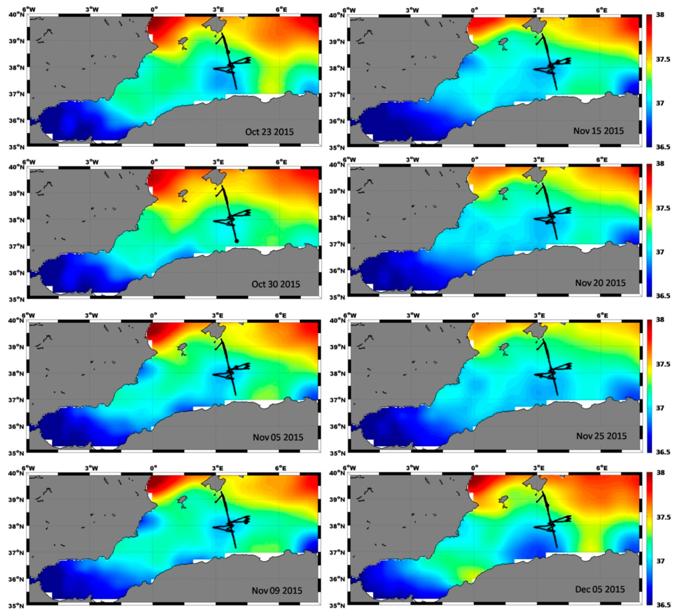
The SST maps of the AB at the beginning/end of this survey (Figure 9) present the peculiar features of this sub-region during the fall season, pointing out the presence of the colder AC flow. Over its area of influence, the SMOS SSS values remain in the middle of those collected by the two passes of the glider, which registered fresher and saltier salinities during its southward and northward passages, respectively (Figure 4b and Figure 5b). SMOS captured the general salinity pattern, but missed the finer scale variability observed in situ. On the other hand, a very good agreement between glider and satellite SSS can be observed during the second part of this experiment (1–12 December) when the glider navigated northward along the easternmost SARAL-AltiKa #229 groundtrack.

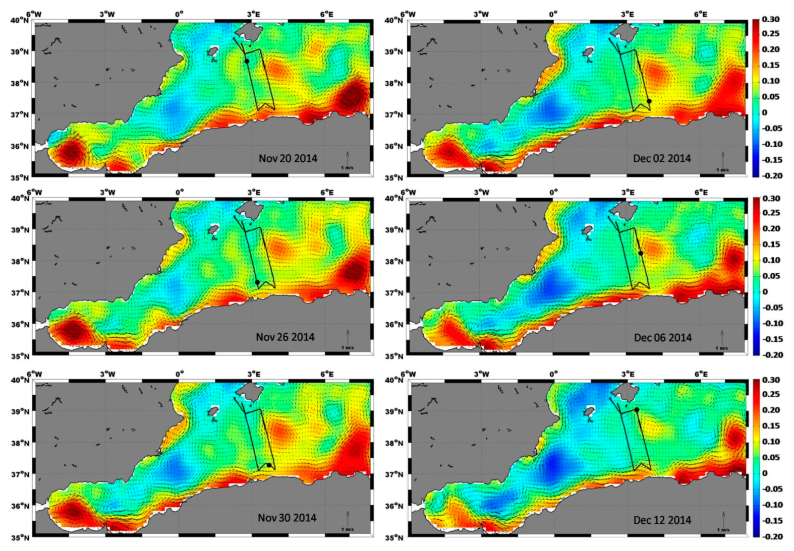
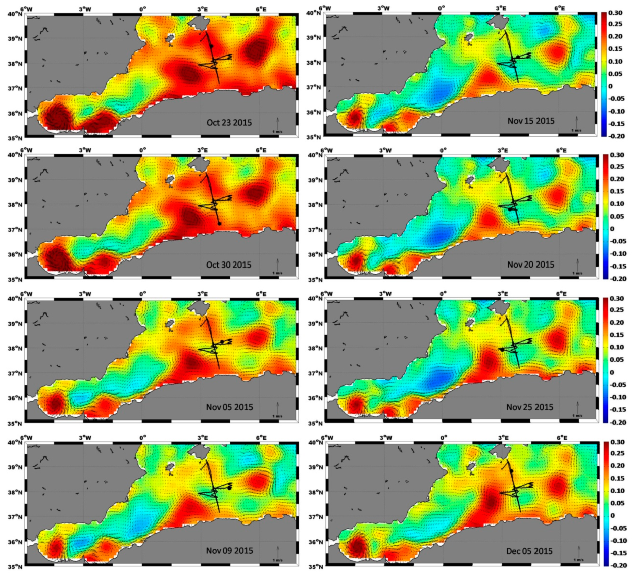
These results are consistent with the observed dynamics of the AB (Figure 10), showing that the glider crossed (i) an area of very intense ocean instability, characterized by the presence of two small cyclonic structures, on its way south; (ii) a much more homogeneous region, delimited and controlled by an intense long-living anticyclonic eddy, on its way north.

The local variability measured when hitting the mesoscale structures in Figure 10 was always associated with a lower correspondence of SMOS SSS retrievals; this happened on 20 and 26 November, when the glider was crossing two small cyclonic eddies, and on 6 December, when it was lining the western border of a large anticyclonic eddy. SMOS limitations to retrieve finer scale reliable SSS are evident in Figure 11.

3.3. ABACUS 2 Surveys

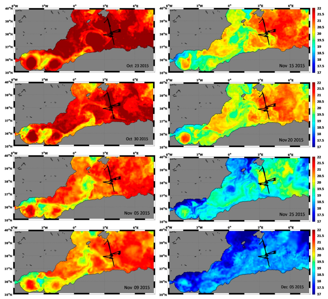
As in ABACUS 1, an evident fresh SMOS anomaly was found in the northern part of the ABACUS 2 transect, i.e., between 38.1 and 39.0°N (Figure 4c), during the glider southward survey from 21 to 23 October 2015 (Figure 3c). This impressive anomaly was not present during the second glider passage at the end of the ABACUS 2 mission, when satellite and in situ measurements correspond much more. Nevertheless, it is interesting to observe that on 5–6 December 2015 (Figure 3d) SMOS SSS looked saltier than those measured in situ in the northern sector of the transect, i.e., between 38.7 and 39.0°N (Figure 4d). As usual, these differences were attenuated in L4 products (Figure 3c,d and Figure 5c,d).

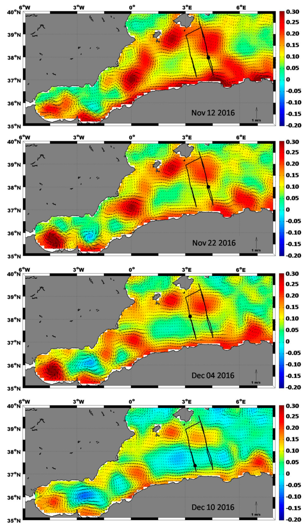
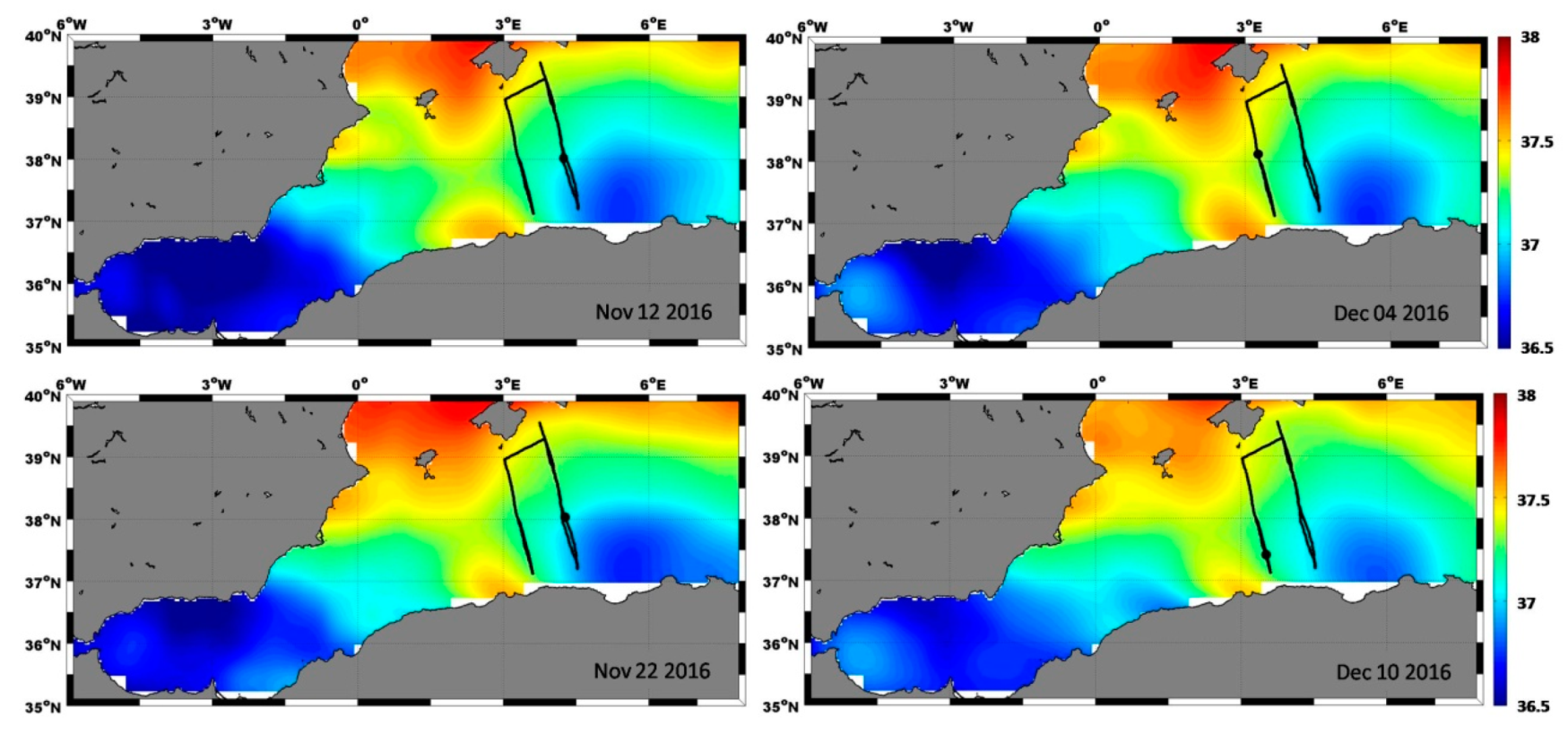
SST conditions (Figure 12) and ocean circulation features (Figure 13) over the AB during the southward and northward transects suggest that the observed differences between SMOS and in situ salinity values could be ascribed to the presence of an intense mesoscale circulation south of the Mallorca Island, which was passed through by the ABACUS glider during its southward transect along the SARAL-AltiKa groundtrack #229 (Figure 1). In fact, during the first week of this survey, the glider crossed the western border of a small but intense anticyclonic eddy moving westward (Figure 13). This eddy was not present anymore at the end of this survey in late November–early December, so that satellite and in situ observations agree better.

As for the salty SMOS anomaly on 5–6 December, it was completely due to an abrupt decrease in the in situ salinities. The available SST and SSH images do not provide any clear explanation of this observation, except the fact that, on this date, the glider met a filament of warmer sea water that patched the area south of Mallorca during late autumn 2015 (Figure 12). This filament would have been out of the spatial scales resolved by SMOS satellite (Figure 14).

SMOS L3 SSS values were generally fresher than in situ ones also in the latitude range 37.1–37.5°N, i.e., in proximity of the area of influence of the AC border (Figure 4c). As in 2014, this anomaly was reduced but still present in L4 products (Figure 5c). The glider went through this area between 28 and 31 October 2015, and hit waypoint south on 30 October. Figure 12 highlights the presence of a colder filament characterized by a SST of about 20°C in this area, which was crossed by the ABACUS glider at the latitude of approximately 37.4°N; its presence was revealed by in situ measurements, but not by SMOS retrievals (Figure 4c and Figure 5c).

Figure 5c points out also the issue of different temporal scales between satellite and in situ observations. The ABACUS glider covered the transect section in the latitude range 37.7–38.1°N twice at a short temporal distance. During its way southward (24–27 October), it measured fresher SSS, while saltier values were observed on its way back northward (15 November). Despite the short temporal distance, salinity can differ up to 0.4. SMOS SSS retrievals over this latitude sector presented intermediate values between the two passages; again, the general feature was well described, but local short-time variability was not captured.

Significant SMOS fresh anomalies were also recognizable in the center of the AB during the second half of November, when the glider carried out a sort of butterfly monitoring activity on the two sides of the main SARAL-AltiKa groundtrack. On the eastern side, the glider reached and monitored (9–12 November) the border of an anticyclonic eddy moving away eastwards (Figure 13); SMOS maps seem to capture well part of the local variability as observed in situ (Figure 3d). On the western side, a cyclonic eddy was entirely crossed by the ABACUS glider (22–30 November) up to its border region, with another anticyclonic structure (hit on 26 November) detaching from the AC (Figure 13). Although the general salinity pattern was captured (Figure 14), in this case, both L3 and L4 SMOS SSS largely underestimated glider measurements (Figure 3d).

3.4. ABACUS 3 Surveys

During fall 2016, both L3 and L4 SMOS retrievals were slightly fresher, but in very good agreement with in situ measurements (Figure 3e,f). This could also have been favored by the improved resolution in glider surface acquisitions during this survey.

Nonetheless, the latitudinal comparison pointed out some fresh SMOS anomalies between 38.0 and 38.2°N, during the glider dives along the Sentinel 3 satellite groundtrack #57 (hereafter ABACUS 3.1 cruise). The glider covered this sector twice during ABACUS 3.1, first on 11–13 November (southward leg), and then on 21–23 November (northward leg). These fresh SMOS anomalies were smaller than those observed in the previous campaigns, and disappeared during the following glider passages at the same latitude (December 2016), along the Sentinel groundtrack#713.

The AVISO SSH maps in Figure 15 show that a similar circulation pattern persisted over the AB during both the southward and the northward legs along the Sentinel groundtrack #57 (November 2016). This eastern transect was completely dominated by the presence of an intense anticyclonic eddy that the glider went through, along its north–south axis, during both passages. This mesoscale structure was much more intense during the southward leg; this could explain the moderate fresh anomalies observed in SMOS SSS on 11–13 November.

Conversely, SMOS retrievals could not capture the evident SSS decrease measured by the glider along its western transect (hereafter ABACUS 3.2). In particular, salty SMOS anomalies, unexpectedly accentuated in L4 products, were identified along most of its northward leg, i.e., between 6 and 12 December 2016 (Figure 3f). As for the rest of ABACUS 3.2, satellite and in situ measurements agree very well. Figure 15 suggests that the observed differences could be due to the presence of an intense cyclonic mesoscale structure developing in the southern sector of this transect, the western boundary of which was crossed by the glider from 6 to 12 December 2016. On these dates, SMOS L4 SSS maps did not capture any evident salinity decrease associated with the presence of this mesoscale structure (Figure 16).

4. Conclusions

The comparison with the ABACUS in situ measurements shows that, in spite of the limitation of the differences associated with the spatial and temporal resolutions, the analyzed BEC enhanced SMOS SSS products provide a coherent description of the salinity patterns in the AB. This supports the results previously reported [27], which demonstrated that the statistical filtering criteria, the EOF decomposition, and the debiased non-Bayesian retrieval-DINEOF-fusion approach behind the L3 and L4 products improve the salinity retrievals with respect to official SMOS Level 2 Ocean Salinity products.

SMOS retrieved L3 and L4 SSS values were generally slightly fresher (approximately −0.11, −0.14) than those collected in situ, which also captured more salinity variations, including those usually associated with local variability. Larger fresh SMOS anomalies emerged in proximity of dynamic mesoscale structures, i.e., in the area of influence of the AC and/or in presence of intense cyclonic and anticyclonic eddies. Only a few cases showed salty SMOS anomalies, e.g., when observing an area characterized by the presence of an intense cyclonic eddy during the ABACUS 3.2 survey.

As expected, the BEC L4 corrected products generally improved satellite retrievals, reducing differences with in situ measurements when a fresh SMOS anomaly was observed. However, the effective resolution of the L4 SMOS products still cannot capture all the small scale structures that in situ data do.

These results suggest that (i) SMOS retrievals are able to describe well the large scale salinity patterns in the AB; (ii) the existing differences are associated with neither systematic biases nor land contamination, but depend on the actual satellite capability of resolving local variability due to intense and rapidly evolving mesoscale dynamics.

On one hand, although the native resolution of the satellite is about 45 km, the effective resolution of the L3 product is driven by the correlation radii used in its generation (175, 125, and 75 km). These radii are too large for describing parts of the mesoscale dynamics of this region. On the other hand, the results obtained from the L4 products indicate that the simplified scheme of multifractal fusion (scalar approach [30]) is not enough to fully describe the fast, small-scale dynamics present in this region, and that more complex schemes are needed (such as the vector approach [30] that was used in Reference [26] for capturing eddies in AB). Therefore, since the large scale salinity patterns are well described, future releases of these products should now be focused on using different interpolation/fusion schemes to improve the effective spatial and temporal resolutions of the SMOS SSS products. Since systematic negative biases still appear in the eastern Mediterranean Sea, a better mitigation of RFI contamination will then be required in these regions, for example by improving the quality of the brightness temperature with methodologies [54,55] that have already been proven to improve salinity retrieval in coastal areas [56]. Furthermore, all the ABACUS high resolution in situ data used in this study come from three glider surveys carried out in the AB during fall season (i.e., September to December). Additional efforts should set up BEC SMOS L3 and L4 products for evaluation during the rest of the year. To this aim, since 2018, new research efforts have been invested by present authors to realize additional ABACUS glider experiments in the AB during springtime (e.g., ABACUS 4.2 was carried out in May 2018). An analysis at the seasonal scale might also improve the comparison in this region and extend the application of a similar approach in other Mediterranean regions, also favoring the investigation and test of the future releases of the SMOS and the other missions (e.g., NASA Soil Moisture Active Passive—SMAP) SSS products.