Determining the Boundary and Probability of Surface Urban Heat Island Footprint Based on a Logistic Model

 , ,
, ,
Abstract
:1. Introduction
2. Materials and Methods
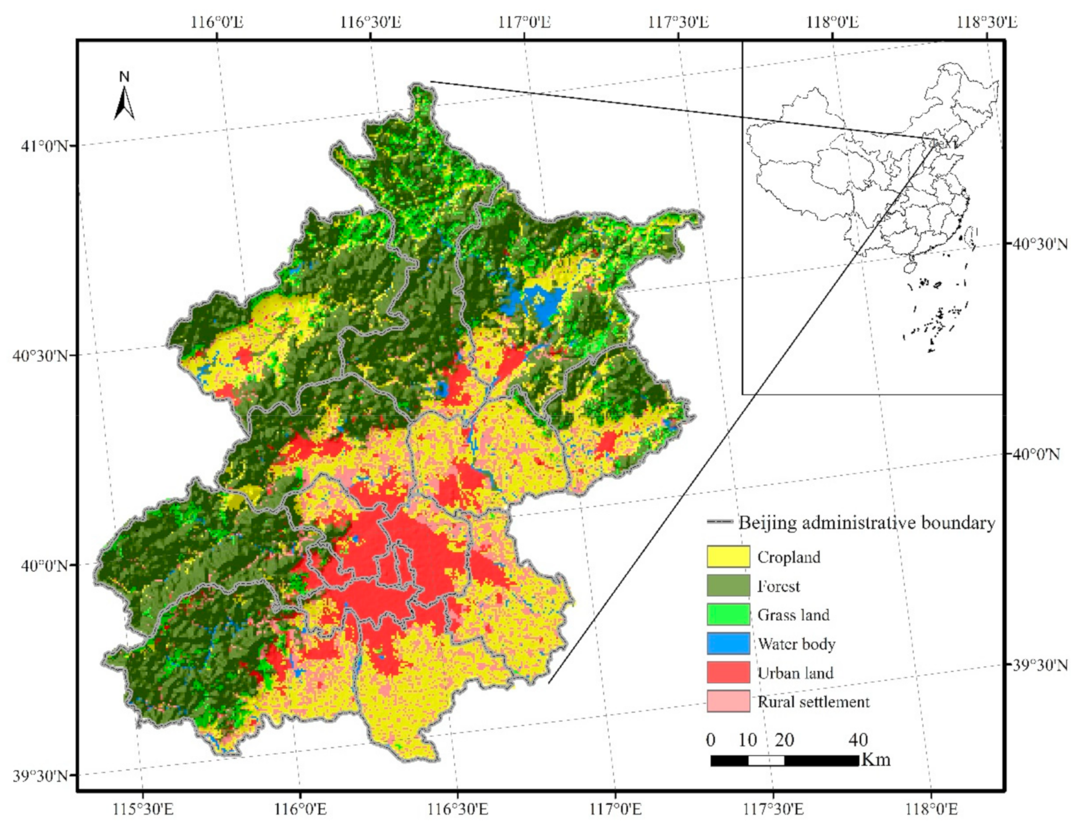
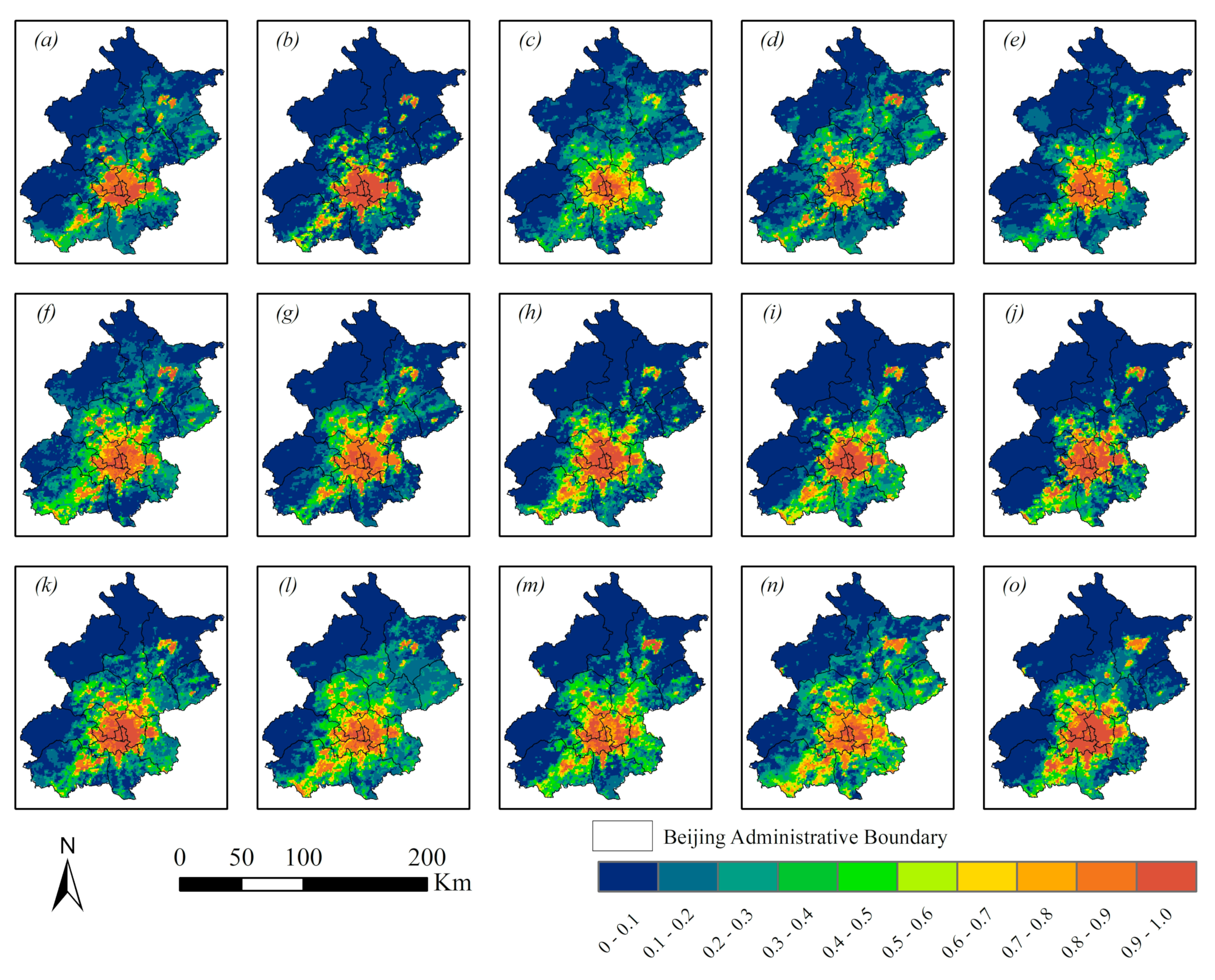
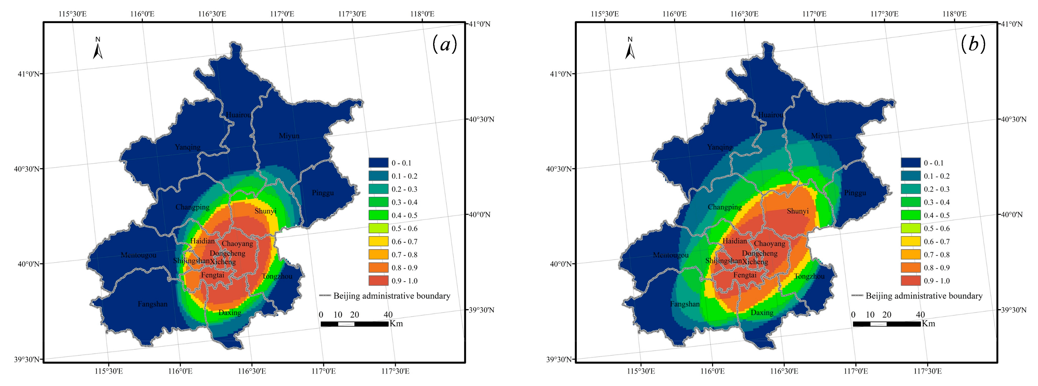
2.1. Study Area
2.2. Data Source
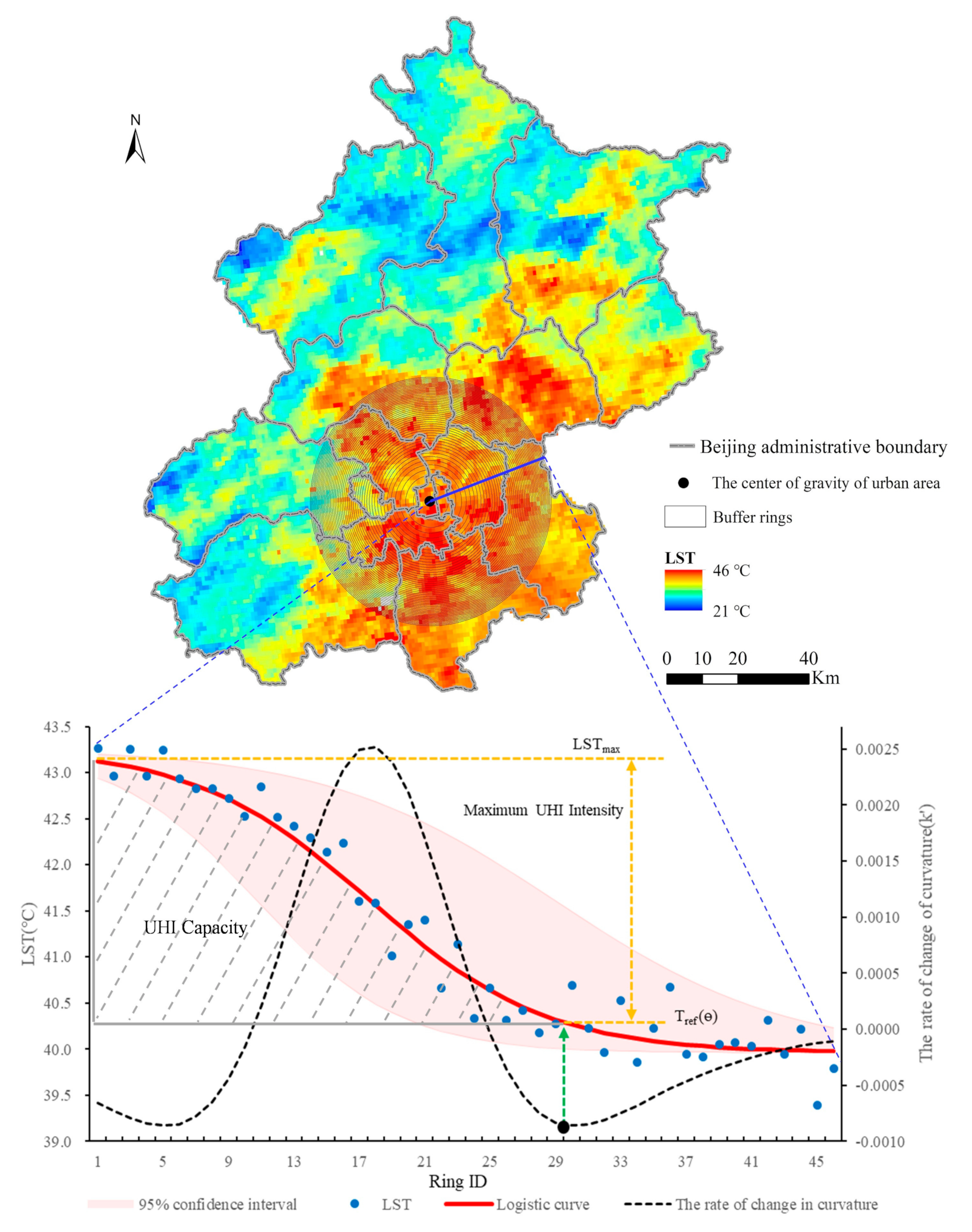
2.3. Method
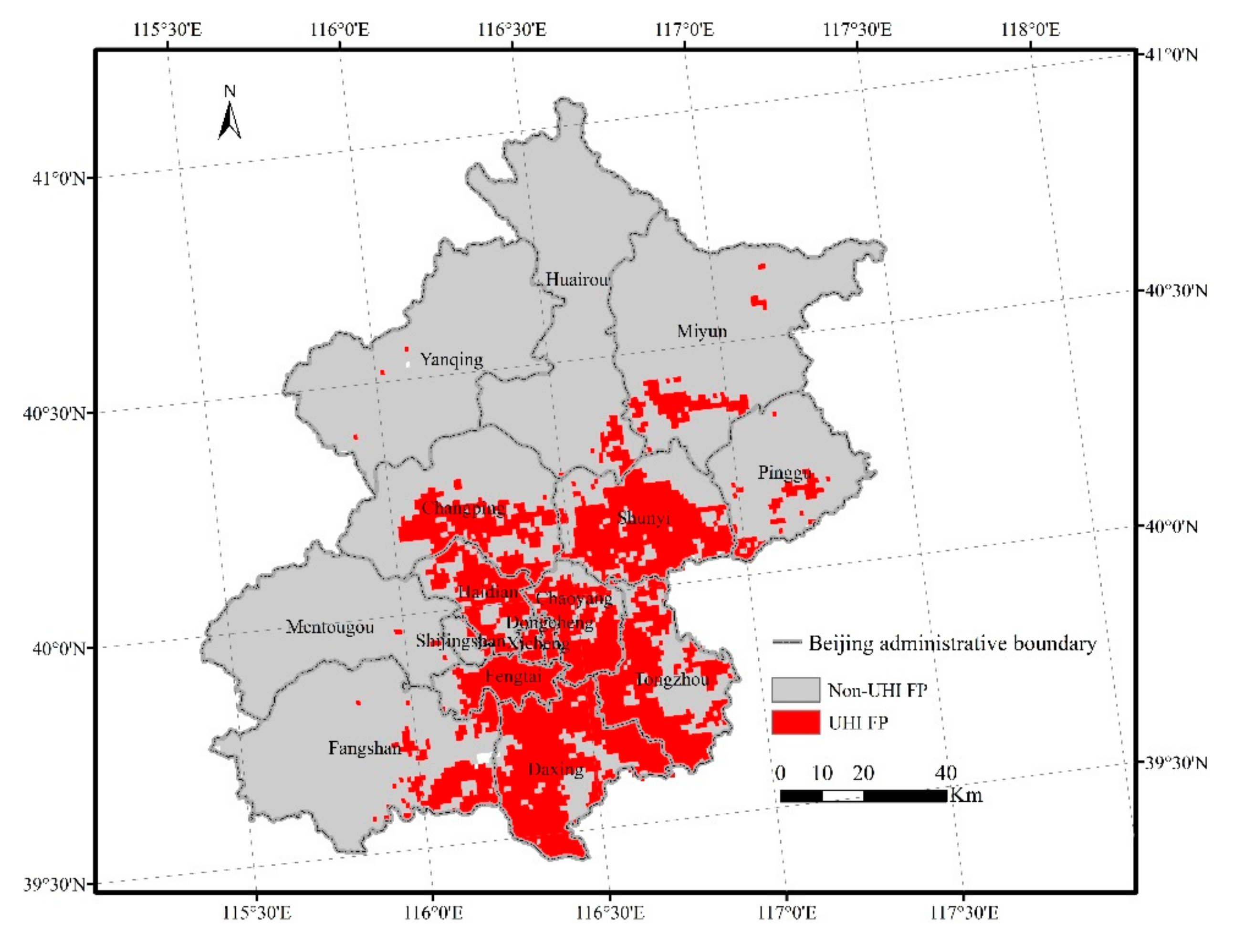
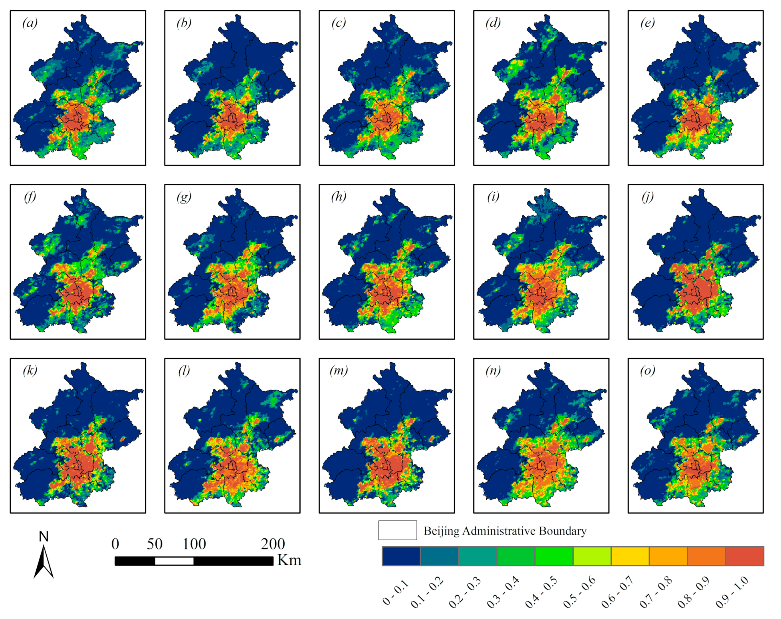
3. Results
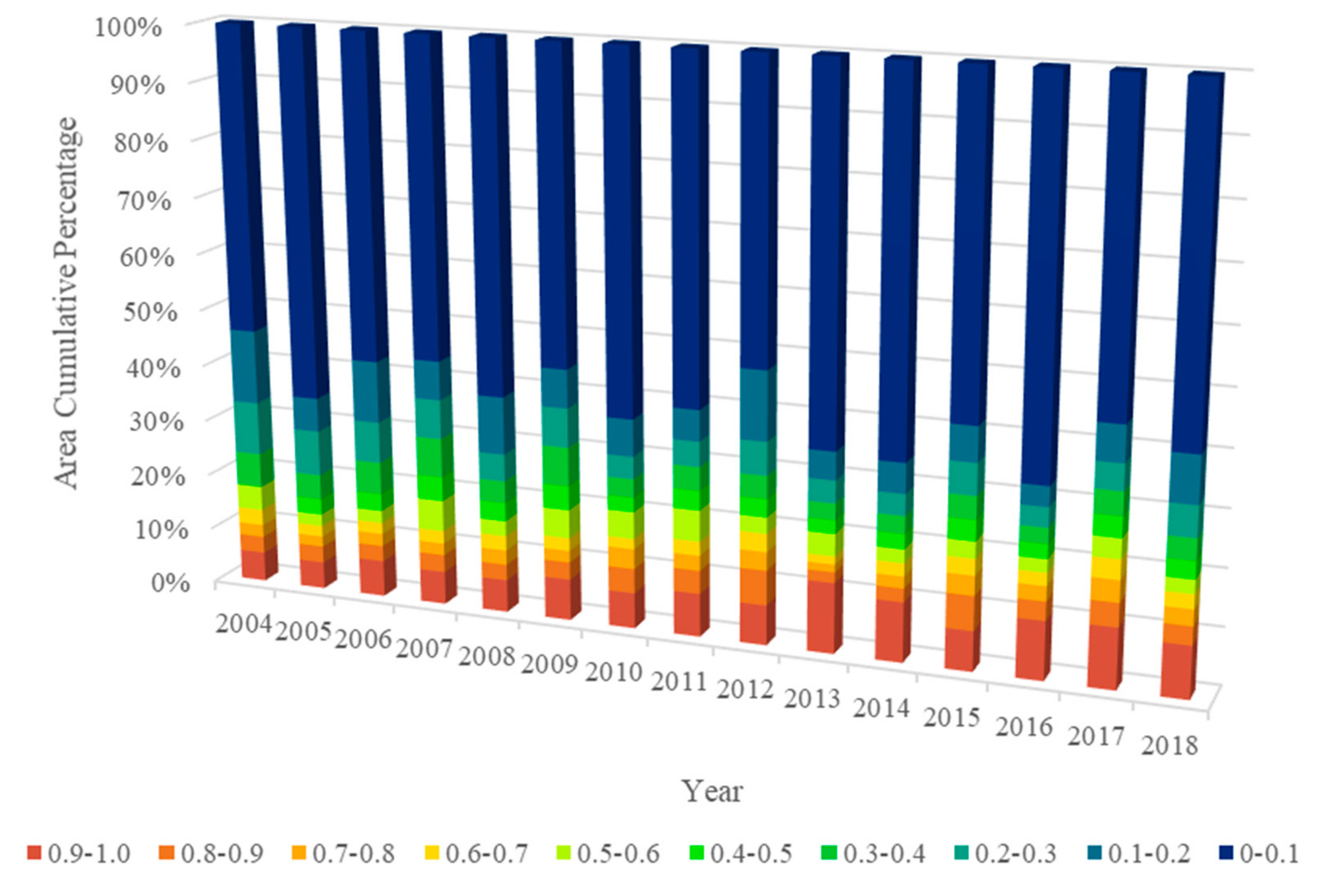
3.1. Spatiotemporal Variation in the FP
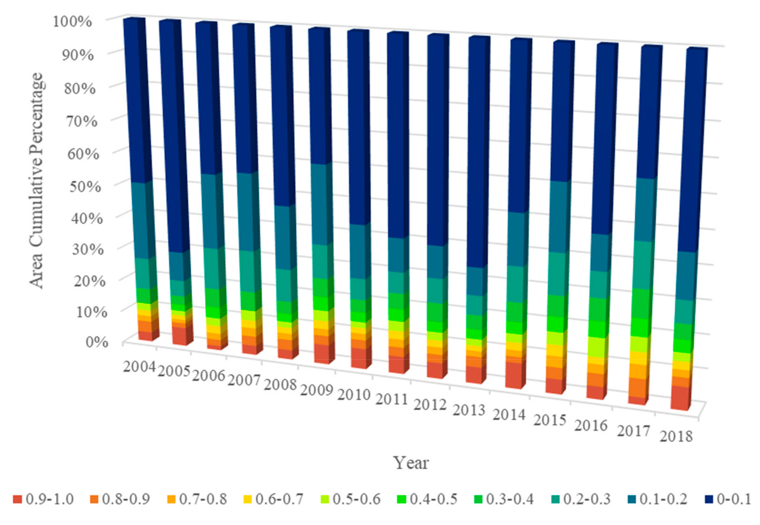
3.1.1. Daytime Spatiotemporal Variation in the FP
3.1.2. Nighttime Spatiotemporal Variation in FPs
3.2. Comparative Analysis of SUHI FPs Obtained by Gaussian Surface Model and Logistic Model
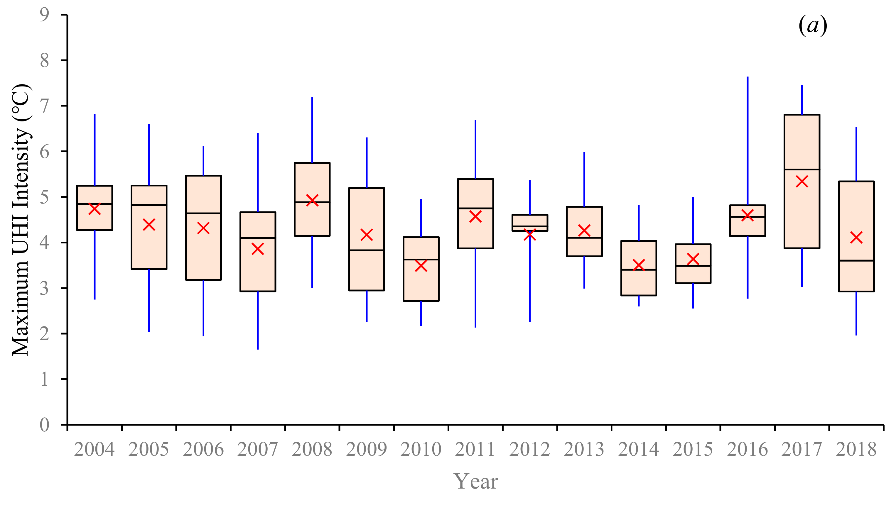
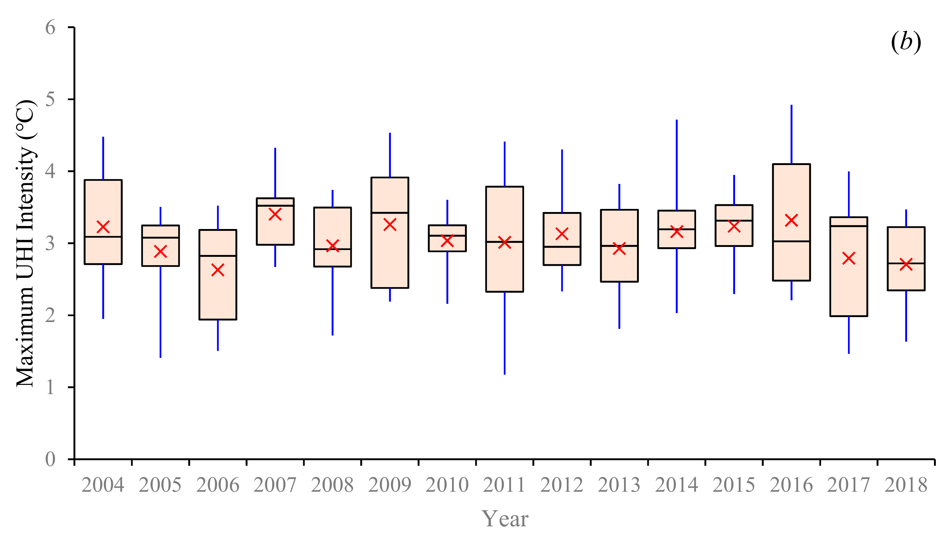
3.3. Temporal Changes in UHII
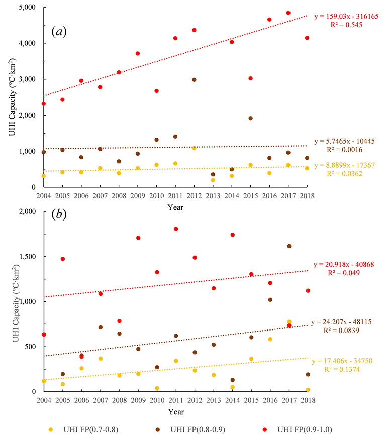
3.4. Temporal Changes in UHI Capacity
4. Discussion
4.1. Elimination of Artificial Bias in Background Temperatures
4.2. Enhanced Reliability of Remote Sensing Data and Surface Attribute
4.3. Relationship Between SUHI FP and UHII
5. Conclusions
Supplementary Materials
Author Contributions
Funding
Acknowledgments
Conflicts of Interest
References
- Oke, T.R. The energetic basis of the urban heat island. Q. J. R. Meteorol. Soc. 1982, 108, 1–24. [Google Scholar] [CrossRef]
- Yang, J.; Guo, A.D.; Li, Y.H.; Zhang, Y.Q.; Li, X.M. Simulation of landscape spatial layout evolution in rural-urban fringe areas: A case study of Ganjingzi District. GISci. Remote Sens. 2019, 56, 388–405. [Google Scholar] [CrossRef]
- Zhao, M.; Cai, H.; Qiao, Z.; Xu, X. Influence of urban expansion on the urban heat island effect in Shanghai. Int. J. Geogr. Inf. Sci. 2016, 30, 2421–2441. [Google Scholar] [CrossRef]
- Arnfield, A.J. Two decades of urban climate research: A review of turbulence, exchanges of energy and water, and the urban heat island. Int. J. Clim. 2003, 23, 1–26. [Google Scholar] [CrossRef]
- Oke, T.R. The urban energy balance. Prog. Phys. Geogr. Earth Env. 1988, 12, 471–508. [Google Scholar] [CrossRef]
- Rizwan, A.M.; Dennis, L.Y.C.; Liu, C. A review on the generation, determination and mitigation of urban heat island. J. Env. Sci. 2008, 20, 120–128. [Google Scholar] [CrossRef]
- Zhao, L.; Lee, X.; Smith, R.B.; Oleson, K. Strong contributions of local background climate to urban heat islands. Nature 2014, 511, 216–219. [Google Scholar] [CrossRef]
- Clinton, N.; Gong, P. Modis detected surface urban heat islands and sinks: Global locations and controls. Remote Sens. Env. 2013, 134, 294–304. [Google Scholar] [CrossRef]
- Li, X.; Zhou, Y.; Asrar, G.R.; Imhoff, M.; Li, X. The surface urban heat island response to urban expansion: A panel analysis for the conterminous United States. Sci. Total Env. 2017, 605, 426–435. [Google Scholar] [CrossRef]
- Liao, W.L.; Liu, X.P.; Wang, D.G.; Sheng, Y.L. The impact of energy consumption on the surface urban heat island in China’s 32 major cities. Remote Sens. 2017, 9, 250. [Google Scholar] [CrossRef]
- Peng, S.; Piao, S.; Ciais, P.; Friedlingstein, P.; Ottle, C.; Breon, F.-M.; Nan, H.; Zhou, L.; Myneni, R.B. Surface urban heat island across 419 global big cities. Env. Sci. Technol. 2012, 46, 696–703. [Google Scholar] [CrossRef] [PubMed]
- Zhou, D.; Zhao, S.; Liu, S.; Zhang, L.; Zhu, C. Surface urban heat island in China’s 32 major cities: Spatial patterns and drivers. Remote Sens. Env. 2014, 152, 51–61. [Google Scholar] [CrossRef]
- Oke, T.R.; Mills, G.; Voogt, J.A. Urban Climates; Cambridge University Press: Cambridge, UK, 2017. [Google Scholar]
- Cui, Y.; Xu, X.; Dong, J.; Qin, Y. Influence of urbanization factors on surface urban heat island intensity: A comparison of countries at different developmental phases. Sustainability 2016, 8, 706. [Google Scholar] [CrossRef]
- Imhoff, M.L.; Zhang, P.; Wolfe, R.E.; Bounoua, L. Remote sensing of the urban heat island effect across biomes in the continental USA. Remote Sens. Env. 2010, 114, 504–513. [Google Scholar] [CrossRef] [Green Version]
- Qiao, Z.; Tian, G.; Zhang, L.; Xu, X. Influences of urban expansion on urban heat island in Beijing during 1989–2010. Adv. Meteorol. 2014, 2014, 1–11. [Google Scholar] [CrossRef]
- Zhou, D.; Zhao, S.; Zhang, L.; Sun, G.; Liu, Y. The footprint of urban heat island effect in China. Sci. Rep. 2015, 5, 11160. [Google Scholar] [CrossRef]
- Chen, W.; Zhang, Y.; Peng, C.; Gao, W. Evaluation of urbanization dynamics and its impacts on surface heat islands: A case study of Beijing, China. Remote Sens. 2017, 9, 453. [Google Scholar] [CrossRef]
- Qiao, Z.; Xu, X.; Wu, F.; Luo, W.; Wang, F.; Liu, L.; Sun, Z. Urban ventilation network model: A case study of the core zone of capital function in Beijing metropolitan area. J. Clean. Prod. 2017, 168, 526–535. [Google Scholar] [CrossRef]
- Qiao, Z.; Wu, C.; Huang, N.; Xu, X.; Sun, Z.; Sun, X. Spatio-temporal structure of the urban thermal environment in Beijing based on an empirical orthogonal function. J. Spat. Sci. 2018, 63, 297–310. [Google Scholar] [CrossRef]
- Qiao, Z.; Zhang, D.; Xu, X.; Liu, L. Robustness of satellite-derived land surface parameters to urban land surface temperature. Int. J. Remote Sens. 2019, 40, 1858–1874. [Google Scholar] [CrossRef]
- Yang, J.; Su, J.R.; Xia, J.H.; Jin, C.; Li, X.M.; Ge, Q.S. The impact of spatial form of urban architecture on the urban thermal environment: A case study of the Zhongshan district, Dalian, China. IEEE J. Sel. Top. Appl. Earth Obs. Remote Sens. 2018, 11, 2709–2716. [Google Scholar] [CrossRef]
- Yang, J.; Jin, S.H.; Xiao, X.M.; Jin, C.; Xia, J.H.; Li, X.M.; Wang, S.J. Local climate zone ventilation and urban land surface temperatures: Towards a performance-based and wind-sensitive planning proposal in megacities. Sustain. Cities Soc. 2019, 47, 1–11. [Google Scholar] [CrossRef]
- Zhou, D.C.; Xiao, J.F.; Bonafoni, S.; Berger, C.; Deilami, K.; Zhou, Y.Y.; Frolking, S.; Yao, R.; Qiao, Z.; Sobrino, J.A. Satellite remote sensing of surface urban heat islands: Progress, challenges, and perspectives. Remote Sens. 2019, 11, 48. [Google Scholar] [CrossRef]
- Lai, J.; Zhan, W.; Huang, F.; Quan, J.; Hu, L.; Gao, L.; Ju, W. Does quality control matter? Surface urban heat island intensity variations estimated by satellite-derived land surface temperature products. ISPRS J. Photogramm. Remote Sens. 2018, 139, 212–227. [Google Scholar] [CrossRef]
- Li, H.; Zhou, Y.; Li, X.; Meng, L.; Wang, X.; Wu, S.; Sodoudi, S. A new method to quantify surface urban heat island intensity. Sci. Total Environ. 2018, 624, 262–272. [Google Scholar] [CrossRef] [PubMed]
- Gawuc, L.; Struzewska, J. Impact of MODIS quality control on temporally aggregated urban surface temperature and long-term surface urban heat island intensity. Remote Sens. 2016, 8, 374. [Google Scholar] [CrossRef]
- Memon, R.A.; Leung, D.Y.; Liu, C.H. An investigation of urban heat island intensity (UHII) as an indicator of urban heating. Atmos. Res. 2009, 94, 491–500. [Google Scholar] [CrossRef]
- Wang, J.; Huang, B.; Fu, D.; Atkinson, P.M. Spatiotemporal variation in surface urban heat island intensity and associated determinants across major Chinese Cities. Remote Sens. 2015, 7, 3670–3689. [Google Scholar] [CrossRef]
- Yao, R.; Wang, L.; Huang, X.; Niu, Y.; Chen, Y.; Niu, Z. The influence of different data and method on estimating the surface urban heat island intensity. Ecol. Indic. 2018, 89, 45–55. [Google Scholar] [CrossRef]
- Zhao, S.; Zhou, D.; Liu, S. Data concurrency is required for estimating urban heat island intensity. Env. Pollut. 2016, 208, 118–124. [Google Scholar] [CrossRef]
- Zhou, B.; Rybski, D.; Kropp, J.P. On the statistics of urban heat island intensity. Geophys. Res. Lett. 2013, 40, 5486–5491. [Google Scholar] [CrossRef]
- Chen, X.L.; Zhao, H.M.; Li, P.X.; Yin, Z.Y. Remote sensing image-based analysis of the relationship between urban heat island and land use/cover changes. Remote Sens. Env. 2006, 104, 133–146. [Google Scholar] [CrossRef]
- Li, W.; Cao, Q.; Lang, K.; Wu, J. Linking potential heat source and sink to urban heat island: Heterogeneous effects of landscape pattern on land surface temperature. Sci. Total Env. 2017, 586, 457–465. [Google Scholar] [CrossRef] [PubMed]
- Qiao, Z.; Tian, G.; Xiao, L. Diurnal and seasonal impacts of urbanization on the urban thermal environment: A case study of Beijing using MODIS data. ISPRS J. Photogramm. Remote Sens. 2013, 85, 93–101. [Google Scholar] [CrossRef]
- Bohnenstengel, S.I.; Evans, S.; Clark, P.A.; Belcher, S.E. Simulations of the London urban heat island. Q. J. R. Meteorol. Soc. 2011, 137, 1625–1640. [Google Scholar] [CrossRef]
- Renard, F.; Alonso, L.; Fitts, Y.; Hadjiosif, A.; Comby, J. Evaluation of the effect of urban redevelopment on surface urban heat islands. Remote Sens. 2019, 11, 299. [Google Scholar] [CrossRef]
- Sobrino, J.A.; Oltra-Carrió, R.; Sòria, G.; Jiménez-Muñoz, J.C.; Franch, B.; Hidalgo, V.; Mattar, C.; Julien, Y.; Cuenca, J.; Romaguera, M.; et al. Evaluation of the surface urban heat island effect in the city of Madrid by thermal remote sensing. Int. J. Remote Sens. 2013, 34, 3177–3192. [Google Scholar] [CrossRef]
- Chen, F.; Liu, J.; Ge, Q. Pulling vs. pushing: effect of climate factors on periodical fluctuation of Russian and South Korean tourist demand in Hainan Island, China. Chin. Geogr. Sci. 2017, 27, 648–659. [Google Scholar] [CrossRef]
- Martin, P.; Baudouin, Y.; Gachon, P. An alternative method to characterize the surface urban heat island. Int. J. Biometeorol. 2015, 59, 849–861. [Google Scholar] [CrossRef]
- Azevedo, J.A.; Chapman, L.; Muller, C.L. Quantifying the daytime and night-time urban heat island in Birmingham, UK: A comparison of satellite derived land surface temperature and high resolution air temperature observations. Remote Sens. 2016, 8, 153. [Google Scholar] [CrossRef]
- Wang, K.; Wang, J.; Wang, P.; Sparrow, M.; Yang, J.; Chen, H. Influences of urbanization on surface characteristics as derived from the Moderate-Resolution Imaging Spectroradiometer: A case study for the Beijing metropolitan area. J. Geophys. Res. Atmos. 2007, 112, D22S06. [Google Scholar] [CrossRef]
- Wang, K.; Jiang, S.; Wang, J.; Zhou, C.; Wang, X.; Lee, X. Comparing the diurnal and seasonal variabilities of atmospheric and surface urban heat islands based on the Beijing urban meteorological network. J. Geophys. Res. Atmos. 2017, 122, 2131–2154. [Google Scholar] [CrossRef]
- Jin, M.L.; Dickinson, R.E.; Zhang, D.L. The footprint of urban areas on global climate as characterized by MODIS. J. Clim. 2005, 18, 1551–1565. [Google Scholar] [CrossRef]
- Santamouris, M.; Paraponiaris, K.; Mihalakakou, G. Estimating the ecological footprint of the heat island effect over Athens, Greece. Clim. Change 2007, 80, 265–276. [Google Scholar] [CrossRef]
- Yang, Q.; Huang, X.; Tang, Q. The footprint of urban heat island effect in 302 Chinese cities: Temporal trends and associated factors. Sci. Total Env. 2019, 655, 652–662. [Google Scholar] [CrossRef] [PubMed]
- Zhang, X.; Friedl, M.A.; Schaaf, C.B.; Strahler, A.H.; Schneider, A. The footprint of urban climates on vegetation phenology. Geophys. Res. Lett. 2004, 31, L12209. [Google Scholar] [CrossRef]
- Keeratikasikorn, C.; Bonafoni, S. Satellite images and Gaussian parameterization for an extensive analysis of urban heat islands in Thailand. Remote Sens. 2018, 10, 665. [Google Scholar] [CrossRef]
- Quan, J.; Chen, Y.; Zhan, W.; Wang, J.; Voogt, J.; Wang, M. Multi-temporal trajectory of the urban heat island centroid in Beijing, China based on a gaussian volume model. Remote Sens. Environ. 2014, 149, 33–46. [Google Scholar] [CrossRef]
- Streutker, D.R. A remote sensing study of the urban heat island of Houston, Texas. Int. J. Remote Sens. 2002, 23, 2595–2608. [Google Scholar] [CrossRef]
- Yang, J.; Sun, J.; Ge, Q.S.; Li, X.M. Assessing the Impacts of Urbanization-Associated Green Space on Urban Land Surface Temperature: A Case Study of Dalian, China. Urban For. Urban Green. 2017, 22, 1–10. [Google Scholar] [CrossRef]
- Sun, R.; Chen, L. How can urban water bodies be designed for climate adaptation? Landsc. Urban Plan. 2012, 105, 27–33. [Google Scholar] [CrossRef]
- Sun, R.; Xie, W.; Chen, L. A landscape connectivity model to quantify contributions of heat sources and sinks in urban regions. Landsc. Urban Plan. 2018, 178, 43–50. [Google Scholar] [CrossRef]
- Xu, X.; Cai, H.; Qiao, Z.; Wang, L.; Jin, C.; Ge, Y.N.; Wang, L.Y.; Xu, F.J. Impacts of park landscape structure on thermal environment using QuickBird and Landsat images. Chin. Geogr. Sci. 2017, 27, 818–826. [Google Scholar] [CrossRef]
- Zhou, W.; Huang, G.; Cadenasso, M.L. Does spatial configuration matter? Understanding the effects of land cover pattern on land surface temperature in urban landscapes. Landsc. Urban Plan. 2011, 102, 54–63. [Google Scholar] [CrossRef]
- Zhou, W.; Qian, Y.; Li, X.; Li, W.; Han, L. Relationships between land cover and the surface urban heat island: Seasonal variability and effects of spatial and thematic resolution of land cover data on predicting land surface temperatures. Landsc. Ecol. 2014, 29, 153–167. [Google Scholar] [CrossRef]
- Meng, Q.; Zhang, L.; Sun, Z.; Meng, F.; Wang, L.; Sun, Y. Characterizing spatial and temporal trends of surface urban heat island effect in an urban main built-up area: A 12-year case study in Beijing, China. Remote Sens. Environ. 2018, 204, 826–837. [Google Scholar] [CrossRef]
- Liu, J.; Cheng, H.; Jiang, D.; Huang, L. Impact of climate-related changes to the timing of autumn foliage colouration on tourism in Japan. Tourism Manage. 2019, 70, 262–272. [Google Scholar] [CrossRef]
- Liu, J.Y.; Liu, M.L.; Tian, H.Q. Spatial and temporal patterns of China’s cropland during 1990–2000: An analysis based on Landsat TM data. Remote Sens. Env. 2005, 98, 442–456. [Google Scholar] [CrossRef]
- Gong, P.; Liu, H.; Zhang, M.; Li, C.; Wang, J.; Huang, H.; Clinton, N.; Ji, L.; Li, W.; Bai, Y.; et al. Stable classification with limited sample: Transferring a 30-m resolution sample set collected in 2015 to mapping 10-m resolution global land cover in 2017. Sci. Bull. 2019, 64, 370–373. [Google Scholar] [CrossRef]
- Feng, L.; Guo, S.; Zhu, L.J.; Zhou, Y.N.; Lu, D. Urban vegetation phenology analysis using high spatio-temporal NDVI time series. Urban For. Urban Green. 2017, 25, 43–57. [Google Scholar] [CrossRef]
- Villegas, D.; Aparicio, N.; Blanco, R.; Royo, C. Biomass accumulation and main stem elongation of durum wheat grown under Mediterranean conditions. Ann. Bot. 2001, 88, 617–627. [Google Scholar] [CrossRef]
- Zhang, X.; Friedl, M.A.; Schaaf, C.B.; Strahler, A.H.; Hodges, J.C.; Gao, F.; Reed, B.C.; Huete, A. Monitoring vegetation phenology using MODIS. Remote Sens. Env. 2003, 84, 471–475. [Google Scholar] [CrossRef]
- Zhang, Q.; Bilsborrow, R.E.; Song, C.; Tao, S.; Huang, Q. Determinants of out-migration in rural China: Effects of payments for ecosystem services. Popul. Environ. 2018, 40, 182–203. [Google Scholar] [CrossRef]
- Zhang, Q.; Bilsborrow, R.E.; Song, C.; Tao, S.; Huang, Q. Rural household income distribution and inequality in China: Effects of payments for ecosystem services policies and other factors. Ecol. Econ. 2019, 160, 114–127. [Google Scholar] [CrossRef]
- Liu, C.; Zhang, Q.; Luo, H.; Qi, S.; Tao, S.; Xu, H.; Yao, Y. An efficient approach to capture continuous impervious surface dynamics using spatial-temporal rules and dense Landsat time series stacks. Remote Sens. Env. 2019, 229, 114–132. [Google Scholar] [CrossRef]
- Zhang, Q.; Song, C.; Chen, X. Effects of China’s payment for ecosystem services programs on cropland abandonment: A case study in Tiantangzhai Township, Anhui, China. Land Use Policy 2018, 73, 239–248. [Google Scholar] [CrossRef]
- Wang, Y.; Li, X.; Zhang, Q.; Li, J.; Zhou, X. Projections of future land use changes: Multiple scenarios-based impacts analysis on ecosystem services for Wuhan city, China. Ecol. Indic. 2018, 94, 430–445. [Google Scholar] [CrossRef]
- Liu, J.; Wang, J.; Wang, S.; Wang, J.; Deng, G. Analysis and simulation of the spatiotemporal evolution pattern of tourism lands at the Natural World Heritage Site Jiuzhaigou, China. Habitat Int. 2018, 79, 74–88. [Google Scholar] [CrossRef]


| The Probability Levels of SUHI FPs | Gaussian Surface Model | Logistic Model | ||
|---|---|---|---|---|
| Daytime | Nighttime | Daytime | Nighttime | |
| 0.0–0.1 | 9823 | 6723 | 8128 | 5180 |
| 0.1–0.2 | 712 | 1678 | 934 | 2557 |
| 0.2–0.3 | 567 | 1083 | 672 | 1983 |
| 0.3–0.4 | 329 | 1014 | 614 | 1237 |
| 0.4–0.5 | 436 | 683 | 523 | 772 |
| 0.5–0.6 | 259 | 357 | 525 | 658 |
| 0.6–0.7 | 202 | 307 | 508 | 529 |
| 0.7–0.8 | 156 | 172 | 563 | 610 |
| 0.8–0.9 | 166 | 256 | 612 | 808 |
| 0.9–1.0 | 2004 | 2381 | 1575 | 320 |
© 2019 by the authors. Licensee MDPI, Basel, Switzerland. This article is an open access article distributed under the terms and conditions of the Creative Commons Attribution (CC BY) license (http://creativecommons.org/licenses/by/4.0/).
Share and Cite
Qiao, Z.; Wu, C.; Zhao, D.; Xu, X.; Yang, J.; Feng, L.; Sun, Z.; Liu, L. Determining the Boundary and Probability of Surface Urban Heat Island Footprint Based on a Logistic Model. Remote Sens. 2019, 11, 1368. https://0-doi-org.brum.beds.ac.uk/10.3390/rs11111368
Qiao Z, Wu C, Zhao D, Xu X, Yang J, Feng L, Sun Z, Liu L. Determining the Boundary and Probability of Surface Urban Heat Island Footprint Based on a Logistic Model. Remote Sensing. 2019; 11(11):1368. https://0-doi-org.brum.beds.ac.uk/10.3390/rs11111368
Chicago/Turabian StyleQiao, Zhi, Chen Wu, Dongqi Zhao, Xinliang Xu, Jilin Yang, Li Feng, Zongyao Sun, and Luo Liu. 2019. "Determining the Boundary and Probability of Surface Urban Heat Island Footprint Based on a Logistic Model" Remote Sensing 11, no. 11: 1368. https://0-doi-org.brum.beds.ac.uk/10.3390/rs11111368