Geographically Weighted Machine Learning and Downscaling for High-Resolution Spatiotemporal Estimations of Wind Speed

1
State Key Laboratory of Resources and Environmental Information Systems, Institute of Geographic Sciences and Natural Resources Research, Chinese Academy of Sciences, Datun Road, Beijing 100101, China
2
University of Chinese Academy of Sciences, Beijing 100049, China
Remote Sens. 2019, 11(11), 1378; https://0-doi-org.brum.beds.ac.uk/10.3390/rs11111378
Submission received: 27 March 2019
/
Revised: 1 June 2019
/
Accepted: 7 June 2019
/
Published: 10 June 2019
(This article belongs to the Section Atmospheric Remote Sensing)
Abstract
:High-resolution spatiotemporal wind speed mapping is useful for atmospheric environmental monitoring, air quality evaluation and wind power siting. Although modern reanalysis techniques can obtain reliable interpolated surfaces of meteorology at a high temporal resolution, their spatial resolutions are coarse. Local variability of wind speed is difficult to capture due to its volatility. Here, a two-stage approach was developed for robust spatiotemporal estimations of wind speed at a high resolution. The proposed approach consists of geographically weighted ensemble machine learning (Stage 1) and downscaling based on meteorological reanalysis data (Stage 2). The geographically weighted machine learning method is based on three base learners, which are an autoencoder-based deep residual network, XGBoost and random forest, and it incorporates spatial autocorrelation and heterogeneity to boost the ensemble predictions. With reanalysis data, downscaling was introduced in Stage 2 to reduce bias and spatial abrupt (non-natural) variation in the predictions inferred from Stage 1. The autoencoder-based residual network was used in Stage 2 to adjust the difference between the averages of the fine-resolution predicted values and the coarse-resolution reanalysis data to ensure consistency. Using mainland China as a case study, the geographically weighted regression (GWR) ensemble predictions were shown to perform better than individual learners’ predictions (with an approximately 12–16% improvement in R2 and a decrease of 0.14–0.19 m/s in root mean square error). Downscaling further improved the predictions by reducing inconsistency and obtaining better spatial variation (smoothing). The proposed approach can also be applied for the high-resolution spatiotemporal estimation of other meteorological parameters or surface variables involving remote sensing images (i.e. reliable coarsely resolved data), ground monitoring data and other relevant factors.

1. Introduction
High-resolution spatiotemporal mapping of surface variables can present specific variation at fine spatial and temporal scales, which provides good knowledge of the spatiotemporal distribution of these variables. For wind speed, this technique is particularly useful for atmospheric environmental monitoring [1,2,3], air quality evaluation [4,5,6,7], wind power siting [8], and so on. Recently, meteorological reanalysis [9,10,11] has been employed in numeric weather prediction models with historic weather observations from multiple sources, including satellites and surface stations, to generate images with more reliable estimates at high temporal resolutions, which are a relatively new source of meteorological data. At a high temporal resolution (e.g., 3 h), the reanalysis data are still at a coarse spatial resolution [e.g., 0.25° (latitude) × 0.3125° (longitude)], and thus cannot provide local variations at a fine spatial scale for wind speed, which is affected by prevailing pressure, air temperature and local site characteristics with a volatile nature. Additionally, such finely resolved variability of wind speed also might not be captured well (low accuracy) by traditional approaches, including multiple linear regression [12], nonlinear regression [13] and spatial interpolation [14,15] (e.g., inverse distance weighting or kriging) due to the sparse spatial distribution of wind speed monitoring stations, and the limited generalization of these methods compared to advanced machine learning methods, such as XGBoost and deep learning.
Currently, in addition to classic climate models [16], advanced machine learning techniques, such as support vector machines [17], neural networks [18,19], hybrid and ensemble machine learning [20], and deep learning [21] are increasingly employed for time series forecasting of meteorological factors. For wind speed with high volatility and randomness, machine learning can achieve good performance, as demonstrated in many applications [8]. However, most of these approaches are based on individual learners or ensemble learning methods based on limited or weak individual learners, and the output’s spatial resolution is very limited. For high-resolution spatiotemporal wind speed mapping, few studies have reported the use of advanced machine learning with reliable performance. Individual learners, which were mostly used in previous approaches, may deeply learn the irregularities in the training samples due to the influence of sampling bias, which often leads to overfitting for new datasets. Ensemble machine learning provides a solution that can mitigate this potential issue, given that the ensemble averages of multiple models with acceptable accuracy can effectively reduce bias and variance [22,23]. However, ensemble learning by averaging does not consider geospatial heterogeneity that, if significant, may bias the final predictions.
Reanalysis data are widely used in a variety of domains, including weather and climate forecasting, due to their reliability, which is based on their hybrid origins. Practitioners frequently refer to reanalysis data as benchmark “observations” [24]. Due to their coarse resolution, they are seldom directly used in high-resolution meteorological mapping. With downscaling [25], reanalysis data can be used as the original coarse-resolution background information for finely resolved mapping. For the downscaling of continua, area-to-point prediction (ATPP) techniques, such as area-to-point kriging [26], Poisson kriging [27], and cokriging [28], are widely used as interpolations. However, kriging-based ATPP methods need to reliably fit variogram, which may not be suitable for the simulation of volatile wind speeds. Given practical applications, an autoencoder-based deep residual network can be employed to capture the quantitative relationship between coarse- and fine-resolution wind speeds. With a large and flexible network architecture, an autoencoder-based deep residual network has robust generalization in practical applications [29]. Downscaling with reanalysis data can reduce the bias and obtain better spatial variation (smoothing) in predictions and improve integrity.
In this study, for high-resolution spatiotemporal wind speed mapping, a two-stage approach of geographically weighted ensemble machine learning and downscaling with reanalysis data was developed. The former is based on three base learners: an autoencoder-based residual net, XGBoost and random forest. The learners were selected due to the considerable differences in their model structures and their good performance in practical applications. Compared with traditional learners, such as the nonlinear generalized additive model (GAM) and feed-forward neural networks, the three learners may have higher learning efficiency and better performance. Although the support vector machine can obtain a globally optimal solution, its scalability is constrained by a big sample size, and choosing appropriate hyperparameters and kernel functions is time-consuming and requires expert knowledge. The fuzzy neural system is based on fuzzy and artificial neural networks, and its main drawback is slow convergence for regression [30,31]. As a spatial modeling method, kriging involves variogram simulation which is considerably limited by the sparse distribution of monitoring stations and wind speed volatility. Comparatively, the three base learners used in Stage 1 are easy to train, achieve acceptable performance and require fewer manual feature engineering operations.
Theoretically, models that have no correlations or weak correlations can better improve their ensemble predictions, and strong learners can prevent ensemble predictions below their individual performance levels. To ensure high-resolution spatiotemporal mapping of meteorological factors with reasonable spatial variation at a fine local scale, the proposed approach used relevant covariates, including coordinates, time indices, elevations and reanalysis data (e.g., wind speed and planetary boundary layer height (PBLH)) from multiple sources. Coarse spatial resolution meteorological reanalysis data were used as a priori knowledge to capture spatiotemporal variations in the target variables at a regional scale [10] and were used in both individual learners and downscaling in the proposed approach. Resampling was also used to adjust and align the images at different origins and spatial resolutions.
In the proposed approach, geographically weighted regression (GWR) was conducted over the three learners’ predictions to detect the spatial variability of their performances. GWR can take full advantage of the abilities of the three modern regression models by considering spatial heterogeneity for robust prediction. A case study of mainland China was conducted for wind speeds that are hard to map at a high resolution due to their implicit volatility. In the wind speed case study, the approach proposed in this paper was demonstrated to be applicable for the high-resolution spatiotemporal mapping of meteorological parameters and other surface variables that involve remote sensing (including reliable coarse-resolution data), ground monitoring data and other factors.
2. Study Region and Materials
2.1. Study Region
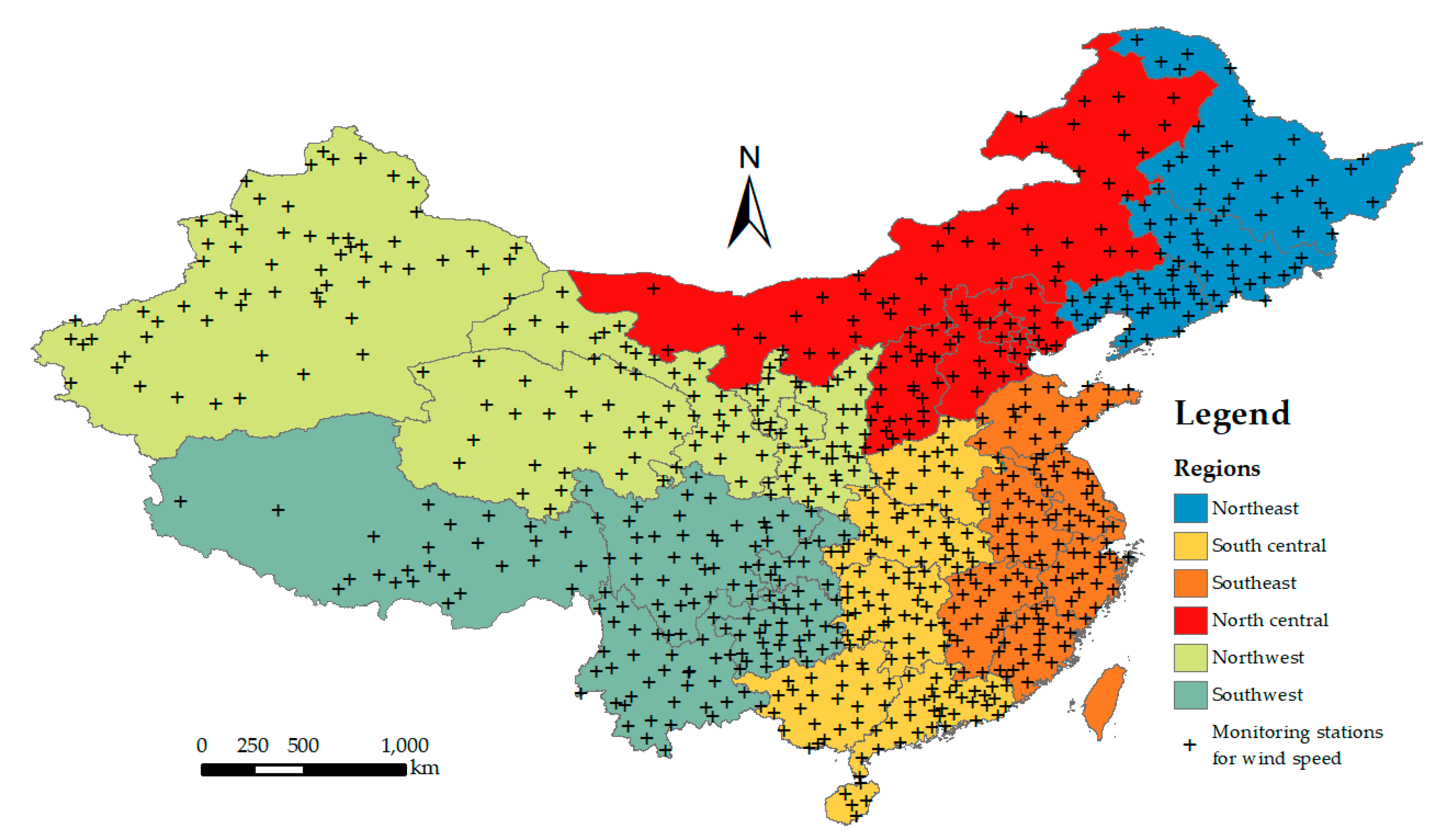
The study region (Figure 1) is mainland China with geographical coverage of 73°27′ to 135°06′ east longitude and 18°11′ to 53°33′ north latitude and an area of 9,457,770 square kilometers. In mainland China, the climate varies from region to region due to its massive geographical coverage and diversity of landforms and elevations. In the northeast, it is hot and dry in the summer and freezing cold in the winter. In the southwest, there is plenty of rainfall in the semitropical summers and cool winters. The major influential factors include the geographic latitude, solar radiation, distribution of land and sea, ocean currents, topology and atmospheric circulation. Thus, it is challenging to map the high-resolution spatiotemporal surfaces of meteorological factors such as wind speed for such a large region with considerable heterogeneity between regions.
2.2. Measurement Data
The ground monitoring station measurement data originated from the daily ground observation datasets of individual years for mainland China from the China Meteorological Data Service Center (http://data.cma.cn). The dataset was collected based on 824 national base meteorological monitoring stations. The 2015 daily wind speed data (unit: meter/second, abbreviated as m/s) measured at a height of 10–12 m above the ground were collected. Quality assurance was conducted to remove noisy samples. The final number of monitoring stations was 770. The target variable to be predicted was wind speed. The output mapping surfaces were at a spatial resolution of 1 km (projected coordinate system: Beijing 1954 with Krassowsky 1940, European Petroleum Survey Group (EPSG): 4214; https://epsg.io/4214) and a temporal resolution of 1 day. Figure 1 also shows the spatial distribution of the wind speed monitoring stations.
2.3. Covariates
According to influential factors and data accessibility, the following covariates were selected.
(1) Coordinates
Latitude and longitude were used to capture differences in locations and the related geographical environment for meteorological factors. The quadratic transformations of the coordinates and their products (to reflect the interaction of latitude and longitude) were derived to reflect the diversity and complexity of the landforms. While many machine learning algorithms, such as neural networks, XGBoost and random forest, cannot directly model spatial autocorrelation, the coordinates are used as proxies in these algorithms to partially account for spatial autocorrelation.
(2) Elevation
The diversity of elevation is also partially responsible for the considerable differences in the meteorology in mainland China. This study used elevation data with a 500m spatial resolution from the Shuttle Radar Topology Mission (SRTM; https://www2.jpl.nasa.gov/srtm/). SRTM was published in 2003 and covers more than 80% of the Earth’s land surface.
(3) Reanalysis data
As mentioned, meteorological reanalysis data were used to provide reliable coarse spatial resolution estimates. The reanalysis data were from the newest Goddard Earth Observing System-Forward Processing (GEOS-FP) dataset, which is based on the data assimilation system (DAS). GEOS-FP covers all of mainland China at a spatial resolution of 0.25° (latitude) × 0.3125° (longitude) and a temporal resolution of 3 h (ftp://rain.ucis.dal.ca/ctm/GEOS_0.25x0.3125_CH.d/GEOS_FP). The corresponding coarse-resolution data of wind speed was used. Furthermore, the PBLH was also extracted, since it is an important factor for the surface wind gradient and is closely related to wind speed [32,33].
Since the reanalysis data were at a coarse resolution, projection transformation and resampling were conducted to align the data in terms of origin and resolution for use as the inputs to individual learners.
(4) Day of the year
The day of the year was used to capture the temporal variation in the wind speed to be estimated.
(5) Regional separation
Given the diverse differential geographical, atmospheric and land-use settings across mainland China, a map (Figure 1) of the six regions of mainland China (northeast, north central, northwest, southwest, south center, and southeast) from the Resources and Environmental Data Cloud Platform (http://www.resdc.cn/) was employed to identify the regional qualitative factors in the models and account for the spatial heterogeneity of mainland China at the regional level.
3. Methods
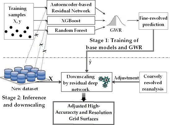
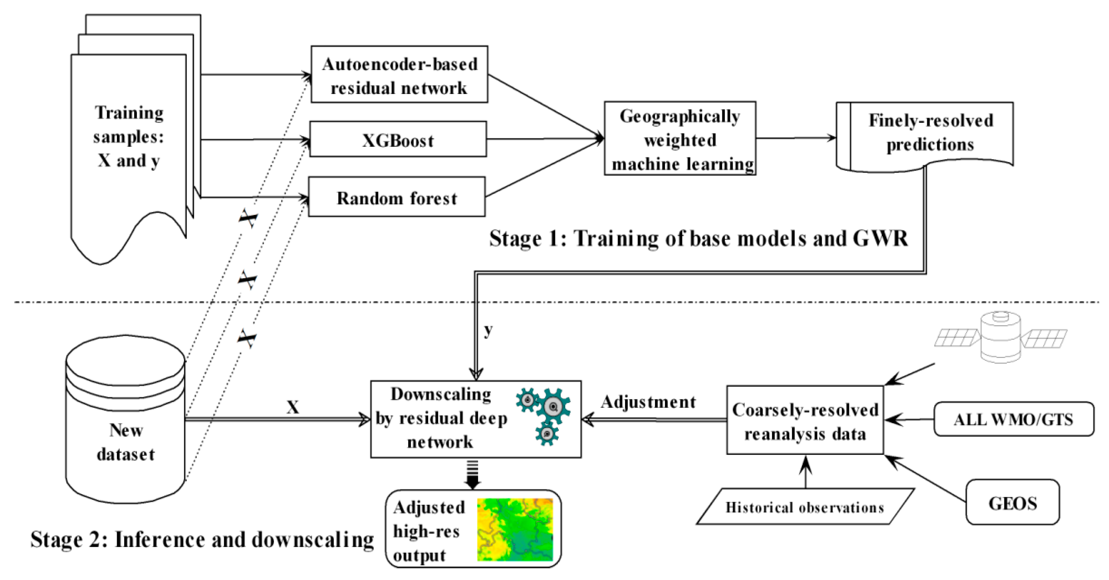
The systematic framework was based on two stages (Figure 2): (1) training and (2) inference and downscaling. In Stage 1, for the initial high-resolution prediction, three machine learning models, which were an autoencoder-based deep residual network, XGBoost and random forest, were trained, and GWR was used to fuse the outcomes from the three learners for ensemble predictions (Figure 3). In Stage 2, for high-resolution mapping of the new dataset, a deep residual network was iteratively used in downscaling to match the wind speed at a coarse resolution and the average wind speed at a fine resolution, which were initially inferred from Stage 1 to reduce the bias and obtain better spatial variation (smoothing) of the predictions.
3.1. Stage 1: Geographically Weighted Learning
Stage 1 aims to train three representative base models to improve the ensemble estimates using GWR, which presents reliable fine-resolution spatiotemporal contrasts or variability.
3.1.1. Base Learners
In ensemble learning, models with no correlations or weak correlations can theoretically generate better ensemble predictions with less error [23]. Assume m models with errors εi (i = 1, …, m, denoting the model indices) drawn from a zero-mean multivariate normal distribution with variances and covariances . Then, the error made by their average prediction is . The expected squared error of the ensemble prediction is:
where c represents the covariance between the errors of different models. If c is equal to 0, which indicates no correlation between the errors of the models, then the expected squared error of the ensemble averages is of the error variances, ν. However, if c is equal to ν, indicating a perfect correlation between the models’ errors, the expected squared error is equal to the error variances, ν, suggesting no change for the ensemble prediction errors. Therefore, the selection of models that have no correlations or weak correlations is crucial for improving ensemble predictions.
Furthermore, if a base model is robust, indicating small errors, the expected squared error of the ensemble predictions can be reduced to a value that may be lower than ν according to (1). Thus, three typical models (an autoencoder-based deep residual network [29], XGBoost [34] and random forest [35]) were selected. The deep residual network has a completely different structure from the other two models (XGBoost and random forests), which are based on a decision tree. However, the optimization approaches of XGBoost and random forest are different, with the former using gradient boost and the latter using bootstrap aggregating (bagging). Thus, the three models are quite different and robust in practical applications [29,34,36,37]. Other learners, such as AdaBoost or Gaussian process regression, can also be considered. To simplify application and illustrate a geographically weighted machine learning method, these three typical learners were used as the robust base learners in the geographically weighted modeling, as their ensemble predictions have sufficiently competitive performance for this paper’s case study.
(1) Autoencoder-based deep residual network
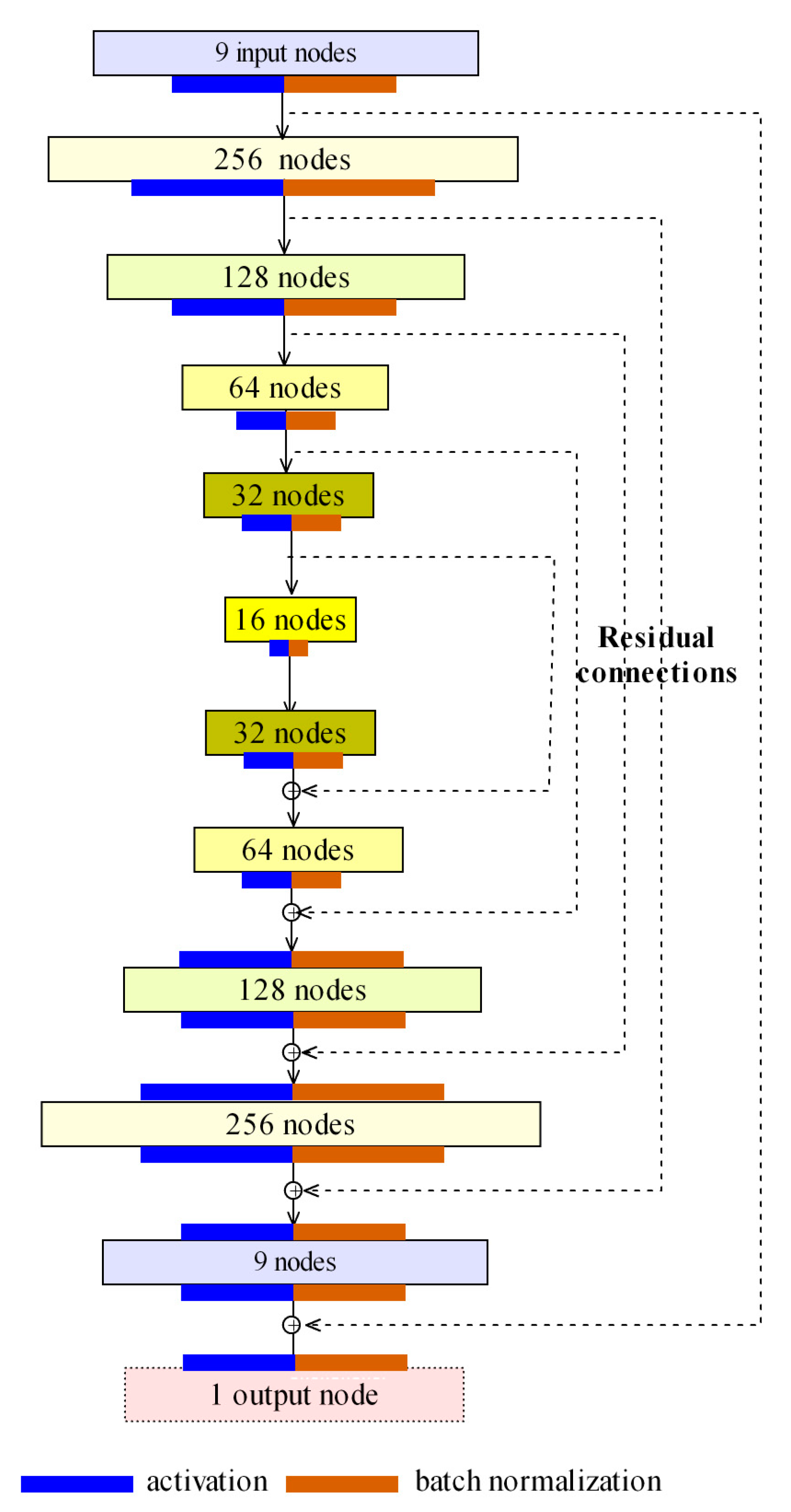
In this approach, the autoencoder provides the basic infrastructure for the network so that residual mapping can be implemented by an identity connection from the shallow layers in the encoding component to the deep layers in the decoding component [29]. Residual (shortcut) connections in neural networks have been demonstrated to address vanishing/exploding gradients [38] and accuracy degradation in CNNs [39,40]. Based on similar ideas, residual connections were added into the autoencoder-based deep network to improve learning accuracy and efficiency, as demonstrated in practical applications [29]. The Keras-based packages of this approach for Python (https://pypi.org/project/resautonet) and R (https://cran.r-project.org/web/packages/resautonet) have been published, and examples can be retrieved online (https://github.com/lspatial/resautonet).
Figure 4 shows the network topology for the prediction of wind speed. This network has 9 input nodes to represent 9 covariates (latitude, longitude, squares of latitude and longitude, products of latitude and longitude, elevation, GEOS-FP wind speed, GEOS-FP PBLH, and the day of the year). For the internal autoencoder, the network structure of the encoding component consists of 4 hidden layers (the number of nodes for each layer in sequence: [256, 128, 64, 32]), the middle coding layer has 16 nodes; correspondingly, the decoding component consists of 4 hidden layers and the number of nodes of each layer is the inverse of that of the encoding component. The residual connection is added from shallow to deep layers. The final output is the target variable (high-resolution wind speed, m/s) to be predicted. The following loss function was used for optimization:
where y is the target variable (wind speed), x denotes the input covariates, is the mapping function with parameters of W and b, and represents the elastic net regularizer [41] that linearly combines the L1 and L2 penalties. Throughout this paper, the autoencoder-based deep residual network was also referred to as a (deep) residual network.
(2) XGBoost
XGBoost is a scalable end-to-end tree boosting learning system that is widely used to achieve state-of-the-art results in many domains [34]. XGBoost uses a sparsity-aware algorithm and a cache-aware block structure for efficient tree learning.
Assume n examples and d features, . Additive functions are used to make the final predictions [34]:
where K is the number of functions corresponding to each tree (K trees in total), f(x) = wq(x) represents the space of the regression trees (CART), and q represents the structure of each tree that maps an instance to a leaf.
Based on gradient tree boosting, XGBoost was trained in an additive manner. Assume the regularized loss function of step k is
where l is a differentiable differential loss function and Ω is the regularizer. To derive the optimal addition, fk(xi), the second-order approximation of the Taylor series can be employed to optimize the objective more efficiently than the first-order approximation:
where and are the first- and second-order gradient derivatives of the loss function in terms of the last prediction ().
Then, the optimal weights w can be obtained for a fixed tree structure, q. A greedy heuristic algorithm or approximate algorithms can be used to construct optimal trees according to the split score, that is, the loss reduction after the split, based on the optimal weights and loss. For details, please refer to [34]. There is an open-source library of XGBoost to support the R and Python interfaces (https://xgboost.readthedocs.io).
(3) Random forest
Random forest [42] is an improved version of bootstrap aggregating (bagging) with a decision tree as its base model. Bagging starts with sampling (with replacement) n (the sample size) training samples from the original samples; then, the trees are trained with a bootstrapped subsample. The final predictions are made by averaging the predictions from the individual regression trees, as follows:
where K is the number of trees, x represents the d-dimensional input and fk(x) is the output of the kth tree for x.
This bootstrapping procedure can achieve good performance because it can decrease the variance of the model without increasing the bias, which means that, while the predictions of a single tree are highly sensitive to noise in the training set, the average of many trees is not as long as the trees are not correlated. In random forest, in addition to the data examples, sampling with replacement is also implemented for the set of input features to decrease the correlation between the models. The Python’s scikit-learn machine learning library provides support for random forest (https://scikit-learn.org/stable/modules/ensemble.html).
3.1.2. Geographically Weighted Learning
For the three robust base models (the autoencoder-based deep residual network, XGBoost and random forest) and their averages, spatial autocorrelation cannot be directly embedded within the models and their predictions. Thus, GWR was proposed to obtain the optimal configuration (weights) of the three robust models and their spatial variations considering spatial autocorrelation and heterogeneity for a robust fused prediction (Figure 3).
GWR is a local regression method with a moving window or spatial kernel to constrain the domain of the samples for regression [43]. In GWR, spatial dependence is considered according to Tobler’s first law of geography (i.e., “everything is related to everything else, but near things are more related than distant things”) [44]. Assume that there is a sample of features, x (three features for this paper’s case study: the predictions of the three base learners) within the local domain, D, and that GWR considers location-specific regression coefficients:
where (ui,vi) are the coordinates of the ith sample, βk(ui,vi) is the regression coefficient for the kth base prediction, and εi is random noise (εi~N(0,1)).
With the weighted least square method, the following solution can be obtained:
where X is the input matrix of all examples, W is the spatial weight matrix of examples of the target location, (ui,vi), and y is the output vector. GWR is provided in the R spgwr package (https://cran.r-project.org/web/packages/spgwr/index.html).
For this study, the Gaussian kernel was used to quantify the spatial weight matrix, W:
where b is the bandwidth indicating the sampling domain and dij is the distance between locations i and j.
GWR can output the predictions and their variance by fusing the predictions from the three learners (the autoencoder-based deep residual network, XGBoost and random forest). Furthermore, by using spatially varying coefficients for each learner in GWR, each learner’s contribution to the integrated prediction and its spatial heterogeneity can also be presented.
For each of the three individual learners, all sample data from 2015 were used to train an integral model. Considering the implicit character of local regression for GWR and the considerable difference between different days for wind speed, daily GWR was conducted over daily predictions of individual learners to obtain the corresponding predictions.
3.2. Stage 2: Downscaling with A Deep Residual Network
For new datasets, Stage 2 aims to use reanalysis data or other reliable data at coarse resolution to adjust the output initially inferred from Stage 1, making the averages of the output at fine resolution and the value at the corresponding coarse resolution consistent (Figure 2). Reliable coarse-resolution data were used as a priori knowledge so that the ensemble predictions from Stage 1 were reasonable and conformed with the presumed trend at the background (coarse-resolution) scale. Downscaling began with the ensemble predictions from Stage 1 that captured spatiotemporal contrast or variability well at a finely local scale. Then, a deep residual network was iteratively used in downscaling to match the output at fine resolution and the values at coarse resolution until the threshold for their difference was attained. Except for the coarse-resolution target variable, the set of all other covariates of the new dataset were used to make predictions at fine resolution in downscaling. Assume the target variable value at a coarse-resolution grid cell, Gi, i = 1, …, C (C is the number of coarsely resolved grid cells), and at a fine-resolution grid cell, gi, i = 1, …, F (F is the number of finely resolved grid cells). Due to its good ability to capture nonlinear associations between the covariates and the target variable [29] and spatial continuity, an autoencoder-based deep residual network was used to model the relationship between the aforementioned covariates and gi at fine resolution with the following regularizer:
where Fl represents the set of finely resolved grid cells that overlay the lth coarsely resolved grid cell. This regularizer in equation (10) indicates that the average of the finely resolved grid cells within each coarsely resolved grid cell is equal to the grid value of the latter. Given the reliability of the coarsely resolved dataset (reanalysis data), this regularizer is reasonable as the constraint.
For implementation, the predicted values were adjusted for each finely resolved cell using the following formula to ensure equality in (10) and a deep residual network was used to update the regression in each iteration:
where Gl is assumed to be overlaid with gi, t represents the iteration time, and denotes the adjusted values for iteration t.
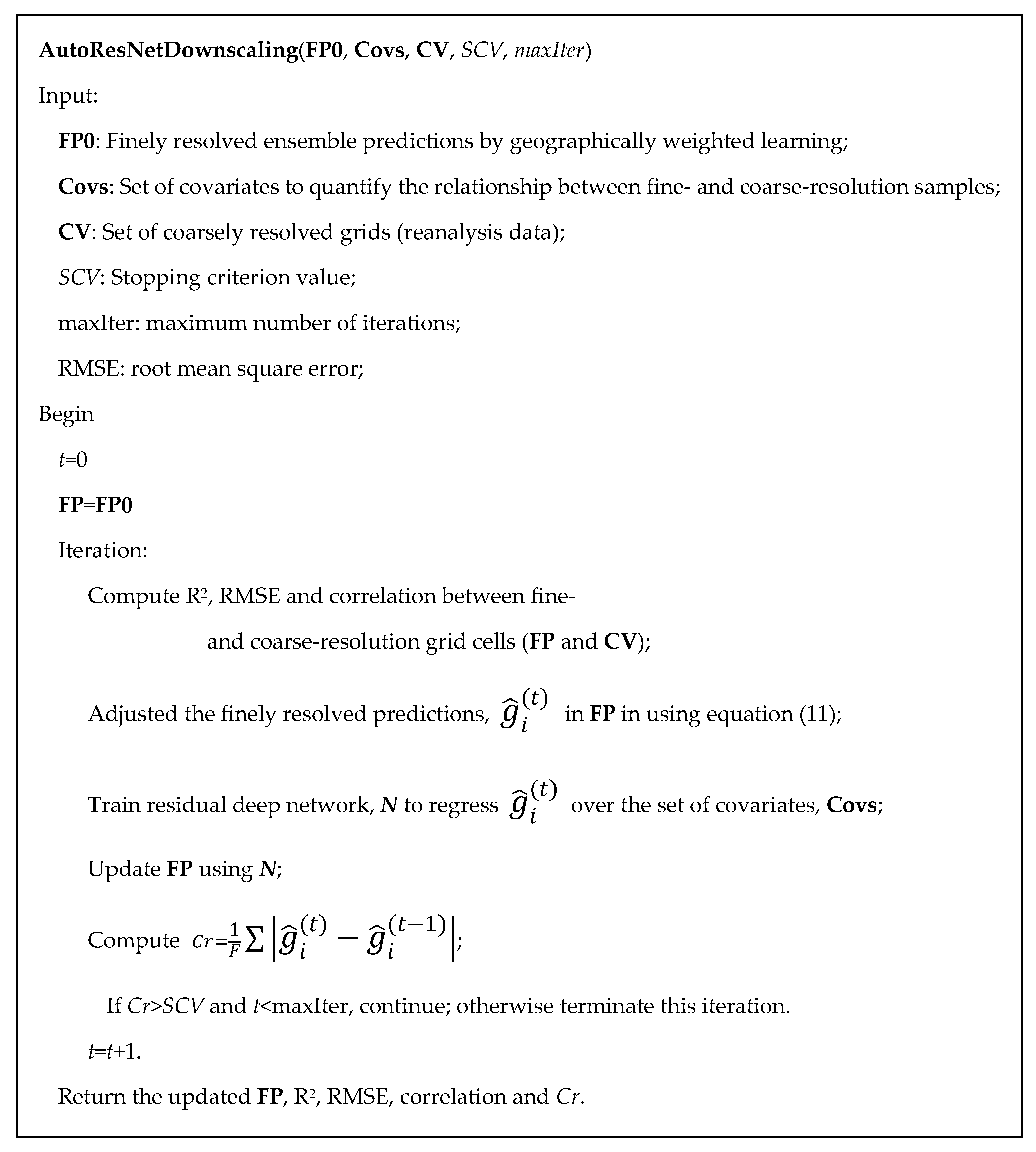
Iteration proceeded until the average over the absolute difference in the finely resolved grid cells between two continuous iterations, that is, , was equal to or below a stopping criterion value or the maximum number of iterations was attained. The complete algorithm is given in Figure 5. Additionally, an R package of this downscaling algorithm was published (https://github.com/lspatial/autoresnetR).
3.3. Optimization of Hyperparameters and Validation
To obtain robust wind speed predictions, empirical knowledge and a machine learning grid search were used to find the optimal hyperparameter values. For the autoencoder-based residual network, initial networks were constructed according to previous empirical knowledge and then refined using sensitivity analysis. A cross validation grid search for mini-batch size, network depth, output type and activation functions were conducted to find optimal solutions of these hyperparameters. For XGBoost, the grid consisted of maximum booting iterations (100, 200, 300, 400), maximum tree depths (6 to 12), learning rates (0.05, 0.5, 1), and so on, for an optimal search. For GWR, the grid consisted of different bandwidths (100 km, 200 km, 300 km, 400 km, 500 km) for the search.
For an independent test of Stage 1, 30% of the complete samples were sampled (stratified by region (Figure 1) and month) to validate each of the three individual models. This stratification sampling ensured even distribution of the samples across space and time to mitigate the overestimation of spatial results. Given the need for more samples for local regression, leave-one-site-out cross-validation (LOOCV) was conducted to validate GWR. Training (for all the models), independent test, and LOOCV (for GWR) coefficient of determination (R-squared, i.e. R2), adjusted R2, root mean square error (RMSE), and mean absolute error (MAE) were reported and compared in the results. For Stage 2, similar metrics (independent test R2 and RMSE) were reported for the autoencoder-based deep residual network to map the covariates to the finely resolved grids and for the coarse-resolution grid cells and the averages of the fine-resolution grid cells overlaid in downscaling.
For comparison with nonlinear GAM and the feed-forward neural network, the same samples used to train the base models in Stage 1 were used for training. Training and test R2, RMSE and MAE were also reported for both. To ensure fairness in comparison, except for residual connections, this feed-forward neural network had the same hidden layers and the same number (100, 959) of parameters as deep residual network. To diagnose potential spatial correlation in the residuals of ensemble predictions by GWR, Moran’s I was calculated for each day’s residuals [45]; variogram was also fitted for each day’s residuals, and consequently was used in universal kriging to estimate the corresponding day’s residuals. LOOCV R2 and RMSE were evaluated for original and estimated residuals of each day.
4. Results
4.1. Data Summary and Preprocessing
In total, 255,209 measurement samples with their covariates were collected from 770 wind speed monitoring stations across mainland China (see Figure 1 for the study region and spatial distribution of these monitoring stations). For 2015, the average daily wind speed was 2.1 m/s. Table 1 shows the statistics for the measurement samples and their partial covariates. A priori knowledge and the outer fences technique [46] were also used to filter out several invalid measurement samples.
The result (Supplementary Materials Figure S1) showed less skewness for log-transformed wind speed measurements than original measurements (2.45 vs. −0.56). Thus, for GWR, the wind speed measurements were log-transformed in the training samples.
4.2. Training of the Models in Stage 1
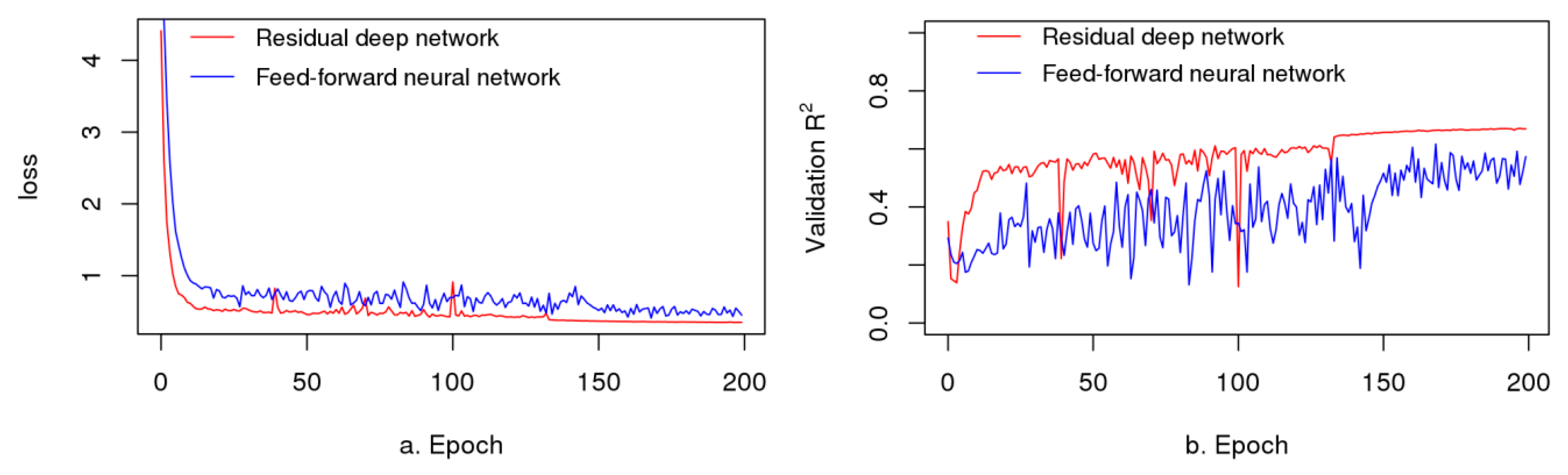
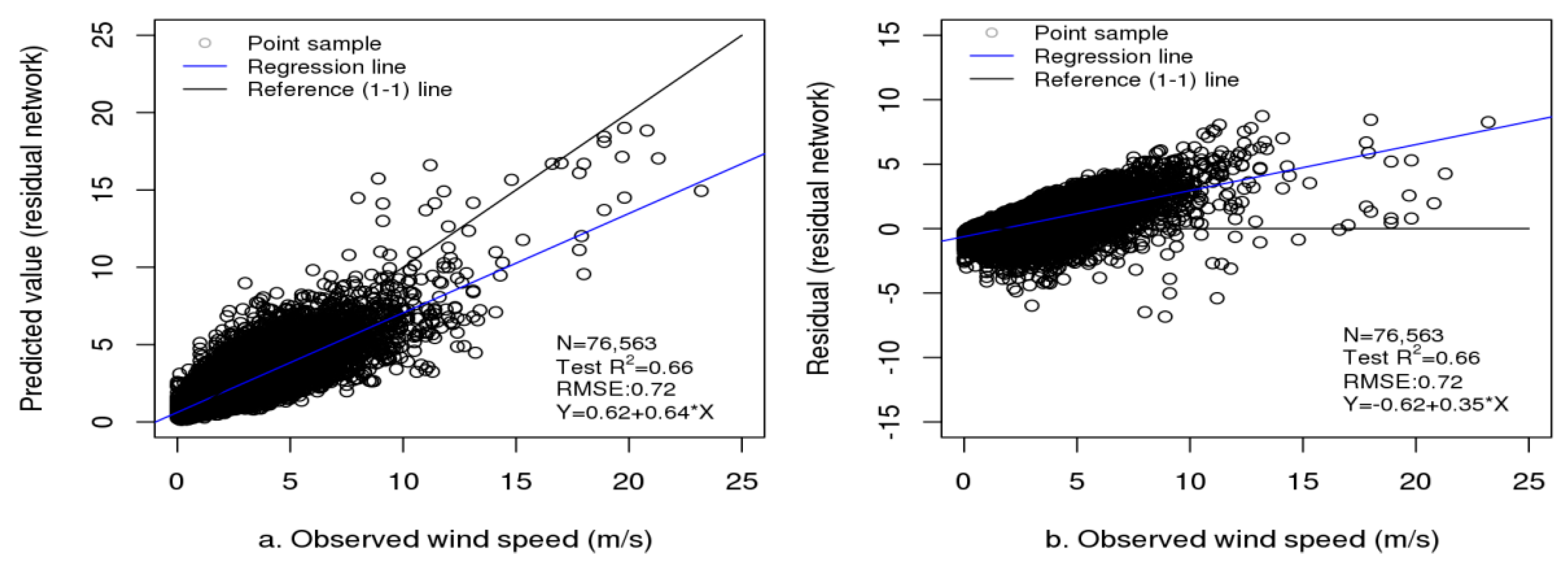
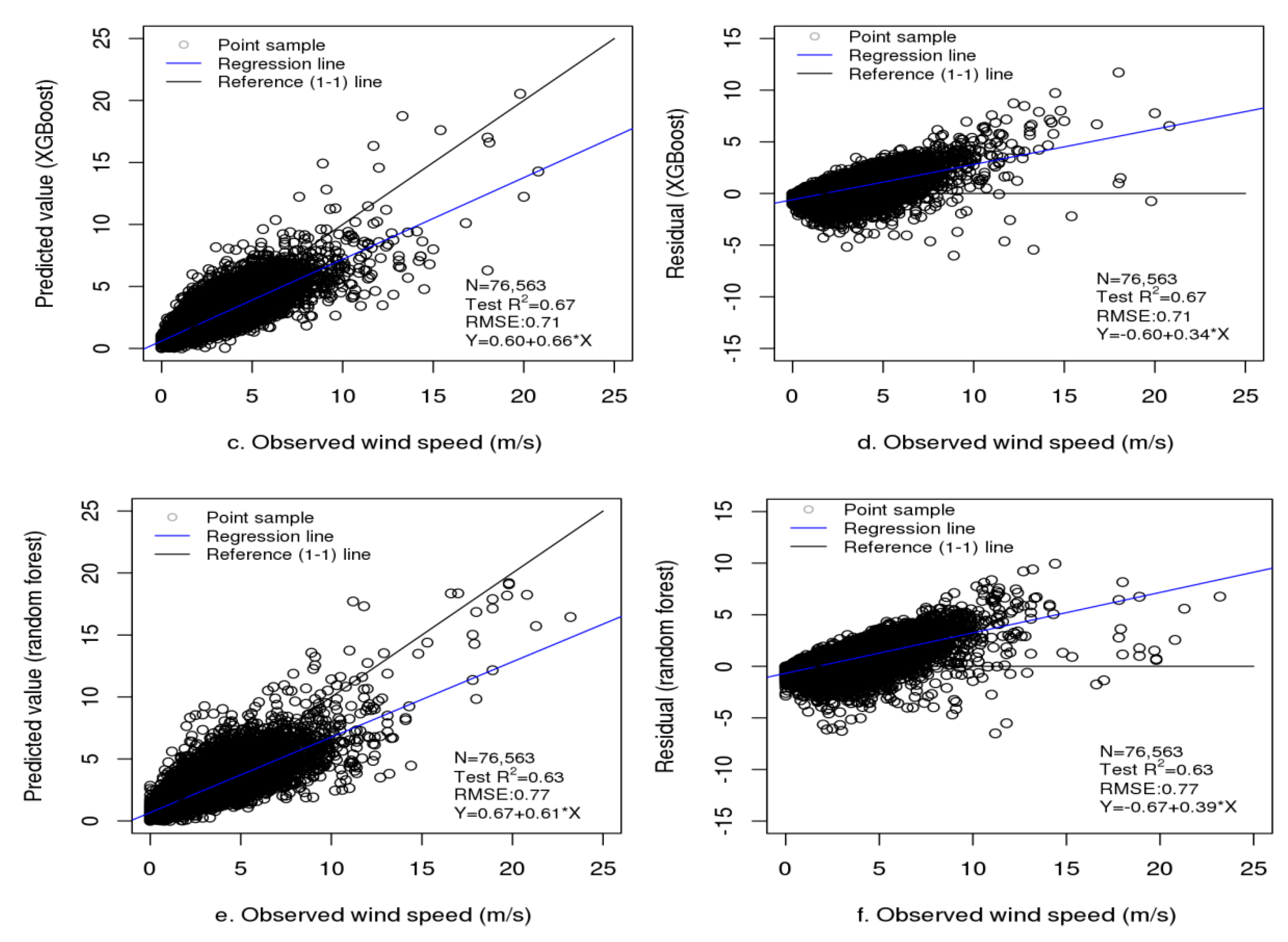
In Stage 1, each of the three individual models was trained, and then, their predictions were geographically weighted to obtain the ensemble predictions. Table 2 presents the performances of the three base models, GAM and the feed-forward neural network in training and independent tests. In total, 76,563 independent test samples were obtained. The autoencoder-based deep network had a training R2 of 0.68 (training RMSE: 0.76 m/s) (RMSE represents the error), which was lower than the training R2 (0.76) of XGBoost (RMSE: 0.60 m/s) and slightly lower than the training R2 (0.69) of random forest (RMSE: 0.76 m/s). However, the three models had similar independent test R2 and RMSE values with very slight differences (test R2: 0.66 for residual network, 0.67 for XGBoost and 0.63 for random forest; test RMSE: 0.72 m/s for residual network, 0.71 m/s for XGBoost and 0.77 m/s for random forest). The result shows much higher test R2 (0.63–0.67 vs. 0.42–0.58), and lower test RMSE (0.71–0.77 m/s vs. 0.82–0.96 m/s) and MAE (0.51–0.53 vs. 0.57–0.67) for the deep residual network, XGBoost and random forest than GAM and the feed-forward neural network. Figure 6 shows faster convergence with lower loss and higher validation R2 for deep residual network than for feed-forward neural network. The results also show a lower difference in R2 and RMSE between the training and testing for autoencoder-based deep residual networks, indicating less overfitting in generalization. Figure 7 shows the plots of the predicted values/residuals against the observed values for the three individual wind speed models. In terms of their generalizations in independent tests, the three individual models had similar performance with very slight differences.
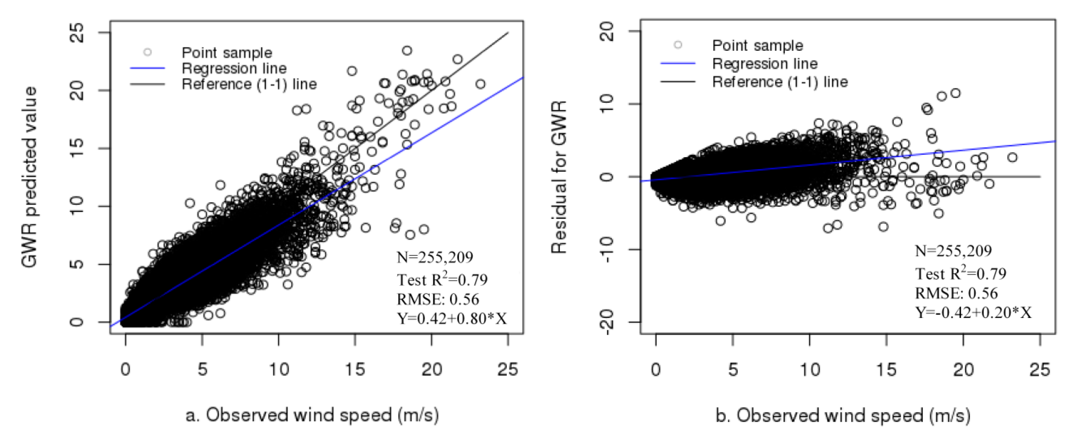
In the ensemble machine learning by GWR, the ensemble predictions had a test R2 of 0.79 with a test RMSE of 0.58 m/s (training R2: 0.81; training RMSE of 0.56 m/s) (see Supplementary Materials Figure S2 for boxplots of their observed and predicted values). The their observed values plotted against predicted values and residuals in the test are shown in Figure 8. The results show that the test R2 improved by 12-16% over individual models and that the test RMSE decreased by 0.14-0.19 m/s. The results show a considerable contribution of GWR to the ensemble predictions by accounting for spatial autocorrelation and heterogeneity. In the GWR test, Moran’s I was obtained for the residuals of each day of 2015. The results showed no spatial autocorrelation (with p-value ≥ 0.05 indicating that null hypothesis of complete spatial randomness cannot be refused) or low Moran’s I (mean: 0.06; range: 0.001–0.15), indicating very weak spatial correlation. Additionally, the variogram of exponential models was selected through sensitivity analysis and fitted. The results of four typical days (spring: 1 April 2015; summer: 1 July 2015; autumn: 1 October 2015; winter: 20 December 2015) are presented in Supplementary Materials Table S1 for optimal parameters of the variogram models, and LOOCV R2 and RMSE between original residuals and estimated residuals by universal kriging, as well as Supplementary Materials Figures S3 and S4 for the plots of variogram and scatter points between original and estimated residuals, respectively. Very small LOOCV R2 (negative values) and almost random patterns of the scatter plots showed little contribution of variogram based universal kriging to estimation of the residuals.
4.3. Predictions and Downscaling in Stage 2
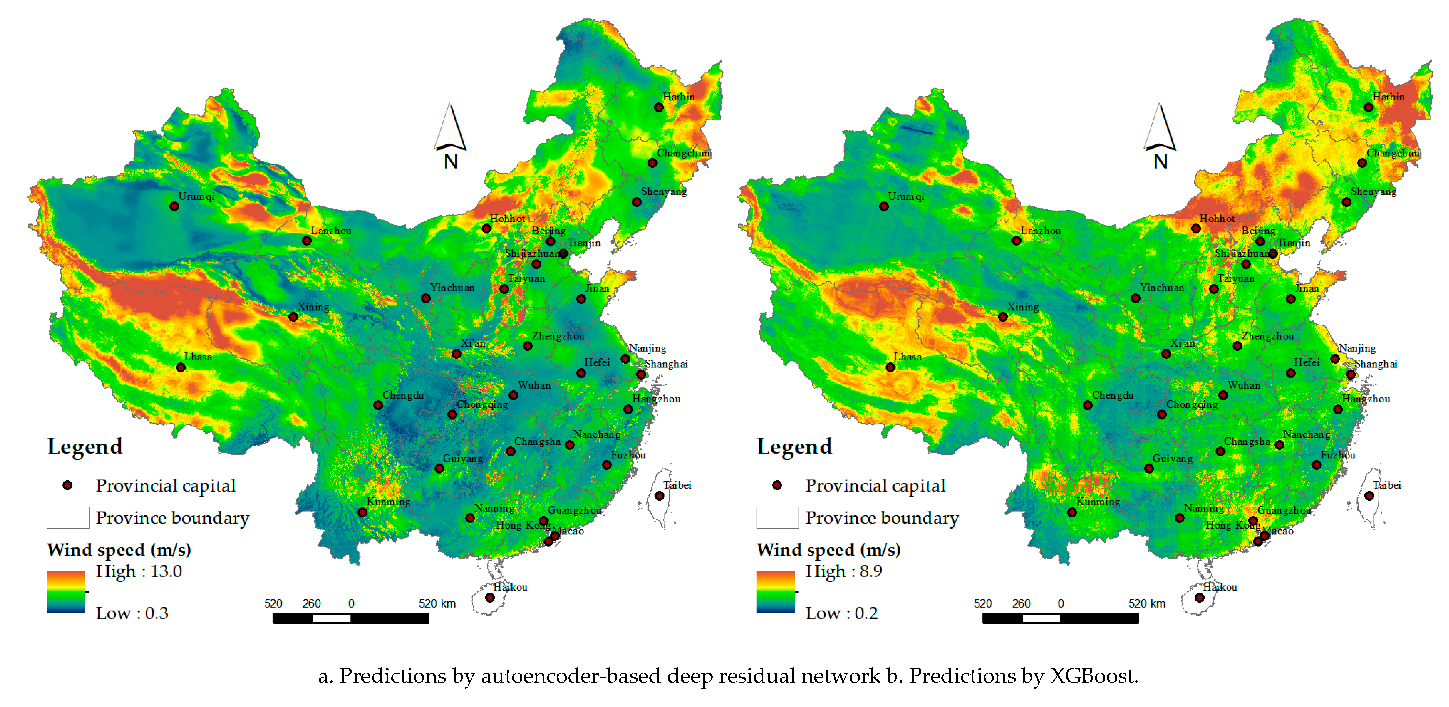
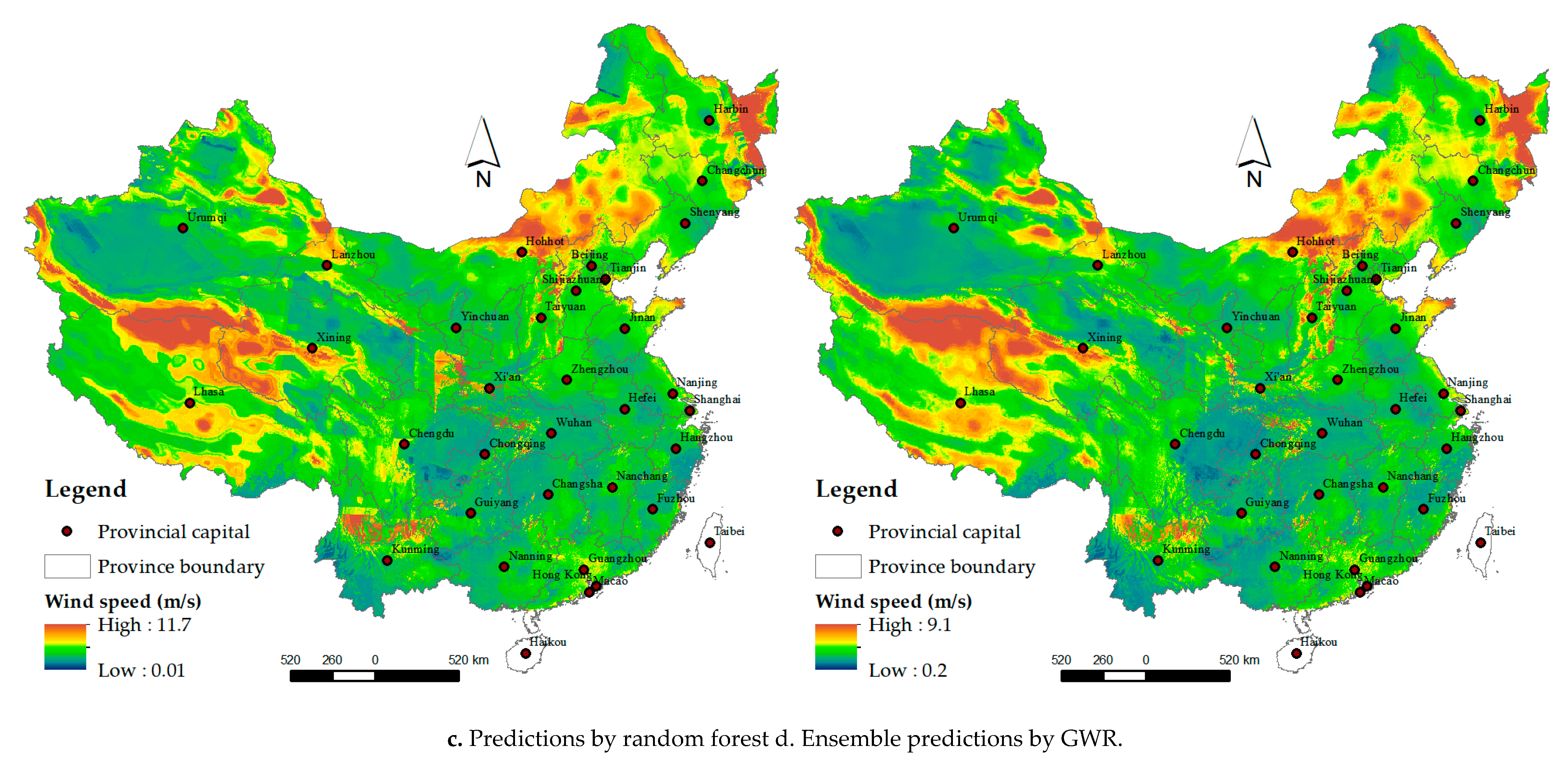
With the models trained in Stage 1, the daily wind speed was predicted (spatial resolution: 1 km) for 2015 in mainland China. Figure 9 shows the prediction grids of a typical day (1 January 2015) in winter for the three individual learners and GWR (a for the autoencoder-based deep network, b for XGBoost, c for random forest and d for ensemble predictions by GWR). For the purpose of comparison, this paper also shows the prediction grids of a typical day (1 July 2015) in summer in Supplementary Materials Figure S5. For ensemble predictions, spatially varying coefficients for the intercept and the coefficients for the predictors were obtained as the GWR output for 1 January 2015 (Supplementary Materials Figure S6). The results show positive effects for XGBoost in northwestern and southern China and for random forest in central and eastern China and negative effects for the deep residual network in midwestern and northeastern China, for XGBoost in central and northeastern China, and for random forest in northwestern China. The variance grids of the ensemble predictions for 1 January 2015 by GWR were also obtained (Supplementary Materials Figure S7) as an indicator of the uncertainty. The results showed higher variance at several locations in western and northeastern China than that in other regions.
As shown in b and c of Figure 9 and Supplementary Materials Figure S5, even with a similar test performance, the prediction grids using XGBoost and random forest are fine overall but show some spatial abrupt (non-natural) variation on a local scale, possibly due to the discretization of the features in the decision/regression trees used as base models in XGBoost and random forest. Comparatively, the prediction grids produced by the autoencoder-based deep residual network appear naturally spatially smooth. Furthermore, the ensemble predictions from the three learners generated by GWR reduced the spatial abrupt variation, as shown in d of the two figures.
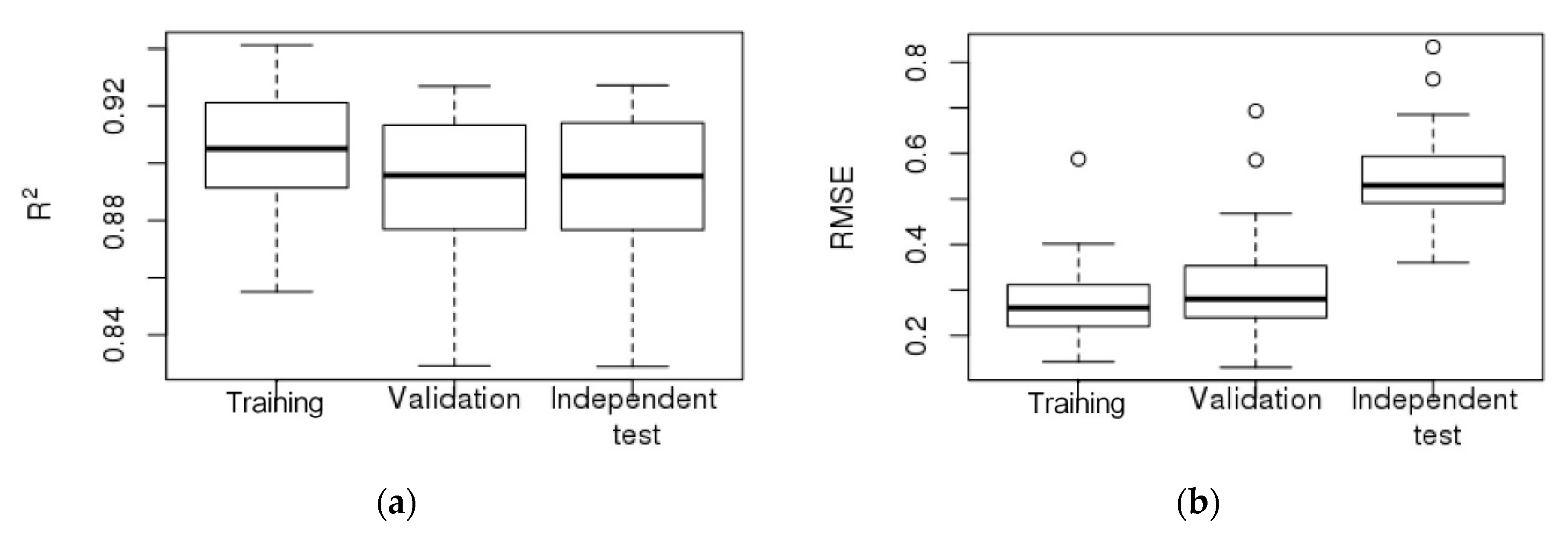
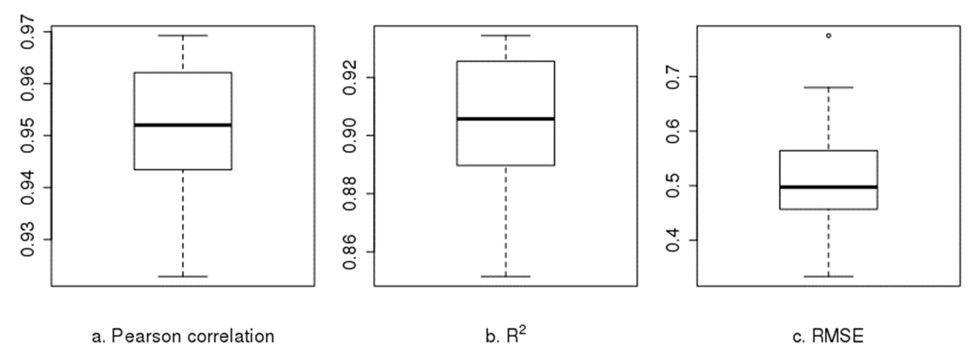
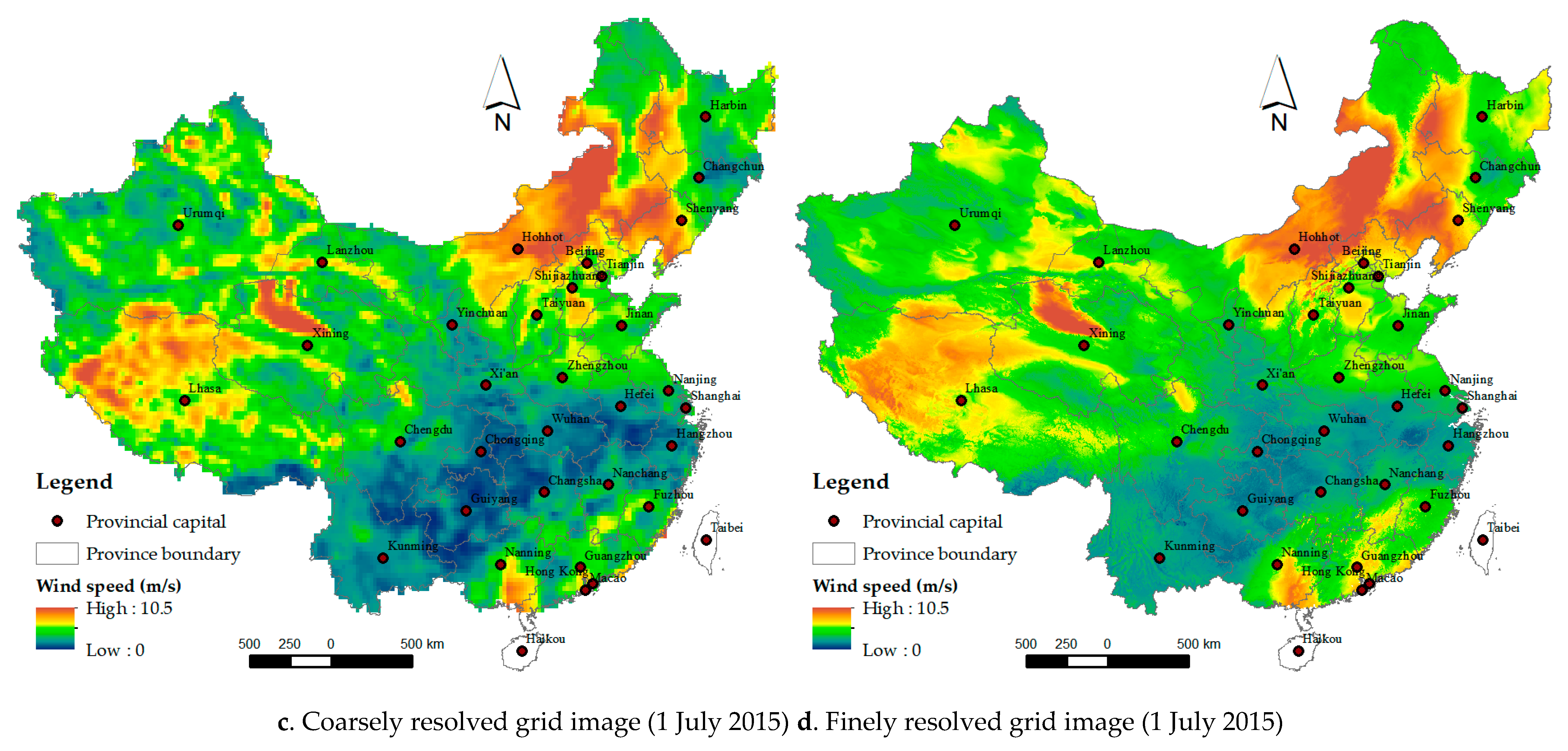
In Stage 2 downscaling, the deep residual network regressed the 2015 daily finely resolved grid cells over the covariates, with the regularizer of their averages equal to the coarsely resolved grid cell (Figure 10): test R2: mean of 0.89 with a range from 0.83 to 0.93; test RMSE: mean of 0.54 m/s with a range from 0.36 m/s to 0.83 m/s. The coarsely resolved grid cells and the corresponding averages of the predicted finely resolved grid cells both matched statistically for 2015 (Figure 11): Pearson correlation: mean of 0.95 with a range from 0.92 to 0.97; R2: mean of 0.91 with a range from 0.85 to 0.93; RMSE: mean of 0.51 m/s with a range from 0.33 m/s to 0.78 m/s. The plots (Supplementary Materials Figure S8) of the average finely resolved wind speed within each coarsely resolved grid cell and their residuals against the coarsely resolved wind speed (reanalysis data) for 1 January 2015 and 1 July 2015 show a close match between both with few outliers. The final finely and original coarsely resolved images for the two dates are shown in Figure 12.
Time series of daily finely resolved grids of wind speed for 2015 were made across mainland China. Figure 13 shows four typical days of 2015, as aforementioned. Overall, high wind speeds were more evenly distributed across mainland China in spring and summer than in autumn and winter. On average, spring, summer and autumn had higher wind speeds than winter. In winter, the locations in and close to the Tibet region of western China had higher wind speeds than those in other regions. The low wind speed aggravated air pollution in the Beijing-Tianjin-Hebei region [47].
5. Discussion
This paper proposes a two-stage approach for the robust estimation of wind speed, which is known to be challenging due to complex influential factors and wind speed volatility. In the proposed approach, Stage 1 aims to improve reliable estimates of the target variable to capture contrast or spatiotemporal variability at a fine resolution using geographically weighted machine learning, and Stage 2 aims to adjust the finely resolved prediction grids initially inferred from Stage 1 to make them consistent with the coarsely resolved reanalysis data. Stage 2 reduced overfitting and improved spatial variation (smoothing). Therefore, the proposed approach can obtain reliable high-resolution wind speed estimations.
High-resolution mapping of meteorological parameters is challenging due to the limited number of available covariates (e.g., just nine covariates in the case of this paper), as multiple factors affect spatiotemporal variability and they present complex interactions. Although meteorological reanalysis employs comprehensive data from a variety of sources, including ground-based stations, ships, airplanes, satellites, and forecasts from numerical weather prediction models, to estimate meteorological parameters in the state of the system as accurately as possible [24], their spatial resolution is very coarse, thus constraining their applicability at local levels. Considering this challenge, in Stage 1, a geographically weighted machine learning method was adopted based on three representative state-of-the-art learners: an autoencoder-based deep residual network, XGBoost and random forest. In comparison with GAM and the feed-forward neural network, the test showed that the three base learners achieved much better generalization and efficient learning. Compared with support vector machine (SVM) and the fuzzy neural system, which presented very slow convergence in the test using the wind speed samples, the three learners were convenient to use, with high generalization and fewer feature engineering operations.
Although these learners achieved good performance with spatial autocorrelation partially captured by the coordinates and their derivatives, spatial autocorrelation was not embedded directly within the models, and thus their residuals might present spatial autocorrelation. Furthermore, for large regions such as mainland China, there is considerable diversity and many differences exist between regions. Therefore, geographically weighted machine learning was leveraged to integrate the predictions made by the three types of learners. As a local regression technique, GWR was used to account for spatial autocorrelation and heterogeneity [48,49,50], compensating for the shortcomings of modern machine learners to improve ensemble predictions. In the test of the 2005 wind speed for mainland China, individual learners achieved an R2 of 0.63–0.67 (RMSE: 0.72–0.77 m/s) in independent tests, and GWR further improved the R2 to 0.79 (RMSE: 0.58 m/s) in LOOCV. The results showed that GWR effectively improved the predictions of individual learners by spatially varying fusion. The results of very small Moran’s I in the residuals of ensemble predictions and little contribution of variogram-based universal kriging to estimation of the residuals illustrated that most of the spatial autocorrelation was accounted for by the proposed approach.
Due to the discretization of the quantitative covariates used in the decision (regression) trees, massive grid predictions by the decision tree-based methods [51] (XGBoost and random forest) might present spatial abrupt (non-natural) variation at the local spatial scale, as shown in Figure 9. Comparatively, the autoencoder-based deep residual network did not involve discretization of covariates whose fully continuous quantitative information was kept in the models and thus could generate prediction grids with spatially smoother surfaces than XGBoost and random forest. Then, the ensemble predictions from the three base models were fused using GWR, which mitigated the spatial abrupt variation. Therefore, using three individual robust learners and GWR, the ensemble estimates can effectively capture the contrast or variability of the target variable at a fine spatial scale with improved R2 and lower RMSE.
To further reduce the potential bias and improve spatial variation (smoothing) of predicted values (caused by decision tree-based algorithms), coarsely resolved reanalysis data, if reliable, can be used as the regularizer to adjust the ensemble estimates to make them consistent with the coarse-resolution grids at the background scale. To achieve reliable generalization with complete removal of spatial abrupt (non-natural) variation, an autoencoder-based deep residual network was used to regress the adjusted or regularized ensemble outputs over the selected covariates. Therefore, the specific contrast or variability at fine resolution captured in Stage 1 could be kept in downscaling with the reliable coarsely resolved reanalysis data to obtain reasonable grids. The example of wind speed illustrated effective simulation in downscaling to reduce bias and improve spatial variation (smoothing). The downscaled time series of the finely resolved grids presented reasonable seasonal patterns of wind speed across mainland China.
For downscaling, compared with kriging-based ATPP interpolation [25], autoencoder-based deep residual network provides a flexible network architecture with a large parameter space. Although spatial autocorrelation, such as kriging, was not directly embedded in the network, GWR was used to capture spatial autocorrelation and heterogeneity in Stage 1 at a local fine scale. Furthermore, coordinates and their interaction derivatives were used as covariates within the model to represent spatial variation in Stage 2 downscaling. In contrast to the kriging method, the downscaling of the deep residual network did not require variogram simulation, which might introduce uncertainty for the volatile wind speed. Sensitivity analysis showed that the universal kriging accounted for only 14% of the variance explained for wind speed (but 72% for relative humidity), compared to 66% by the autoencoder-based deep residual network in the independent test. This illustrated the inapplicability of kriging interpolation for capturing the variability of mutable wind speed, and showed that the proposed approach can better predict wind speed.
For application to other meteorological or surface variables and other regions, this proposed approach is divided into two stages (Figure 2). Stage 1 aims to train three base learners (deep residual network, XGBoost and random forest) and GWR using X and y from the training samples. Stage 2 involves inference (prediction) and downscaling using the new and reanalysis datasets to obtain reliable high-resolution grid predictions. The new dataset first supplied X to the trained base learners and GWR in Stage 1 to get the initial finely resolved predictions, . Then, the coarse-resolution reanalysis data were used to adjust or (inferred by the downscaling model in each iteration). Then, X and adjusted or were used to train or retrain the downscaling model. This process was repeated until the preselected stopping criterion value (SCV) was attained, as shown in Figure 5.
This study has the following limitations. First, although downscaling was introduced in Stage 2 with coarsely resolved reanalysis data to adjust the ensemble predictions, the reanalysis data were assumed to be reliable so that the adjusted surfaces in downscaling could also be reliable. Otherwise, downscaling may distort the adjusted outcomes and evenly introduce bias into the results. Second, the proposed approach did not embed the mechanism knowledge for generating wind speed within the models, but instead used only a limited number of available covariates to capture spatiotemporal variability in Stage 1. However, the coarse-resolution reanalysis data were also used as the covariates within the model that represent hybrid results based on climate models, numeric predictions, satellite data and monitoring data. In particular, downscaling with the coarse-resolution reanalysis data was introduced to regularize the ensemble results. Third, the wind speed data used to train the models were primarily measured at a height of 10–12 m above the ground and thus the trained models predicted wind speed at a similar height. This may limit the application of the results for recovery of the wind potential for energy purposes, which involves estimating the wind speed at heights between 50–100 m above the ground. However, this paper focused on machine learning methods for high spatiotemporal mapping of wind speed rather than practical applications of wind potential recovery. Regarding the latter, new measurement data of wind speed may be gathered to retrain the models for an appropriate evaluation of wind potential.
6. Conclusions
In this study, a two-stage approach was developed to make robust high-resolution wind speed predictions across a large region, such as mainland China. In the proposed approach, Stage 1 obtained geographically weighted ensemble predictions based on three different types of robust learners, which were an autoencoder-based deep residual network, XGBoost and random forest, to capture spatiotemporal contrast or variability at fine resolutions with improved performance. Stage 2 introduced downscaling using the coarsely resolved reanalysis data as a regularizer to make the coarsely resolved grids and the averages of the overlaid finely resolved grids consistent. In the case study of wind speed prediction for mainland China, the proposed approach achieved a CV R2 of 0.79 (RMSE: 0.58 m/s) in GWR ensemble predictions and a mean R2 of 0.91 for the 2015 daily match of coarsely and finely resolved grids in downscaling. This approach provides reliable and robust predictions for wind speed and can be applied for high-resolution spatiotemporal estimation of other meteorological parameters and surface variables that involve multiple influential factors at different scales.
Supplementary Materials
The following are available online at https://0-www-mdpi-com.brum.beds.ac.uk/2072-4292/11/11/1378/s1: Table S1: Variogram fitting and cross validation for estimation of the residuals of predicted wind speed for four typical seasonal days (b); Figure S1: Histograms for wind speed (a) and its log transformations (b); Figure S2: Boxplots of the observed values and ensemble predictions by GWR for wind speed; Figure S3: Plots of variogram fitting; Figure S4: Plots of the original residual from ensemble predicted wind speed vs. estimated residuals using fitted variogram based universal kriging (UK) for four typical seasonal days; Figure S5: Predictions by individual models (a for autoencoder-based deep network, b for XGBoost and c for random forest) and their ensemble predictions by GWR for wind speed of 1 July 2015; Figure S6: Spatially varying intercept (a) and coefficients (b, c and d) for the predictions of thee individual learners for wind speed; Figure S7: Spatially varying variance for the ensemble predictions by GWR for wind speed; Figure S8: Plots of averages of matched finely resolved wind speed (a and c) and their residuals (b and d) vs. the coarsely resolved wind speed (reanalysis data) for 1 January 2015 (a and b) and 1 July 2015 (c and d).
Author Contributions
L.L. was responsible for conceptualization, methodology, software, validation, formal analysis and writing.
Funding
This work was supported in part by the Strategic Priority Research Program of Chinese Academy of Sciences Grant XDA19040501 and in part by the National Natural Science Foundation of China under Grant 41471376.
Acknowledgments
The support of NVIDIA Corporation with the donation of the Titan Xp GPUs used for this research and Ms. Ying Fang’s support for this study are gratefully acknowledged.
Conflicts of Interest
The author declares no conflict of interest.
References
- Hewson, E.W. Meteorological Factors Affecting Causes and Controls of Air Pollutio. J. Air Pollut. Control Assoc. 1956, 5, 235–241. [Google Scholar] [CrossRef]
- National Research Council. Coastal Meteorology: A Review of the State of the Science; The National Academies Press: Washington, DC, USA, 1992. [Google Scholar]
- Puc, M.; Bosiacka, B. Effects of Meteorological Factors and Air Pollution on Urban Pollen Concentrations. Pol. J. Environ. Stud. 2011, 20, 611–618. [Google Scholar]
- Bohnenstengel, I.S.; Belcher, E.S.; Aiken, A. Meteorology, Air Quality, and Health in London: The ClearfLo Project. Am. Meteorol. Soc. 2015, 779–804. [Google Scholar] [CrossRef]
- Scorer, R.R. Air Pollution Meteorology; Woodhead Publishing: Cambridge, UK, 2002. [Google Scholar]
- Jhun, I.; Coull, B.A.; Schwartz, J.; Hubbell, B.; Koutrakis, P. The impact of weather changes on air quality and health in the United States in 1994–2012. Environ. Res. Lett. 2015, 10, 084009. [Google Scholar] [CrossRef]
- WHO. Extreme Weather and Climate Events and Public Health Response; European Environment Agency: Bratislava, Slovakia, 2004. [Google Scholar]
- Ronay, A.K.; Fink, O.; Zio, E. Two Machine Learning Approaches for Short-Term Wind Speed Time-Series Prediction. IEEE Trans. Neural Netw. Learn. Syst. 2016, 27, 1734–1747. [Google Scholar]
- Dee, P.E.; Uppala, M.S.; Simmons, J.A. The ERA-Interim reanalysis: Configuration and performance of the data assimilation system. Q. J. R. Meteorol. Soc. 2011, 137, 5697. [Google Scholar] [CrossRef]
- Rienecker, M.M.; Suarez, J.M.; Gelaro, R. MERRA—NASA’s Modern-Era Retrospective Analysis for Research and Applications. J. Clim. 2011, 24, 3624–3648. [Google Scholar] [CrossRef]
- Saha, S.; Moorthi, S.; Pan, H.; Wu, X. The NCEP Climate Forecast System Reanalysis. Bull. Am. Meteorol. Soc. 2010, 91, 1015–1057. [Google Scholar] [CrossRef]
- Cai, Q.; Wang, W.; Wang, S. Multiple Regression Model Based on Weather Factors for Predicting the Heat Load of a District Heating System in Dalian, China—A Case Study. Open Cybern. Syst. J. 2015, 9, 2755–2773. [Google Scholar] [CrossRef]
- Jie, H.; Houjin, H.; Mengxue, Y.; Wei, Q.; Jie, X. A time series analysis of meteorological factors and hospital outpatient admissions for cardiovascular disease in the Northern district of Guizhou Province, China. Braz. J. Med. Biol. Res. 2014, 47, 689–696. [Google Scholar] [CrossRef] [Green Version]
- Voet, P.; Diepen, C.; Voshaar, J.O. Spatial Interpolation of Daily Meteorological Data; DLO Winand Starting Center: Wageningen, The Netherlands, 1995. [Google Scholar]
- Yang, G.; Zhang, J.; Yang, Y.; You, Z. Comparison of interpolation methods for typical meteorological factors based on GIS—A case study in Jitai basin, China. In Proceedings of the 19th International Conference on Geoinformatics, Shanghai, China, 24–26 June 2011. [Google Scholar]
- Wiki. Climate Model. Wikimedia Foundation, Inc., 2018. Available online: https://en.wikipedia.org/wiki/Climate_model (accessed on 9 June 2019).
- Mohandes, M.; Halawani, O.T.; Rehman, S.; Hussain, A.A. Support vector machines for wind speed prediction. Renew. Energy 2004, 29, 939–947. [Google Scholar] [CrossRef]
- Lei, M.; Shiyan, L.; Chuanwen, J.; Hongling, J.; Yan, Z. A review on the forecasting of wind speed and generated power. Renew. Sustain. Energy Rev. 2009, 13, 915–920. [Google Scholar] [CrossRef]
- Philippopoulos, K.; Deligiorgi, D.; Kouroupetroglou, G. Artificial Neural Network Modeling of Relative Humidity and Air Temperature Spatial and Temporal Distributions Over Complex Terrains. In Pattern Recognition Applications and Methods; Basel, Springer: Switzerland, 2014; pp. 171–187. [Google Scholar]
- Traiteur, J.J.; Callicutt, J.D.; Smith, M.; Roy, B.S. A Short-Term Ensemble Wind Speed Forecasting System for Wind Power Applications. Am. Meteorol. Soc. 2012, 1763–1774. [Google Scholar] [CrossRef]
- Jones, N. How machine learning could help to improve climate forecasts. Nature 2017, 584, 379–380. [Google Scholar] [CrossRef]
- Bishop, M.C. Neural Networks for Pattern Recognition; Oxford University Press: Oxford, UK, 1995. [Google Scholar]
- Goodfellow, I.; Bengio, Y.; Courville, A. Deep Learning; MIT Press: Cambridge, MA, USA, 2016. [Google Scholar]
- Parker, W. Reanalyses and observations, what is the difference? Am. Meteorol. Soc. 2016. [Google Scholar] [CrossRef]
- Atkinson, M.P. Downscaling in remote sensing. Int. J. Appl. Earth Obs. Geoinf. 2012, 22, 106–114. [Google Scholar] [CrossRef]
- Gotway, C.A.; Young, L.J. Combining incompatible spatial data. J. Am. Stat. Assoc. 2002, 97, 632–648. [Google Scholar] [CrossRef]
- Goovaerts, P. Combining areal and point data in geostatistical interpolation: Applications to soil science and medical geography. Math. Geosci. 2010, 42, 535–554. [Google Scholar] [CrossRef]
- Pardo-Iguzquiza, E.; Rodriguez-Galiano, V.F.; Chica-Olmo, M.; Atkinson, P.M. Image fusion by spatially adaptive filtering using downscaling cokriging. ISPRS J. Photogramm. Remote Sens. 2011, 66, 337–346. [Google Scholar] [CrossRef]
- Li, L.; Fang, Y.; Wu, J.; Wang, J. Autoencoder Based Residual Deep Networks for Robust Regression Prediction and Spatiotemporal Estimation. arXiv 2018, arXiv:1812.11262. [Google Scholar]
- Rovithakis, A.G.; Christodoulou, A.M. Adaptive control of unknown plants using dynamical neural networks. IEEE Trans. Syst. Man Cybern. 1994, 24, 400–412. [Google Scholar] [CrossRef]
- Yu, W. PID Control with Intelligent Compensation for Exoskeleton Robots; Elsevier Inc.: Amsterdam, The Netherlands, 2018. [Google Scholar]
- Wiki. Planetary Boundary Layer. Wikimedia Foundation, Inc., 2018. Available online: https://en.wikipedia.org/wiki/Planetary_boundary_layer (accessed on 9 June 2019).
- Wizelius, T. The relation between wind speed and height is called the wind profile or wind gradient. In Developing Wind Power Projects; Earthscan Publications Ltd.: London, UK, 2007; p. 40. [Google Scholar]
- Chen, T.; Guestrin, C. XGBoost: A Scalable Tree Boosting System. arXiv 2016, arXiv:1603.02754. [Google Scholar]
- Ho, T.K. The Random Subspace Method for Constructing Decision Forests. IEEE Trans. Pattern Anal. Mach. Intell. 1998, 20, 832–844. [Google Scholar]
- Hastie, T.; Tibshirani, R.; Friedman, J. The Elements of Statistical Learning, 2nd ed.; Springer: Berlin, Germany, 2008. [Google Scholar]
- He, K.M.; Zhang, X.Y.; Ren, S.Q.; Sun, J. Identity Mappings in Deep Residual Networks. Lect. Notes Comput. Sci. 2016, 9908, 630–645. [Google Scholar]
- Srivastava, K.R.; Greff, K.; Schmidhuber, J. Highway networks. arXiv 2015, arXiv:1505.00387. [Google Scholar]
- He, K.; Sun, J. Convolutional neural networks at constrained time cost. arXiv 2015, arXiv:1603.02754. [Google Scholar]
- He, K.M.; Zhang, X.Y.; Ren, S.Q.; Sun, J. Deep Residual Learning for Image Recognition. In Proceedings of the 2016 IEEE Conference on Computer Vision and Pattern Recognition (CVPR), Las Vegas, NV, USA, 27–30 June 2016; pp. 770–778. [Google Scholar]
- Zou, H.; Hastie, T. Regularization and Variable Selection via the Elastic Net. J. R. Stat. Soc. Ser. B 2005, 67, 301–320. [Google Scholar] [CrossRef]
- Breiman, L. Random forests. Mach. Learn. 2001, 45, 5–32. [Google Scholar] [CrossRef]
- Fotheringham, A.; Charlton, M. Geographically weighted regression: A natural evolution of the expansion method for spatial data analysis. Environ. Plan. A 1998, 30, 1905–1927. [Google Scholar] [CrossRef]
- Tobler, W. A computer movie simulating urban growth in the Detroit region. Econ. Geogr. 1970, 46, 234–240. [Google Scholar] [CrossRef]
- Li, H.; Calder, C.; Cressie, N. Beyond Moran’s I. Testing for Spatial Dependence Based on the Spatial Autoregressive Model. Geogr. Anal. 2007, 39, 357–375. [Google Scholar] [CrossRef]
- Iglewicz, B.; Hoaglin, C.D. How to Detect and Handle Outliers. In The ASQ Basic References in Quality Control: Statistical Techniques; Mykytka, F.E., Ed.; American Society for Quality: Milwaukee, WI, USA, 1993. [Google Scholar]
- Zou, Y.; Wang, Y.; Zhang, Y.; Koo, J. Arctic sea ice, Eurasia snow, and extreme winter haze in China. Sci. Adv. 2017, 3, 1–9. [Google Scholar] [CrossRef]
- Charlton, M.; Fotheringham, S. Geographically Weighted Regression A Tutorial on Using GWR in ArcGIS 9.3; National Centre for Geocomputation National University of Ireland: County Kildare, Ireland, 2018. [Google Scholar]
- Lu, B.; Charlton, M.; Harris, P.; Fotheringham, S. Geographically weighted regression with a non-Euclidean distancemetric: A case study using hedonic house price data. Int. J. Geogr. Inf. Sci. 2014, 28, 660–681. [Google Scholar] [CrossRef]
- Propastin, P.; Kappas, M.; Erasmi, S. Application of geographically weighted regression to investigate the impact of scale on prediction uncertainty by modelling relationship between vegetation and climate. Int. J. Spat. Data Infrastruct. Res. 2008, 3, 73–94. [Google Scholar]
- Rokach, L.; Maimon, O. Data Mining with Decision Trees: Theory and Applications; World Scientific Pub. Co. Inc.: Danvers, MA, USA, 2008. [Google Scholar]
Figure 1.
Study region of China’s mainland with monitoring stations of wind speed.

Figure 2.
Systematic framework: training of base models and geographically weighted regression (GWR) (Stage 1) and inference and downscaling (Stage 2).
Figure 2.
Systematic framework: training of base models and geographically weighted regression (GWR) (Stage 1) and inference and downscaling (Stage 2).

Figure 3.
Geographically weighted ensemble machine learning.

Figure 4.
Autoencoder-based deep residual network for wind speed (9 input variables).

Figure 5.
Downscaling algorithm by autoencoder-based deep residual network.

Figure 6.
Learning curves (a. validation loss; b. validation R2) of deep residual network vs. feed- forward neural network.
Figure 6.
Learning curves (a. validation loss; b. validation R2) of deep residual network vs. feed- forward neural network.

Figure 7.
Plots of observed values (a,c,e) and residuals (b,d,f) vs. predicted values of wind speed for autoencoder-based residual network (a,b), XGBoost (c,d) and random forest (e,f) for the independent tests.
Figure 7.
Plots of observed values (a,c,e) and residuals (b,d,f) vs. predicted values of wind speed for autoencoder-based residual network (a,b), XGBoost (c,d) and random forest (e,f) for the independent tests.


Figure 8.
Observed vs. predicted values (a) and residual (b) plots of wind speed in the test.

Figure 9.
Predictions at a height of 10–12 m above the ground by individual models (a) for autoencoder-based deep residual network, (b) for XGBoost and (c) for random forest) and their ensemble predictions by GWR (d) for wind speed of 1 January 2015.
Figure 9.
Predictions at a height of 10–12 m above the ground by individual models (a) for autoencoder-based deep residual network, (b) for XGBoost and (c) for random forest) and their ensemble predictions by GWR (d) for wind speed of 1 January 2015.


Figure 10.
Statistical boxplot for the performance (training, validation and test R2 (a) and RMSE (b) of the deep residual network in downscaling using meteorological reanalysis data.
Figure 10.
Statistical boxplot for the performance (training, validation and test R2 (a) and RMSE (b) of the deep residual network in downscaling using meteorological reanalysis data.

Figure 11.
Boxplots of correlation (a), R2 (b) and RMSE (c) between the averages of finely resolved grid cells (predicted) and the corresponding coarsely resolved grid cells (reanalysis data).
Figure 11.
Boxplots of correlation (a), R2 (b) and RMSE (c) between the averages of finely resolved grid cells (predicted) and the corresponding coarsely resolved grid cells (reanalysis data).

Figure 12.
Adjusted wind speed image at a height of 10–12 m above the ground (b,d) by downscaling of deep residual network and their original coarsely resolved image (a,c) for 1 January 2015 (a,b) in winter and 1 July 2015 (c,d) in summer.
Figure 12.
Adjusted wind speed image at a height of 10–12 m above the ground (b,d) by downscaling of deep residual network and their original coarsely resolved image (a,c) for 1 January 2015 (a,b) in winter and 1 July 2015 (c,d) in summer.


Figure 13.
High spatial-resolution maps of wind speed at a height of 10–12 m above the ground for a typical day in each of the four seasons of 2015 in China’s mainland.
Figure 13.
High spatial-resolution maps of wind speed at a height of 10–12 m above the ground for a typical day in each of the four seasons of 2015 in China’s mainland.


Table 1.
Statistics for the measurements and the covariates for the sample data of wind speed.
| Item | WSa | WSIb | O3Ic | PBLHd | TEMIe | ELEf |
|---|---|---|---|---|---|---|
| Unit | m/s | m/s | DU | m | °C | m |
| Mean | 2.1 | 2.8 | 318.6 | 683.4 | 12.9 | 790.2 |
| Median | 1.8 | 2.4 | 311.9 | 612.3 | 13.3 | 400.0 |
| IQR | 1.4 | 1.9 | 52.3 | 531.0 | 16.6 | 1045.5 |
| Range | 0.0, 23.2 | 0.3, 19.2 | 219.4, 484.4 | 55.7, 3865.8 | −18.1, 38.4 | 1.8, 4800.0 |
Note: WSa: wind speed; WSIb: wind speed of reanalysis data; O3Ic: ozone concentrations of reanalysis data; PBLHd: planetary boundary layer height of reanalysis data; TEMIe: surface temperature of reanalysis data; ELEf: elevation of the Shuttle Radar Topology Mission (SRTM).
Table 2.
Performances of individual models.
| Base Model | Training | Independent Test | ||||||
|---|---|---|---|---|---|---|---|---|
| R2 | Adjusted R2 | RMSEa | MAEb | R2 | Adjusted R2 | RMSE | MAE | |
| ARNc | 0.68 | 0.68 | 0.76 | 0.49 | 0.66 | 0.66 | 0.72 | 0.51 |
| XGBoost | 0.76 | 0.76 | 0.60 | 0.46 | 0.67 | 0.67 | 0.71 | 0.51 |
| RFd | 0.69 | 0.69 | 0.76 | 0.49 | 0.63 | 0.63 | 0.77 | 0.53 |
| GAMe | 0.43 | 0.43 | 0.95 | 0.67 | 0.42 | 0.42 | 0.96 | 0.67 |
| FFNNf | 0.58 | 0.58 | 0.83 | 0.57 | 0.58 | 0.58 | 0.82 | 0.57 |
Note: RMSEa: root mean square error; RAEb: mean absolute error; ARNc: autoencoder-based deep residual network; RFd: random forest; GAMe: generalized additive model; FFNNf: feed-forward neural network.
© 2019 by the author. Licensee MDPI, Basel, Switzerland. This article is an open access article distributed under the terms and conditions of the Creative Commons Attribution (CC BY) license (http://creativecommons.org/licenses/by/4.0/).
Share and Cite
MDPI and ACS Style
Li, L. Geographically Weighted Machine Learning and Downscaling for High-Resolution Spatiotemporal Estimations of Wind Speed. Remote Sens. 2019, 11, 1378. https://0-doi-org.brum.beds.ac.uk/10.3390/rs11111378
AMA Style
Li L. Geographically Weighted Machine Learning and Downscaling for High-Resolution Spatiotemporal Estimations of Wind Speed. Remote Sensing. 2019; 11(11):1378. https://0-doi-org.brum.beds.ac.uk/10.3390/rs11111378
Chicago/Turabian StyleLi, Lianfa. 2019. "Geographically Weighted Machine Learning and Downscaling for High-Resolution Spatiotemporal Estimations of Wind Speed" Remote Sensing 11, no. 11: 1378. https://0-doi-org.brum.beds.ac.uk/10.3390/rs11111378
Note that from the first issue of 2016, this journal uses article numbers instead of page numbers. See further details here.