Monitoring and Computation of the Volumes of Stockpiles of Bulk Material by Means of UAV Photogrammetric Surveying


Abstract
:1. Introduction
2. Survey and Computation Methods
- the surveying of the surfaces through acquisition of points and characteristic lines;
- the modelling of a solid that approximates its real shape and size;
- the geometrization and discretization of the solid into elementary volumes.
- the number and accuracy of the acquired points;
- the method of modelling the surfaces;
- the knowledge and identification of the underlying ground;
- the shape and complexity of the stockpile surfaces.
2.1. Survey Methods
2.2. Volume Computing Methods
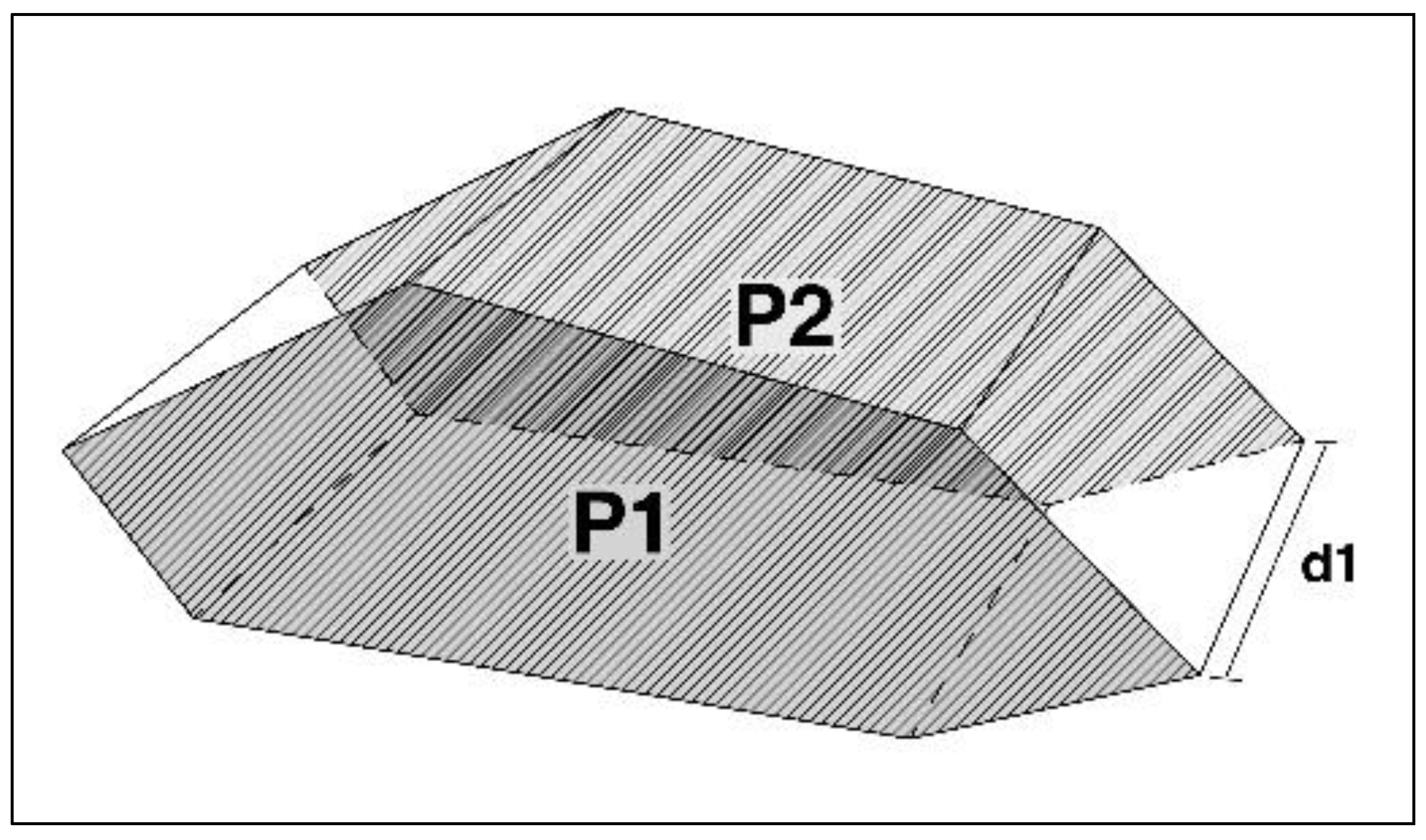
- by cross section;
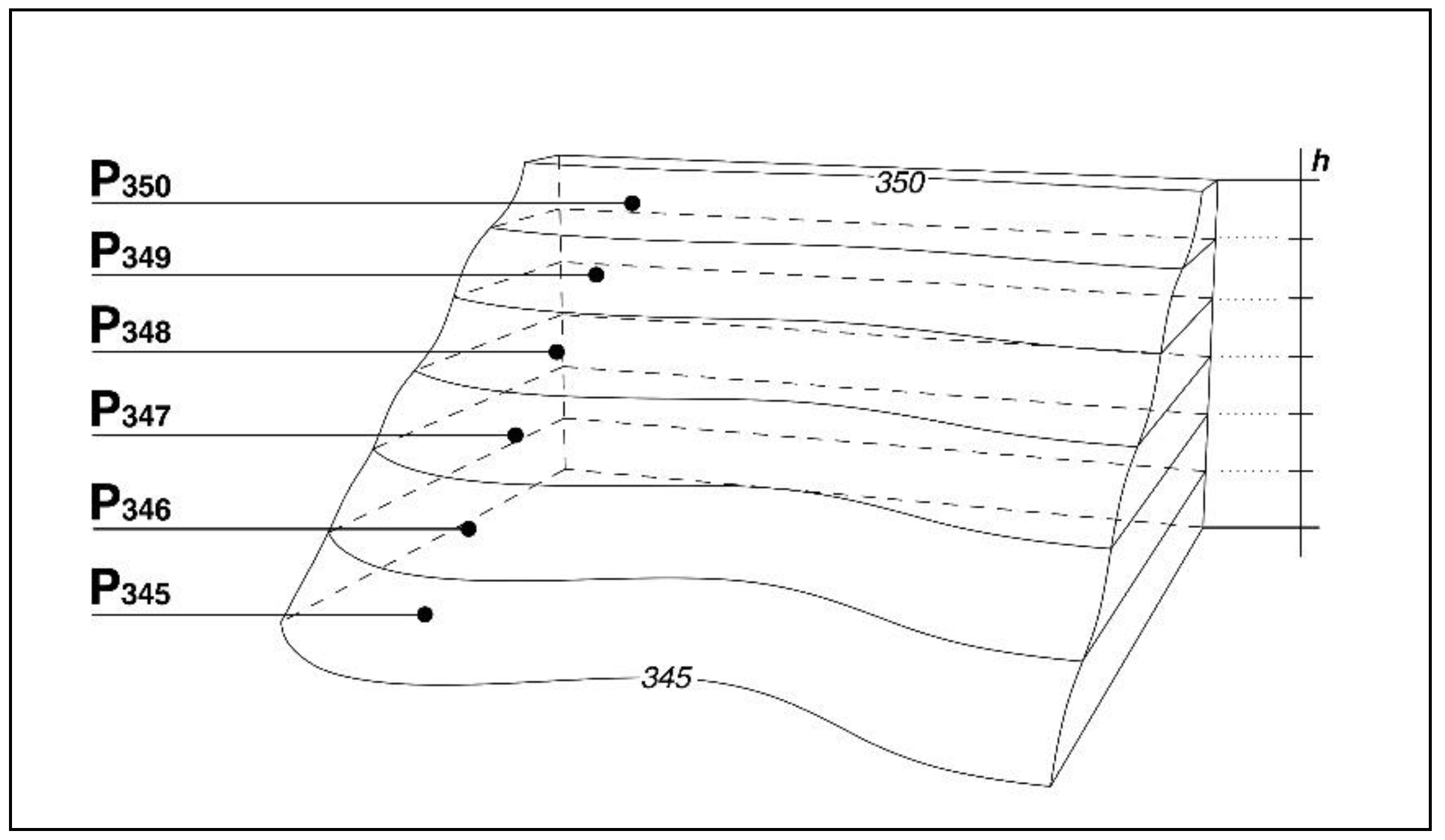
- by horizontal section;
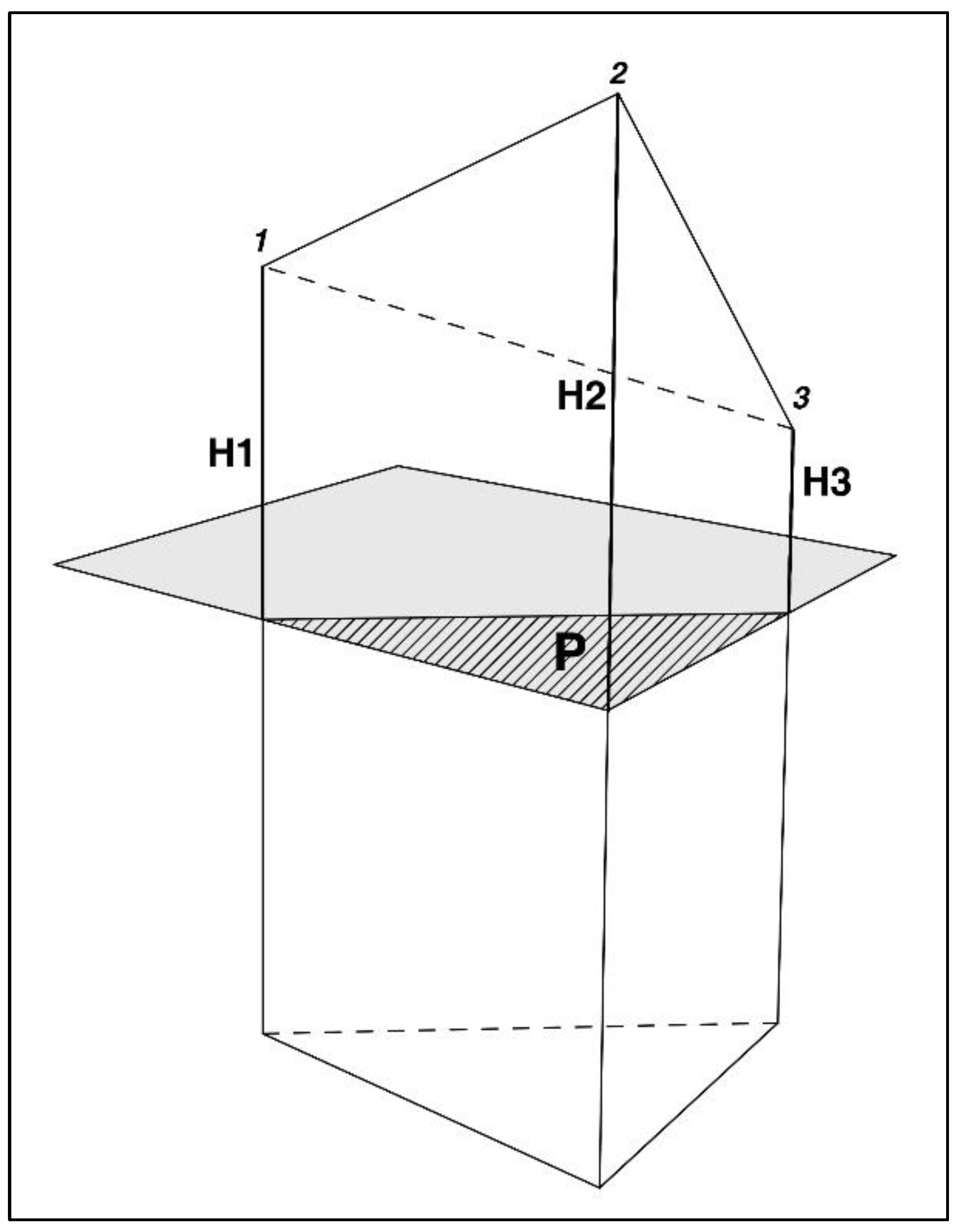
- by prisms between two surfaces;
2.2.1. The Influence of the Surveying Method
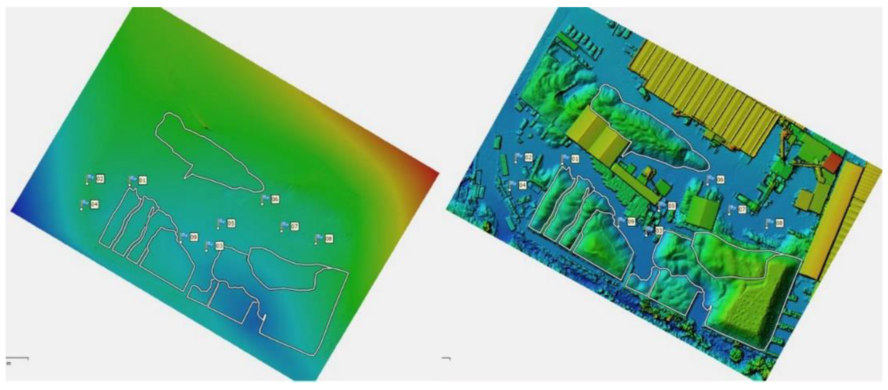
2.2.2. Elevation Models
- vector-based data modelling (Triangulated irregular network - TIN);
- raster-based data modelling (Raster Digital Elevation Modelling - DEM).
2.2.3. The Definition of the Reference Base
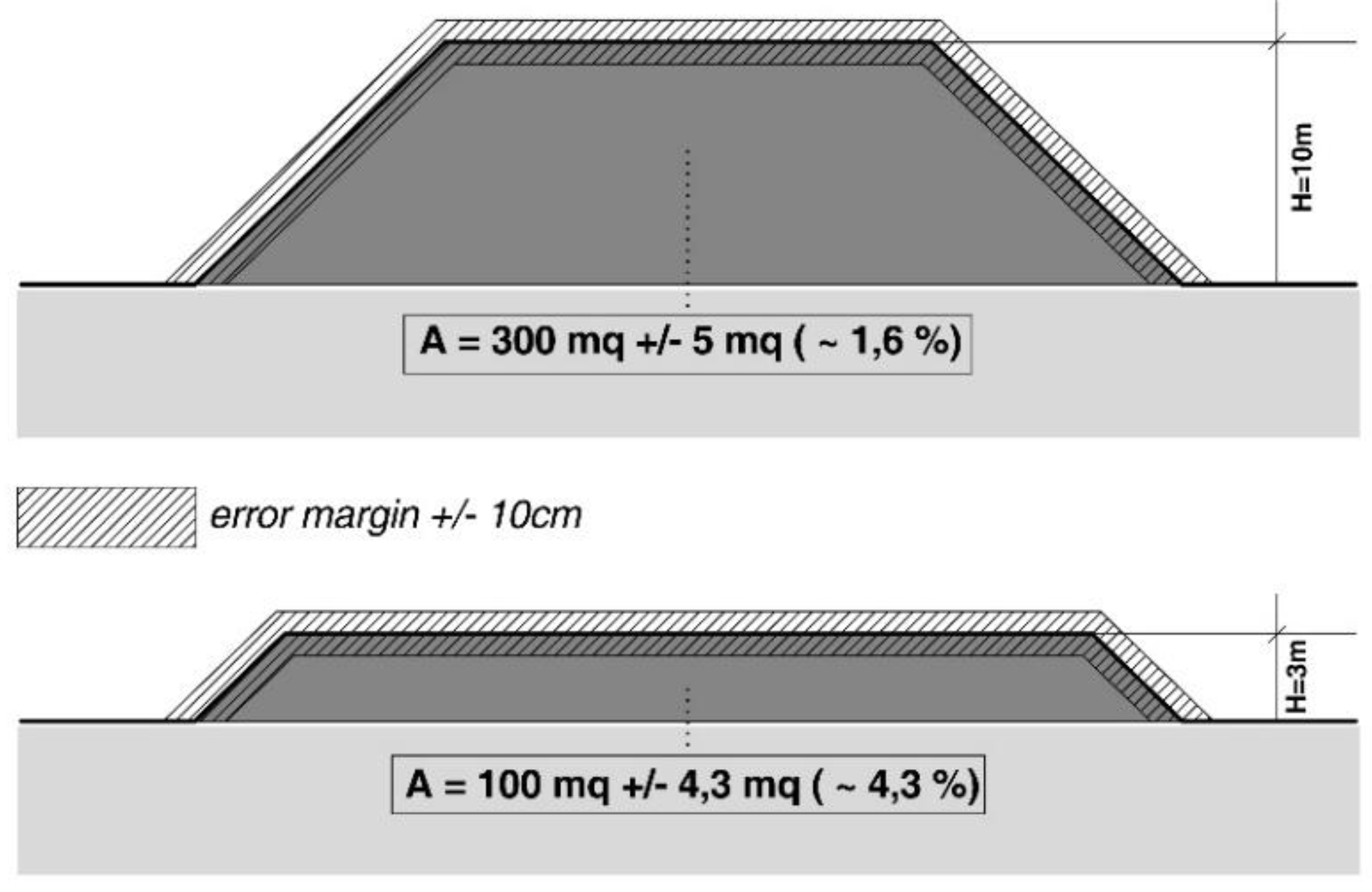
2.2.4. The Influence of the Shapes and Size
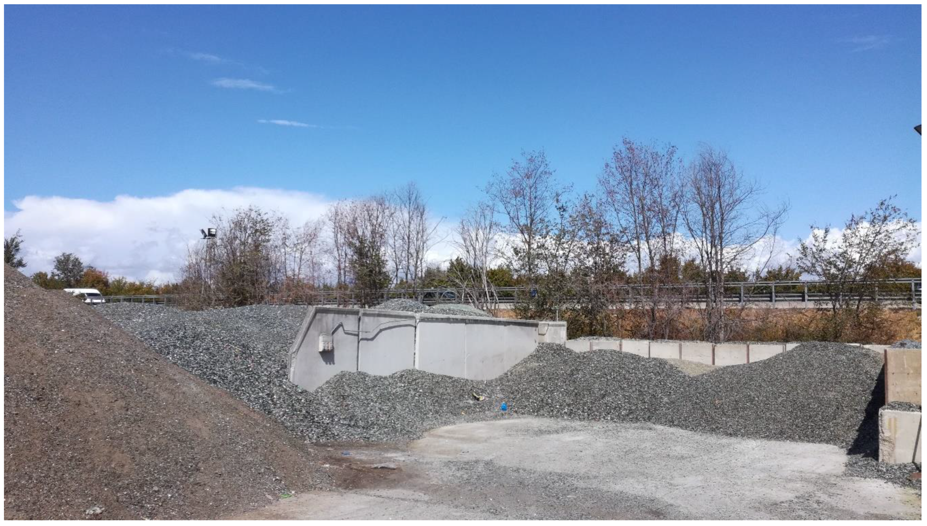
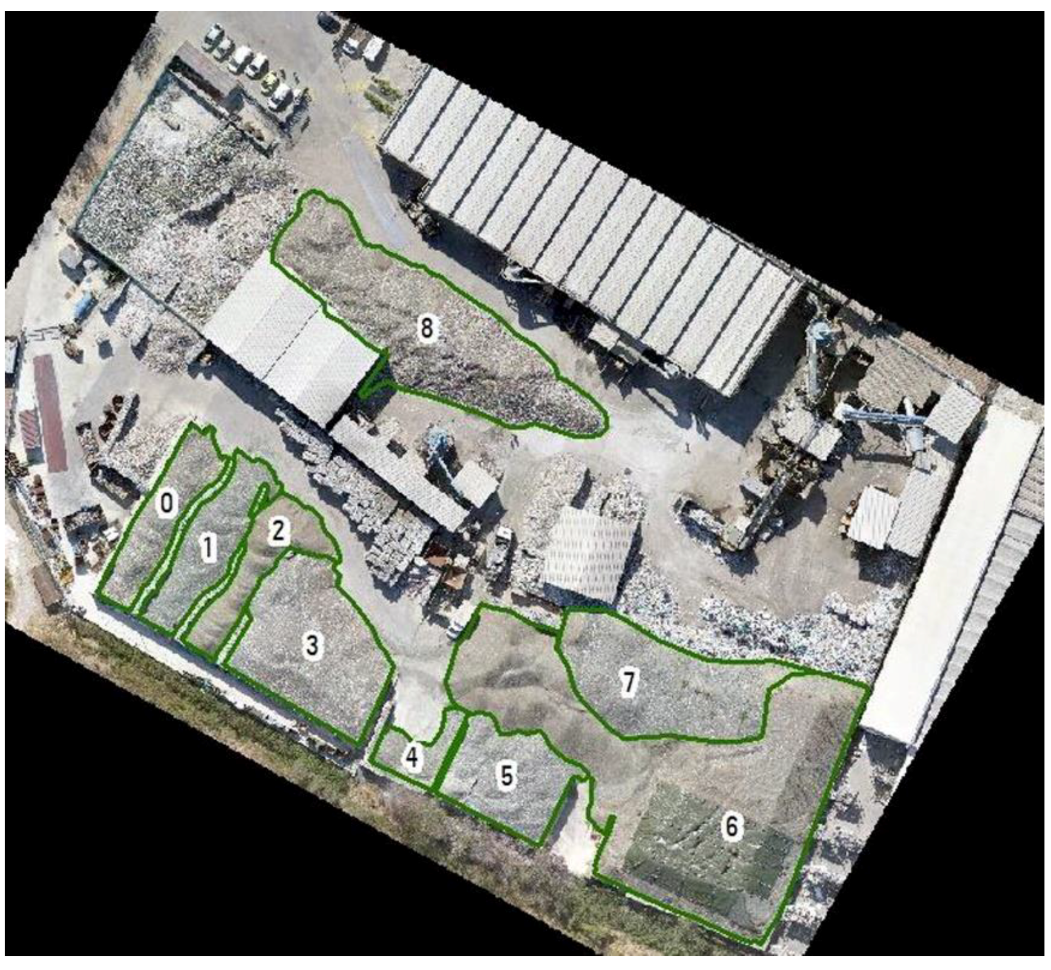
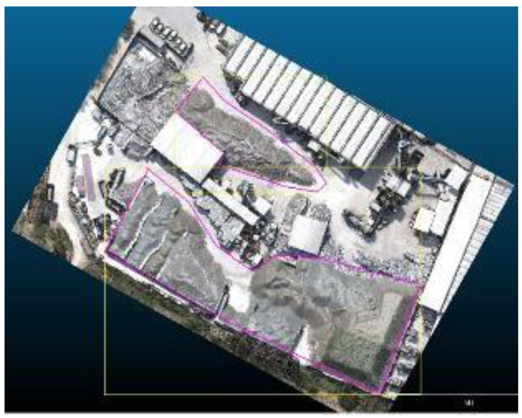
3. Application Experience in a Stockpile Area of Recyclable Waste
3.1. Foreword
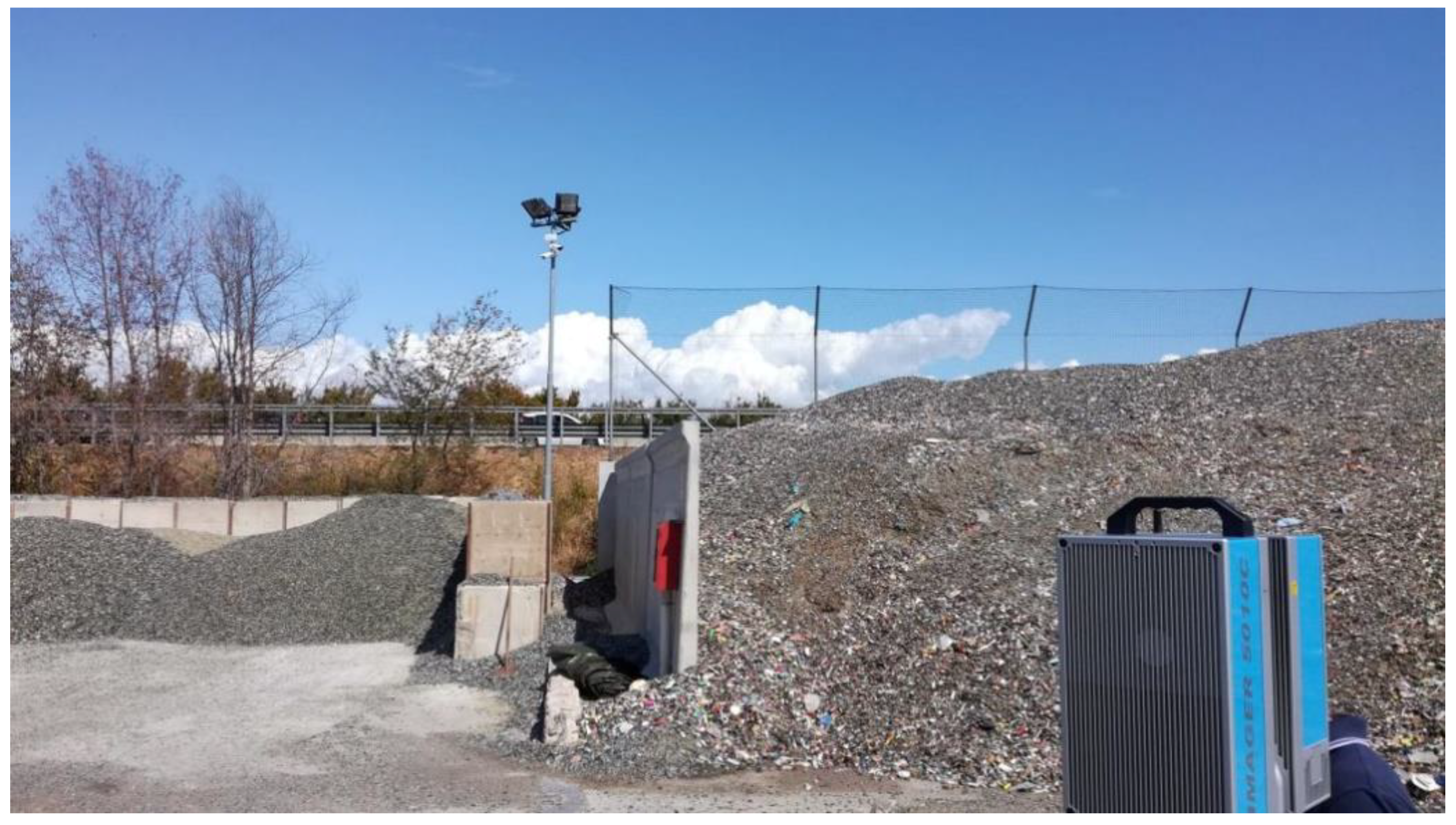
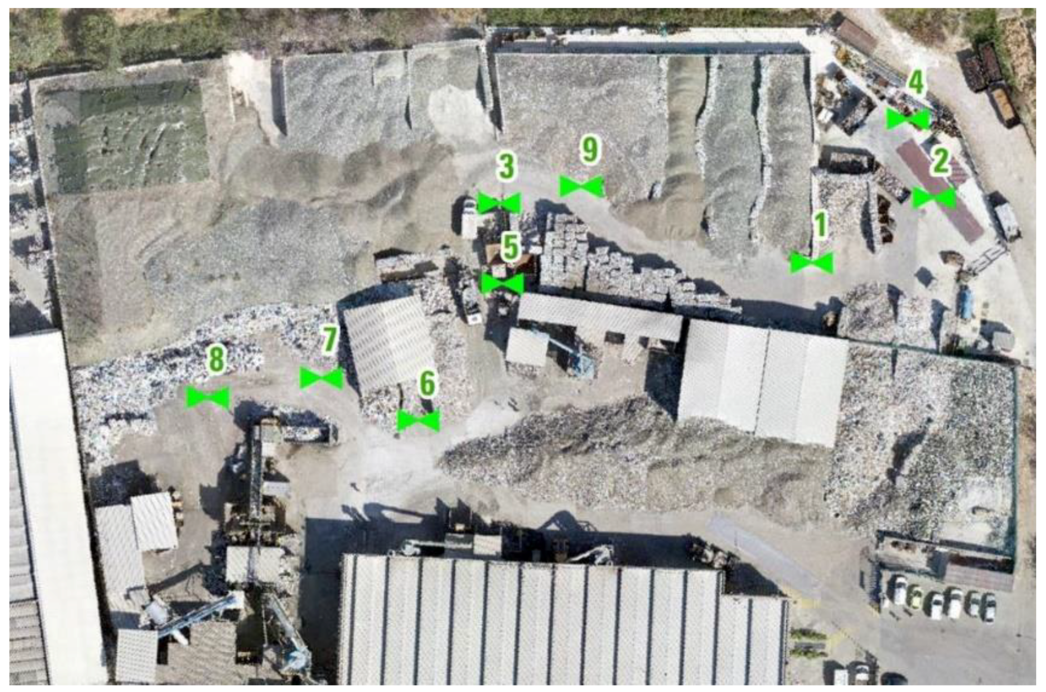
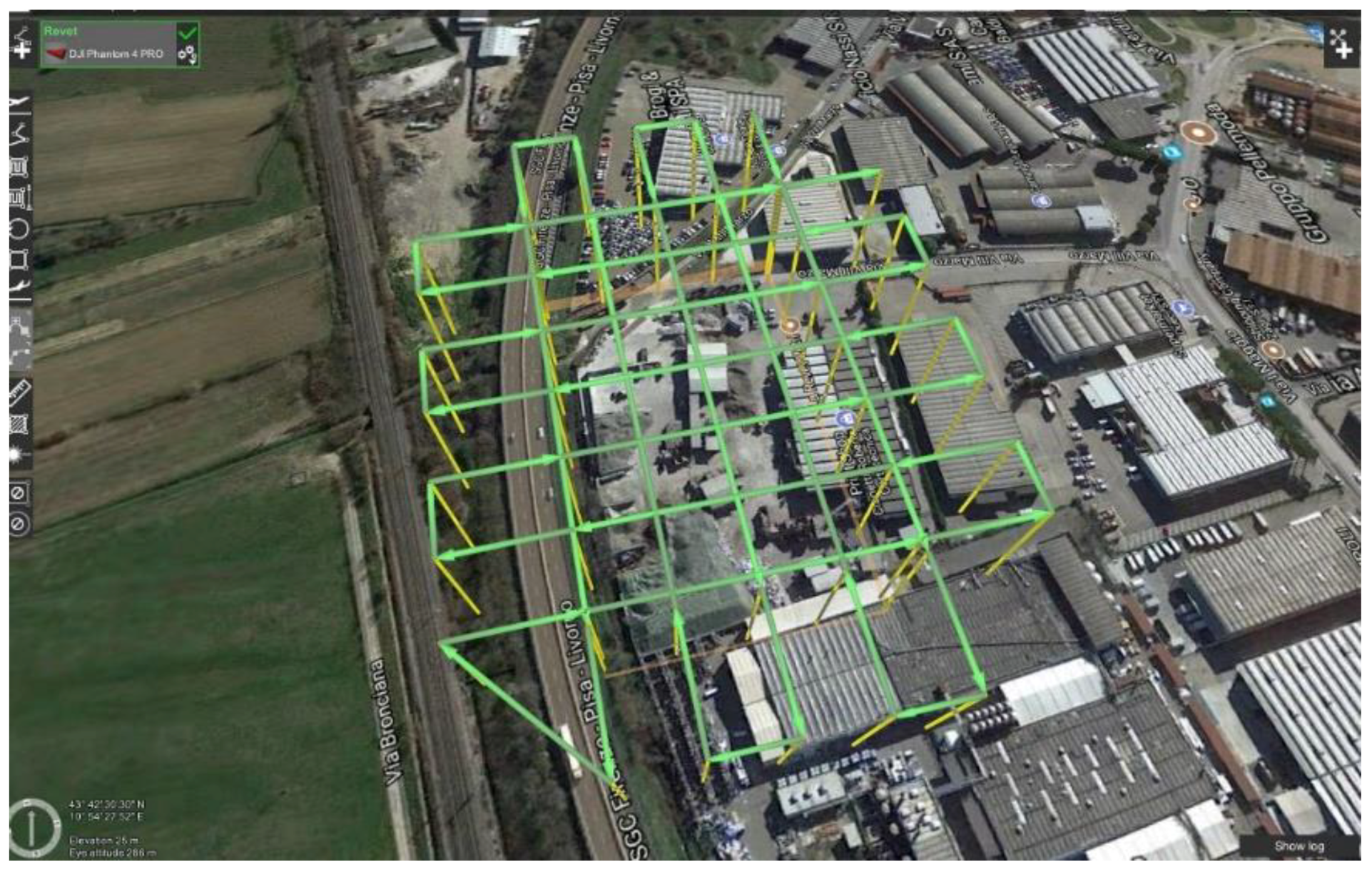
3.2. The Survey
3.3. Processing
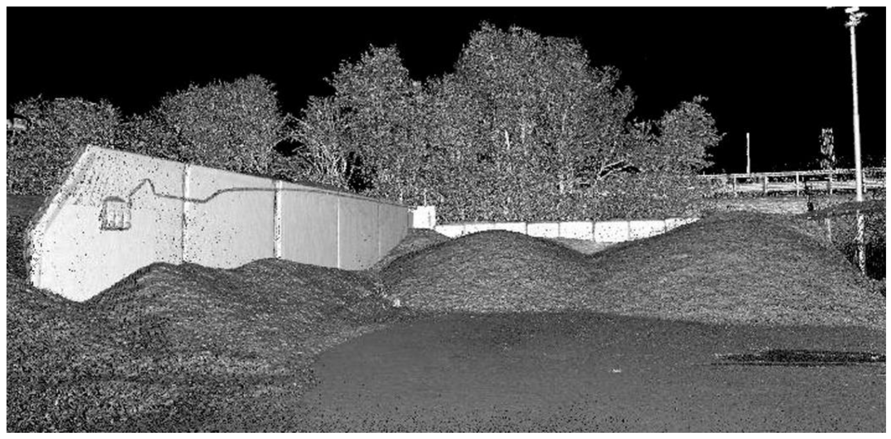
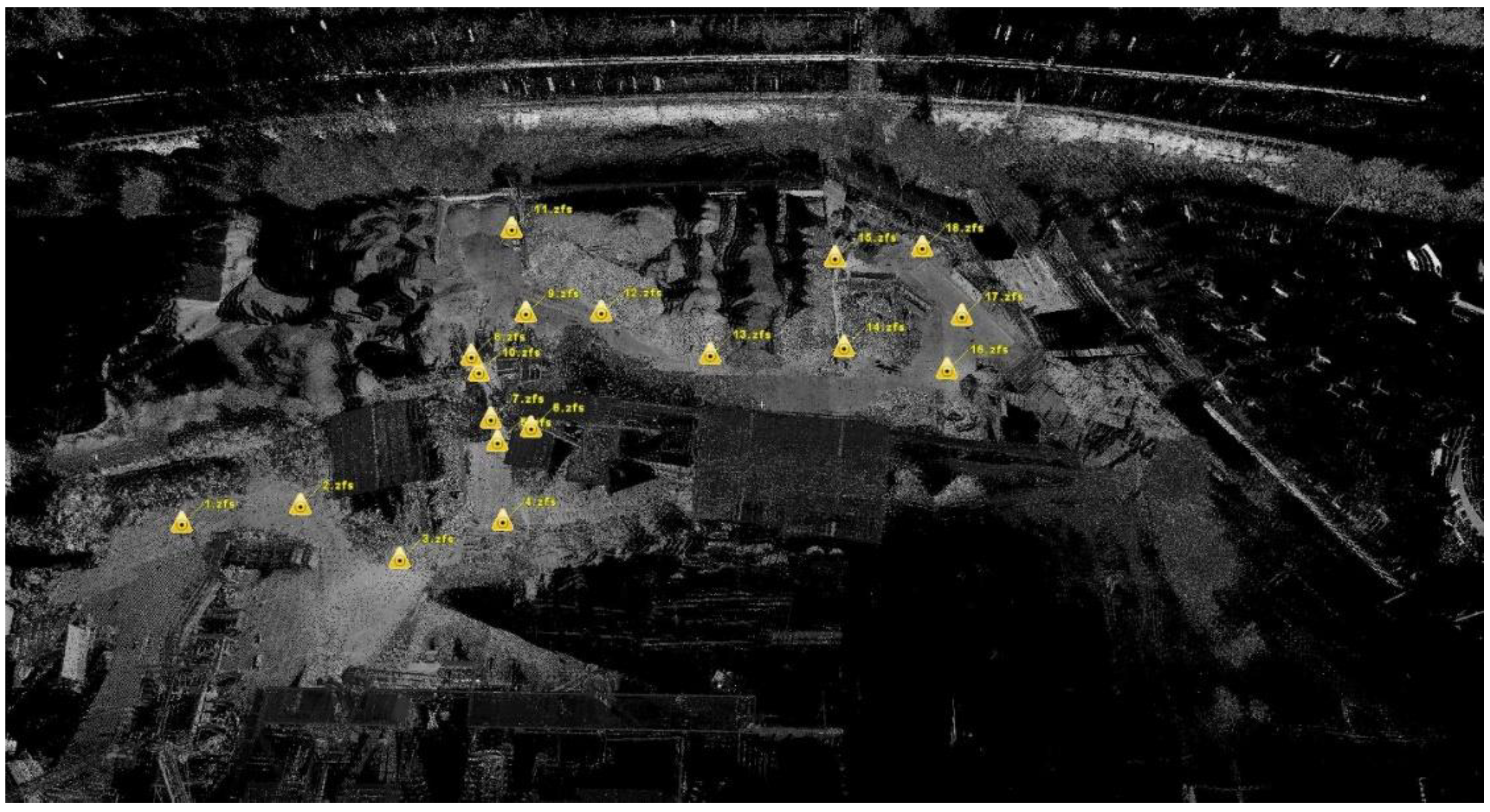
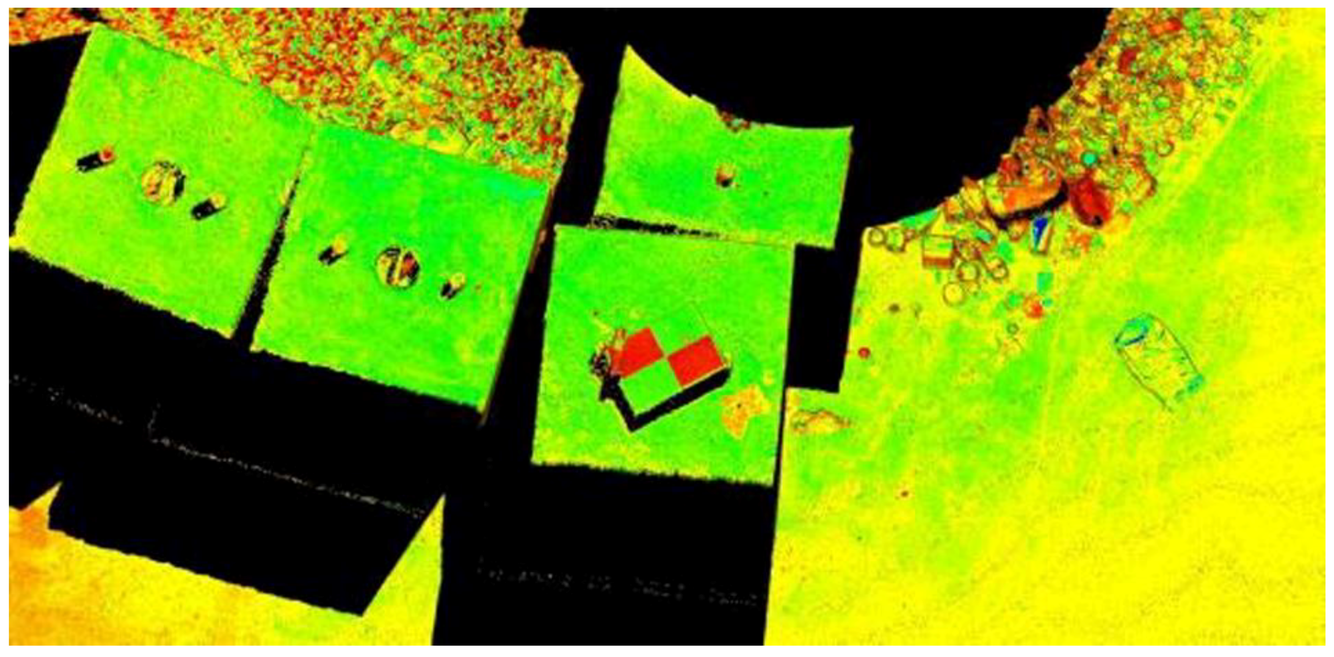
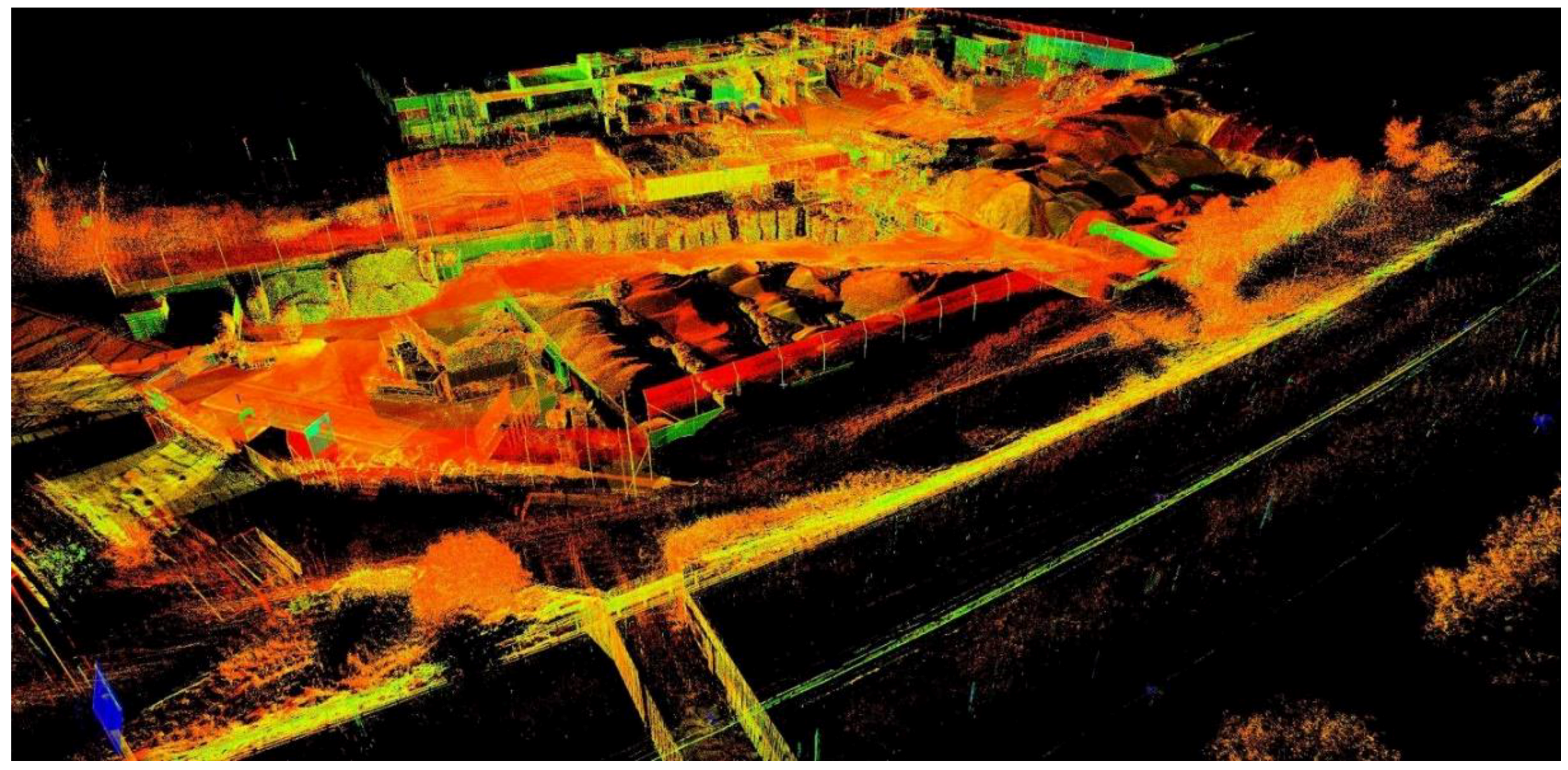
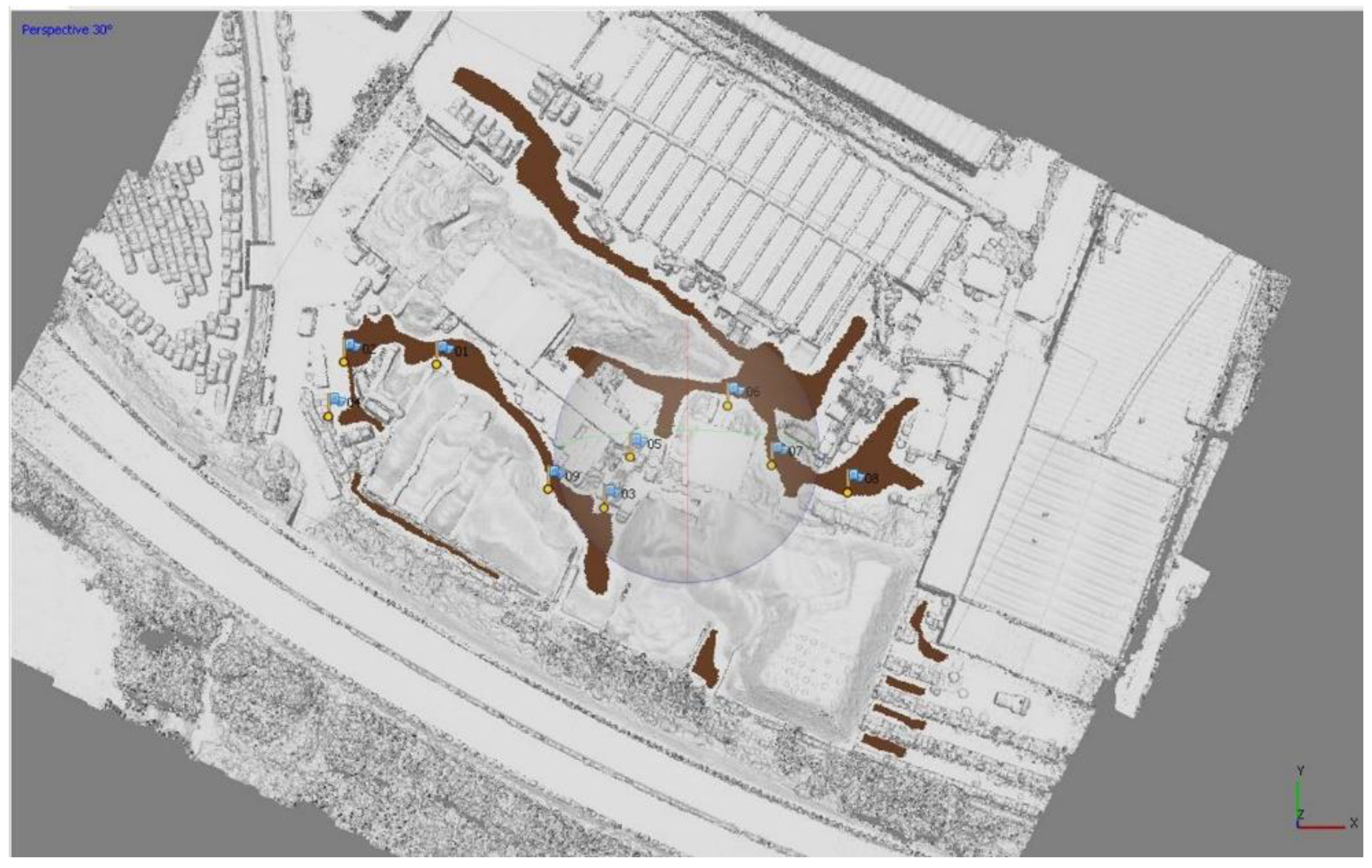
3.3.1. Laser Scanner Survey
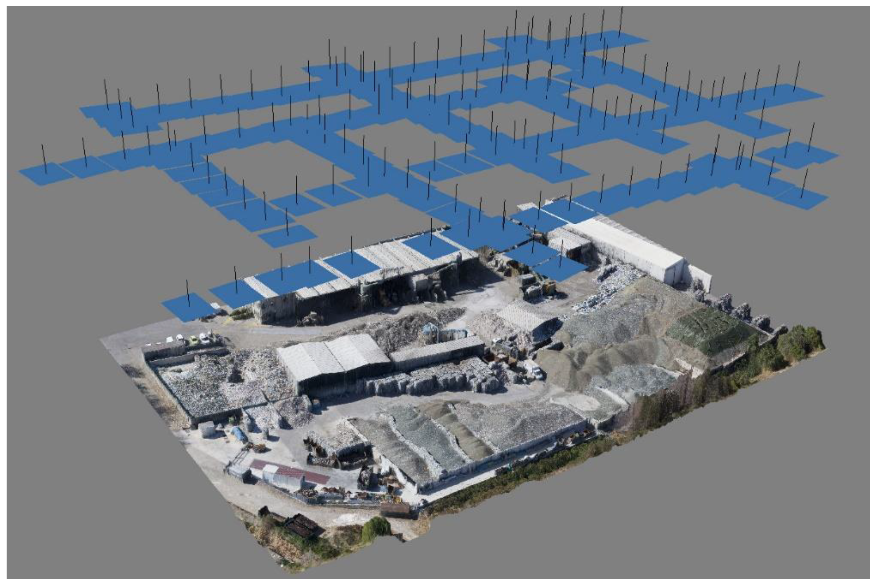
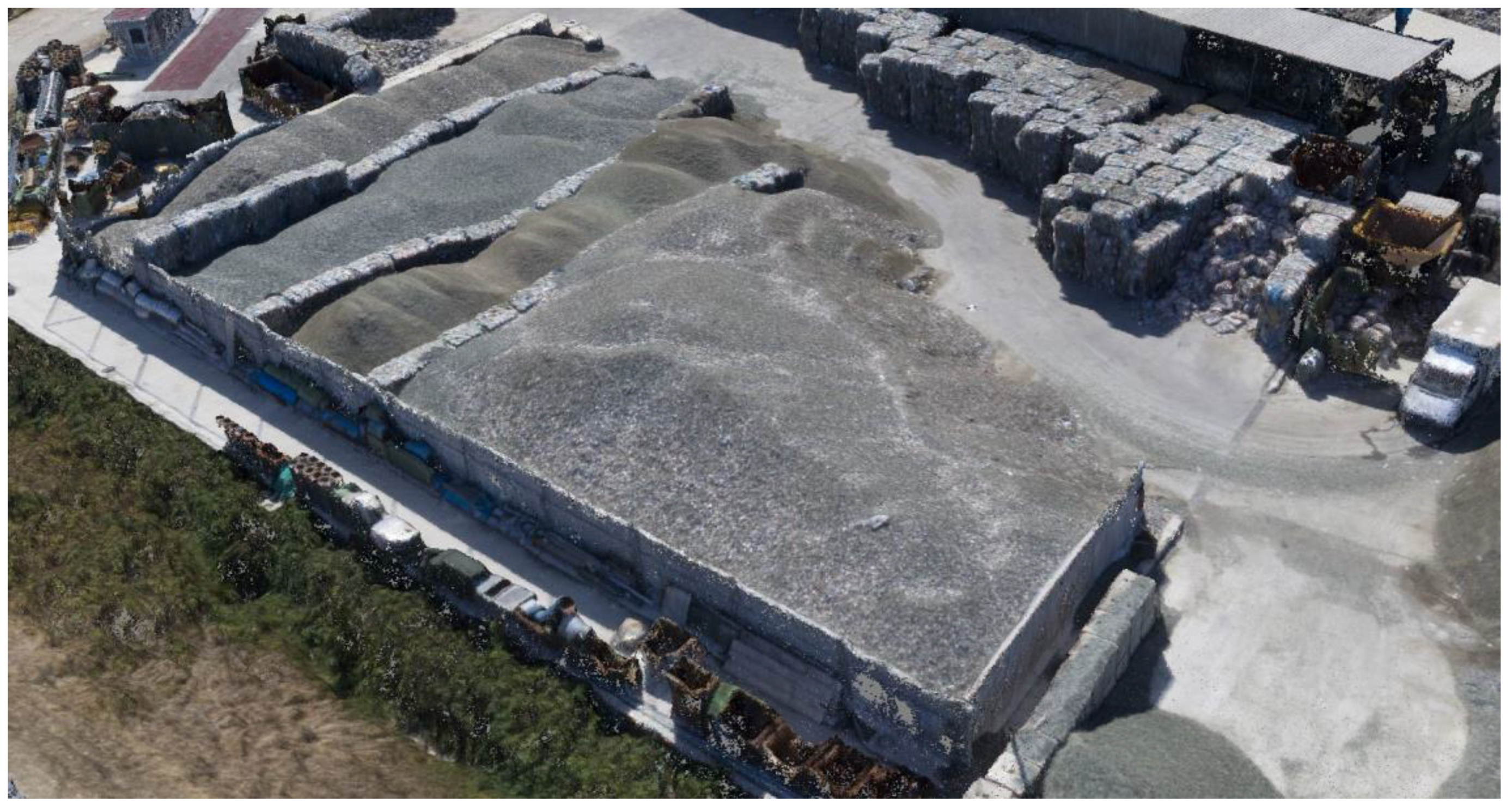
3.3.2. Photogrammetric Survey
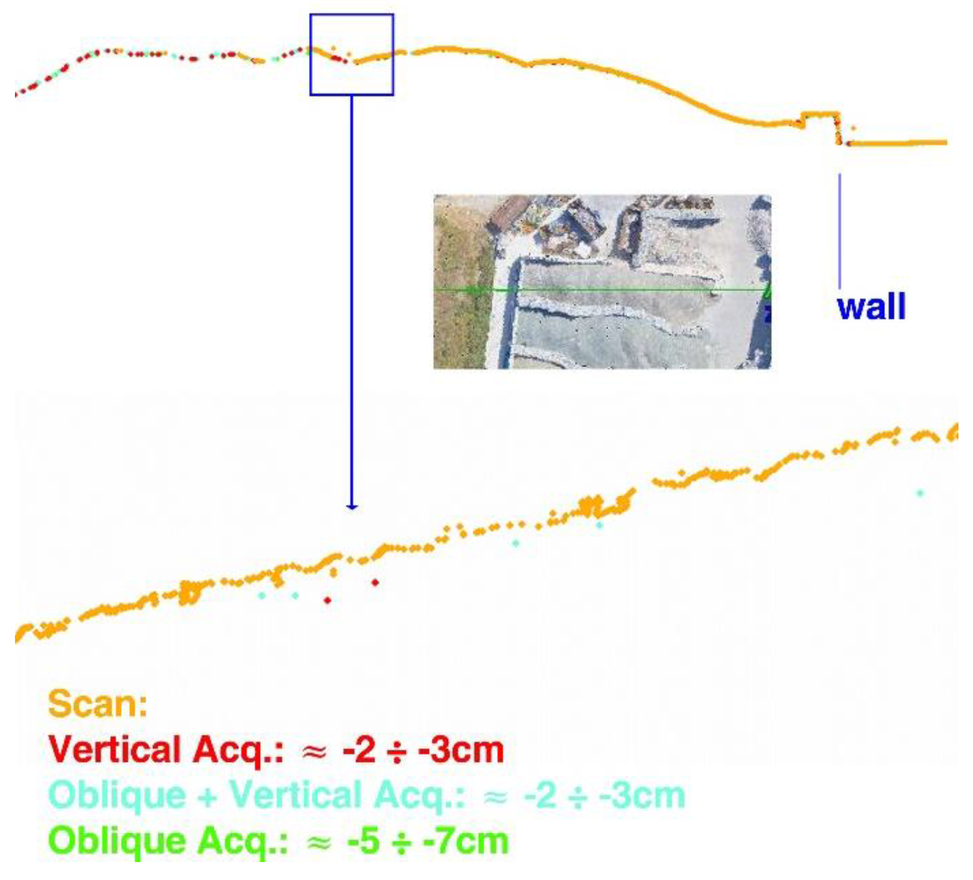
- Vertical camera images only;
- Oblique camera images only;
- Vertical + oblique camera images.
3.4. Volume Measurement
- Agisoft Photoscan;
- Esri ArcGIS [37].
3.4.1. Volume Measurement Procedure with Photoscan
- as an inclined flat surface and interpolated by the vertices of the delimitation of the stockpile (best fit plane);
- as a horizontal flat surface with a medium height determined by the heights of the vertices of the delimitation of the stockpile (mean level plane);
- as a horizontal flat surface at a reference height defined by the user (custom level plane).
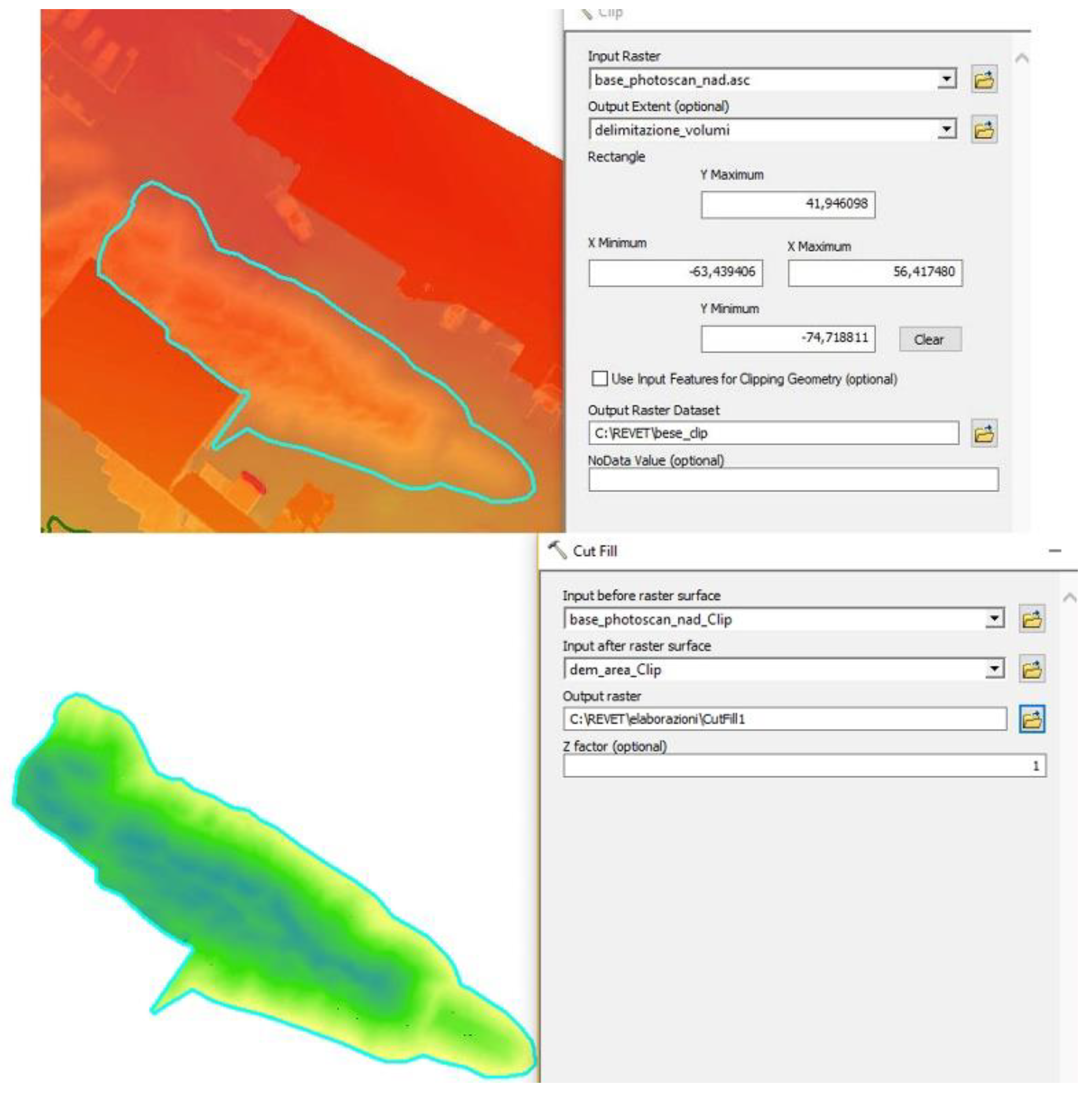
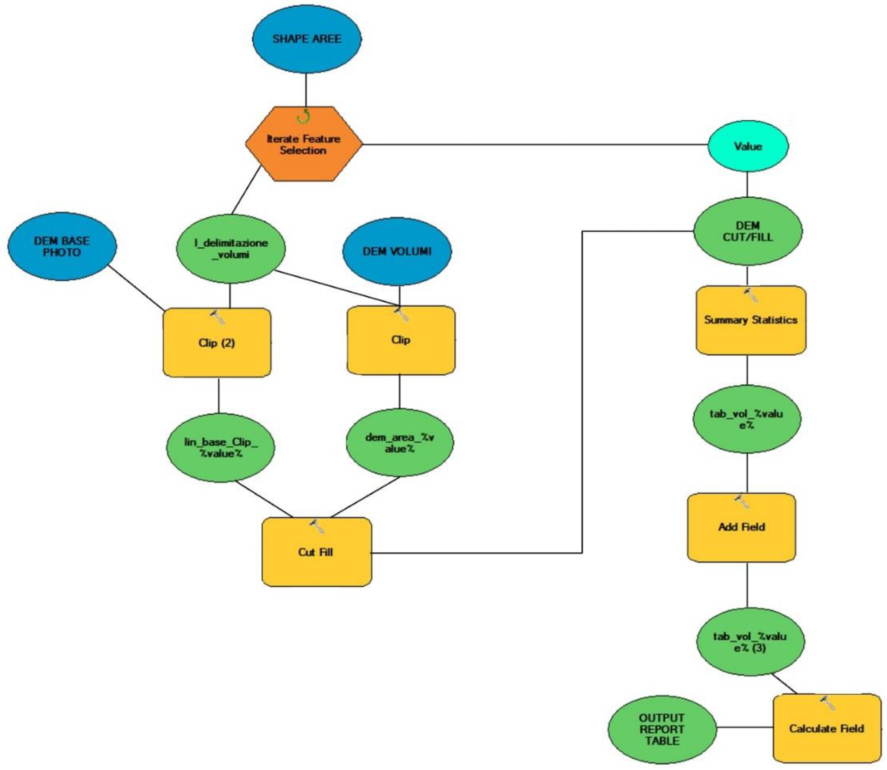
3.4.2. Volume Measurement Procedure with ArcGIS
- the boundaries, contained in a single shapefile with nine area geometry records;
- the DEM of all the surfaces;
- the DEM of the reference base.
4. Results
Volume Assessment
5. Discussion
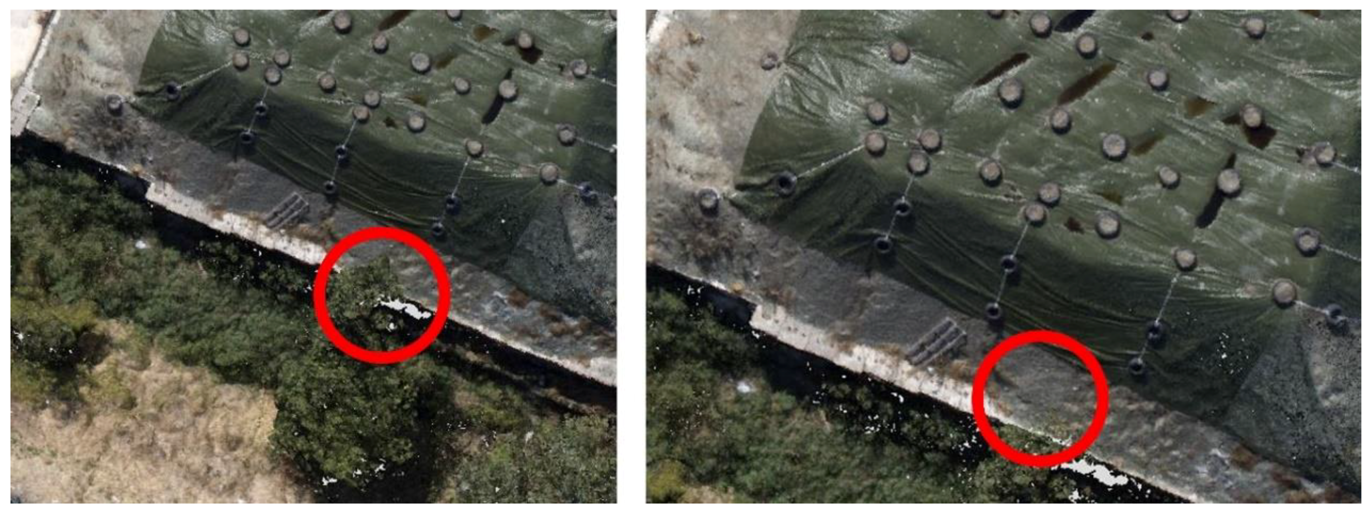
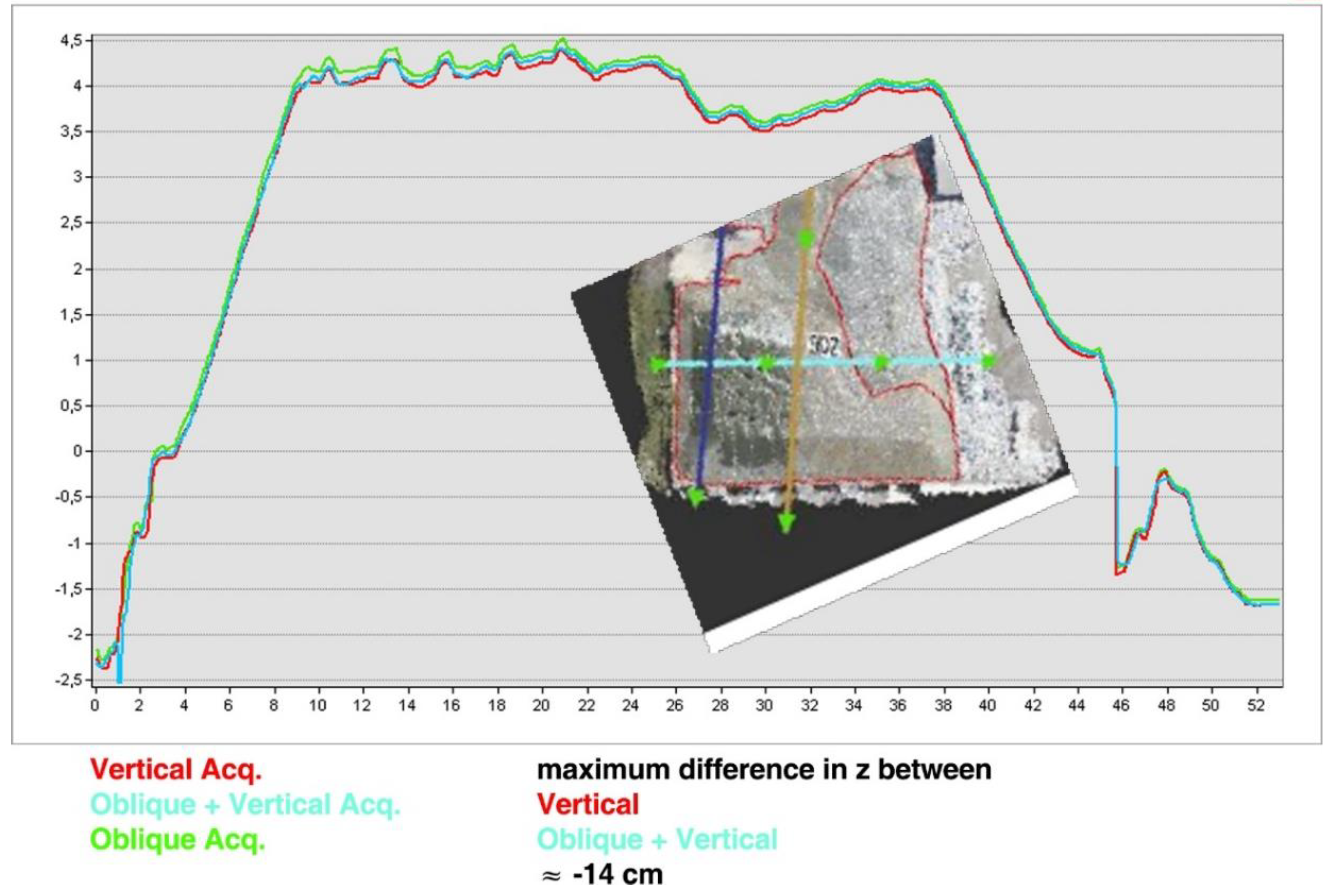
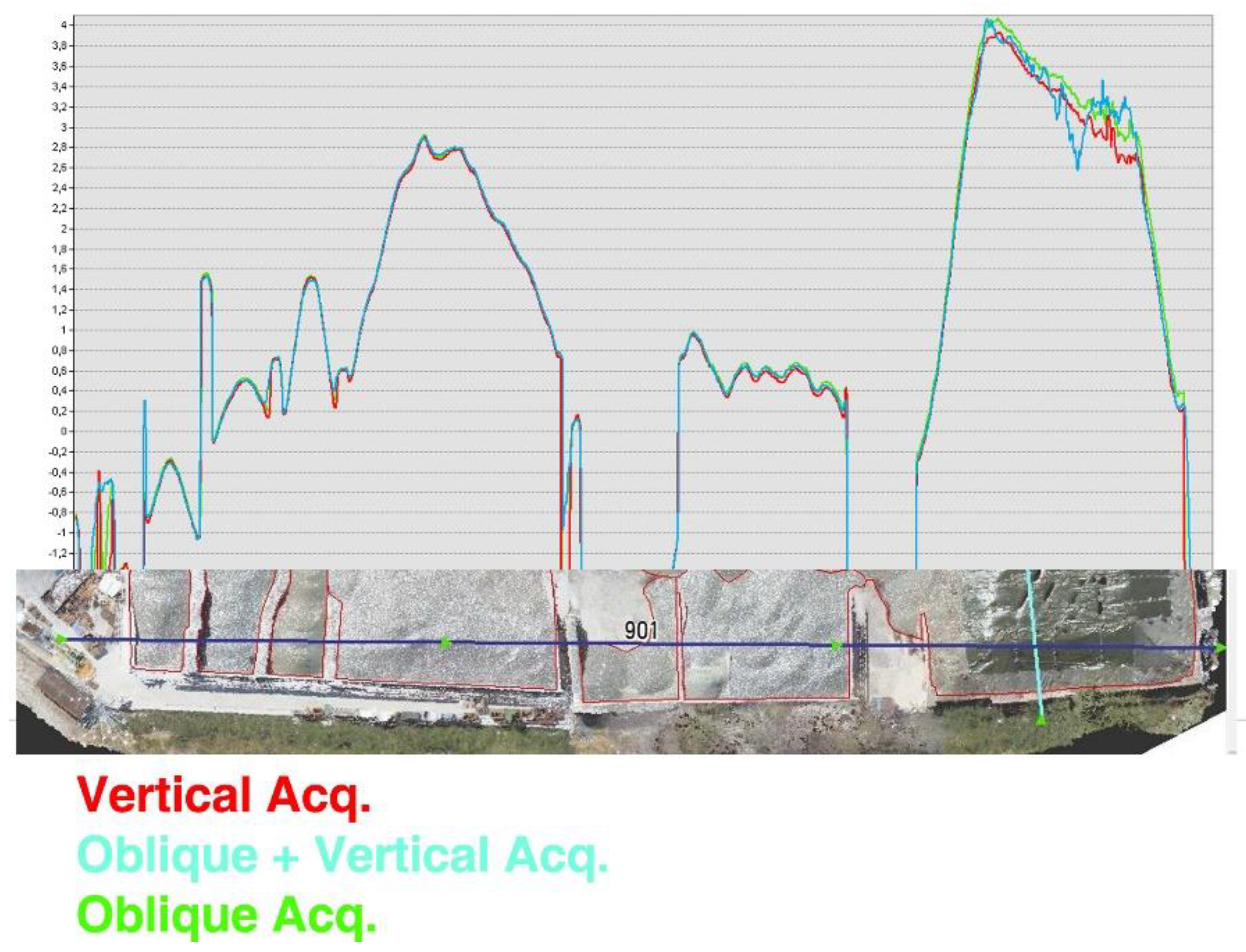
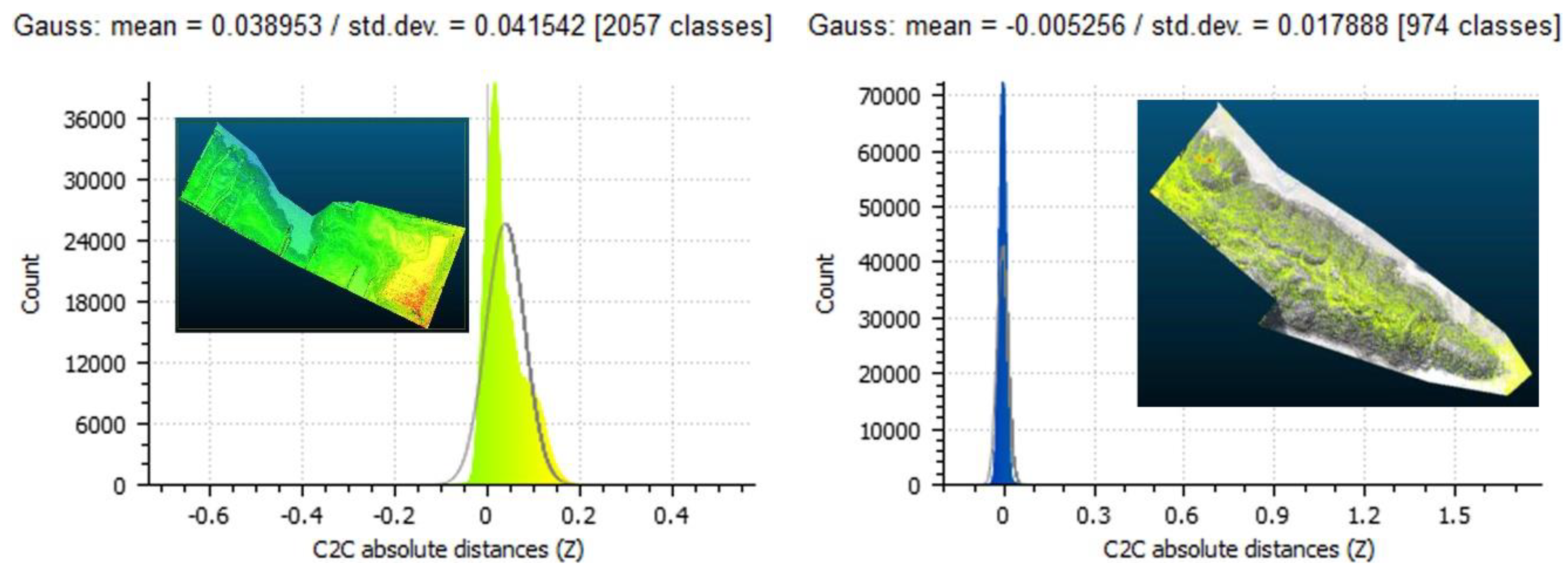
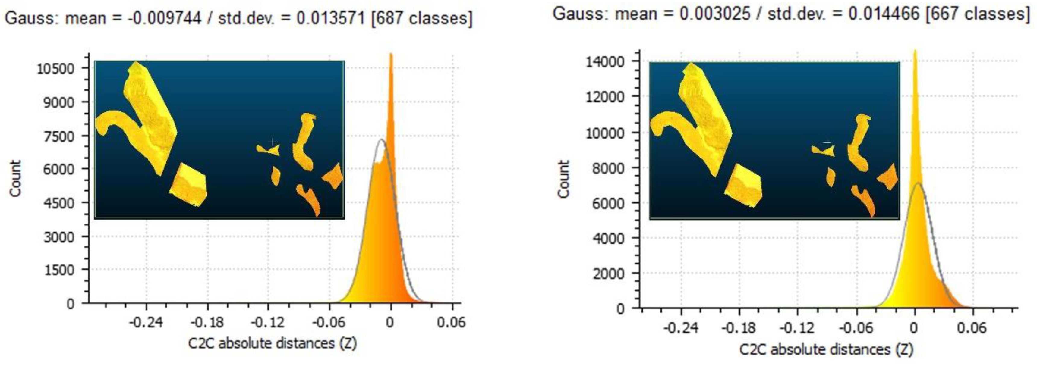
5.1. Comparison Among the Surface Models
5.2. Estimation of the Errors in the Volume Computation
5.3. Evaluation of the Timing
6. Conclusions
Author Contributions
Funding
Acknowledgments
Conflicts of Interest
References
- Randoph Thomas, H.; Riley, D.R.; Messner, J.I. Fundamental Principles of Site Material Management. J. Constr. Eng. Manag. 2005, 131, 808–815. [Google Scholar] [CrossRef]
- De Goede, J.; Muller, B.; Campbell, Q.P.; le Roux, M.; Espag de Klerk, C.B. The effect of particle size on the rate and depth of moisture evaporation from coal stockpiles. J. S. Afr. Inst. Min. Metall. 2016, 116, 353–355. [Google Scholar] [CrossRef] [Green Version]
- Novak, L.; Bizjan, B.; Pražnikar, J.; Horvat, B.; Orbanić, A.; Širok, B. Numerical modeling of dust lifting from a complex-geometry industrial stockpile. Stroj. Vestn./J. Mech. Eng. 2015, 61, 11. [Google Scholar] [CrossRef]
- Connell, J. Almond harvest operations in California—Mantaining nut quality. Acta Hortic. 1994, 373, 241–248. [Google Scholar] [CrossRef]
- Tam, V.W.Y.; Tam, C.M. A review on the viable technology for construction waste recycling. Resour. Conserv. Recycl. 2006, 47, 209–221. [Google Scholar] [CrossRef] [Green Version]
- Tziavou, O.; Pytharouli, S.; Souter, J. Unmanned Aerial Vehicle (UAV) based mapping in engineering geological surveys: Considerations for optimum results. Eng. Geol. 2018, 232, 12–21. [Google Scholar] [CrossRef] [Green Version]
- Sayab, M.; Aerden, D.; Paananen, M.; Saarela, P. Virtual Structural Analysis of Jokisivu Open Pit Using ‘Structure-from-Motion’ Unmanned Aerial Vehicles (UAV) Photogrammetry: Implications for Structurally-Controlled Gold Deposits in Southwest Finland. Remote Sens. 2018, 10, 1296. [Google Scholar] [CrossRef]
- Cook, K.L. An evaluation of the effectiveness of low-cost UAVs and structure from motion for geomorphic change detection. Geomorphology 2017, 278, 195–208. [Google Scholar] [CrossRef]
- Rauhala, A.; Tuomela, A.; Davids, C.; Rossi, P.M. UAV Remote Sensing Surveillance of a Mine Tailings Impoundment in Sub-Arctic Conditions. Remote Sens. 2017, 9, 1318. [Google Scholar] [CrossRef]
- Siebert, S.; Teizer, J. Mobile 3D mapping for surveying earthwork projects using an Unmanned Aerial Vehicle (UAV) system. Automat. Constr. 2014, 41, 1–14. [Google Scholar] [CrossRef]
- Lato, M.; Diederichs, M.S.; Hutchinson, D.J.; Harrap, R. Optimization of LiDAR scanning and processing for automated structural evaluation of discontinuities in rockmasses. Int. J. Rock Mech. Min. Sci. 2009, 46, 194–199. [Google Scholar] [CrossRef]
- Riquelme, A.; Abellan, A.; Tomás, R.; Jaboyedoff, M. A new approach for semi-automatic rock mass joints recognition from 3D point clouds. Comput. Geosci. 2016, 68, 38–52. [Google Scholar] [CrossRef]
- Colomina, I.; Molina, P. Unmanned aerial systems for photogrammetry and remote sensing: A review. ISPRS J. Photogramm. Remote Sens. 2014, 92, 79–97. [Google Scholar] [CrossRef] [Green Version]
- Snavely, N.; Seitz, S.M.; Szeliski, R. Modeling the world from internet photo collections. Int. J. Comput. Vis. 2008, 80, 189–210. [Google Scholar] [CrossRef]
- Bianco, S.; Ciocca, G.; Marelli, D. Evaluating the Performance of Structure from Motion Pipelines. J. Imaging 2018, 4, 98. [Google Scholar] [CrossRef]
- Agüera-Vega, F.; Carvajal-Ramírez, F.; Martínez-Carricondo, P. Accuracy of digital surface models and orthophotos derived from unmanned aerial vehicle photogrammetry. J. Surv. Eng. ASCE 2017, 143, 04016025. [Google Scholar] [CrossRef]
- Arango, C.; Morales, C.A. Comparison between multicopter UAV and Total Station for estimating stockpile volumes. Int. Arch. Photogramm. Remote Sens. Spat. Inf. Sci. 2015, XL-1/W4, 131–135. [Google Scholar] [CrossRef]
- Abbaszadeh, S.; Rastiveisa, H. A Comparison of Close-Range Photogrammetry Using a Non-Professional Camera with Field Surveying for Volume Estimation. Int. Arch. Photogramm. Remote Sens. Spat. Inf. Sci. 2017, XLII-4/W4, 1–4. [Google Scholar] [CrossRef]
- Boscolo Bozza, E.; Di Pietra, V.; Lingua, A.M.; Musci, M.A.; Noardo, F. Fotogrammetria e strumenti GIS per il monitoraggio dei volumi in discarica. In Proceedings of the Atti 21 Conferenza Nazionale ASITA, Salerno, Italy, 21–23 November 2017; pp. 161–164, ISBN 978-88-941232-8-9. Available online: http://atti.asita.it/ASITA2017/Pdf/170.pdf (accessed on 20 December 2018).
- Yakar, M.; Yilmaz, H.M. Using in volume computing of digital close range photogrammetry. Int. Arch. Photogramm. Remote Sens. Spat. Inf. Sci. 2008, XXXVII/W3b, 119–124. Available online: https://www.isprs.org/proceedings/XXXVII/congress/3b_pdf/22.pdf (accessed on 20 December 2018).
- Wang, X.; Al-Shabbani, Z.; Sturgill, R.; Kirk, A.; Dadi, G.B. Estimating Earthwork Volumes through Use of Unmanned Aerial Systems. Transp. Res. Rec. 2017, 2630, 1–8. [Google Scholar] [CrossRef]
- Miljković, S.; Kuburić, M.; Ogrizović, V.; Delčev, S.; Gučević, J. Application of Unmanned Aerial Vehicles in determining the cubic contents of material. In Proceedings of the 5th International Conference Contemporary Achievements in Civil Engineering, Subotica, Serbia, 21 April 2017; Bešević, M.T., Ed.; Birografika Distribucija: Subotica, Serbia, 2017; pp. 913–919. [Google Scholar] [CrossRef]
- Labant, S.; Staňková, H.; Weiss, R. Geodetic determining of stockpile volume of mineral excavated in open pit mine. GeoSci. Eng. 2013, LIX, 30–40. [Google Scholar] [CrossRef]
- Hamzah, H.B.; Said, S.M. Measuring volume of stockpile using Imaging Station. Geoinf. Sci. J. 2011, 11, 15–32. Available online: http://eprints.utm.my/id/eprint/27794/1/HazidaBintiHamzah2011_MeasuringVolumeOfStockpileUsing.pdf (accessed on 20 December 2018).
- Zhu, J.; Yang, J.; Fan, J.; Ai, D.; Jang, Y.; Song, H.; Wang, Y. Accurate measurement of granary stockpile volume based on fast registration of multi-station scans. Remote Sens. Lett. 2018, 9–6, 569–577. [Google Scholar] [CrossRef]
- Yakar, M.; Yilmaz, H.M.; Mutluoglu, O. Performance of Photogrammetric and Terrestrial Laser Scanning Methods in Volume Computing of Excavation and Filling Areas. Arab. J. Sci. Eng. 2014, 39, 387. [Google Scholar] [CrossRef]
- Park, H.J.; Turner, R.; Rak Lee, D.; One Lee, J. 3D modelling of coal stockpiles using UAV data in an open cut mine environment. In Proceedings of the 16th International Congress for Mine Surveying ISM 2016, Brisbane, Australia, 12–16 September 2016; Jarosz, A., Ed.; Ellipsis Media: Toowoomba, Australia, 2016; pp. 77–79. Available online: https://www.minesurveyors.com.au/files/ISM2016/Proceedings/Section3/3_HJ_Park.pdf (accessed on 20 December 2018).
- Chen, L. Fast and Accurate Volume Measurement—The Reason Why Half of the Largest Mining Companies Use Pix4Dmapper Pix4D White Paper 2016. Available online: https://pix4d.com/drone-mining-stockpile-volume-pix4dmapper/ (accessed on 20 December 2018).
- Kern, F. Precise determination of volume with terrestrial 3D-laser scanner. In Proceedings of the 2nd Symposium on Geodesy for Geotechnical and Structural Engineering, Berlin, Germany, 21–24 May 2002; Kahmen, H., Niemeier, W., Retscher, G., Eds.; Vienna University of Technology: Vienna, Austria, 2002; pp. 531–534, ISBN 395014921X. Available online: http://www.xdesy.de/paper/berlin-eng.pdf (accessed on 20 December 2018).
- Draeyer, B.; Strecha, C. White Paper: How Accurate Are UAV Surveying Methods? Pix4D White Paper 2016. Available online: https://pix4d.com/wp-content/uploads/2016/11/Pix4D-White-paper_How-accurate-are-UAV-surveying-methods.pdf (accessed on 20 December 2018).
- Rossi, P.; Mancini, F.; Dubbini, M.; Mazzone, F.; Capra, A. Combining nadir and oblique UAV imagery to reconstruct quarry topography: Methodology and feasibility analysis. Eur. J. Remote Sens. 2017, 50, 211–221. [Google Scholar] [CrossRef]
- Zoller+Fröhlich 5010c. Available online: https://www.zf-laser.com/fileadmin/editor/Datenblaetter/Z_F_IMAGER_5010C_Datasheet_E.pdf (accessed on 20 December 2018).
- DJI Phantom4Pro. Available online: https://www.dji.com/de/phantom-4-pro/info (accessed on 20 December 2018).
- SPH Engineering UgCS vers.2.12. Available online: https://www.ugcs.com/ (accessed on 20 December 2018).
- Leica Geosystems Cyclone vers. 9.1.4. Available online: https://leica-geosystems.com/ (accessed on 20 December 2018).
- Agisoft Photoscan vers.1.4.2. Available online: https://www.agisoft.com (accessed on 20 December 2018).
- Esri ArcGIS vers. 10.6. Available online: https://www.esri.com/ (accessed on 20 December 2018).
- Cryderman, C.; Mah, S.B.; Shufletoski, A. Evaluation of UAV photogrammetric accuracy for mapping and earthworks computations. Geomatica 2014, 68, 309–317. [Google Scholar] [CrossRef]
- Raeva, P.L.; Filipova, S.L.; Filipov, D.G. Volume computation of a stockpile—A study case comparing GPS and UAV measurements in an open pit quarry. Int. Arch. Photogramm. Remote Sens. Spat. Inf. Sci. 2016, XLI-B1, 999–1004. [Google Scholar] [CrossRef]
- CloudCompare vers. 2.9.1 [GPL Software]. Available online: http://www.cloudcompare.org (accessed on 20 December 2018).
- Lague, D.; Brodu, N.; Leroux, J. Accurate 3D comparison of complex topography with terrestrial laser scanner: Application to the Rangitikei canyon (N-Z). ISPRS J. Photogramm. Remote. Sens. 2013, 82, 10–26. [Google Scholar] [CrossRef] [Green Version]


| Data | Quantity |
|---|---|
| Number of stations | 18 |
| Nominal resolution | no. 14 SH (3 mm/10 m) no. 4 H (6 mm/10 m) |
| No. of operators | 2 |
| Survey duration | Approx. 3 h |
| Data | Quantity |
|---|---|
| Flight altitude | Approx. 75 m from ground level |
| Forward overlap | 85% |
| Side overlap | 70% |
| Number of images | 139 (vertical camera) 144 (30° oblique camera) |
| Duration | 15 min. per flight |
| Survey duration | Approx. 4 h |
| GCP | X err. (cm) | Y err. (cm) | Z err. (cm) | Tot. err. (cm) | Projections | Image (pix) |
|---|---|---|---|---|---|---|
| 01 | −0.011 | −0.253 | −0.300 | 0.393 | 45 | 0.093 |
| 03 | −0.244 | −0.176 | −0.790 | 0.845 | 52 | 0.155 |
| 04 | −0.121 | 0.163 | 0.121 | 0.236 | 33 | 0.102 |
| 06 | 0.165 | 0.100 | 0.156 | 0.248 | 49 | 0.116 |
| 08 | −0.103 | 0.023 | 0.021 | 0.107 | 45 | 0.100 |
| 09 | 0.321 | 0.146 | 0.812 | 0.885 | 48 | 0.142 |
| Total | 0.189 | 0.160 | 0.485 | 0.545 | 0.122 |
| CP | X err. (cm) | Y err. (cm) | Z err. (cm) | Tot. err. (cm) | Projections | Image (pix) |
|---|---|---|---|---|---|---|
| 02 | 0.110 | 0.794 | 0.657 | 1.036 | 36 | 0.106 |
| 05 | 0.843 | −0.726 | −2.278 | 2.535 | 48 | 0.140 |
| 07 | 0.213 | 0.341 | 0.172 | 0.437 | 51 | 0.128 |
| Total | 0.506 | 0.652 | 1.372 | 1.601 | 0.127 |
| A—Vertical Camera only | B—Oblique Camera only | C—Vertical + Oblique Camera | ||||||||||
|---|---|---|---|---|---|---|---|---|---|---|---|---|
| ID | ArcGIS m3 | Photoscan m3 | Diff. m3 | % | ArcGIS m3 | Photoscan m3 | Diff. m3 | % | ArcGIS m3 | Photoscan m3 | Diff. m3 | % |
| 0 | 394.87 | 394.96 | 0.09 | 0.02 | 397.12 | 397.07 | −0.05 | −0.01 | 398.40 | 398.51 | 0.11 | 0.03 |
| 1 | 460.56 | 460.46 | −0.10 | −0.02 | 463.12 | 463.10 | −0.02 | 0.00 | 465.05 | 464.94 | −0.11 | −0.02 |
| 2 | 388.04 | 388.09 | 0.05 | 0.01 | 392.29 | 392.38 | 0.09 | 0.02 | 391.09 | 391.21 | 0.12 | 0.03 |
| 3 | 1247.64 | 1248.10 | 0.46 | 0.04 | 1253.00 | 1253.56 | 0.56 | 0.04 | 1256.03 | 1256.49 | 0.46 | 0.04 |
| 4 | 77.29 | 77.33 | 0.04 | 0.05 | 79.61 | 79.63 | 0.02 | 0.02 | 74.75 | 74.88 | 0.13 | 0.17 |
| 5 | 616.58 | 616.71 | 0.13 | 0.02 | 627.99 | 628.34 | 0.35 | 0.06 | 619.57 | 619.71 | 0.14 | 0.02 |
| 6 | 5512.90 | 5515.72 | 2.82 | 0.05 | 5571.03 | 5573.43 | 2.40 | 0.04 | 5559.63 | 5562.68 | 3.05 | 0.05 |
| 7 | 2049.24 | 2049.14 | −0.10 | 0.00 | 2074.82 | 2074.80 | −0.02 | 0.00 | 2060.83 | 2060.95 | 0.12 | 0.01 |
| 8 | 1519.61 | 1521.93 | 2.32 | 0.15 | 1532.28 | 1533.82 | 1.54 | 0.10 | 1535.67 | 1537.01 | 1.34 | 0.09 |
| A Vertical | B Oblique | C ver. + obl. | B-A | C-A | ||||
|---|---|---|---|---|---|---|---|---|
| ID | Area m2 | Volume m3 | Volume m3 | Volume m3 | Volume m3 | % | Volume m3 | % |
| 0 | 197 | 394.87 | 397.12 | 398.40 | 2.25 | 0.57 | 3.53 | 0.89 |
| 1 | 221 | 460.56 | 463.12 | 465.05 | 2.56 | 0.56 | 4.49 | 0.97 |
| 2 | 185 | 388.04 | 392.29 | 391.09 | 4.24 | 1.09 | 3.05 | 0.79 |
| 3 | 457 | 1247.64 | 1253.00 | 1256.03 | 5.36 | 0.43 | 8.39 | 0.67 |
| 4 | 86 | 77.29 | 79.61 | 74.75 | 2.32 | 3.00 | −2.54 | −3.29 |
| 5 | 267 | 616.58 | 627.99 | 619.57 | 11.40 | 1.85 | 2.99 | 0.48 |
| 6 | 1401 | 5512.90 | 5571.03 | 5559.63 | 58.13 | 1.05 | 46.73 | 0.85 |
| 7 | 461 | 2049.24 | 2074.82 | 2060.83 | 25.58 | 1.25 | 11.59 | 0.57 |
| 8 | 753 | 1519.61 | 1532.28 | 1535.67 | 12.67 | 0.83 | 16.05 | 1.06 |
| S/V Ratio | ||||||||
|---|---|---|---|---|---|---|---|---|
| 0 | 1 | 2 | 3 | 4 | 5 | 6 | 7 | 8 |
| 0.49 | 0.48 | 0.47 | 0.36 | 1.15 | 0.43 | 0.25 | 0.22 | 0.49 |
| V (m3) | S (m2) | |||
|---|---|---|---|---|
| 0 | 398.40 | 197 | 4.04 | 1.01 |
| 1 | 465.05 | 221 | 4.53 | 0.97 |
| 2 | 391.09 | 185 | 3.79 | 0.97 |
| 3 | 1256.03 | 457 | 9.37 | 0.75 |
| 4 | 74.75 | 86 | 1.76 | 2.36 |
| 5 | 619.57 | 267 | 5.47 | 0.88 |
| 6 | 5559.63 | 1401 | 28.72 | 0.52 |
| 7 | 2060.83 | 461 | 9.45 | 0.46 |
| 8 | 1535.67 | 753 | 15.44 | 1.01 |
| Work Phase | Times |
|---|---|
| UAV photogrammetric survey, including the preparation and control phases | 2 h (one shoot) 3 h (two shoots) |
| Pre-processing, alignment, GCPs insertion and collimation, optimisation | 5 h (approx. 3 for the computation) |
| Dense cloud processing | From 4 to 24 h (depending on the hardware) |
| Editing of dense cloud, creation of mesh + texture, creation of DEM | 1 h |
| Acquisition and exporting delimitation of volumes | 1 h |
| Ground classification and creation of DEM base | 1 h |
| Photoscan: volume computation | 30 min |
| ArcGIS: data importation and volume computation (builder model) | 30 min |
| TOTAL SURVEY AND COMPUTATION PHASE (with the best hardware configuration) | 3 h survey; 5 h interactive processing; 7 h automatic processing. 30 min computation |
© 2019 by the authors. Licensee MDPI, Basel, Switzerland. This article is an open access article distributed under the terms and conditions of the Creative Commons Attribution (CC BY) license (http://creativecommons.org/licenses/by/4.0/).
Share and Cite
Tucci, G.; Gebbia, A.; Conti, A.; Fiorini, L.; Lubello, C. Monitoring and Computation of the Volumes of Stockpiles of Bulk Material by Means of UAV Photogrammetric Surveying. Remote Sens. 2019, 11, 1471. https://0-doi-org.brum.beds.ac.uk/10.3390/rs11121471
Tucci G, Gebbia A, Conti A, Fiorini L, Lubello C. Monitoring and Computation of the Volumes of Stockpiles of Bulk Material by Means of UAV Photogrammetric Surveying. Remote Sensing. 2019; 11(12):1471. https://0-doi-org.brum.beds.ac.uk/10.3390/rs11121471
Chicago/Turabian StyleTucci, Grazia, Antonio Gebbia, Alessandro Conti, Lidia Fiorini, and Claudio Lubello. 2019. "Monitoring and Computation of the Volumes of Stockpiles of Bulk Material by Means of UAV Photogrammetric Surveying" Remote Sensing 11, no. 12: 1471. https://0-doi-org.brum.beds.ac.uk/10.3390/rs11121471